Sage Journals: Discover world-class research

Abstract

When individuals are released from prison, they typically enter a period of post confinement community supervision. While under community supervision, their behaviors are subject to special conditions requiring them to report to supervisors and prohibiting certain behaviors such as drug and alcohol use. Many supervisees are returned to prison because they violate those special conditions, or because they commit minor crimes that would not result in prison were they not being supervised. But others are returned to prison for serious new crimes. We distinguish the two as nuisance behaviors (the former) and pernicious behaviors (the latter). Our research applies competing events survival analysis to distinguish a structural model that accounts for nuisance behaviors from a structural model that accounts for pernicious behaviors. We demonstrate that returning offenders to prison for technical violations and minor crimes may reduce the incidence of major crimes because the occurrence of nuisance behaviors and pernicious behaviors are highly correlated. Our findings support the theory that nuisance behaviors signal the likelihood of pernicious behaviors.

Keywords

competing events survival models bounding copulas criminal recidivism parole supervision

Introduction

Following a release from prison, most formerly incarcerated persons (FIPs) spend a period under post-confinement community supervision (PCCS). During this period, they can have their supervision revoked and be returned to prison for violating conditions of PCCS, or they can commit a new crime serious enough to warrant a new conviction leading to a prison commitment. In prior research of post-release recidivism, most researchers have lumped both types of events together to analyze them as a return to prison. Assuming homogeneity in the offenses that trigger a return to prison fails to distinguish that some crimes (e.g., homicide) are more serious than others (e.g., petty larceny), and it conflates behaviors that would not result in incarceration if a formerly incarcerated person (FIP) were not on PCCS with more serious crimes that would result in incarceration. The failure to distinguish among these behaviors has policy implications. Lumping less serious and more serious crime together may overstate the degree of recidivism involving serious crimes, which can lead to overincarceration. Also, failure to distinguish crime by level of seriousness could lead to underestimating the risk of committing a more serious crime by persons who engage in the less serious behaviors.

In a small subset of studies, researchers have modeled competing events using standard survival analysis where one event censors the second event. But unless the two competing outcomes are statistically independent conditional on covariates, failure functions estimated from standard survival models will be biased and inconsistent. Estimation may lead to misleading policy recommendations. In fact, we show in our illustration the two types of events are correlated, so standard survival analysis techniques are inapplicable.

In this paper, we propose a method that accommodates competing risks when the events are dependent. We analyze recidivism by the type of prison return—a revocation or new conviction commitment—and estimate separate hazards for each of these types. To frame the problem and illustrate estimation, we use New York State data to study recidivism during the period following prison release when FIPs are under community supervision. Some FIPs return to prison for what we label nuisance behaviors: technical violations of community supervision (such as illegal drug use) or minor crimes (such as petty larceny) that would probably not result in incarceration if the FIPs were not under community supervision. Some other FIPS return to prison for what we label pernicious behaviors: serious crimes (such as homicide) that result in new convictions and imposition of new prison terms. The rest complete PCCS successfully. Our use of pernicious and nuisance is just shorthand for distinguishing criminal behavior of different seriousness as judged by public authorities and otherwise not intended to be descriptive.

Using a competing events model, we estimate the processes leading to nuisance recidivism and pernicious recidivism showing they are highly correlated. Finding high correlation suggests that the commission of nuisance behaviors sends a strong signal that a FIP is at high risk of committing pernicious crimes. In turn, this suggests that revocation practices may be functional: They incapacitate offenders for minor crimes and thereby reduce serious crimes.

Our analytical approach is consistent with recommendations by the National Academy of Sciences (2022). The NAS report noted that recidivism is typically defined broadly to include all crimes without distinctions for seriousness, but a better accounting would distinguish offenses by seriousness. In our analyses, nuisance recidivism is much less serious than pernicious recidivism. Treating them as competing events conforms with the NAS recommendation. Although we use the competing risk model to study PCCS outcomes, the technique should have broader application in criminal justice research: Program evaluations might consider reductions in the seriousness of recidivism as a criterion of success. Risk prediction might differentiate risk for less serious and more serious recidivism. Studies of criminal careers might expand beyond simple measures of criminality.

The next section is an overview of PCCS. This is followed by an introduction to competing events modeling and an explanation of our model. Then we describe our data, present empirical findings, and discuss results.

Competing Events: Community Supervision Outcomes

According to the U.S. Bureau of Justice Statistics (Kaeble, 2021), at the end of 2020, an estimated 850,964 adults were under PCCS. The duration of PCCS is determined by some combination of criminal statutes, the judicial sentence, and by an administrative agency such as a parole board. During 2020, about 57% of adults who ended supervision successfully completed their community supervision, and with exceptions such as death, the rest were revoked and returned to prison.

While under supervision, some FIPs are returned to prison for pernicious recidivism. After court convictions, these supervisees are sentenced to a new prison term. Terms are often longer than one year. Some other FIPs are returned to prison for nuisance recidivism. If they had not been under supervision, these latter crimes would probably not result in prison terms had the supervisees not been under community supervision. After an administrative process, these offenders were returned to prison without a new conviction. Terms are usually shorter than one year. The remaining FIPs, for whom supervision is not revoked, remain under supervision or complete supervision successfully.

These two forms of failure are imprecisely identified in national statistics, but roughly 20% of revocations seem to be for new convictions and sentences (Kaeble, 2021, appendix table 10). In this paper, we are concerned with the interaction between nuisance and pernicious recidivism and with the public policy implications of that interaction.

The failure function for nuisance recidivism represents a complex behavioral process (Gaes, Luallen, et al., 2016). A FIP must commit a violation, the violation must be observed by or reported to a parole officer, and the officer and others (sometimes judges) must agree that the violation warrants a revocation. Exogenous factors, some observed and some unobserved, are associated with this outcome. The failure function for pernicious recidivism represents another complex process. A FIP must commit a serious crime, the police must detect both the crime and the perpetrator, a prosecutor must charge and convict, and a judge must sentence the FIP to prison. Again, exogenous factors are associated with this outcome. With data at hand, we cannot untangle this black box of causality. Like other studies of recidivism, we attribute recidivism to the supervisee’s behavior, but we remain aware of how reactions by members of the criminal justice system affect what is observable.

The distinction between nuisance and pernicious behaviors is important. Some critics argue that revocations for nuisance behaviors are wasteful because they interrupt a period when supervisees should be readjusting to a conventional lifestyle free of serious misconduct (Blumstein & Beck, 2005) and by returning supervisees to prison, revocations may even increase propensity for misbehavior (Gaes, Bales, & Scaggs, 2016; Loeffler & Nagin, 2022; Nagin et al., 2009). In counterpoint, others have argued that nuisance behaviors signal propensity toward pernicious behaviors, so revocations for nuisance behaviors reduce the occurrence of pernicious behaviors through incapacitation. As Piehl and LoBuglio (2005) pointed out in 2005, and still is relevant today, there is little evidence to support either view. Given that revocations may be harmful or beneficial, evidence for or against these two perspectives should inform public policy deliberation.

Methods

Competing events models require a conceptualization of survival time not common to standard survival analysis. In this section, we introduce terminology, discuss identification conditions, and explain how competing events survival analysis is useful for solving our public policy problem. Then we turn to a formal statement of our model.

There are two events—event A and event B—whose failure times have a joint distribution and two marginal distributions. To keep matters simple, assume that event A has an exponential distribution with parameter $λ_{A} = e^{θ_{A} + u_{A}}$ . Let $θ_{A} = \ln (1.25)$ ; let $u_{A}$ be distributed as normal with $μ_{A} = 0$ and $σ_{A} = 1.5 .$ When $u_{A} = 0$ , $λ_{A} = 1.25$ and the average time until failure is $1 / 1.25$ . Similarly, assume that event B has an exponential distribution with parameter $λ_{B} = e^{θ_{B} + u_{B}}$ . Let $θ_{B} = \ln (0.75)$ ; let $u_{B}$ be distributed as normal with $μ_{B} = 0$ and $σ_{B} = 1.5 .$ When $u_{B} = 0$ , $λ_{B} = 0.75$ , the average time until failure is $1 / 0.75$ . In this simulation, on average, A occurs before B. Furthermore, assume that $u_{A}$ and $u_{B}$ are distributed as bivariate normal with correlation ρ = .75. We selected a large value for ρ to illustrate points. For this simple illustration, we assume there is no independent censoring due to another event Z, commonly called right-hand independent censoring. Given these assumptions, Figure 1 displays distributions and hazards based on the simulated data.

Figure 1.

Figures are based on simulated data from exponential/normal mixtures. Panels 1 and 2 are empirical distributions based on simulated data. Panels 3 and 4 are estimates of the hazards using a Kaplan–Meier estimator.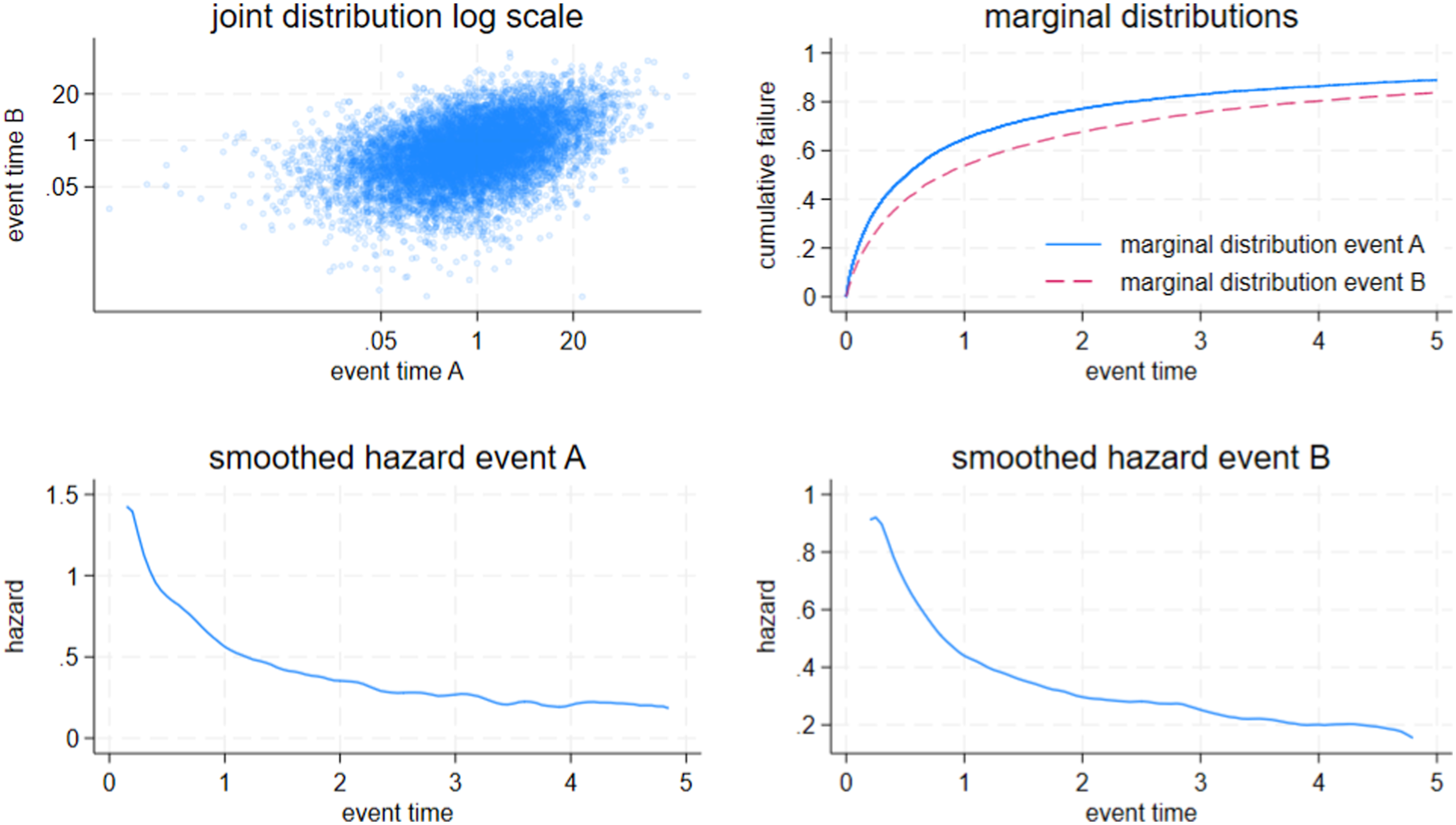

The upper left panel displays the joint distribution on a log-log scale. We use the log-log scale because both distributions are skewed to the right. The axes display the event times .05, 1.0, and 20. The data points have a moderate correlation: .31. This is considerably less than ρ = .75 because randomness attributable to the exponential distribution dilutes the correlation. In this paper, we will be concerned with estimating a joint distribution analogous to the top left panel in Figure 1 and we will be concerned with interpreting the overall correlation between events A and B. In our application, A will be the event returning to prison for nuisance recidivism and B will be returning to prison for pernicious recidivism. Additionally, in our application, a person can complete supervision with neither event A nor B occurring (event Z), and in the terminology of survival models, such a person is censored at the end of the risk period.

The upper right panel displays the marginal distribution for events A and B. The marginal distributions are derived from the joint distribution. In this paper, we will be especially interested in estimating these marginal distributions because they represent the underlying stochastic processes accounting for the timing for occurrence of events A and B.

The lower two panels represent smooth hazards. (Crudely, the hazard is the instantaneous probability of failure given that a person has not failed up to that time.) Their shapes may be surprising given that the marginal distributions were assumed to be exponential, and the exponential is known to have a constant hazard. The explanation is that the exponential/normal mixture reshapes the exponential hazard (Heckman & Singer, 1984). Thereby, the normal mixture has two effects: inducing a correlation between the timing of the two events (unless ρ = 0) and reshaping the hazard (regardless of ρ).

Figure 1 introduced familiar survival concepts. Determining the joint distribution, the marginal failure functions, and the hazards is straightforward given observed values of t_A and t_B, the failure times for event A and event B, respectively. But the problem we face is that we can only observe the event that occurred first, so we observe t_A if t_A < t_B, and we observe t_B if t_B < t_B. In this regard, the events are said to be competing. Competing events require introducing new, potentially unfamiliar concepts. See Figure 2.

Figure 2.

Curves are based on simulated data from exponential/normal mixtures. Panel 1 displays empirical distributions for the overall failure function and for the two cumulative incidence functions. Panels 2 and 3 display empirical marginal distributions, as well as estimated marginal distributions that assume independence between the two events. The estimates are poor.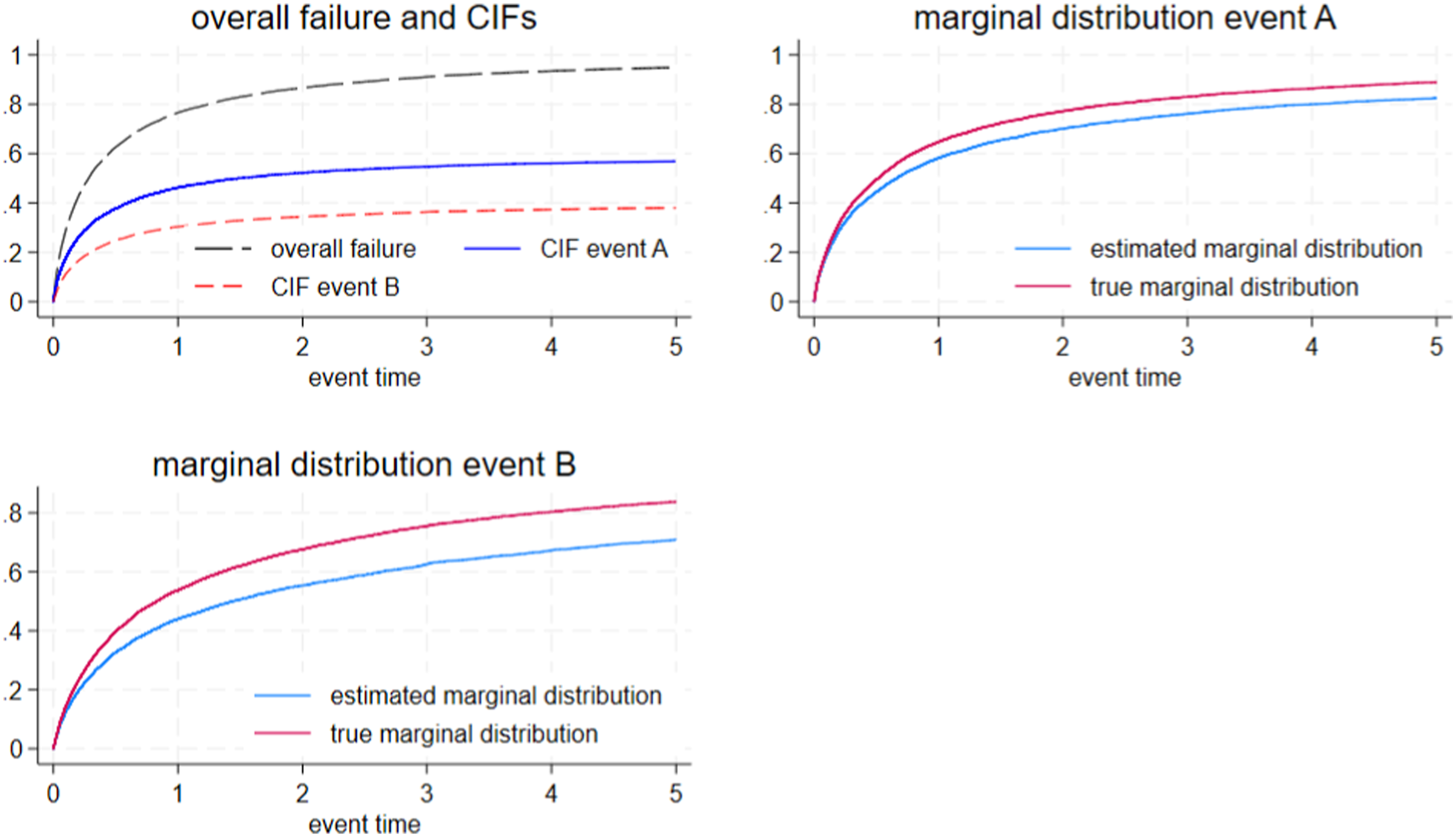

The upper left panel of Figure 2 displays three curves. The overall failure function is the cumulative distribution of any failure—event A if it occurs first and event B if it occurs first. The overall failure function is what criminal justice researchers estimate when they do not distinguish recidivism by seriousness.

The first panel also displays the cumulative incidence functions (CIFs). CIFs are commonly used in epidemiology and biomedical research, but not much to our knowledge in criminal justice research. The CIF for event A is the empirical distribution of event times we would observe if we only recorded t_A when t_A < t_B, and otherwise, we let time continue with no recorded event. The CIF for event B is the empirical distribution of event times we would observe if we only recorded t_B when t_B < t_A. If the occurrence of event B prevents event A from occurring, then the CIF for A reflects the distribution of type A events that actually occurred, and vice versa. Note that the CIFs are not proper distributions because they never reach one. Note also that the sum of the two CIFs equals the overall failure function. The overall failure function and the cumulative incidence functions can be estimated using commonly available software (Cleves et al., 2010; Lambert, 2017), and importantly, we can estimate these functions without knowing the joint distribution or ρ.

The remaining panels redisplay the two marginal distributions as well as estimates of those marginal distributions using a Kaplan–Meier non-parametric estimator. The estimates are poor, a consequence of the Kaplan–Meier estimator assuming that the two events are independent when they are not. Parametric and partially parametric estimators have the same deficiencies when faced with dependent censoring.

Unbiased estimation of the marginal distributions requires that we account for the dependence between the two events, and that requirement brings us back to estimating the joint distribution. Regrettably, the parameters of the joint distribution are not identified for the problem posed above (Tsiatis, 1975). Intuitively, we can observe the occurrence of event A, or we can observe the occurrence of event B, but we can never observe their joint occurrences so we cannot estimate ρ. As van den Berg (2010, p. 7) observed: “…without additional structure, each dependent competing risks model is observationally equivalent to an independent competing risks model. The marginal distributions in the latter can be very different from the true distributions.”

The problem, then, is to find the additional structure, which comes from adding covariates to the model. Extending the work of Heckman and Honore (1989), van den Berg (2010, p. 8) summarizes: “Somewhat loosely, X has two continuous variables that are not perfectly collinear and that act differently on θ₁ and θ₂. … identification is not based on exclusion restrictions of the sort encountered in instrumental variables analysis, which require a regressor that affects one endogenous variable but not the other. Here all explanatory variables are allowed to affect both duration variables – they are just not allowed to affect the duration distributions in the same way.”

The proof of this assertion is complex, and intuition is lacking. An extension of the simulation provided above may be helpful. As above, we use an exponential/normal mixture, but we add covariates. Write $λ_{A} = \exp (β_{10} + β_{11} x_{1} + β_{12} x_{2} + 1.5 u_{1})$ and $λ_{B} = \exp (β_{20} + β_{21} x_{1} + β_{22} x_{2} + 1.5 u_{2})$ . The variables x₁ and x₂ are both distributed as independent uniform, but this choice is not important provided they are not collinear. As before, u₁ and u₂ are distributed as standard bivariate normal. We will modify the values of β to illustrate points.

We began with β₁₀ = 0; β₁₁ = 2; β₁₂ = 1; β₂₀ = 0; β₂₁ = 1; and β₂₂ = 2. Using these parameters, we simulated 10,000 observations and attempted to fit the model using maximum likelihood. After failing to find acceptable starting values, Stata’s maximum likelihood routine aborted, an indication that the model is not well identified. Following a recommendation by Emura and Chen (2018), we computed a profile likelihood. Specifically, the upper left panel (model 1) of Figure 3 displays minus the mean likelihood for a range of values for ρ. The curve’s minimum has the highest likelihood. The profile likelihood suggests that ρ is close to .8, not far from the .75 value built into the simulation.

Figure 3.

Illustrative profile likelihoods: Minus the mean likelihood for simulations based on the exponential/normal mixture model with two covariates. The effect of the two covariates falls from the upper left panel to the lower right panel.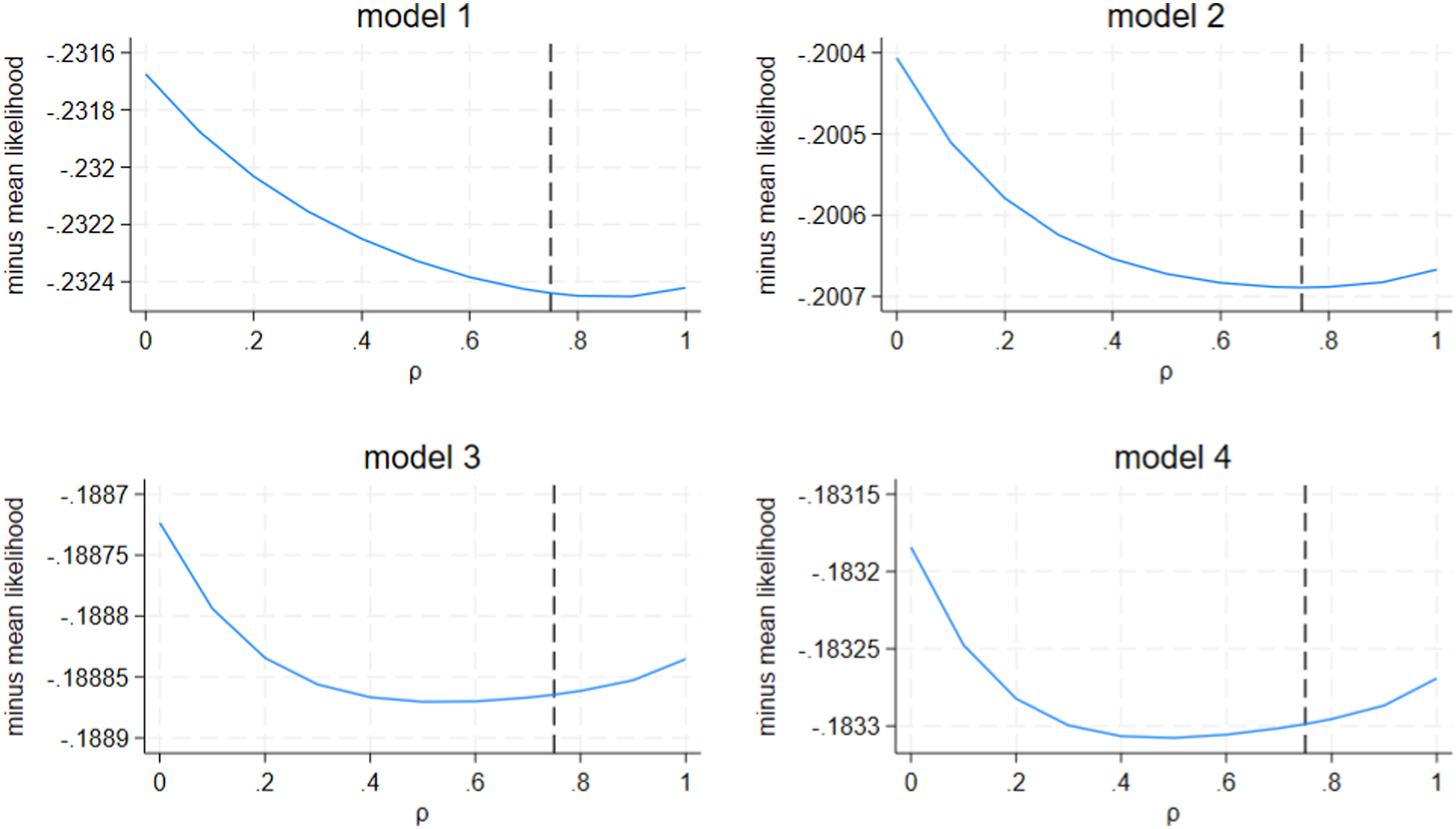

We repeated this exercise for different values of β: For model 2, β₁₀ = .75; β₁₁ = 1; β₁₂ = .5; β₂₀ = .75; β₂₁ = .5; and β₂₂ = 1. For model 3, β₁₀ = 1.12; β₁₁ = .5; β₁₂ = .25; β₂₀ = 1.12; β₂₁ = .25; and β₂₂ = .5. And for model 4, β₁₀ = 1.34; β₁₁ = .2; β₁₂ = .2; β₂₀ = 1.34; β₂₁ = .1; and β₂₂ = .2. The constants change so that the average values of λ₁ and λ₂ remain about the same across simulations. The other β’s become smaller so that the x’s have decreasing effects across the four scenarios. Interest is in the consequences of these decreasing effects.

In panels 1 and 2, the profile likelihoods achieve a minimum very near the true value of .75. However, the likelihood is flat within the range .6 ≤ ρ ≤ .8. The difference between the maximum and minimum mean loglikelihood is only 2.618 × 10⁻⁵ for model 1 and 6.4 × 10⁻⁶ for model 2. Likely this explains why Stata was unable to establish acceptable starting values when ρ was unconstrained. In contrast, the profile likelihoods for models 3 and 4 do a poor job of identifying the known value of ρ. The profile likelihoods for both suggest ρ = .5, but the profile likelihoods are flat across a broad range. The simulation results suggest that identification depends importantly on the covariates having a significant impact on the timing until recidivism.

Note in model 1 that β₁₁≠β₂₁ and β₁₂≠β₂₂. This is consistent with the identification requirement that the covariates must have different effects on the timing of recidivism. To violate the condition, set them equal so that β₁₁ = β₂₁ = 2 and β₁₂ = β₂₂ = 1. We do not draw the profile likelihood, but it looks similar to the lower two panels of Figure 3. The profile likelihood is flat and the best estimate for ρ is about .5.

These simulations illustrate conditions affecting identification of the joint distribution. There must be covariates; they must have an appreciable impact on the marginal failure rates; and the covariates must affect the marginal distributions differently. Of course, no simulation substitutes for mathematical proof, but the simulations illustrate conditions that can be formally proved.

Critics have expressed skepticism regarding this solution. For example, van den Berg (2010) observes that “… there is substantial evidence that estimates are sensitive to misspecification of functional forms of model elements ….” In response, we follow the advice of Cameron and Trivedi (2005, pp. 619–620), who recommend using flexible parametric approaches. We will present our model subsequently.

We provide diagnostic tests, namely, if our model of the joint distribution and the marginal distributions is adequate, we should be able to use simulated data based on the bivariate distribution to approximate the overall failure function and the CIFs when those are estimated using standard estimators.

The Model

Given its simplicity, the exponential/normal mixture is useful for illustrating concepts important for this study, but because of that simplicity, the exponential is not useful for application. Importantly, as shown in Figure 1, the hazard for the exponential/normal mixture decreases monotonically over time. But evidence is that the hazard during PCCS first increases and then falls continuously (Dejong, 1997; Kurlychek et al., 2012; Petersilia, 1997; Schmidt & Witte, 1987).

A better model is a Weibull/normal mixture. The Weibull is a two parameter (λ and κ) distribution with hazards that increase monotonically when κ > 1, that are flat when κ = 1, and that decreases monotonically when κ < 1. For the Weibull/normal mixture, we can rewrite the λ by including the normal variate as we did for the exponential. This can change the monotonicity of the hazards as we illustrate below.

As before, there are two events—event A and event B—whose failure times have a joint distribution, but now the two marginal distributions are Weibull/normal mixtures. Assume that event A has a mixture distribution with parameters $λ_{A} = e^{θ_{A} + u_{A}}$ and κ_A. Let $θ_{A} = \ln (1.25)$ ; let κ_A = 2.0; let $u_{A}$ be distributed as normal with $μ_{A} = 0$ and $σ_{A} = 1.5 .$ Similarly, assume that event B has a mixture distribution with parameters $λ_{B} = e^{θ_{B} + u_{B}}$ and κ_B. Let $θ_{B} = \ln (0.75)$ ; let κ_B = 2.0; let $u_{B}$ be distributed as normal with $μ_{B} = 0$ and $σ_{B} = 1.5 .$ Furthermore, assume that $u_{A}$ and $u_{B}$ are distributed as bivariate normal with correlation ρ = .75. Given these assumptions, Figure 4 displays distributions and hazards based on the simulated data.

Figure 4.

Curves are based on simulated data from Weibull/normal mixtures. Panels 1 and 2 are empirical distributions based on simulated data. Panels 3 and 4 are estimates of the hazards using a Kaplan–Meier estimator.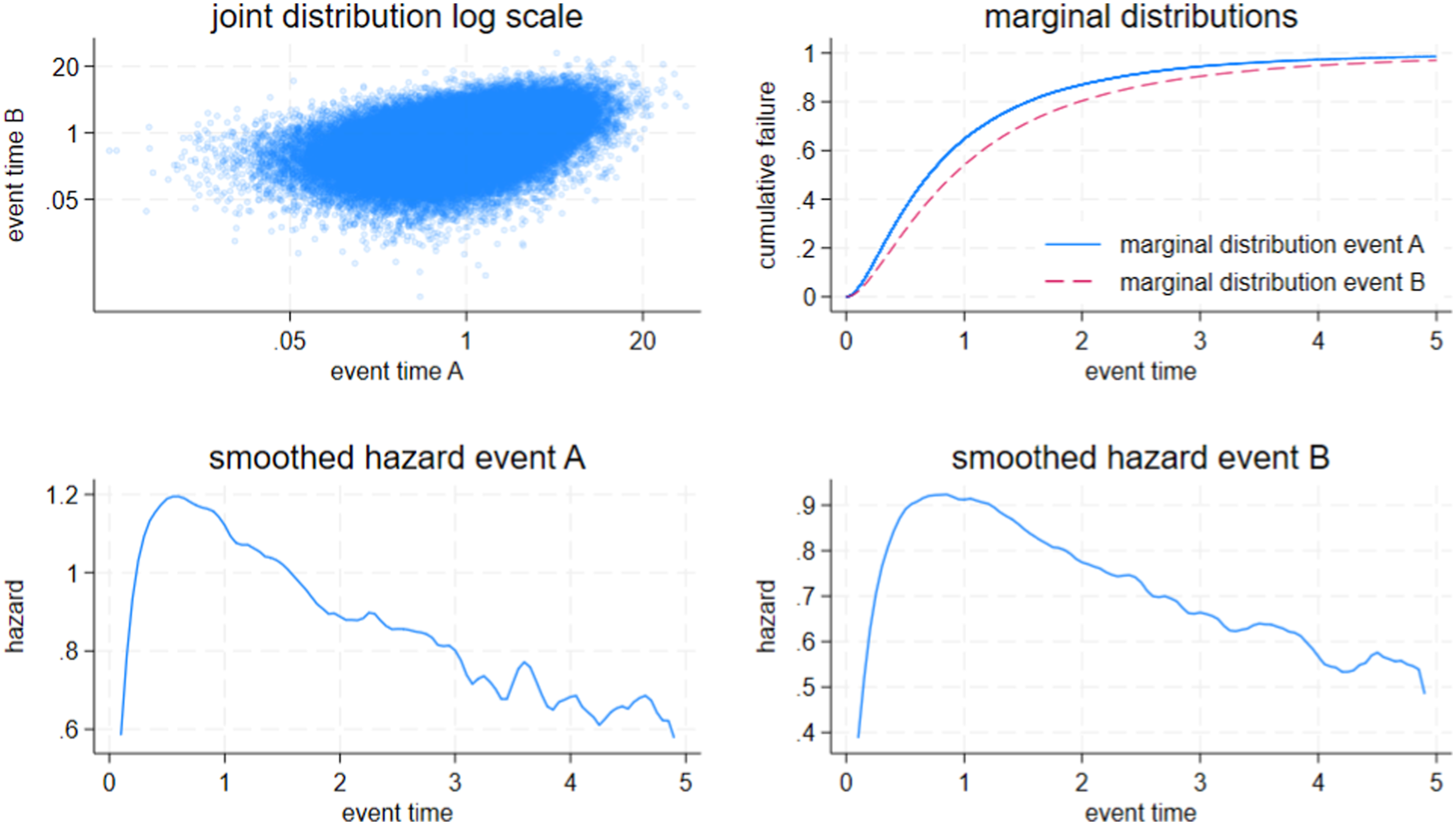

Figure 4 (Weibull/normal mixture) is the counterpart to Figure 1 (exponential/normal mixture). We draw attention to the bottom panels, which display smoothed hazards. There are irregularities in the smoothed hazards. Irregularities are characteristic of Kaplan-Meier estimates. Ignoring these irregularities, given κ > 1, the hazards increase to a peak and then decreases monotonically over the range of interest. Therefore, the Weibull/normal mixture can capture the shape of hazards that we expect based on a literature scan.

The literature also suggests that an appreciable proportion of FIPs will never return to prison (Rhodes, Gaes, et al., 2014). That observation suggests introducing a split-population model (Schmidt & Witte, 1988), sometimes called a cure model in biomedical statistics. Specifically, a proportion P of FIPs have no chance of experiencing recidivism over an infinite length risk period. In the criminal justice literature, they are said to desist (National Institute of Justice, 2021). The complement 1-P will have event times drawn from the distribution in the upper left panel of Figure 4. Given a split-population specification, the other three panels of Figure 4 display the distribution of outcomes for the population members who draw outcomes from the joint distribution.

The illustrations have assumed considerable homogeneity across the population of FIPs. We now adopt a vector of covariates X and assume that parameters (excluding the σ’s) are functions of these covariates

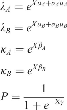
\begin{array}{l} λ_{A} = e^{X α_{A} + σ_{A} u_{A}} \\ λ_{B} = e^{X α_{B} + σ_{B} u_{B}} \\ κ_{A} = e^{X β_{A}} \\ κ_{B} = e^{X β_{B}} \\ P = \frac{1}{1 + e^{- X γ}} \end{array}

The u_A and u_B are distributed as standard bivariate normal. Exponentials are used when parameters must be positive.

The marginal failure function is written $F (t) = 1 - e^{λ t^{κ}}$ . Taking the derivative of F(t) shows that time until failure increases with λ and increases with κ. This observation provides some interpretation to the α, β, and γ sub-parameters.

Diagnostics

Inferences rest on a host of assumptions. We discuss sensitivity and diagnostic tests in this section and demonstrate later that our model meets these tests.

The parameter ρ is difficult to estimate. A prudent step is to estimate the model conditional on a justifiable range for ρ. Following suggestions by Emura and Chen (2018) we use a profile likelihood for this exercise. We consider this the first diagnostic test.

Additional diagnostic tests provide reassurance that the estimated marginal failure functions are reasonable. If we treat overall failure as the outcome “A or B is observed,” then we can estimate the overall failure function, which is identified using a Kaplan–Meier estimator. But we can also infer the overall failure function using the estimated marginal failure functions. If the estimate and inference are much different, we would conclude that the estimated marginal failure functions are inadmissible. Thus, we have the second diagnostic tool.

We can estimate the cumulative incidence function (CIF) directly using a Coviello and Boggess (Coviello & Boggess, 2004) estimator. We can also infer the CIF using the estimated marginal failure functions. If the CIF based on the marginal failure functions are unlike the Coviello and Boggess estimator, we would judge the estimated marginal failure functions as inadmissible. Thus, we have a third diagnostic test.

A different type of evaluation test is to ask whether parameter estimates are qualitatively consistent with expectations. For example, we expect past criminal history to have a strong association with recidivism (Gendreau et al., 1996). Every x (an element of X) affects every parameter except σ, so it is difficult to interpret the effect of x on recidivism by inspecting how x affects the α, β, and γ parameters. A workable approach is to simulate time until failure using the estimated marginal failure functions and then use a simple survival model (a Cox regression, e.g.,) to summarize the effect of X on failure using the simulated data. This approach provides a simple summary of how each x affects the outcomes. If the parameter estimates differed qualitatively from expectations, we would question the model.

Finally, as a sensitivity test of the marginal failure distributions, we estimate a competing events model using a Gaussian copula with flexible marginal distributions based on restricted cubic splines. A copula is a function that ties two marginal distributions together so that the marginal distributions are correlated (Emura & Chen, 2018; Trivedi & Zimmer, 2005). Conditional on covariates, the copula’s single parameter determines the correlation.

Linear splines—familiar to most readers—are used to approximate nonlinear curves. To assure greater flexibility, cubic splines replace linear lines with polynomials of the form ${δ_{0} + δ}_{1} t + δ_{2} t^{2} + δ_{3} t^{3}$ . The parameters change at breakpoints—t₁, t₂, t₃, etc. To assure smooth representations, the parameters are restricted so that the lines join, have common first derivatives, and have common second derivatives, at the break points. Often just one or two breakpoints are sufficient. To apply cubic splines, we adopt Royston–Parmer models (Royston & Lambert, 2011; Royston & Parmar, 2002). We wrote a Stata-based likelihood procedure that introduces R–P models into a Gaussian copula using the likelihood specified by Emura and Chen. If the marginal distributions in our split-population Weibull mixture are inadequate, we would expect this inadequacy to be diagnosed by the copulas providing a much better fit to the data.

This comprises a great deal of diagnostic testing. We will show that diagnostic testing supports accepting the split-population Weibull mixture model as a good representation of nuisance and pernicious recidivism.

Data

Data are from the National Corrections Reporting Program (NCRP), sponsored by the Bureau of Justice Statistics. For several states, the NCRP reports all prison and post-confinement community supervision (PCCS) terms experienced by a person over many years. We use data from New York State for this investigation.

New York has a mixed system for determining prison release and parole length (Reitz et al., 2020). Many offenders are sentenced to a fixed prison term followed by a judicially imposed post-release term of community supervision. Other offenders are sentenced to indeterminate terms. For them, release is determined by the parole board or by the department of corrections. The NCRP reports release categories as parole (41.6%), mandatory release (39.7%), other conditional (.6%), and expiration (15.1%). About 2.9% of releases do not fall into any of these categories—deaths, transfers, etc. For our purposes, anyone who served a post-release period of supervision entered the analyses because they qualified as having competing risks.

PCCS terms are finite. The NCRP reports when prison and PCCS terms began and ended (or that they were ongoing as of the end of 2019). The NCRP reports how a term began and how it ended. We selected all PCCS terms that began between 2006 and 2019 inclusive that satisfied the criterion: The PCCS term had to be preceded by a prison term. Over 95% of PCCS terms met this criterion. We determined the distinction between prison returns for nuisance behaviors and returns for pernicious behaviors using PCCS release codes. These were supplemented with prison admission codes when PCCS release codes were missing.¹ The release codes appear accurate when compared with separate administrative reports from the Bureau of Justice Statistics (Oudekerk & Kaeble, 2021). For example, the NCRP reports 19,604 PCCS releases in 2017; the BJS report lists 19,519. The small difference can be attributable to slightly different methods of assigning the release date. BJS and the NCRP agree that 56.1%/54.5% of terms ended successfully, that 6.4/6.3% ended with a new sentence, and that 36.0/35.9 ended with a revocation but no new conviction. (About 1.5/1.7% were deaths.) Another quality control check was to assure that prison authorities and parole authorities agreed about why an offender exited prison and entered PCCS, and why an offender exited PCCS and entered prison, according to the NCRP. There was broad agreement. Measures of concordance and additional data assembly steps are described in a separate memo available from the authors.

After all data processing steps, 290,179 supervision terms entered the analysis. For each term, we assembled the following covariates used to predict outcomes. See Table 1.

Table 1.

Covariates Entering the Analysis. All Covariates are Categorical Except Interaction, Seriousness, and Trend.

	Mean	sd	Min	Max
educ8	.310	.462	.000	1.000
educ9	.116	.321	.000	1.000
educ10	.164	.370	.000	1.000
educ11	.141	.348	.000	1.000
educ12	.229	.420	.000	1.000
some_college	.036	.187	.000	1.000
College	.004	.061	.000	1.000
Hispanic	.234	.423	.000	1.000
Male	.932	.252	.000	1.000
White	.343	.475	.000	1.000
Black	.533	.499	.000	1.000
CH1	.089	.285	.000	1.000
CH2	.135	.342	.000	1.000
CH3	.072	.258	.000	1.000
CH4	.053	.223	.000	1.000
CH5	.039	.194	.000	1.000
CH6	.031	.175	.000	1.000
CH7	.026	.161	.000	1.000
CH8	.024	.153	.000	1.000
CH9	.018	.134	.000	1.000
CH10	.072	.258	.000	1.000
25 or younger	.145	.352	.000	1.000
26–35	.356	.479	.000	1.000
36–45	.262	.440	.000	1.000
46–55	.176	.381	.000	1.000
56 or more	.061	.239	.000	1.000
Interaction	.107	.309	.000	1.000
Seriousness	6.547	.499	.000	8.400
Trend	.475	.290	.000	1.000

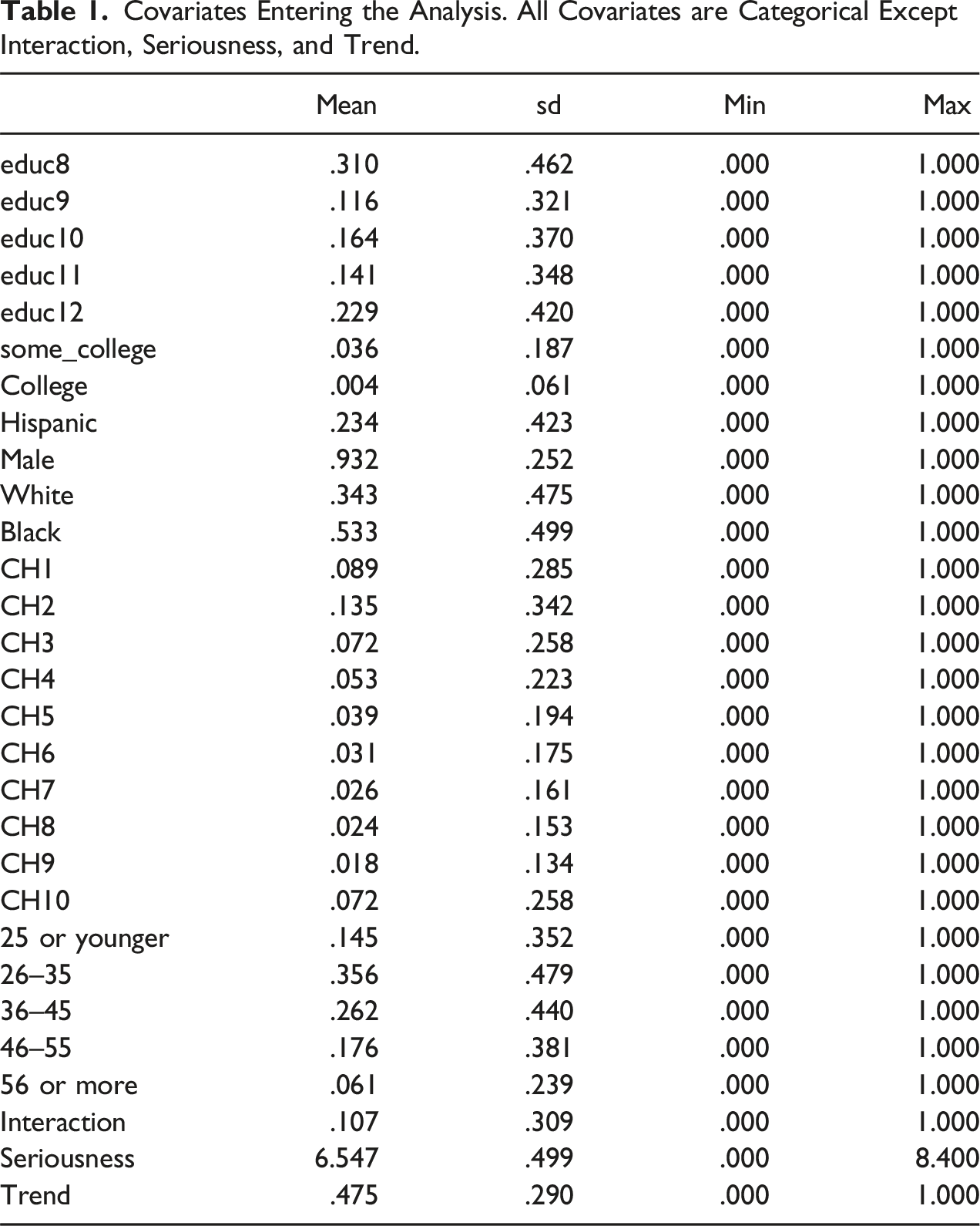
Age is age when supervision began. It is represented as ordered categories. Male distinguishes offenders by sex. Race is distinguished as white, black, and other. Hispanic distinguishes Hispanics from non-Hispanics.

Criminal history is constructed from NCRP prison terms. Because all offenders were in prison prior to release, and hence a variable indicating any prior prison stay would be collinear, the prison stay leading to PCCS was ignored when constructing the criminal history categories. Otherwise, CH1 means that the offender had been released from prison for a previous conviction within one year of readmission to community supervision. CH2 means that the offender had been released within two years but longer than one year. The CH variables range from CH1 to CH10. The category CH10 includes all releases more than 9 years in the past. A base category is no prior prison terms within 10 years of parole admission. Because the prison stay leading to parole was ignored when constructing the criminal history category, the “no prior prison term” category (one minus the sum of the CH variables) predominates.

The variable “seriousness” is the logarithm of the seriousness of the offense leading to the prison term prior to parole. Based on the BJS_OFFENSE_1 code, it is the median time served by all offenders who completed an original prison sentence for that BJS_OFFENSE_1 code, generally the conviction offense leading to the longest sentence. We used a logarithm because the variable is highly skewed. A final variable is a trend variable defined by date of admission to community supervision. The trend is rescaled to run from 0 (the earliest admission date) to 1 (the latest admission date). Rescaling assists model convergence.

The variables are imperfectly measured. Consider the CH codes. First, it is impossible for us to reliably observe prison terms that ended more than ten years before admission to parole, because New York NCRP data do not extend beyond ten years for individuals who entered supervision early in the data observation window. Likely this introduces only a minor distortion because offenders seldom return to prison after so long of a period at liberty (Rhodes, Gaes, et al., 2014). A larger problem is that younger offenders are typically unable to acquire past prison terms partly because juvenile records are hidden. Therefore, we introduced an interaction between the youngest age category (25 and younger) and the category “no prior prison.” Because we could observe earlier prison terms for older age categories, additional interaction terms seemed unnecessary.

Estimation and Diagnostic Tests

Using the model and data described in the previous section, we estimated the parameters for the joint distribution. Based on diagnostic tests, reported immediately below, we judge the estimation as adequate.

Profile Likelihood

The marginal hazards are not well identified but can be bounded. We begin by estimating the profile likelihood for the parameter ρ. See Figure 5. To estimate the profile likelihood, we adopt incremental values for ρ, estimate the model conditional on each ρ, and record the log-likelihood values. To facilitate reading the figure, we report minus the loglikelihood values divided by the number of observations. Therefore, the best choice for ρ is a value that minimizes (not maximizes) the function in Figure 5. For our purposes, narrower steps and greater granularity seemed unnecessary.

Figure 5.

Profile likelihood. Dots represent the mean loglikelihood as a function of assumed values of ρ. Two values (ρ = .6 and ρ = .8) are approximations because the likelihood did not converge in 25 iterations.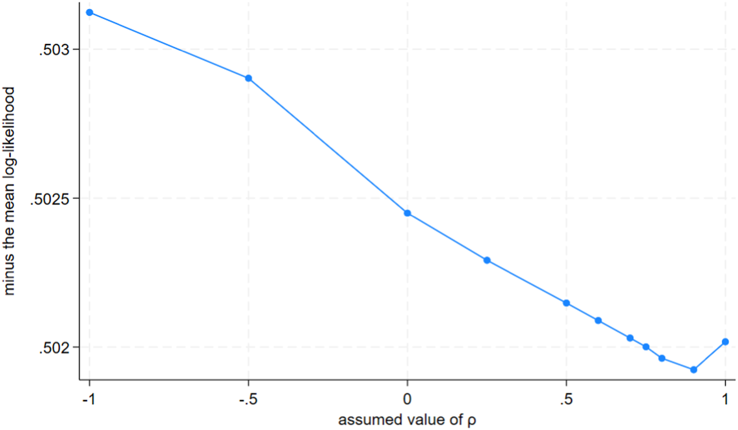

The figure illustrates why the competing events model is so difficult to identify. Although the “best” value for ρ appears to be about .90, the profile likelihood is fairly flat between ρ = 1.0 and ρ = .70. While a direct estimate of ρ might settle on a value near .9, the estimate would have a high standard error and we would have little confidence in the estimate. Although the value of ρ is imprecisely identified, Figure 5 suggests that ρ is almost certainly larger than 0, because there is a large jump from ρ = .0 to ρ = – .5; it is highly likely to exceed .5, because there is a modest but appreciable jump from .5 to smaller values of ρ; and there is a strong likelihood that ρ approaches one. We use values of ρ = .0, .5, and 1.0 to bound estimates.

Inferred Values for the Overall Failure and for the Cumulative Incidence Functions

Using the parameter estimates for the full model, we simulated the failure times for the two estimated marginal failure distributions.² In Figure 6, we draw the estimated marginal failure functions based on different assumptions about ρ. The first panel shows the estimated marginal failure functions for nuisance recidivism conditional on three assumed values of ρ: ρ = .0, .5, and 1.0. Similarly, the second panel shows the marginal failure functions for pernicious recidivism. For New York, the marginal failure functions for nuisance are relatively insensitive to assumptions about ρ, but the marginal failure functions for pernicious recidivism are comparatively sensitive to assumptions about ρ. Comparing the first two panels, we see that nuisance recidivism tends to occur much earlier than pernicious, explaining why the effect of ρ is larger for pernicious recidivism than for nuisance recidivism: nuisance recidivism frequently interrupts pernicious, but pernicious recidivism less frequently interrupts nuisance recidivism.

Figure 6.

Estimated marginal failure functions for nuisance recidivism and pernicious recidivism for different values of ρ (Panels 1 and 3) and implied overall failure function (Panel 3).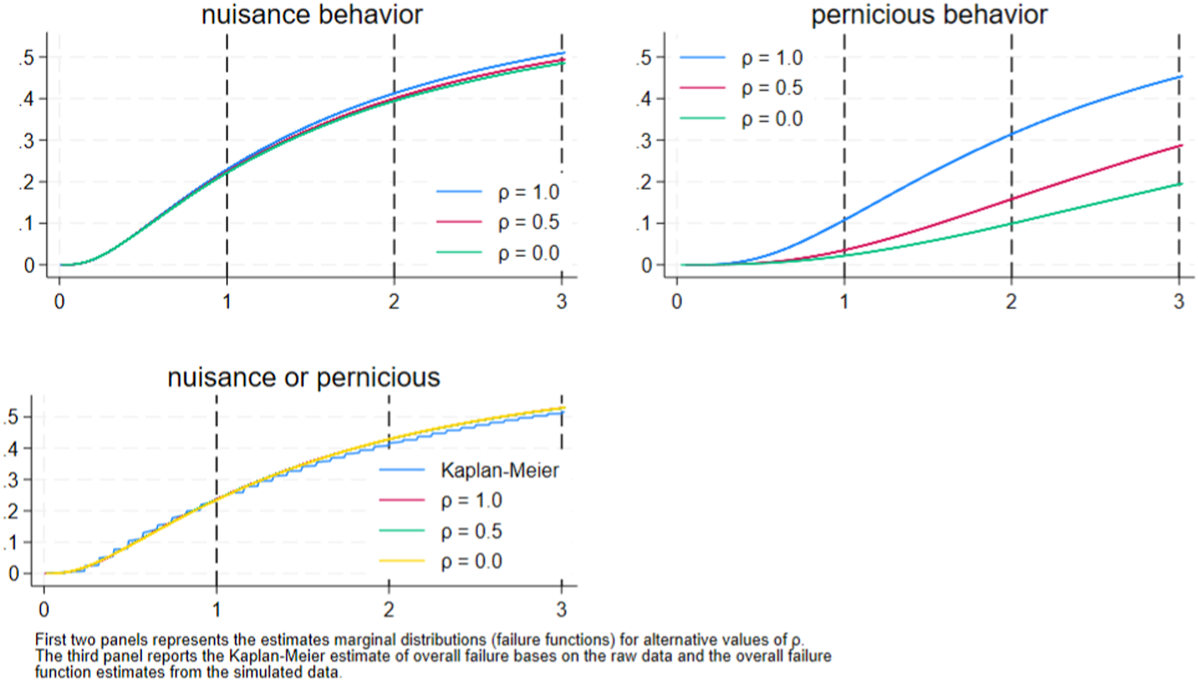

A third panel shows the overall failure functions inferred from the estimated marginal failure functions shown in the first two panels. Regardless of the assumed value of ρ, every pair of marginal failure functions should produce the same overall failure function. Thus, we expect these overall failure functions to be indistinguishable, and that is true. They blend into a single line. We also estimated the overall failure function using a Kaplan–Meier estimator. We expect the K–M failure function to be like the three overall failure functions inferred from the estimated marginal failure functions. Expectations are met. Although the K–M estimator is distinguishable from the overall failure functions based on the marginal failure functions, the departure is modest, suggesting that our split-population Weibull mixture model adequately fits the data.

Again, using simulated data derived from the estimated marginal failure functions, we draw the inferred cumulative incident functions (Figure 7). The first panel shows the CIF for nuisance recidivism. There are three lines, each derived from the three estimated pairs of marginal failure functions. As expected, because the pairs of marginal failure functions should produce the same cumulative incidence functions, the three versions of the cumulative incidence function for A are virtually the same. The second panel shows the three CIFs for pernicious recidivism. Again, the three lines are virtually indistinguishable. As expected, the different marginal failure functions give rise to the same cumulative incidence functions. A third panel shows the overall failure function. At any fixed failure time, adding the two cumulative incidence functions should produce the overall failure function. An eyeball test shows that this property holds. And a fourth panel shows the Coviello and Boggess estimator of the CIF for the pernicious recidivism. The curves in the second and fourth panels should agree. An eyeball test confirms that they do.

Figure 7.

Inferred cumulative incidence function for nuisance recidivism and pernicious recidivism (labeled B in panel 4) for different values of ρ (Panels 1 and 2); inferred overall failure time (Panel 3); and the Coviello and Boggess estimator for pernicious recidivism (Panel 4).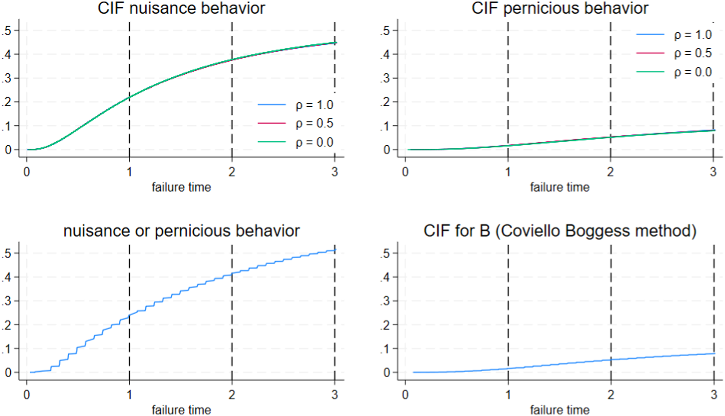

The split-population Weibull mixture model passes this set of diagnostic tests. The tests say nothing about the choice of ρ. Given a value of ρ based on the profile likelihood, the tests do suggest that the split-population Weibull/normal mixture model fits the data sufficiently well to replicate the overall failure distribution and the cumulative incidence functions, both of which can be estimated independently of the split-population Weibull/normal mixture model.

Inspecting the Parameter Estimates

Both λ′s, both κ′s, and the P have as many parameters as there are independent variables plus a constant. There are additional parameter estimates for the σ′s. Furthermore, there are separate estimates for different assumptions about ρ. The complete table of parameter estimates (slopes and standard errors for ρ = .0, .5, and 1.0) appears in a Supplemental Appendix, but because the table is so difficult to interpret, we pay it little attention beyond a few general observations.

First, we note that the estimated values of σ vary with assumptions about ρ, but the values of σ are always large. “Large” can be judged by comparing the role of other covariates after considering that the σ are parameters scaling a standard normal distribution. Unmeasured heterogeneity is definitely an important factor determining the outcomes. Possibly this unmeasured heterogeneity is a consequence of our data missing important covariates, but it may be partly a consequence of model misspecification.

Second, we observe that parameters tend to be qualitatively the same regardless of the assumed value of ρ. In fact, for the most part, the magnitude of the parameters does not vary greatly with the assumed values of ρ. “Greatly” is a subjective term, but different assumptions about ρ do not materially alter impressions of how different covariates affect the hazards.

Third, the parameters for nuisance recidivism have lesser variation with respect to ρ than do the parameters for pernicious recidivism. Presumably, this occurs because the process leading to pernicious recidivism infrequently interrupts the process leading to nuisance recidivism, while the process leading to nuisance recidivism frequently interrupts the process leading to pernicious recidivism. Because of less censoring, the marginal failure function for nuisance recidivism is better identified than the marginal failure function for pernicious recidivism.

The above observations aside, it is difficult to judge how any single covariate affects the processes leading to nuisance or pernicious recidivism. To assist with interpretation, we used the estimated parameters reported in the Supplemental Appendix Table to simulate the time to failure according to the estimated marginal failure functions. Then, using the simulated data for nuisance behavior, we estimated Cox models where the occurrence of nuisance behavior was the dependent variable. Note that this is just a convenient way of summarizing the marginal failure functions using an easy to interpret statistical procedure.

Based on simulation data from the marginal failure function for nuisance recidivism, columns (1), (2), and (3) of Table 2 show results from the Cox model. Based on simulated data for pernicious recidivism, columns (4), (5), and (6) show results from the Cox model. The Cox model provides no estimate for σ, whose effect would be captured as part of the baseline hazard.

Table 2.

Parameter Estimates From a Cox Regression on Simulated Data by Event Type and Assumptions About ρ.

Variables	Nuisance Behavior (A)			Pernicious Behavior (B)
	(1)	(2)	(3)	(4)	(5)	(6)
	ρ = 1.0	ρ = .5	ρ = .0	ρ = 1.0	ρ = .5	ρ = .0
educ8	.289***	.211***	.171***	.122	−.275***	−.371***
educ9	.327***	.254***	.217***	.167***	−.240***	−.366***
educ10	.312***	.230***	.211***	.136	−.305***	−.404***
educ11	.265***	.208***	.175***	.102	−.280***	−.368***
educ12	.0768	−.00346	−.0287	−.151***	−.618***	−.686***
some_college	−.00572	−.0604	−.0860	−.185***	−.510***	−.576***
Hispanic	−.352***	−.358***	−.359***	−.301***	−.171***	−.112***
Male	.226***	.202***	.189***	.369***	.561***	.640***
White	.131***	.120***	.111***	.173***	.206***	.227***
Black	.00757	−.00716	−.00980	.0754***	.169***	.243***
CH1	1.595***	1.619***	1.599***	1.741***	1.693***	1.429***
CH2	1.419***	1.426***	1.415***	1.517***	1.468***	1.276***
CH3	1.105***	1.116***	1.097***	1.180***	1.148***	.989***
CH4	.913***	.927***	.887***	1.024***	1.071***	.999***
CH5	.788***	.811***	.768***	.891***	.976***	.926***
CH6	.672***	.677***	.637***	.761***	.865***	.812***
CH7	.607***	.606***	.577***	.730***	.818***	.756***
CH8	.568***	.593***	.549***	.661***	.694***	.704***
CH9	.556***	.513***	.488***	.617***	.701***	.618***
CH10	.291***	.296***	.266***	.294***	.300***	.266***
25 or younger	.446***	.429***	.444***	.513***	.649***	.728***
26–35	.469***	.468***	.470***	.470***	.452***	.473***
36–45	.398***	.405***	.417***	.391***	.386***	.378***
46–55	.296***	.287***	.309***	.317***	.345***	.362***
Interaction	.602***	.592***	.540***	.685***	.692***	.651***
Seriousness	−.173***	−.164***	−.155***	−.171***	−.189***	−.234***
Trend	.0769***	.105***	.117***	.0919***	.129***	.0782***
Observations	290,025	290,025	290,025	290,025	290,025	290,025

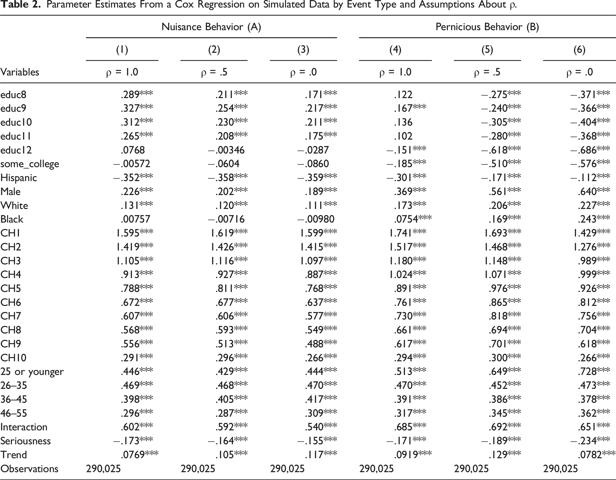
A parameter of less than zero decreases the failure rate; a parameter equal to zero is neutral; and a parameter greater than zero increases the failure rate. Estimated parameters are sometimes relative to an omitted category. For age and criminal history, the omitted category is difficult to discern because of the interaction between the youngest age category and criminal history. It is also helpful to read down the table for a continuous variable that has been recoded using ordered categories.

Generally, variables that accelerate the time to nuisance recidivism also accelerate the time to failure for pernicious recidivism. For example, looking at the education variable, we see that failure rates tend to fall as education increases. The pattern is not perfect, but higher education tends to predict lower failure rates of both types. The omitted category is college graduate, which seems to have an unexpectedly larger hazard. However, college graduates are less than one-half of one percent of all parolees (see Table 1), so the estimate for college graduates is exceptional and probably unreliable.

Similarly, more recent prison terms accelerate both events. Failure seems to decline with age, but the pattern is obscured by the interaction between the youngest age category and no prior prison. Over time, there is a trend toward more failures, but given that time is recoded to run from zero to one, that trend is small although not immaterial given its impact on the hazard. Supervisees incarcerated for more serious crimes tend to have lower return rates.

Generally, parameter estimates conform to expectations. This observation is reinforced by evidence from the next section.

Sensitivity Tests Using a Gaussian Copula With Flexible Marginal Distributions

Using the same data, we estimate a model with a Gaussian copula with marginal failure distributions based on Royston–Parmer cubic spline models. We employed what Royston–Parmer called the theta model, which is the most general of their models. We estimated models based on one, two, and three knots for the restricted cubic spline. Based on this testing, we adopted a model with three knots. The log-likelihood was −290,360. Using a BIC or AIC criterion, this copula model was inferior to the split population model with a Weibull/normal mixture. Its likelihood was −144,876 (ρ = 1.0), −144,920 (ρ = −.5), and −145,015 (ρ = .0). Sensitivity testing suggests that our choice of the split-population Weibull/normal mixture model is justified, or at least superior to the copula with marginal failure functions based on restricted cubic splines.

We previously simulated data using the estimated marginal failure distributions and then used a Cox model to summarize. The summary was reported in Table 2. We can compare these parameters with parameters from the copula. The comparison cannot be direct, because the different parameterizations lead to different parameters with the same marginal effects. To allow a comparison, we first took the logarithm of the Cox parameters, and then we rescaled the parameters so the parameters from the split-population and copula Royston–Parmer models were on the same scale. Figure 8 reports results for three variables where the outcome was nuisance recidivism. (The youngest age category includes the interaction of age with criminal history.) The two ways of modeling the data lead to similar impressions about what variables matter when predicting recidivism. Comparisons for pernicious recidivism are similar but not so regular, presumably because pernicious recidivism is estimated with less precision. Our impression is that despite differences in assumptions, especially about the marginal failure distributions, the split-population Weibull mixture model, and the copula model led to remarkably similar effects.

Figure 8.

Comparing the covariate parameter estimates for nuisance recidivism from the split-population model and the copula model for three covariates: Education, prison history, and age.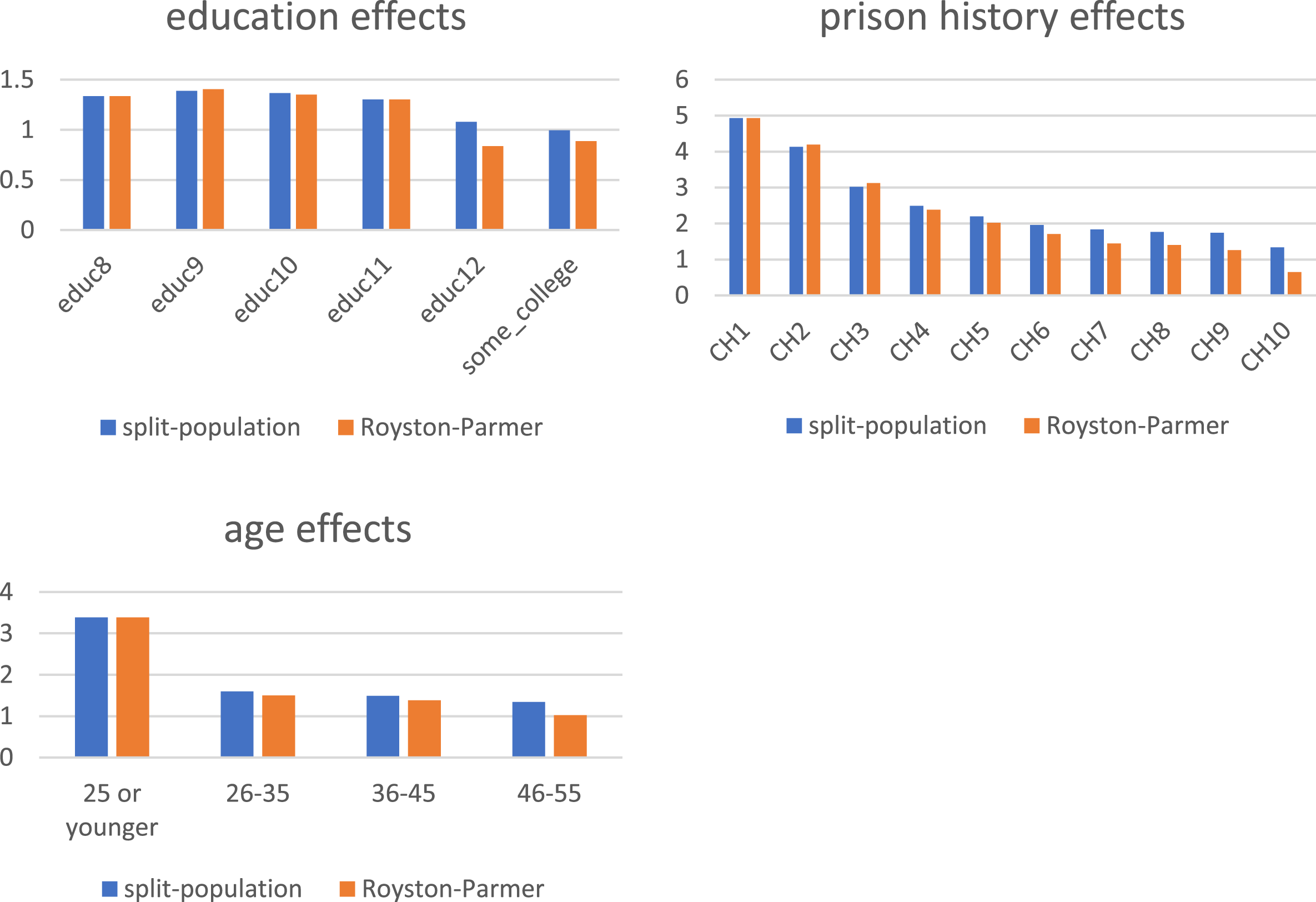

Results Regarding Correlations

We are predicting a latent variable, that is, an outcome that cannot be observed, so traditional measures of accuracy are inapplicable. To derive a measure of prediction accuracy, we use the estimated split-population model to simulate the outcome: returning to prison within three years.

How well do covariates predict the outcome: pernicious recidivism? To answer this question, we assume that supervision lasts for at least three years, and we estimate the probability of pernicious recidivism within three years based on the marginal failure distribution. We call the three-year probability a risk score. The rows of Table 3 divide predictions into five centiles (ranking). Centile 1 contains the 20% of offenders with the lowest predicted risk score, centile 2 contains the 20% of offenders with the next highest risk scores, …, and centile 5 contains the 20% of offenders with the higher risk scores. The columns differentiate estimates by the assumed value of ρ. The numbers in the table’s body are the estimated proportion of offenders who return to prison within three years of release for pernicious recidivism. These estimates are much higher than the cumulative incidence functions (Figure 6) because nuisance recidivism interrupts the occurrence of pernicious recidivism.

Table 3.

Predicted Proportion of Supervisees Returning to Prison by Prediction Ranking and ρ (0 ≤ ρ ≤ 1).

	Centiles	Assumed Values of ρ
	Centiles	1.00	.75	.50	.25	.00
Ranking	1	.20	.14	.10	.08	.06
	2	.34	.25	.19	.15	.13
	3	.47	.37	.30	.25	.20
	4	.61	.49	.41	.33	.28
	5	.72	.60	.49	.41	.34

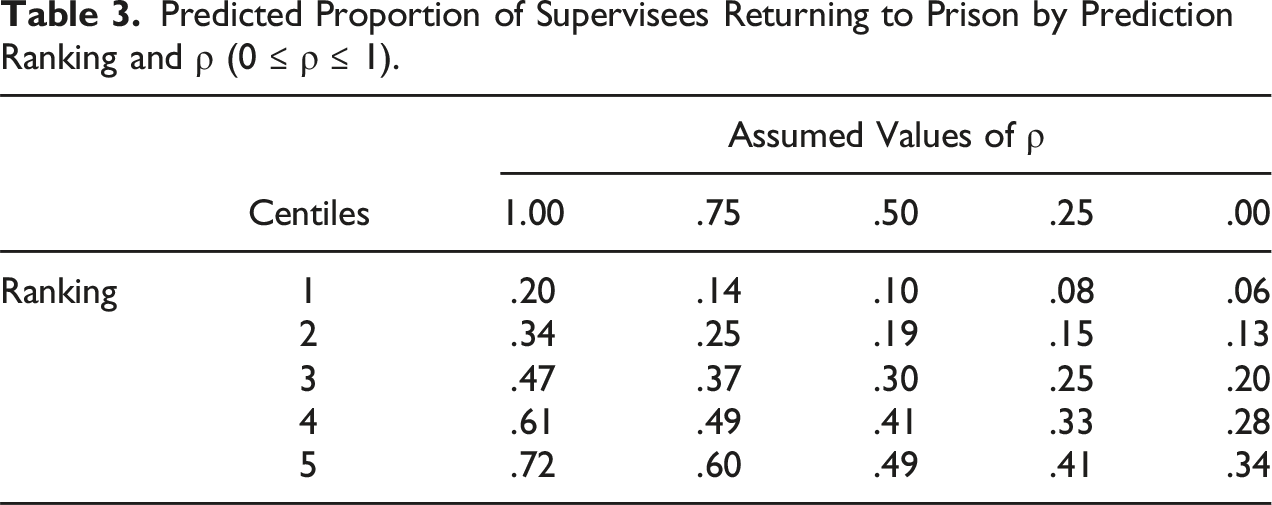
The predictions are sensitive to assumptions about ρ. The highest proportion returning to prison result from ρ = 1. The predicted proportion falls monotonically as ρ approaches 0. Most important for present purposes, we see that the model has predictive power. As the risk score ranking increases, the proportion of people returning to prison for pernicious crimes increase regardless of the value of ρ. Assuming that ρ = 1, the worst risks are 3.6 times more likely to return to prison for pernicious crime than are the best risks; assuming ρ = 0, the worst risks are 5.7 times more likely to return to prison for a pernicious crime than are the best risks. The predictors have at least a moderate ability to predict pernicious recidivism, so we turn to whether the ordering of predictions is sensitive to assumptions about ρ. In other words, as ρ varies, does the rank order of recidivism risk among people released to PCCS change or remain the same?

To perform this exercise, we set u_A and u_B to zero for every observation. We applied this constraint because, being unobserved, u_A and u_B cannot enter into predictions. First, we estimated the probability of nuisance recidivism within three years for each of five values of ρ: 1.0, .75, .50, .25, and .0. Second, we estimated the probability of pernicious recidivism within three years for the same five values of ρ. Third, using the raw data, we used a Cox model to estimate the probability of any failure within three years. Using Spearman correlation, we sought to learn the consistency of ranking offenders by risk of recidivism as ρ varies. We made four comparisons:

• We compared predictions of nuisance outcomes as ρ varied.

• We compared predictions of pernicious outcomes as ρ varied.

• We compared predictions of nuisance outcomes and pernicious outcomes for common ρ.

• We compared predictions of nuisance/pernicious outcomes with predictions of any failure based on the Cox model.

Table 4 presents the Spearman correlations for relevant comparisons. The upper left triangular matrix, shaded gray, reports the correlation across the rankings for nuisance recidivism. This is the first bulleted comparison. There exists virtually no difference in rankings regardless of the assumed value of ρ. People who are most at risk to commit a nuisance behavior are most at risk regardless of the value of ρ. People least at risk are least at risk regardless of the value of ρ. This finding might have been anticipated because alternative assumptions about ρ made little difference when predicting nuisance crimes. See Table 2.

Table 4.

Spearman Rank Order Correlations Across Predictions (ρ Between Zero and 1).

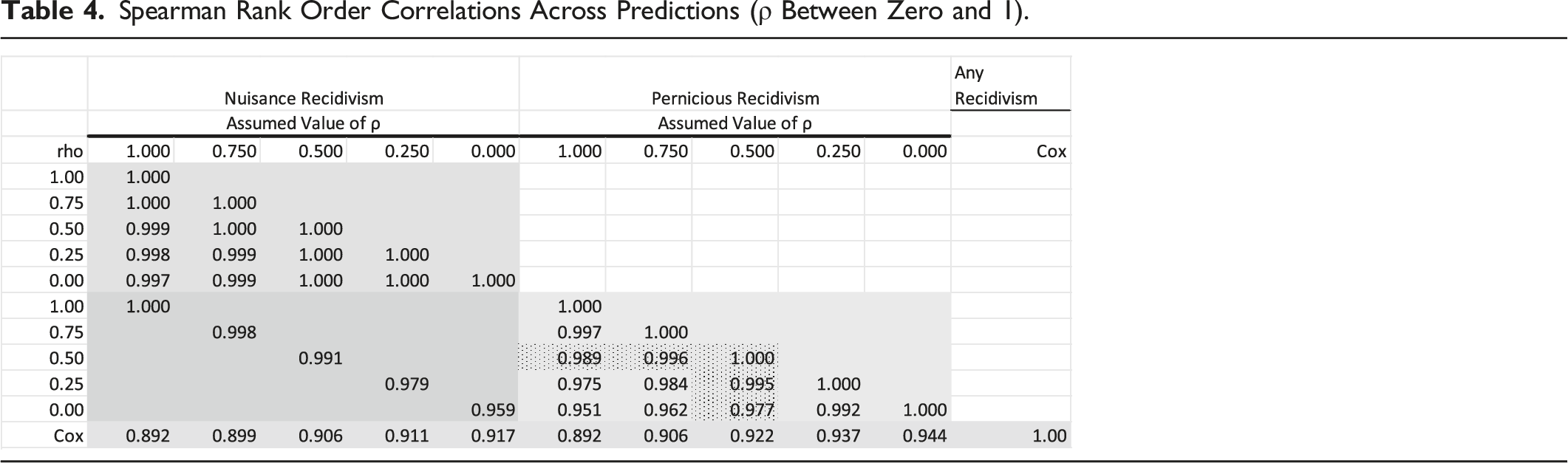
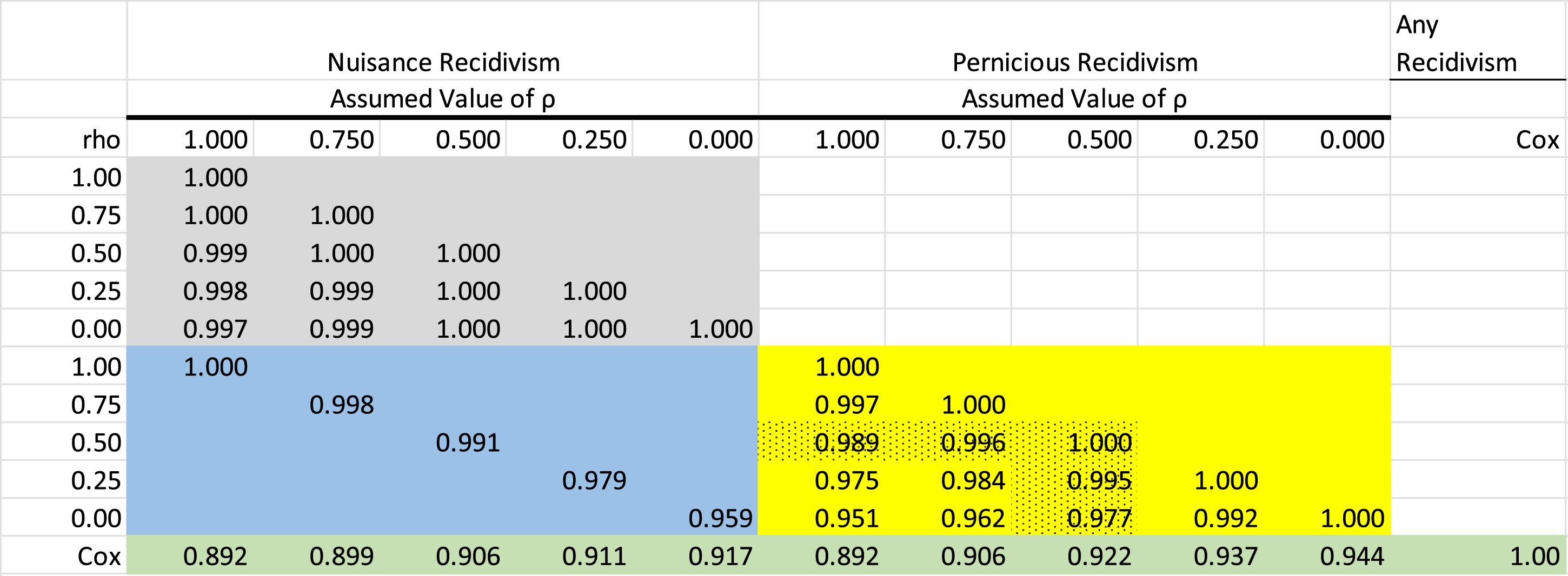
The lower right triangular matrix, shaded yellow, reports the correlation across ranking for pernicious recidivism. This is the second bulleted comparison. While predictions of pernicious recidivism vary greatly with assumptions about ρ (see Table 3), the rankings do not vary greatly with assumptions about ρ. For example, suppose we assumed ρ = .5. (See the lightly shaded yellow cells.) The resulting ranking is very similar to predictions when assuming alternative values for ρ: .989 (ρ = 1.0), .996 (ρ = .75), .995 (ρ = .25), and .977 (ρ = .0). The findings show that while different assumed values of ρ lead to different estimates of the probability of returning to prison for a pernicious recidivism, different assumed values of ρ do not lead to large differences in rankings. The rank order of the probability of committing pernicious recidivism is essentially the same regardless of the value of ρ.

The diagonal matrix, shaded blue, in the lower left corner reports the Spearman correlations for the rankings of nuisance and pernicious crimes. This is the third bulleted comparison. The matrix is diagonal because it only makes sense to compare these rankings for common values of ρ. The findings suggest little difference between offenders with a latent propensity toward nuisance recidivism and pernicious recidivism. We expand on this finding in the discussion because it has important implications for justice administration. These results show that nuisance recidivism and pernicious recidivism are highly correlated. Although this observation may come as little surprise to criminal justice researchers, a competing events survival analysis was required to provide evidence.

The bottom row, shaded green, shows the Spearman correlations between the marginal failure functions and predictions based on a Cox regression. This is the fourth bulleted comparison. The Cox regression uses any failure as its outcome criterion. Because the value of ρ is irrelevant to survival for the combined outcomes, the Spearmen correlations can be presented in a single row. The rankings based on the Cox model are consistent with the rankings based on the estimated marginal failure functions. This is further evidence of the validity of the competing risks model.

PCCS agencies often distribute rehabilitative and correctional resources after ranking FIPs into risk categories. Therefore, it is important to find that risk rankings do not vary much even when the assumed value of ρ varies considerably. If ranking risk is the purpose of a competing events model, then accuracy estimating ρ may be of less importance.³

We conducted one final set of correlations between nuisance and pernicious behaviors to answer the principal research question: What is the correlation between nuisance and pernicious recidivism? Using simulated data from the marginal distributions (including random draws of u_A and u_B), we assessed whether a FIP would experience nuisance recidivism or pernicious recidivism or both within three years. The pair of predictions were concordant when both agreed that no recidivism would occur, or both agreed that recidivism would occur. As a function of ρ, concordance was .902 (ρ = 1), .790 (ρ = .75), .713 (ρ = .50), .654 (ρ = .25), and .607 (ρ = .0). By chance, concordance would be .500 when the outcomes were independent. Although estimates at five years involve a great deal of projection, because PCCS seldom lasts so long, we can estimate concordance at five years. As a function of ρ, concordance was .946 (ρ = 1), .871 (ρ = .75), .808 (ρ = .50), .747 (ρ = .25), and .691 (ρ = .0). The answer to our principal research question depends on the value of ρ. Because the profile likelihood (Figure 5) strongly suggests a ρ between .7 and 1.0, with .9 being the best choice, we conclude that nuisance recidivism and pernicious recidivism are strongly correlated. The occurrence/nonoccurrence of one tells us much about the likely occurrence/nonoccurrence of the other.

Discussion

In support of signaling theory, we find that the latent processes leading to recidivism for nuisance behaviors and recidivism for pernicious recidivism are highly correlated. This finding suggests that revocations for nuisance behavior have utility. In a separate study (Rhodes et al., 2022), we use simulation to show that revocations for nuisance behavior can reduce both pernicious behavior (through incapacitation during a time when supervisees are at elevated risk of pernicious behavior) and prison use. The reduction in prison use may seem surprising. However, it occurs because returning a person to prison for nuisance behavior results in relatively short terms. This prevents returning to prison for pernicious behavior which, on average, imposes a long term.

We do not assert that revocation practices are optimal. Evidence-based reform is welcome. We merely observe that using revocations for nuisance behavior should not be dismissed as a correctional strategy. Revocations for nuisance behaviors can be functional.

In its recent consensus findings, the National Academy of Sciences (National Academy of Sciences, Engineering, and Medicine, 2022) broadly criticized commonly used definitions and measurements of recidivism. The Academy argued that lumping disparate outcomes (overall failure in our wording) is problematic. Not all disparate outcomes should be treated the same, because some are more harmful than others. We take this admonition seriously and have provided a principled method to distinguish failure rates for outcomes that are a nuisance from outcomes that are pernicious.

While the Academy called for considering broader measures of post-confinement behaviors such as employment and family relations, our study is limited to what is available in the NCRP. Still, even if this outcome measure is restrictive, few would argue that this measure of recidivism is unimportant for public policy.

Readers need not agree with our division of outcomes as nuisance/pernicious based on whether a revocation was caused by a new conviction. For example, an alternative measure might base the outcomes on an explicit measure of harm—nonviolent versus violent, for example. Then again, there is no requirement to dichotomize. Instead, multiple outcomes might be graded by seriousness. This is a data limitation, not a methodological limitation.⁴

The Academy also emphasized the need to recognize institutional reactions when assessing recidivism. Revoking FIPs supervision status for violations of conditions governing community supervision and for minor crimes is highly discretionary. Exercise of that discretion impacts the commission of major crime. Such reactions are central to our approach. Institutional reactions while FIPs are under community supervision distort the inherent threat posed by FIPs. Likely, risky supervisees are subjected to greater scrutiny, and risky supervisees likely have less latitude to offend before having supervision revoked. Given greater scrutiny and lesser tolerance for high-risk offenders, risk prediction for the most serious supervisees is likely distorted unless the competing event of technical revocations are considered.

One complication which we did not address is that New York State may have a set of release conditions much different from other states. Western and Harding (2022) have argued that the release context itself is criminogenic, and that by enhancing post-release resources, limiting the impact of negative labeling, and curbing the conditions of supervision, recidivism outcomes would improve. Theoretically, both the disposition of the person and these resource/environmental conditions of release both affect recidivism outcomes. They might also interact. We think this is a valid argument. There may be a substantial number of community and community supervision factors that could affect the extent to which the return for nuisance behaviors reduces the likelihood of pernicious behaviors. In seven other states, we have evaluated (Rhodes et al., 2022), we have found that prison returns for nuisance are consistently correlated with pernicious behaviors. However, there is substantial state variation in the level of this effect.

We examined only the period under post-confinement community supervision, which imposes a limitation on our analysis: We did not examine long-term outcomes that occur after supervision ends. If that seems like a limitation, it may not be a serious limitation. In a forthcoming paper, we observe that over 80% of New York State supervisees serve a single cycle of PCCS, meaning that after they are ultimately released from PCCS supervision without a revocation, they do not reenter prison. During that initial cycle, over 60% were released from PCCS without a revocation. About 30% experience a single revocation. Consequently, our analysis captures most of the outcomes generally considered to be recidivism.

Possibly, it would be worth modeling long-term recidivism. The modeling would have to recognize that revocations for nuisance behaviors could censor the occurrence of pernicious behaviors during the PCCS period but not thereafter. Such investigation goes beyond the scope of our study.

In general, criminal justice analysts who have studied recidivism have taken one of two approaches. Most have simply ignored variety in recidivism. Others who have recognized variety have either adopted a model that estimates risk for different types of recidivism without allowing one type of event to censor the other or have assumed independence. The former approach ignores censoring by a competing event and the latter makes an implausible assumption.

Our contribution is to follow National Academy recommendations to improve the study of recidivism. We have emphasized that recidivism varies regarding seriousness. Lumping all recidivism into a generic category can be misleading and is surely less informative than distinguishing levels of seriousness. We have emphasized that recidivism cannot be readily distinguished from institutional reactions. Especially, institutional reactions to nuisance recidivism have an impact on more concerning pernicious recidivism, inviting study of a correctional process that should not be dismissed offhand as dysfunctional.

Supplemental Material

Supplemental Material - Studying Parole Revocation Practices: Accounting for Dependency Between Competing Events

Supplemental Material for Studying Parole Revocation Practices: Accounting for Dependency Between Competing Events by William Rhodes, Gerald Gaes, and William Sabol in Evaluation Review.

Footnotes

Author’s Note

Georgia State University IRB number covering the work: #19082.

Declaration of Conflicting Interests

The author(s) declared no potential conflicts of interest with respect to the research, authorship, and/or publication of this article.

Funding

The author(s) disclosed receipt of the following financial support for the research, authorship, and/or publication of this article: Support for this work was provided by Arnold Ventures, Grant # 20-05227.

ORCID iDs

William Rhodes

William Sabol

Data Availability Statement

The National Corrections Reporting Program (NCRP) data used in the analyses reported in this paper are available from the National Archive of Criminal Justice Data (NACJD) at the University of Michigan’s Interuniversity Consortium on Political and Social Research (ICPSR) at . The data are from ICPSR Study Number 38491. These data are “restricted access” data that can obtained using ICPSR procedures.

Supplemental Material

Supplemental material for this article is available online.

Notes

References

Blumstein

Beck

(2005). Reentry as a transient state between liberty and recommitment. In Travis

Visher

(Eds.), Prisoner reentry and crime in America (pp. 50–79). Cambridge University Press.

Cameron

Trivedi

(2005). Microeconometrics: Methods and applications. Cambridge University Press.

Cleves

Gould

Gutierrez

Marchenko

(2010). An introduction to survival analysis using Stata (3rd ed.). Stata Press.

Coviello

Boggess

(2004). Cumulative incidence estimation in the presence of competing risks. STATA Journal: Promoting Communications on Statistics and Stata, 4(2), 103–112. https://doi.org/10.1177/1536867x0400400201

Dejong

(1997). Survival analysis and specific deterrence: Integrating theoretical and empirical models of recidivism (pp. 561–576). Criminology.

Emura

Chen

(2018). Analysis of survival data with dependent censoring: Copua-based approaches. Springer.

Gaes

Luallen

Rhodes

Edgerton

(2016). Classifying prisoner returns: A research note (pp. 48–70). Justice Research and Policy.

Gaes

G. G.

Bales

Scaggs

S. J. A.

(2016). The effect of imprisonment on recommitment: An analysis using exact, coarsened exact, and radius matching with the propensity score. Journal of Experimental Criminology, 12(1), 143–158. https://doi.org/10.1007/s11292-015-9251-x

Gendreau

Little

Goggin

(1996). Meta-analysis of the predictors of adult offender recidivism: What works. Criminolgy, 34(4), 575–607.

10.

Heckman

Honore

(1989). The identifiability of the competing risk models. Biometica, 76(2), 325–330.

11.

Heckman

Singer

(1984). The identifiability of the proportional hazard model. The Review of Economic Studies, 51(2), 231–241. https://doi.org/10.2307/2297689

12.

Kaeble

(2021). Probation and parole in the United States. Bureau of Justice Statistics.

13.

Kurlychek

Bushway

S. D.

Brame

(2012). LONG‐TERM crime desistance and recidivism patterns—evidence from the Essex county convicted felon study. Criminology, 50(1), 71–103. https://doi.org/10.1111/j.1745-9125.2011.00259.x

14.

Lambert

(2017). The estimation and modeling of cause specific cumulative incidence functions using time-dependent weights. STATA Journal: Promoting Communications on Statistics and Stata, 17(1), 181–207. https://doi.org/10.1177/1536867x1701700110

15.

Loeffler

C. E.

Nagin

D. S.

(2022). The impact of incarceration on recidivism. In Annual review of criminology (Vol. 5, pp. 133–152). Annual Reviews. https://doi.org/10.1146/annurev-criminol-030920-112506

16.

Nagin

Cullen

F. T.

Jonson

C. L.

(2009). Imprisonment and reoffending. In Tonry

(Ed.), Crime and justice: A review of research (Vol. 38, pp. 115–200). University of Chicago Press.

17.

National Academy of Sciences, Engineering, and Medicine . (2022). The limits of recidivism: Measuring success after prison. The National Academy Press.

18.

National Institute of Justice . (2021). Desistance from crime: Implications for research, policy, and practice. National Institute of Justice.

19.

Oudekerk

Kaeble

(2021). Probation and parole in the United States, 2019. Department of Justice, Bureau of Justice Statistics.

20.

Petersilia

(1997). Probation in the United States (p. 149). Crime and Justice.

21.

Piehl

A. M.

LoBuglio

S. F.

(2005). Does supervision matter? In Travis

Visher

(Eds.), Prisoner reentry and crime in America (pp. 105–138). Cambridge University Press.

22.

Reitz

Lukac

Rhine

(2020). Prison-release discretion and prison population size: State report. Robina Institute.

23.

Rhodes

Gaes

Luallen

Kling

Rich

Shively

(2014). Following incarceration, most released offenders never return to prison. Crime & Delinquency, 62(8), 1003–1025. https://doi.org/10.1177/0011128714549655

24.

Rhodes

Gaes

Sabol

(2022). The Utility of Parole Revocations: Theory and Analysis , Report prepared for Arnold Ventures.

25.

Royston

Lambert

(2011). Flexible parametric survival analysis using Stata: Beyond the Cox model. Stata Press.

26.

Royston

Parmar

M. K. B.

(2002). Flexible parametric proportional-hazards and proportional-odds models for censored survival data, with application to prognostic modelling and estimation of treatment effects. Statistics in Medicine, 21(15), 2175–2197. https://doi.org/10.1002/sim.1203

27.

Schmidt

Witte

(1988). Predicting recidivism using survival models. Springer-Verlag.

28.

Schmidt

Witte

A. D.

(1987). Predicting criminal recidivism using split population survival time models. National Bureau of Economics Research.

29.

Trivedi

Zimmer

(2005). Copula modeling: Introduction for practitioners. Now Publishers Incorporated.

30.

Tsiatis

(1975). A nonidentifiability aspect of the problem of competing risks. Proceedings of the National Academy of Sciences of the United States of America, 72(1), 20–22. https://doi.org/10.1073/pnas.72.1.20

31.

van den Berg

(2010). Competing risk models. In Durlauf

Blume

(Eds.), The new Palgrave economics collection: Microeconometrics (pp. 6–10). Palgrave McMillian.

32.

Western

Harding

(2022). Careers in criminalization: Reentry, recidivism and repeated incaceration. In Tonry

(Ed.), Crime and justice: A review of research. University of Chicago Press. https://doi.org/10.1086/721742

Supplementary Material

Please find the following supplemental material available below.

For Open Access articles published under a Creative Commons License, all supplemental material carries the same license as the article it is associated with.

For non-Open Access articles published, all supplemental material carries a non-exclusive license, and permission requests for re-use of supplemental material or any part of supplemental material shall be sent directly to the copyright owner as specified in the copyright notice associated with the article.

0.00 MB

0.68 MB