3 The survsim command
The survsim command can simulate survival data from a parametric distribution, a user-defined distribution, a fitted merlin model, a cause-specific hazards competingrisks model, or a general multistate model.
3.1 Syntax for simulating survival data from a parametric distribution
The command syntax is
survsim newvar1 [newvar2] , distribution(
string
) lambda(
numlist
) [options]
where newvar1 specifies the new variable name to contain the generated survival times. newvar2 is required when the maxtime() option is specified, which defines the times of right-censoring.
3.1.1 Options
distribution(
string
) specifies the parametric survival distribution to use, including exponential, gompertz, or weibull. All listed distributions are parameterized in the proportional hazards metric. distribution() is required.
lambda(
numlist
) defines the scale parameters in the exponential, Weibull, or Gompertz distribution. The number of values required depends on the model choice. The default is a single number corresponding with a standard parametric distribution. Under a mixture model, two values are required. lambda() is required.
gamma(
numlist
) defines the shape parameters of the Weibull or Gompertz parametric distribution. The number of entries must be equal to that of lambda(). gamma() is required for all but the exponential distribution.
noconstant suppresses the constant (intercept) term and may be specified for the fixedeffects equation and for the random-effects equations.
covariates(
varname # [varname # …] )defines baseline covariates to be included in the linear predictor of the survival model, along with the value of the corresponding coefficient. For example, a treatment variable coded 0 or 1 can be included with a log hazard-ratio of 0.5 by covariates(treat 0.5). The variable treat must be in the dataset before survsim is called.
tde(
varname # [varname # …] ) creates nonproportional hazards by interacting covariates either with log time for an exponential or a Weibull model or with time under a Gompertz model or mixture model. Values should be entered as tde(trt 0.5), for example. Multiple time-dependent effects can be specified, but they will all be interacted with the same function of time.
maxtime(
# | varname
) specifies the right-censoring times. A common maximum followup time # can be specified for all observations, or observation-specific censoring times can be specified by using a varname.
ltruncated(
# | varname
)specifies the left-truncated or delayed entry times to simulate from a conditional survival distribution. A common time can be specified for all observations by using #, or observation-specific left-truncation times can be specified by using varname.
mixturespecifies that survival times be simulated from a two-component mixture model with mixture component distributions defined by distribution(). lambda() and gamma() must be of length 2.
pmix(
#
) defines the mixture parameter. The default is pmix(0.5).
nodes(
#
) defines the number of Gauss–Legendre quadrature points used to evaluate the cumulative hazard function when mixture and tde() are specified together. To simulate survival times from such a mixture model, you use a combination of numerical integration and root finding. The default is nodes(30).
3.2 Syntax for simulating survival times from a user-defined distribution
The command syntax is
survsim newvar1 newvar2
, maxtime(
# | varname
) {loghazard(
string
) |
hazard(
string
) |
logchazard(
string
) |
chazard(
string
)} [options]
where newvar1 specifies the new variable name to contain the generated survival times and newvar2 specifies the new variable name to contain the generated event indicator.
3.2.1 Options
maxtime(
# | varname
) specifies the right-censoring times. A common maximum followup time # can be specified for all observations, or observation-specific censoring times can be specified by using a varname. maxtime() is required.
loghazard(
string
)is the user-defined log-hazard function. The user must specify one of the following: loghazard(), hazard(), logchazard(), or chazard(). The function can include the following:
{t}, which denotes the main timescale. If ltruncated() is specified, it is also measured on this timescale.
varname, which denotes a variable in your dataset.
+-*/ˆ, which are standard Mata mathematical operators, using colon notation, that is, 2:* {t}; see [M-2] op_colon. Colon operators must be used because behind the scenes, {t}gets replaced by an _N × nodes()matrix when numerically integrating the hazard function.
mata_function, which denotes any Mata function, for example, log() and exp().
hazard(
string
) is the user-defined baseline hazard function. The user must specify one of the following: loghazard(), hazard(), logchazard(), or chazard(). See loghazard() for more details and examples below.
logchazard(
string
) is the user-defined log cumulative-baseline-hazard function. The user must specify one of the following: loghazard(), hazard(), logchazard(), or chazard(). See loghazard() for more details and examples below.
chazard(
string
)is the user-defined baseline cumulative hazard function. The user must specify one of the following: loghazard(), hazard(), logchazard(), or chazard(). See loghazard() for more details and examples below.
covariates(
varname # [varname # …])defines baseline covariates to be included in the linear predictor of the survival model, along with the value of the corresponding coefficient. For example, a treatment variable coded 0 or 1 can be included with a log hazard-ratio of 0.5 by covariates(treat 0.5). The variable treat must be in the dataset before survsim is called. If chazard() or logchazard() is used, then covariates() effects are additive on the log cumulative-hazard scale.
tde(
varname # [varname # …]) creates nonproportional hazards by interacting covariates with a function of time, defined by tdefunction() on the appropriate log-hazard or log cumulative-hazard scale. Values should be entered as tde(trt 0.5), for example. Multiple time-dependent effects can be specified, but they will all be interacted with the same tdefunction(). To circumvent this, you can directly specify them in your user function.
tdefunction(
string
) defines the function of time to which covariates specified in the option tde() are interacted with to create time-dependent effects. The default is tdefunction({t}), that is, linear time. The function can include the following:
{t}, which denotes the main timescale. If ltruncated() is specified, it is also measured on this timescale.
+-*/ˆ, which are standard Mata mathematical operators, using colon notation, that is, 2:* {t}; see [M-2] op_colon. Colon operators must be used because behind the scenes, {t}gets replaced by an _N × nodes()matrix when numerically integrating the hazard function.
mata_function, which denotes any Mata function, for example, log() and exp().
ltruncated(
# | varname
) specifies the left-truncated or delayed entry times. A common time can be specified for all observations by using #, or observation-specific left-truncation times can be specified by using varname.
nodes(
#
) defines the number of Gauss–Legendre quadrature points used to evaluate the cumulative hazard function when loghazard() or hazard() is specified. To simulate survival times from such a function, you use a combination of numerical integration and root finding. The default is nodes(30).
3.3 Syntax for simulating survival times from a fitted merlin survival model
The command syntax is
survsim newvar1 newvar2
, model(
name
) maxtime(
# | varname
)
where newvar1 specifies the new variable name to contain the generated survival times and newvar2 specifies the new variable name to contain the generated event indicator.
3.3.1 Options
model(
name
) specifies the name of the estimates store object containing the estimates of the fitted model. The survival model must be fit using the merlin command. survsim will simulate from the fitted model, using covariate values that are in your current dataset. model() is required. For example,
merlin (_t trt, family(weibull, failure(_d)))estimates store m1
survsim stime died, model(m1) maxtime(10)
maxtime(
# | varname
) specifies the right-censoring times. A common maximum followup time # can be specified for all observations, or observation-specific censoring times can be specified by using a varname. maxtime() is required.
3.4 Syntax for simulating survival times from a multistate model
The command syntax is
survsim
timestub statestub eventstub
, hazard1(
haz_options
)
hazard2(
haz_options
) maxtime(
# | varname
) transmatrix(
name
)
hazard3(
haz_options
) options]
where timestub specifies the new variable name stub to contain the generated survival times for each transition. statestub specifies the new variable name stub to contain the generated state identifiers, that is, which state each observation has transitioned to or is in, at the associated times. eventstub specifies the new variable name stub to contain the event indicators, that is, whether an event or right-censoring occurred at the associated times. When observations have reached an absorbing state or reached maxtime(), they will have missing observations in any further generated variables. When all observations have reached an absorbing state or are right-censored, then the simulation will cease, and the generated variables are returned.
Each hazard
#
(
haz_options
) represents a transition-specific hazard function, where # is used to index the transition in the transition matrix, defined in transmatrix().
3.4.1 Options
hazard
#
(
haz_options
) represents a transition-specific hazard function, where # is used to index the transition in the transition matrix, defined in transmatrix(). hazard1() and hazard2() are required. haz_options are the following:
distribution(
string
)specifies the parametric survival distribution to use, including exponential, gompertz, or weibull. All listed distributions are parameterized in the proportional hazards metric. Either distribution() or user() must be specified.
lambda(
#
) defines the scale parameter for an exponential, Weibull, or Gompertz distribution. lambda() is required.
gamma(
#
) defines the shape parameter for a Weibull or Gompertz parametric distribution. gamma() is required for all but the exponential distribution.
user(
function
)defines a custom hazard function. Either user()or distribution() must be specified. The function can include the following:
{t}, which denotes the main timescale. If ltruncated() is specified, it is also measured on this timescale.
{t0}, which denotes the time of entry to the current state of the associated transition hazard, measured on the time since initial starting state timescale.
varname, which denotes a variable in your dataset.
+-*/ˆ, which are standard Mata mathematical operators, using colon notation, that is, 2:* {t}; see [M-2] op_colon. Colon operators must be used because behind the scenes, {t} gets replaced by an _N × nodes()matrix when numerically integrating the transition hazard function.
mata_function, which denotes any Mata function, for example, log() and exp().
For example,
distribution(weibull) lambda(0.1) gamma(1.2) is equivalent to
user(0.1:*1.2:*{t}:ˆ(1.2:-1))
covariates(
varname # [varname # …]) defines baseline covariates to be included in the linear predictor of the transition-specific hazard function, along with the value of the corresponding coefficient. For example, a treatment variable coded 0 or 1 can be included with a log hazard-ratio of 0.5 by covariates(treat 0.5). The variable treat must be in the dataset before survsim is called.
tde(
varname # [varname # …] ) creates nonproportional hazards by interacting covariates with a function of time. Covariates are interacted with the specification in tdefunction() on the log-hazard scale. Values should be entered as tde(trt 0.5), for example. Multiple time-dependent effects can be specified, but they will all be interacted with the same function of time.
tdefunction(
string
) defines the function of time to which covariates specified in the option tde() are interacted with to create time-dependent effects in the transition-specific hazard function. The default is tdefunction({t}), that is, linear time. The function can include the following:
{t}, which denotes the main timescale. If ltruncated() is specified, it is also measured on this timescale.
+-*/ˆ, which are standard Mata mathematical operators, using colon notation, that is, 2:* {t}; see [M-2] op_colon. Colon operators must be used because behind the scenes, {t} gets replaced by an _N × nodes()matrix when numerically integrating the transition hazard function.
mata_function, which denotes any Mata function, for example, log() and exp().
reset specifies that this transition model be on a clock-reset timescale. The timescale is reset to 0 on entry; that is, the timescale for this transition is measured on a time since state entry timescale rather than the default clock-forward. If you specify a user() function with reset, then survsim will replace any occurrences of {t} with {t}-{t0}, including those specified in tdefunction().
maxtime(
# | varname
) specifies right-censoring times. A common maximum follow-up time # can be specified for all observations, or observation-specific censoring times can be specified by using a varname. maxtime() is required.
transmatrix(
matname
) specifies the transition matrix that governs the multistate model. Transitions must be numbered as an increasing sequence of integers from 1,…, K, from left to right, top to bottom of the matrix. Reversible transitions are allowed. By default, a competing-risks model is assumed.
startstate(
# | varname
) specifies the states in which observations begin. A common state # can be specified for all observations, or observation-specific starting states can be specified by using a varname. The default is startstate(1).
ltruncated(
# | varname
) specifies left-truncated or delayed entry times, which are the times at which observations start in the initial starting states. A common time can be specified for all observations by using #, or observation-specific left-truncation times can be specified by using varname. The default is ltruncated(0).
nodes(
#
) defines the number of Gauss–Legendre quadrature points used to evaluate the total cumulative hazard function for each potential next transition. To simulate survival times from such a function, you use a combination of numerical integration and root finding. The default is nodes(30).
4 Examples
In this section, I will go through at least one example of how to use survsim to simulate survival data from each of the four main settings.
4.1 Simulating survival times from standard parametric distributions
Let’s simulate survival times from a Weibull distribution with a binary treatment group, trt, and a continuous covariate, age, under proportional hazards

I will simulate 300 observations and pick some distributions for the covariates, which should be self-explanatory:

We then call survsim, setting λ = 0.1, γ = 1.2, β
1 = −0.5, and β
2 = 0.01,
. survsim stime, distribution(weibull) lambda(0.1) gamma(1.2)
> covariates(trt -0.5 age 0.01)
which stores our simulated survival times in the new variable stime. If we wanted to apply right-censoring, we could first generate some censoring times. We could apply a common censoring time using, for example, maxtime(5), which would censor all observations if their simulated event times were greater than 5, or we could generate observation-specific potential censoring times such as
. generate censtime = runiform() * 5
Now we add the maxtime() option to survsim, remembering to also specify a second new variable name for the event indicator:
. survsim stime2 died2, distribution(weibull) lambda(0.1) gamma(1.2)
> covariates(trt -0.5 age 0.01) maxtime(censtime)
We could also
add time-dependent effects using the tde() option,
add left-truncation or delayed entry using the ltruncated() option, or
simulate from a two-component mixture distribution using the mixture option.
4.2 Simulating survival times from a user-defined (log) (cumulative) hazard function
This section illustrates how to simulate from a user-defined function, first described in Crowther and Lambert (2013). Let’s start by simulating 500 observations and generate a binary treatment group:

The most flexible form of simulating survival data with survsim is by specifying a custom hazard or cumulative hazard function, such as

where

which can be done on the loghazard() scale for simplicity, using

The loghazard() function is defined using Mata code with colon operators representing element-by-element operations. Time must be referred to using the {t}notation. A common right-censoring time of 1.5 years is specified using maxtime(1.5). We could make the treatment effect diminish over log time by incorporating a time-dependent effect, where
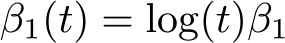
which is defined using the tdefunction() and tde() options, setting β
1 = 0.03:

This will form an interaction between trt, its coefficient 0.03, and log time. Alternatively, we could instead simulate from a model on the cumulative hazard scale, using the logchazard() option instead.
4.3 Simulating survival times from a fitted merlin survival model
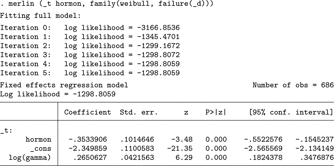
Rather than simulating from a particular data-generating model specified essentially by hand, we can directly simulate from a fitted model by passing an estimates object to survsim through the model() option. This is similar to stsurvsim (Royston 2012), which allows the simulation of survival times from a Royston–Parmar flexible parametric model. survsim now allows simulation from a survival model that has been fit with the merlin command. Let’s fit a Weibull model to a standard survival dataset:


I am using the benefits of stset to declare the survival variables, which I can use directly within merlin for simplicity. We then simply store the model object, calling it whatever we like, such as the imaginative name of m1:
. estimates store m1
We then pass this to survsim to simulate a dataset of the same size using our fitted results:
. survsim stime5 died5, model(m1) maxtime(7)
The option maxtime() is required in this case. We can then fit the same model as before, and of course get slightly different results, because we have sampling variability:

Note that survsim will simulate the same number of observations as _N, so any covariates in your model must have nonmissing observations; otherwise, missing values will be produced. The useful aspect of this is that you can manipulate your covariate distributions in your dataset and then simply recall survsim to simulate new survival times using the same estimated parameters.
Currently, survsim can simulate from any of the available survival models in merlin but does not support simulation from multivariate models or a model containing random effects.
4.4 Simulating competing-risks data from specified cause-specific hazard functions

Each specification of hazard
#
() defines a cause-specific hazard function with the specified distribution() and associated baseline parameters, covariate effects, and time-dependent effects. Each of the hazard
#
() functions can be as similar or as different as required. survsim creates some new variables based on the newvarstubs that we specified in the call.

Because the competing-risks simulation is framed within a more general multistate setting, discussed in the next example, all observations are assumed to begin in an initial starting state 1 and an initial starting time 0. These are stored in state0 and time0, respectively. The starting time can be changed using the ltruncated() option.
From the starting state, observations have two places to go:
State 1 to State 2 with the transition rate governed by hazard1().
State 1 to State 3 with the transition rate governed by hazard2().
We can see which events occurred with

which shows that by 10 years, 484 observations were right-censored, 414 are in state 2, and 102 are in state 3.
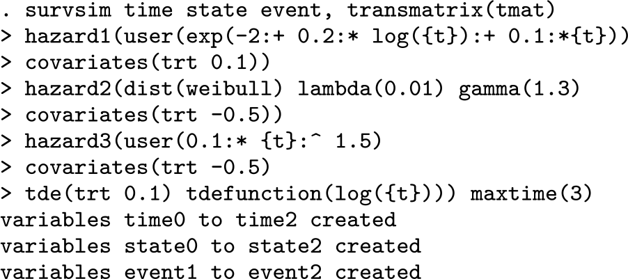
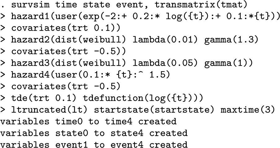
Now let’s simulate from a competing-risks model with three competing events. The first cause-specific hazard has a user-defined baseline hazard function with a harmful treatment effect. The second cause-specific hazard model has a Weibull distribution with a beneficial treatment effect. The third cause-specific hazard has a user-defined baseline hazard function with an initially beneficial treatment effect that reduces linearly with respect to log time. Right-censoring is applied at three years.

You can see that this can get as complex as necessary. I currently let you use up to 50 cause-specific hazards, just in case you are feeling particularly adventurous.
4.5 Simulating from an illness-death model
We first define the transition matrix for an illness-death model. It has three states:
State 1: A healthy state. Observations can move from state 1 to state 2 or state 3.
State 2: An intermediate ill state. Observations can come from state 1 and move on to state 3.
State 3: An absorbing dead state. Observations can come from state 1 or state 2 but not leave.
This gives us three potential transitions between states:
Transition 1: State 1 → State 2
Transition 2: State 1 → State 3
Transition 3: State 2 → State 3
This is defined by the following matrix:
. matrix tmat = (.,1,2\.,.,3\.,.,.)
The key is to think of the column or row numbers as the states and the elements of the matrix as the transition numbers. Any transitions indexed with a missing value (.) means that the transition between the row state and the column state is not possible. Let’s make it obvious, sticking with our healthy, ill, and dead names for the states:

Now that we have defined the transition matrix, we can use survsim to simulate some data. We will simulate 1,000 observations and generate a binary treatment group indicator, remembering to set seed first.

The first transition-specific hazard has a user-defined baseline hazard function with a harmful treatment effect. The second transition-specific hazard model has a Weibull distribution with a beneficial treatment effect. The third transition-specific hazard has a user-defined baseline hazard function with an initially beneficial treatment effect that reduces linearly with respect to log time. Right-censoring is applied at three years.
The hazard number # in each hazard
#
() represents the transition number in the transition matrix. Simple as that. survsim has created variables storing the times at which states were entered with the associated state number and the associated event indicator. It begins by creating the 0 variables, which represent the time at which observations entered the initial state, time0, and the associated state number, state0. Because ltruncated() and startstate() were not specified, all observations are assumed to start in state 1 at time 0. Subsequent transitions are simulated until all observations either have entered an absorbing state or are right-censored at their maxtime(). For simplicity, I will assume time is measured in years. We can see what survsim has created:

All observations start initially in state 1 at time 0, which are stored in state0 and time0, respectively. Then the following happens:
Observation 1 is right-censored at 3 years, remaining in state 1.
Observation 4 moves to state 2 at 0.956 years and is subsequently right-censored at 3 years, still in state 2.
Observation 16 moves to state 2 at 1.076 years and then moves to state 3 at 2.440 years. Because state 3 is an absorbing state, there are no further transitions.
Observation 112 moves to state 3 at 2.329 years. Again, because state 3 is absorbing, there are no further transitions.
We could incorporate a variety of extensions; for example, we could simulate from a semi-Markov model by using the reset option in hazard3(), which would reset the clock when state 2 is entered. The simulated event times that survsim returns will still be calculated on the main timescale in this case, time since initial startstate(). We could have, of course, a much more complex multistate structure, that is, more states or reversible transitions. Both of these are supported by survsim.
4.6 Simulating from an illness-death model with multiple timescales
A further capability of survsim is to simulate from an event-time model with multiple timescales. Such a setting is rarely considered because the estimation of such a model is computationally challenging, let alone simulating from one. However, survsim now provides this in an extremely general way, and indeed merlin can fit such models.
Continuing with the illness-death model, the transition between the illness and death state may depend not only on time since the initial healthy state entry but also on the time since illness. More formally, we can define the transition rate for state 2 to state 3 as

where h
30(t) is the baseline hazard function on the main timescale, time since entry to the healthy state 1. We have a vector of baseline covariates with associated log hazardratios, X and β
31, respectively. Finally, we define t
30 to be the time at which the observation entered state 2, and hence (t − t
30) defines the time since entry to state 2. Our function f() can be as simple or complex as required with associated coefficient vector β
32.
For simplicity, I will assume a linear effect of time since entry to state 2, incorporating it into the illness-death transition models from the previous section, setting β
32 = −0.05, meaning a longer time to illness reduces the mortality rate.

To refer to the entry time for a particular transition, we use {t0} alongside our usual {t} denoting time since study origin, and hence ({t}:-{t0}) allows us to define time since state entry. Of course, this can be extended in numerous ways.
4.7 Simulating from a reversible illness-death model
I now extend the example from section 4.5 to allow for recovery; that is, observations can move from the ill state back to the healthy state. Our transition matrix now looks like this:

Remember, transitions must be indexed going from top left to bottom right, along columns, and then down rows. So transition 3 is our new transition, going from ill to healthy.
Once again, we will simulate 1,000 observations and generate a binary treatmentgroup indicator, remembering to set seed first. However, now I will add delayed entry, allowing each observation to enter the study at a time greater than 0. Remember, entry and transition times are all simulated and recorded on the main overall timescale, even if the clock is reset on state entry. I will also vary the starting state of the observations, allowing observations to enter in either state 1 or state 2.

The first transition-specific hazard has a user-defined baseline hazard function with a harmful treatment effect. The second transition-specific hazard model has a Weibull distribution with a beneficial treatment effect. The third transition has a Weibull distribution with no covariate effects. The fourth transition-specific hazard has a user-defined baseline hazard function with an initially beneficial treatment effect that reduces linearly with respect to log time. Right-censoring is applied at three years.
Because ltruncated() and startstate() were specified, observations start in different states and at different times. Subsequent transitions are simulated until all observations either have entered an absorbing state or are right-censored at their maxtime(). For simplicity, I will assume time is measured in years. We can see what survsim has created:

Starting state and times are stored in state0 and time0, respectively. We see the following:
Observation 1 enters state 1 at 0.0026 years and remains there until being rightcensored at three years.
Observation 695 enters state 2 at 0.7018 years, recovers to state 1 at 1.244 years, has a relapse at 1.920 years, moving to state 2, recovers again at 2.259 years, and remains there until the end of follow-up.
Observation 704 enters state 2 at 1.279 years, recovers to state 1 at 2.386 years, has a relapse at 2.464 years, moving to state 2, and subsequently dies at 2.9616 years, moving to state 3.
Note that in this case, we had four sets of new variables created. If we extend follow-up, then we will obtain more because we have a reversible process and survsim will simply continue to simulate transitions for observations until all observations have reached an absorbing state or the maximum follow-up time.