Deep Learning–Based Detection of Endothelial Tip Cells in the Oxygen-Induced Retinopathy Model

Abstract

Proliferative retinopathies, such as diabetic retinopathy and retinopathy of prematurity, are leading causes of vision impairment. A common feature is a loss of retinal capillary vessels resulting in hypoxia and neuronal damage. The oxygen-induced retinopathy model is widely used to study revascularization of an ischemic area in the mouse retina. The presence of endothelial tip cells indicates vascular recovery; however, their quantification relies on manual counting in microscopy images of retinal flat mount preparations. Recent advances in deep neural networks (DNNs) allow the automation of such tasks. We demonstrate a workflow for detection of tip cells in retinal images using the DNN-based Single Shot Detector (SSD). The SSD was designed for detection of objects in natural images. We adapt the SSD architecture and training procedure to the tip cell detection task and retrain the DNN using labeled tip cells in images of fluorescently stained retina flat mounts. Transferring knowledge from the pretrained DNN and extensive data augmentation reduced the amount of required labeled data. Our system shows a performance comparable to the human level, while providing highly consistent results. Therefore, such a system can automate counting of tip cells, a readout frequently used in retinopathy research, thereby reducing routine work for biomedical experts.

Introduction

Proliferative retinopathies, such as diabetic retinopathy (DR) and retinopathy of prematurity, are the leading causes of vision impairment and blindness in working-age adults and children in developed countries. ¹ An early event in the development of proliferative retinopathies is the degeneration of the retinal microvasculature, followed by ischemia. ² The ischemia induces the recruitment of new blood vessels to the malperfused retina. However, instead of a revascularization of the ischemic areas in the retina, a misbalance of growth and guidance factors causes an aberrant angiogenesis with so-called neovascular tufts protruding into the vitreous. ³ These neovessels are nonfunctional and can cause complications such as traction on the retina and retinal bleeding. In addition, the overproduction of specific growth factors can trigger the formation of edema.

Current treatment options focus on the late vascular changes in proliferative retinopathies and edema. Treatments include laser photocoagulation and injections of vascular endothelial growth factor inhibitors (anti-VEGF) or corticosteroids. ^4,5 These therapies can improve vision and reduce the risk of vision loss for many patients. Nevertheless, a significant number of patients do not fully respond to the existing treatments. ⁶ Exploring novel therapeutic options is therefore required to overcome the limitations of the current standard of care. This is of particular importance in light of the large prevalence and the potential severe consequences such as blindness.

A frequently employed animal model for studying compound effects on ischemia-driven proliferative retinopathies is the oxygen-induced retinopathy (OIR) model in the mouse. ^7,8 Neonatal mice are exposed to 75% oxygen from postnatal day 7 to 12, thereafter the animals return to room air (21% oxygen) until day 17. At day 7, the mouse retinal vasculature is still in a developmental phase and vulnerable to the high oxygen conditions. Regression of the immature capillaries in the center of the retina leads to the formation of an avascular area (see Figure 1). Upon return to room air at day 12, the area becomes hypoxic and angiogenic growth is triggered. Dysregulated angiogenesis in this model can lead to neovascularization with histological features such as neovascular tufts that resemble those noted in patients with proliferative retinopathies. On the other hand, the ischemic retina can be revascularized by healthy retinal vessels over time. ^9,10 Thus, the OIR model offers readouts that are useful for distinguishing between physiological and pathophysiological angiogenesis and is popular to study compound effects on vascular guidance.

Figure 1.

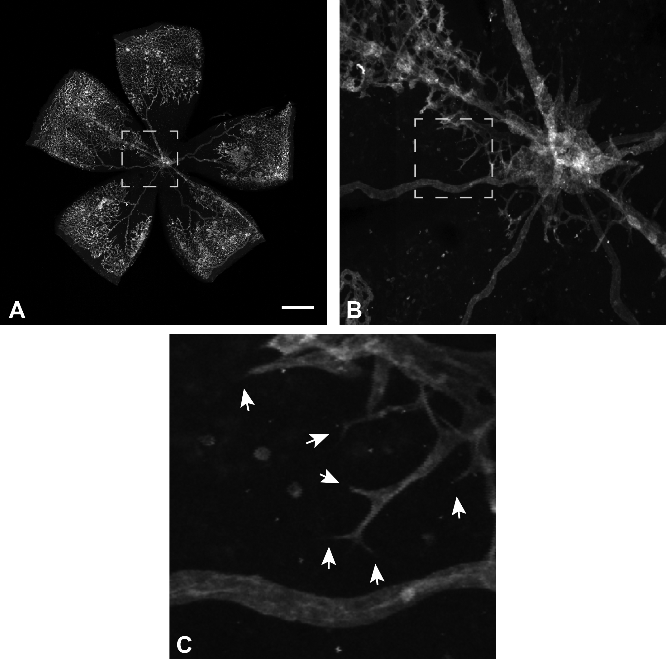
Confocal microscopy image of a mouse retina flat mount at different magnification levels. The retina vasculature was labeled with fluorescently tagged isolectin. In the overview A and the magnified center B an avascular area is visible in the center (formed by the oxygen-induced retinopathy [OIR] model). The highest magnified region C shows several spouting tip cells (see arrows) growing into the avascular area. Scale bar: 500 µm.

Flat mount preparations of the retina stained with fluorescently tagged isolectin, which labels the vasculature (Figure 1), are widely used for analysis of the efficacy of compounds designed to prevent neovessel formation and to increase vascular repair. Image analysis allows the analysis of the vasculature in flat mounts. For example, area quantification of prominent vascular abnormalities (such as the avascular area or neovascular tuft area) can be done automatically. ^9,11

Quantitation of tip cells (Figure 1) at the avascular front is a particularly promising readout in the OIR model to assess revascularization of ischemic regions. Tip cells are specialized endothelial cells located at the tips of vascular sprouts that extend long filopodia. These dedicated morphological features enable to sense growth factor gradients in order to guide newly forming vessels. Tip cells therefore directly indicate new vessel sprouting. ^12,13 Tip cells can be visually identified based on their morphology and location. Usually they are oriented to the direction of avascular area and have pointed ends. Until now, tip cell counting has relied on manual cell identification by a trained expert, which is a tedious task and is subject to nonavoidable inter- and intraobserver variability. With the emergence of deep learning (DL)–based computer vision approaches, it is now possible to automate this task.

Deep learning is a branch of machine learning that coarsely mimics a network of biological neurons with artificial neurons as basic computational units. Such networks use at least a few layers of artificial neurons, hence the name. The strength of connection between a pair of neurons in adjacent layers is encoded with parameters, called weights. In order to set deep neural network (DNN) optimal parameters, DNNs are usually trained on a large number of examples. When a large number of labeled examples is not available for the task at hand, a DNN can be trained on a related task with a large number of labeled examples followed by the second stage of training on the original task (fine-tuning) with a smaller number of examples. In this way, the knowledge obtained from the related task and stored in the DNN’s parameters is transferred to the original task, which is referred to as transfer learning.

With the recent advances of the field of DL, ¹⁴ many complex tasks such as image or speech recognition are now feasible for computers. A specific DNN architecture, Convolutional Neural Networks ^15,16 (CNNs), is particularly successful in computer vision tasks such as image classification (assigning images to predefined categories), object detection (finding bounding boxes around all detected objects and assigning them to categories), and segmentation (assigning all the pixels to categories). Given sufficient amount of labeled data (images, objects, or pixels according to the task), these tasks can be automated yielding results at human or even superior to human performance levels, which previously was only possible for restricted problems under controlled conditions. These approaches already have had a great success in various branches of medical image analysis, ¹⁷ such as histology ^{18 -21} or ophthalmology. ²² Moreover, an artificial intelligence–based diagnostic system for detection of DR without any human supervision has been recently approved by the US Food and Drug Administration. ²³

Here, we demonstrate a DL-based approach for automation of the task of tip cell counting in retina flat mounts. Our approach achieves human-level performance and allows the fully automated analysis of flat mounts. This not only reduces the routine work for biomedical experts but also yields more consistent tip cell readouts, which is important for retinopathy research.

Material and Methods

Annotated Data Set of Retina Flat Mount Images

Oxygen-induced retinopathy retina flat mount images

Pregnant C57BL/6J mice with a specified mating data were obtained from Charles River. The day of birth is defined as postnatal day 0 (P0). Experimental protocols concerning the use of laboratory animals were reviewed by a Federal Ethics Committee and approved by governmental authorities. At P7, mouse pups were put into chambers in which the oxygen content was increased to 75%. Animals remained in the high oxygen atmosphere for 5 days and returned to room air at P12. At P15 or P17, animals were killed by cervical dislocation under isoflurane anesthesia and eyes were enucleated.

Eyes were fixed in paraformaldehyde (4%) for 1 hour at 4 °C and were then transferred to phosphate-buffered saline (PBS) and retinae were isolated. Retinae were incubated overnight at 4 °C with 1% BSA, 0.5% Triton X-100 in PBS and washed with 1 mM CaCl₂, 1 mM MgCl₂, and 0.1 mM MnCl₂ in PBS. Staining was performed in the same buffer containing 0.02 mg/mL fluorescein isothiocyanate (FITC) labeled isolectin B4 overnight at 4 °C in the dark. Retinae were then washed with PBS, postfixed for 5 minutes with PFA and washed again. Each retina was transferred to a glass slide and cut approximately 4 times to achieve a flat cloverleaf-like structure. The tissue was covered with mounting medium and a coverslip was put on top to obtain a retinal flat mount.

Images of the retinal flat mounts were acquired by exciting the samples with a wavelength of 488 nm using a laser scanning microscope (LSM) 700 confocal laser scanning-microscope (Carl Zeiss) with a 10× objective at a resolution of 1.25 μm/pixel (see an example in Figure 1). In order to confirm the robustness of the system to different acquisition systems, in the section Comparison of Tip cell Counts, we did experiments with images acquired with the Opera Phenix high-content screening (HCS) system (PerkinElmer) using comparable imaging parameters, in particular a pixel resolution of 1.25 µm/pixel. No new animal studies were carried out specifically for our project, only historical archived data were used.

Data sets

We prepared a data set of 220 retina flat mount images with labeled tip cells for training of the tip cell detector. All images were from either different mice or different eyes of the same mouse (140 mice with flat mount images from only one eye and 40 mice with flat mount images from both eyes). A skilled person (N.Z.) manually labeled 17,994 tip cells in these images. N.Z. is a biomedical scientist with years-long experience in the field of angiogenesis. Additionally, 2 smaller validation and test data sets were built, consisting of 16 and 25 annotated flat mount images, correspondingly. The validation data set was used to tune parameters related to the training process and the system architecture. The separated test data set was used for the estimation of the final system performance. All the images are gray-scale images of 5120 × 5120 pixel size (see an example in Figure 1). There was no overlap between mice used for test and train (or validation) data sets. Since our detector is designed to work with images of 512 × 512 size, the images, before being processed, are tiled to patches of this size. Correspondingly, the coordinates of labeled tip cells were updated to match the created patches. For training, we generated patches with a small overlap of 12.5% to avoid loss of labeled tip cells located at patch borders.

The labeling work was done with the use of the Zeiss Efficient Navigation (ZEN) software (Carl Zeiss). Zeiss Efficient Navigation is an image acquisition, processing, and analysis software for digital microscopy developed by Zeiss. The software allows image manipulation and annotation of image regions with various graphical tools. In our case, tip cell locations (tip cell ends) were labeled with point markers (see Figure 2, top-left). We designed a software that collects the labels saved by ZEN in xml files and feeds them to our training pipeline. In most cases, tip cells are directed into the direction of avascular area, have pointed ends due to filopodial extensions, and are located at tips of vessel sprouts. The typical range of the tip cell sizes is between 25 and 60 µm, though usually we do not see the whole 3-dimensional cell in the 2D images.

Figure 2.

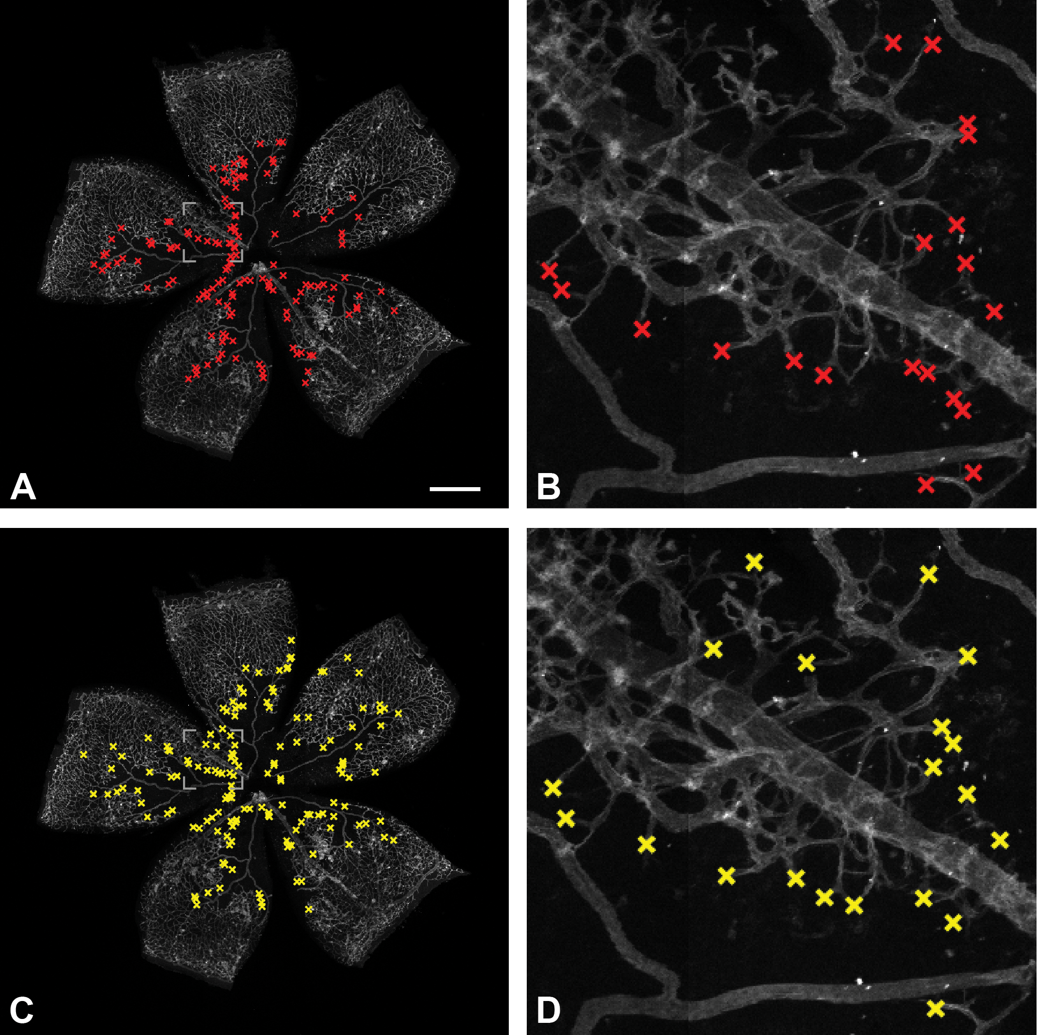
An example of a retina flat mount image with tip cells labeled by the reference expert (A, B) and automatically detected by the system (C, D). Magnified regions of ground truth labels and detections are shown on the right. Scale bar: 500 µm.

Flat mount masks

We use binary masks of flat mount areas in order to exclude background regions (black in Figure 3) from being used in a few stages of the detection pipeline (sections Redesigned SSD: DNN Model, Hard Negative Mining, Post-processing). To generate flat mount masks, images were first smoothed by an edge-preserving smoothing algorithm ²⁴ and scaled down to 25% of the original size. The region growing algorithm was applied after image gray values were converted to the [0-255] range. The region growing started from 8 points taken from the vicinity of the image corners. At any point in the process of the region growing, the mean gray value of the current region is calculated. New pixels were added to the region if they differ from the current region mean by less than 3 gray levels. The complement of the generated image was further smoothed with morphological closing, which also eliminated small holes. The resulting image mask was scaled back to the original image size.

Figure 3.

Retina flat mount mask of the image in Figure 1.

Redesigned Single-Shot-Detector (SSD)

Application of DNNs to the object detection task has shown remarkable advances in the last years. ^25,26 The first DNN detectors were based on patch image classifiers. Later, they evolved to more computationally effective detectors with dedicated architectures. Such DL-based detectors outperform all the other types of detectors with a large margin when evaluated on large data sets of natural images.

There are 2 types, one and two stage, DNN object detectors. The two-stage object detectors include a fast object proposal unit as a first stage, where an object of any type is first detected. It is then categorized at the second, more computationally demanding object classification stage. Since in our case we detect only a single type of objects, tip cells versus a vascular background, we use an one-stage object detector, where the object of interest is directly detected.

Redesigned SSD: DNN Model

We have chosen one of the successful (state-of-the-art 2016) one-stage DNN object detectors, the SSD. ²⁷ The SSD has a relatively simple architecture that generalizes fairly well on different types of images, which over a few recent years allowed its extensive use in a broad range of applications. It is one of the fast detectors and has a few open-source high-quality implementations available online, upon one of which we built our system. ²⁸ Based on the principles of transfer learning, the SSD uses a truncated VGG-16 network ²⁹ pretrained on the ImageNet data set. ³⁰ In the SSD, the fully connected VGG layers were converted to convolutional layers and extra convolutional layers were added to generate several multiscale feature maps.

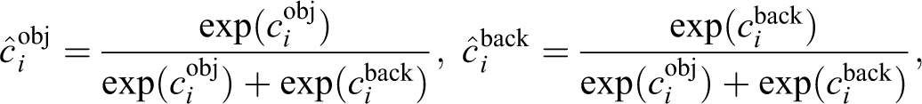
Our task is more restricted than generic object detection. We can therefore refine the original SSD architecture, thereby reducing the number of parameters to be learned. The refined SSD-512 architecture is shown in Figure 4. We experimented with the number of multiscale feature maps and concluded that for our task layers on the top of the truncated VGG base network do not improve the performance of our system. This is explained by the fact that the structures of interest are of approximately similar size, which is relatively small. Detection of objects of such size requires the use of the feature map at highest resolution. We therefore use only a single-scale feature map of 64 × 64 spatial size and exclude both SSDs extra convolutional layers and VGGs fully connected layers, which were converted to convolutional layers in the original SSD architecture. We also use only a single square default bounding box (64 pixels size), which matches the size of bounding boxes around labeled tip cells. Thus, for each location in a 64 × 64 feature map, the detector computes a pair of confidence score values c^obj, c^back and a pair of positional offset l^cx, l^cy values (see Equation 3). After a softmax operation, the resulting object’s confidence value ${\widehat{c}}^{obj}$ is thresholded at a suitable level to determine whether an object is present at the corresponding offset location in the input image.

Figure 4.

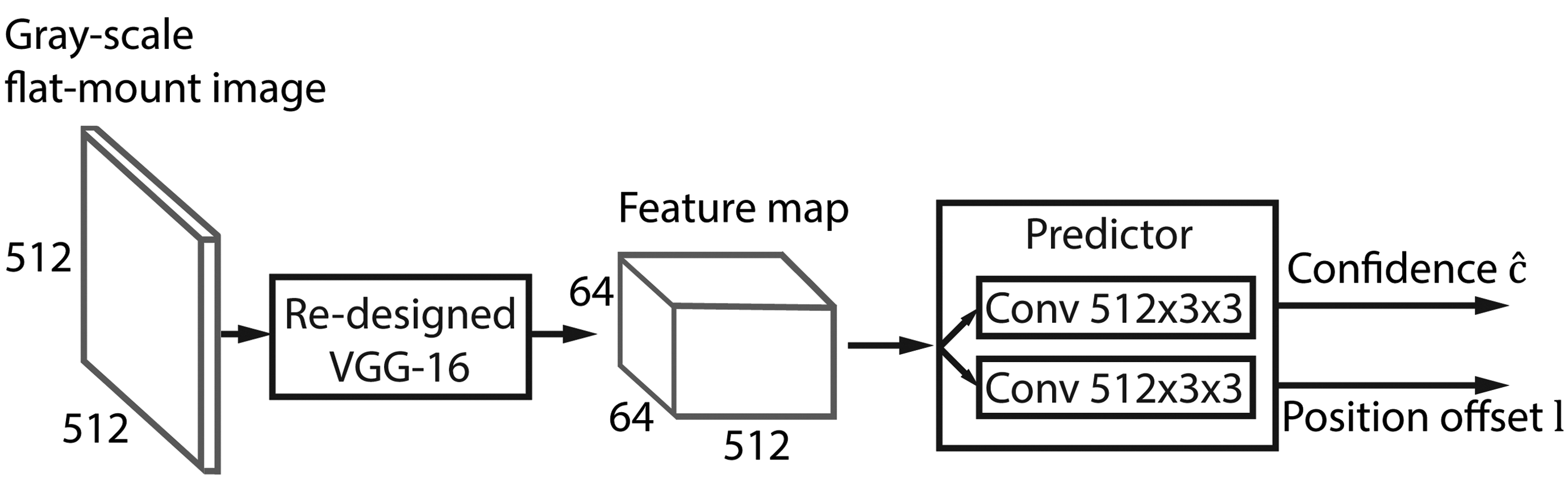
Refined Single Shot Detector (SSD) architecture consists of a modified VGG-16 backbone that generates a feature map at a single resolution and a predictor of confidence and position offset for each of 64 × 64 spatial locations. VGGs first layer filters are shrunk to 1 × 3 × 3 size to allow processing gray-tone images. VGGs fully connected layers are cut out as well as the last 3 convolutional layers.

We use a SSD architecture designed for images with a spatial resolution of 512 × 512 size (SSD512). Since retina flat mount images were available as one channel images, we converted the filters in the first convolutional layer of the pretrained VGG network from 3 × 3 × 3 size to 1 × 3 × 3 size, where the first dimension of the filters corresponds to color channels of an RGB image. Such conversion can be carried out either by summing up filter coefficients along the first dimension or by using only the coefficients from a single color dimension, for example, dimension that works on a green channel of an RGB image. We used the former approach, though both generated comparable results in our experiments.

Every input gray-scale image is preprocessed by means of subtraction of a mean value computed over the whole training data set. Values outside of the flat mount mask were not taken into account.

Training Procedure

The original SSD training procedure was modified to be more suitable to the type of images we deal with. For optimization with stochastic gradient descent, we set the learning rate to 5 × 10⁻⁴, which was reduced after 65,000 iterations to 5 × 10⁻⁵. We stopped training after 85,000 iterations, when performance improvement was saturating. However, the system has reached 99% of the final performance already after 30,000 iterations. As in the original SSD, we used momentum and weight decay equal 0.9 and 5 × 10⁻⁴, respectively. We used a warmup strategy ³¹ that sets a smaller learning rate in the beginning of the training procedure, which makes learning more stable. In our case, we started with learning rate 2.5 × 10⁻⁴ for the first 300 iterations and then switched to 5 × 10⁻⁴ as mentioned above. The batch size was set to 16 (due to GPU memory considerations only). Aforementioned parameter adjustments were based on performance evaluations on the validation data set (section Data sets).

Training Objective

We used a slightly modified objective function as in the original SSD consisting of the confidence and the localization losses

$L\left(c,l\right)=\frac{1}{N}\left(L_{\text{conf}}\left(c\right)+L_{\text{loc}}\left(l\right)\right),$

1

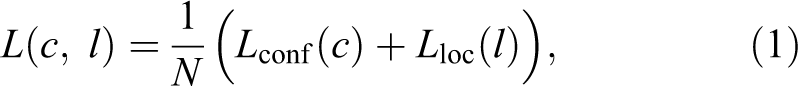
for N predictions of confidence score c and spatial offset l made by the detector. Since objects of our interest are of approximately the same size, we do not regress the height and width of the bounding boxes, which simplifies the localization loss compared to the original SSD as follows

$L_{\text{loc}}\left(l\right)={\displaystyle \sum }_{i,j}{\displaystyle \sum }_{mϵ\left\{cx,cy\right\}}{x}_{i,j}{\text{smooth}}_{L_1}\left(l_i^m-{\widehat{g}}_j^m\right),$

2

${\widehat{g}}_j^{cx}=\frac{g_j^{cx}-d_i^{cx}}{s},{\widehat{g}}_j^{cy}=\frac{g_j^{cy}-d_i^{cy}}{s},$

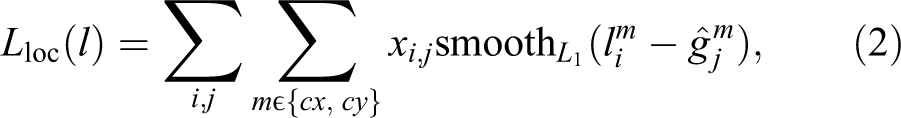
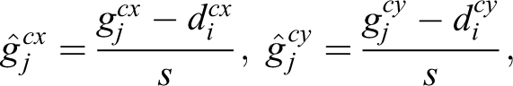
where i goes over all indexes of default bounding boxes (detector’s default locations) and j goes over all ground truth bounding boxes (object locations), x_i,j is an indicator function matching default bounding box i to the ground truth bounding box j. ${\text{smooth}}_{L_1}$ is a robust L₁ loss used in fast R-CNN detector, ³² g and d are the coordinates of the ground truth locations and default (bounding box) locations, s denotes the predefined size of all bounding boxes (64 pixels). Eliminating regression of bounding box sizes speeded up convergence of the training procedure.

The confidence loss is the cross entropy with the softmax function computed for 2 categories only, the background and the object (tip cell):

$L_{\text{conf}}\left(c\right)=-{\displaystyle \sum }_{i\in \text{Pos}}\text{log}\left({\widehat{c}}_i^{\text{obj}}\right)-{\displaystyle \sum }_{i\in \text{Neg}}\text{log}\left({\widehat{c}}_i^{\text{obj}}\right),$

3

${\widehat{c}}_i^{\text{obj}}=\frac{\text{exp}\left(c_i^{\text{obj}}\right)}{\text{exp}\left(c_i^{\text{obj}}\right)+\text{exp}\left(c_i^{\text{back}}\right)},{\widehat{c}}_i^{\text{back}}=\frac{\text{exp}\left(c_i^{\text{back}}\right)}{\text{exp}\left(c_i^{\text{obj}}\right)+\text{exp}\left(c_i^{\text{back}}\right)},$

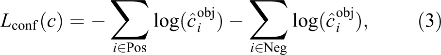
where Pos and Neg are the sets of indexes of default bounding boxes that matched ground truth object or remained unmatched, respectively. Only a part of unmatched default bounding boxes (negatives) are used in objective function as described in section Hard Negative Mining. ${\widehat{c}}_i^{\text{obj}}$ and ${\widehat{c}}_i^{\text{back}}$ are the confidences of an object (tip cell) and background, respectively, computed by the detector for default bounding box i.

Data Augmentation

Since our annotated data set is relatively small (see section Annotated Dataset of Retina Flat-Mount Images for details), it was crucial to perform extensive augmentation of the data. In addition to a set of photometric and spatial augmentations carried out by the authors of the SSD, we augment the data with rotation at a random angle in the range [0-360). Since the size of tip cells does not vary significantly, we reduced the range of the random crop sizes suggested for the SSD to [0.66-1] and used zoom-out strategy that reduces objects sizes by the factor in the [1-1.3] range.

Hard Negative Mining

In the SSD approach, negative examples are default bounding boxes that do not match object labels. Since usually there are many more negative examples than labeled positives, the authors of the original SSD used a procedure called “hard negative mining” that reduces such an imbalance. According to this approach, only a part of the negatives is selected, namely the most informative cases for the training (ie, the “hard” negative cases that may resemble a tip cell). The selection of hard cases is based on the loss function. The details on the exact procedure of the hard negative mining can be found in the original SSD paper. ²⁷ We adopt the hard negatives mining procedure using the same ratio of 3:1 between negative and positive examples. We, however, also exclude large black parts outside of the cloverleaf-like flat mount area (see Figure 3) from the pool of potential locations for negative examples. This way, we put an emphasis on differentiation between various vascular structures in the retina and tip cells, rather than between the black background and tip cells.

For this purpose, we used the binary flat mount masks generated as described in section Annotated Dataset of Retina Flat-Mount Images. Additionally, border regions of retina flat mount areas were excluded from the pool of potential locations for negatives. Due to the preparation of retina flat mounts, these regions contain cut vessels that can resemble tip cells. We therefore applied morphological erosion to flat mount masks with a square structuring element of 129 pixels per side.

Postprocessing

The trained tip cell detector may also identify tip cells at the ends of leaves of the cloverleaf-like flat mount region. These tip cells are of no interest for us, because they reflect developmental retinal angiogenesis instead of revascularizarion of the damaged retina. We, therefore, add a postprocessing filter that suppresses detections that are too far away from the retina center.

For this purpose, we calculate centroid and radius of the circle that encloses retina in the flat mount masks. To speed up computations on the large masks of 5120 × 5120 pixel size, we make calculations from its edges, which are obtained by means of internal morphological gradient. ³³ The radius is estimated from the histogram of the edge distances from the centroid. Namely, we take a radius that equals the distance giving us a maximum value of the histogram. Finally, we suppress all detected tip cells that are at the larger distances than the estimated radius reduced by a constant, which was set to 300 pixels (375 μm).

Results

System Performance

The system performance was evaluated using a separate test set consisting of 25 flat mount images of 5120 × 5120 pixel size and reference labels, which were generated by a human expert (N.Z). N.Z. is the same expert who also provided labels for the training data set (see section Data Sets for details). We will refer to this expert as the reference expert.

Figure 2 illustrates how our system performs qualitatively in comparison to the reference expert. Figure 2A shows an example of retina flat mount image with tip cells labeled by the reference expert. Figure 2C shows the same image with automatically detected tip cells. It is evident that the system identifies tip cell within the same regions as the reference expert does. The zoomed-in regions of the retina are shown on the right and visualize details of reference expert labels (Figure 2B) and automatic detections (Figure 2D). In the majority of cases, detections match the reference labels. Additionally, the examples show a few cases of tip cells that were not identified by the system, and conversely, a few structures that were not labeled by the reference expert but were detected by the system. An analysis conveyed by the reference expert has pointed out that a majority of the latter detections (not being a part of labeled tip cells) are in a gray-zone, that is, cannot not be decisively assessed. In addition, some of the novel detections were actually overlooked during the labeling process.

The detector outputs locations of tip cells and corresponding detection confidences in the [0-1] range. We quantitatively evaluated its performance using a precision-recall (PR) curve, which is commonly used for performance estimation of such detectors. The curve shows the trade-off between precision and recall values with varying detection threshold. Precision indicates the number of true detections relative to the number of all detections, while recall (or sensitivity) indicates the number of correctly detected objects relative to the overall number of objects of interest.

Figure 5 shows the PR curve for our case of the tip cell detector, when we defined a localization tolerance, equal to 64 pixels (80 µm), that sets an allowed maximal distance between predicted and ground-truth tip cell locations. A detector can operate at any point on the PR curve, which is defined by a chosen threshold on detector’s confidence. We empirically set the confidence threshold to 0.35, which corresponds to the operating point shown in red in Figure 5. An average precision is frequently used to summarize the PR curve with a single value in order to compare systems in a simplified way or to track improvements in performance at every step of a training process. Average precision equals to the mean of precision values over the range of recall values, which in our case reaches 0.90.

Figure 5.

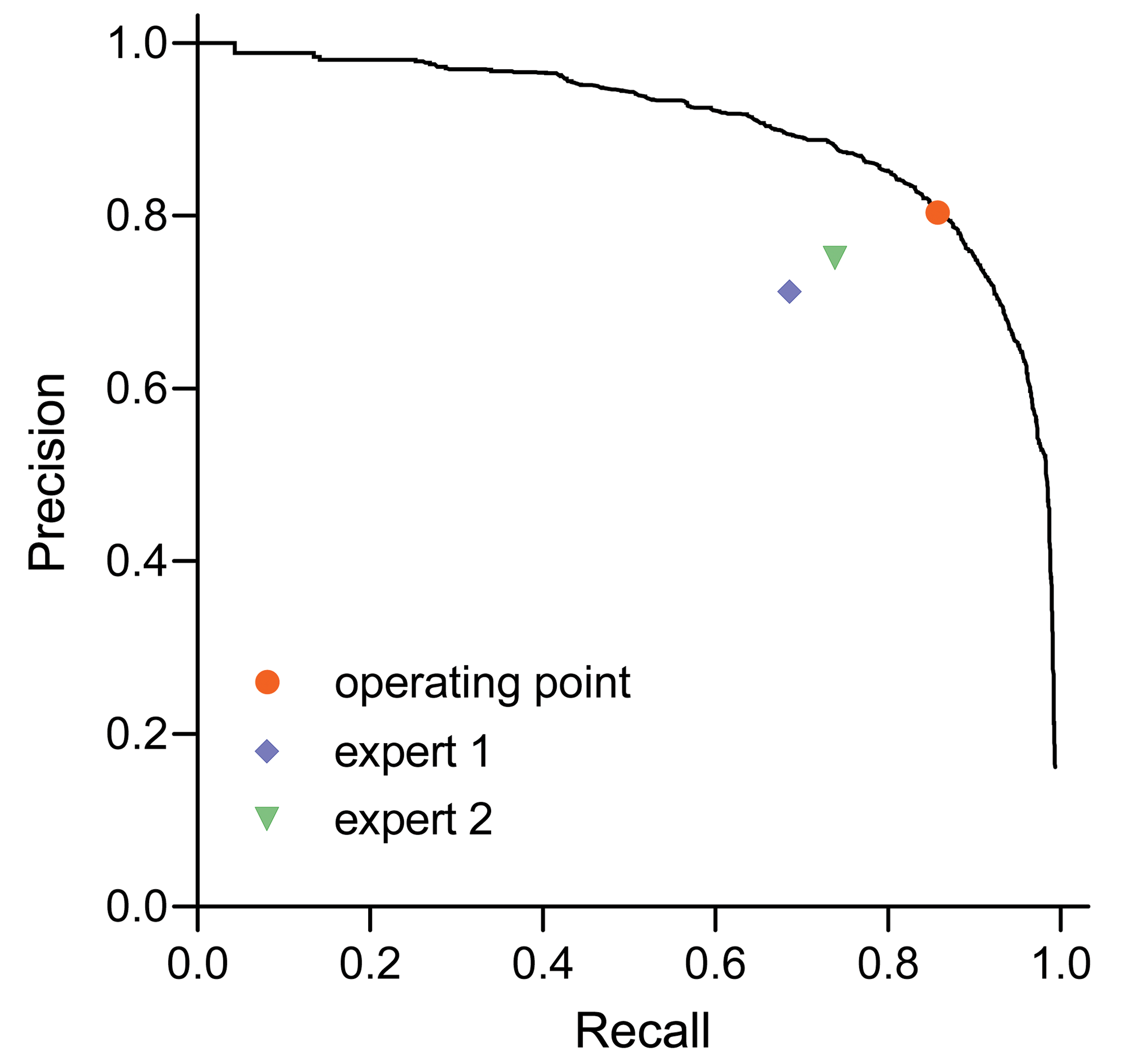
Precision-recall curve of the deep neural network (DNN) detector, chosen operating point of the detector, and comparative performance of human experts.

To the best of our knowledge, our system is the first tip cell detection system, and we therefore compare the performance of our tip cell detector to performance of the current state of the art: human experts. For this purpose, the reference expert (N.Z.), who has an extensive experience in the field, trained 2 biomedical experts (T.S. and S.T.) to manually label tip cells in flat mount images according to the same guidelines.

T.S. is a veterinarian with a proven track record in histological evaluation of organs including eye/retina. S.T. is a trained technician with experience in sprouting angiogenesis. The performance of biomedical experts in predicting the tip cell locations in the test set was measured in terms of precision and recall pair values, which are depicted as points in Figure 5 together with the PR curve for the trained system. The figure shows that our system is superior over the human experts in detection and localization of the tip cells.

Comparison of Tip Cell Counts

Our system was built to automate tip cell counting in retina flat mounts. We therefore analyzed the correlation between the number of automatically detected tip cells (orange markers in Figure 6) and counts calculated from reference expert labels (n_ref). Figure 6 shows that the counts are indeed highly correlated, which is quantitatively expressed with a Pearson correlation coefficient r = 0.94 and the average relative difference $\frac{|n_{\text{ref}}-n_{\text{det}} |}{\left(n_{\text{ref}}+n_{\text{det}}\right)/2}$ of only 11%. As we did for the performance estimation in the System Performance section, we also compared the correlation of our system with the reference expert labels versus the correlation of 2 further human experts (blue and green markers) with the reference expert labels. Again, the counts based on the automatic detections have a considerably higher correlation with n_ref then the human expert counts. The figure also clearly shows a high annotation variability between experts (interobserver variability). The counts of biomedical expert 1 and expert 2 are correlated with a Pearson coefficient r = 0.56, that is, 2 human experts show considerably higher variability than the DNN detector compared to the reference expert (r = 0.94). The average relative difference between 2 biomedical experts $\frac{|n_{\text{exp}1}-n_{\text{exp}2} |}{(n_{\text{exp}1}+n_{\text{exp}2})/2}$ equals 33%, again much larger than between the DNN detector and the reference expert (11%).

Figure 6.

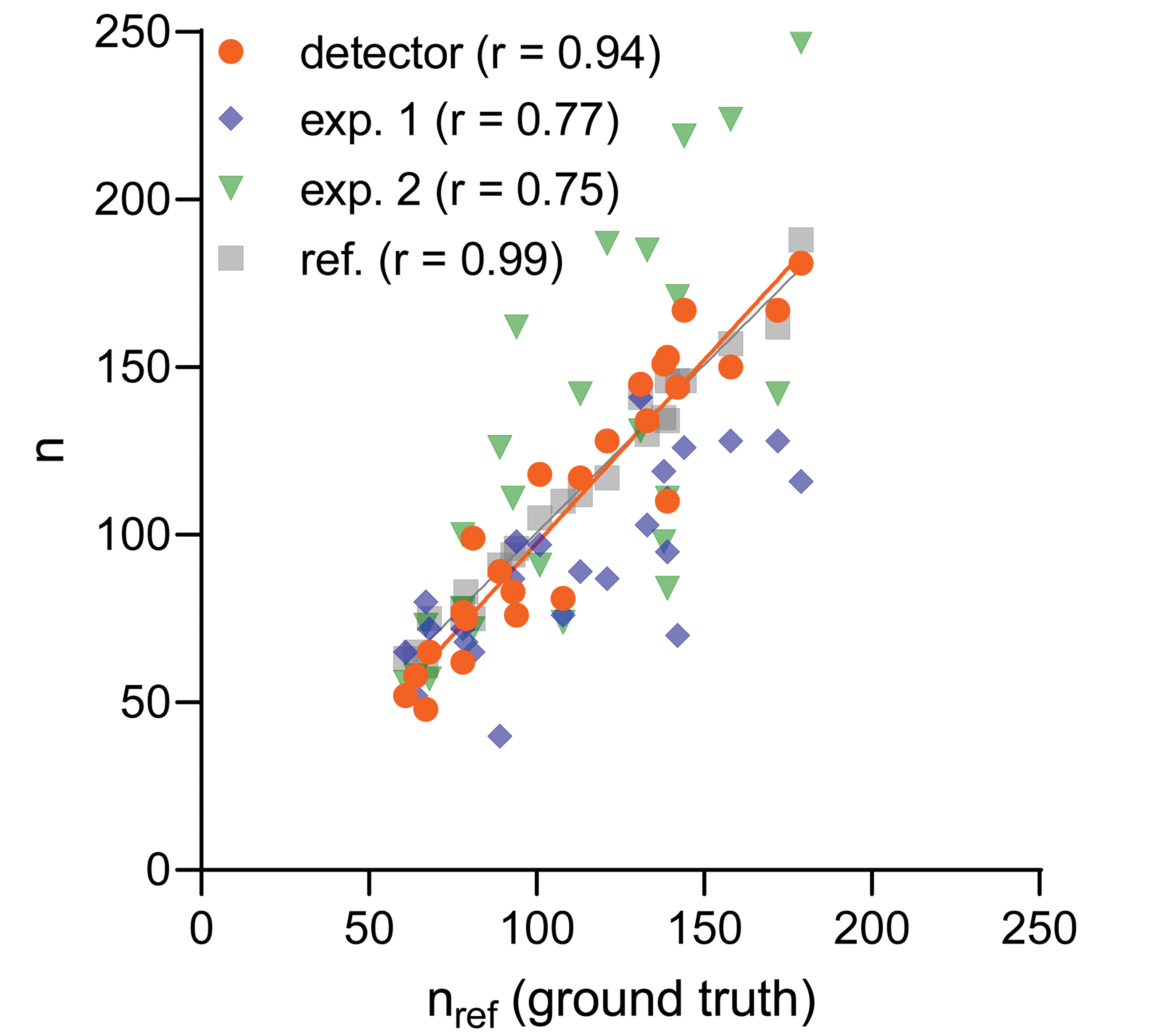
Correlation between the number of tip cells counted by a reference expert n_ref and detected automatically with deep neural network (DNN) detector (orange), as well as a few test experts (blue and green). Gray data points were obtained from the tip cells labeled by the reference expert in the repeated attempt (one month after the first attempt). The detector was trained on a separate (training) data set of retina flat mount images annotated by the reference expert. r denotes Pearson correlation calculated from 25 data points (the number of flat mount retina images in the test data set), solid lines are obtained with linear regression from the corresponding data points.

To assess the quality of the counts of the reference expert and the consistency of human labeling (intraobserver variability), we asked the reference expert to label the same test data set again, one month after the first attempt. Gray markers in Figure 6 show the resulting counts, which turned out to be highly correlated (r = 0.99) with the counts of the first labeling session. This indicates a high quality of the labels provided by the experienced reference expert. It should be noted that with the automatic system we have a counting consistency that would be quantified with the correlation r = 1.0, since it will score always identically (as long as the DNN model is kept constant). From Figure 6, we can observe that the regression lines for the counts from the repeated labeling effort of the reference expert and from the DNN detector largely coincide, which suggests that our tip cell detection system can substitute for human annotation.

We, additionally, did an experiment comparing detected tip cell counts in 32 flat mounts captured with a Zeiss LSM and an Opera Phenix HCS system. Flat mounts were prepared at different years in comparison to the training and test data sets. The flat mount preparation was performed according to the same protocol as previously. In contrast to the images acquired with the LSM, image acquisition with HCS system was performed after one year storage of the flat mounts, which might have reduced their fluorescence intensity. To cope with very different illumination conditions and exposure times, brightness of all the images was linearly adjusted to match average brightness of the images in the training data set. An analysis of the tip cell counts detected in images acquired by the 2 systems resulted in a Pearson correlation coefficient of r = 0.86 (n = 32), see Figure 7. This shows the robustness of our system in detecting tip cells using images acquired with different devices, or under different acquisition conditions. However, as shown in Figure 7, the system detects slightly more tip cells in the images from the HCS system compared to the LSM, presumably due to slight differences in focal depth or optical resolution.

Figure 7.

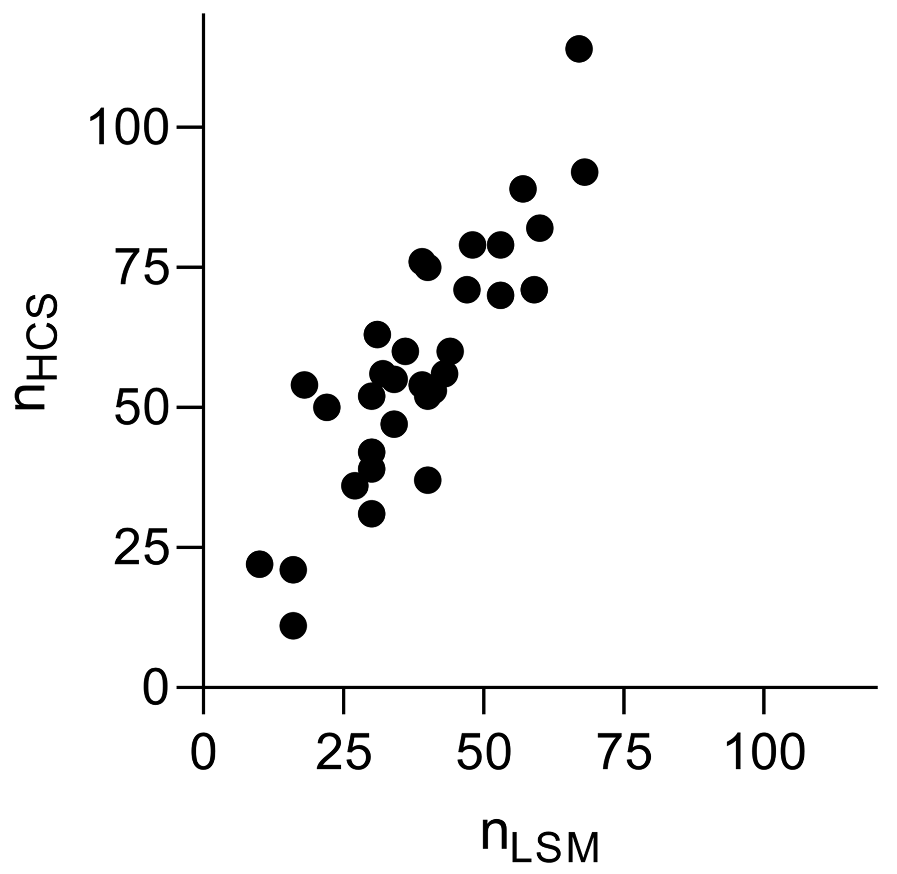
Correlation between the number of tip cells detected in the images acquired with the Zeiss laser scanning microscope (LSM) and Opera high-content screening (HCS) systems. The Pearson coefficient calculated from 32 data points was r = 0.86.

Therefore, in order to study changes of tip cell counts, for example, in an efficacy study, it is advisable to compare detections only on images of the same type (device, acquisition settings, and similar flat mount preparation method). Ideally, the detection system should be retrained on examples of labeled tip cells taken from the same type of device.

Discussion

We have developed a DL-based system in order to automatically detect and count tip cells in flat mount images. The system was trained on a moderate number of manually labeled flat mount images. We allowed a convenient labeling of the tip cells using the ZEN software (Carl Zeiss). Our experiments have shown that the system can confidently predict the expert’s labels on a separate test set. It was also shown that human experts do not achieve a similarly high performance. This suggests that the system can be trained in a more comprehensive and effective way compared to human performers. For this study, we compared the system to 2 test human experts and the reference expert labels (ground truth for training in our case). A more thorough assessment of the performance of the system compared to an average performance of a qualified human would require a larger number of test experts.

We built our system based on the deep neural SSD architecture. ²⁷ Confident detection of rather small tip cell structures contradict a commonly adopted statement suggesting that the SSD does not perform well for detection of small objects. ²⁶ As evident by our results obtained with a customized SSD, the SSD architecture is general enough to handle objects of any size, but its performance strongly depends on parameters used, the chosen configuration of feature maps, and the training data set.

Recently, a few novel object detection architectures ^34,35 were proposed that do not rely on predefined bounding boxes as SSD does and also show better results on standard benchmarks such as the MS COCO data set. ³⁶ Such approaches suggest a simpler and potentially more robust solution. In our case, CenterNet ³⁵ approach might be most advantageous and interesting for further investigation, because similarly sized tip cells are sufficiently defined by their central location and do not require usage of bounding boxes.

In case of changes of image acquisition, or if novel morphological varieties occur, which the DNN was not trained with, the system can be consistently improved by adding new training data. This ensures that the system becomes more robust and even more reliable over time. In our opinion, sharing robust and verified DNNs will be a promising way to ensure more consistent analysis results across laboratories and over time.

In summary, our system allows a fast and consistent counting of tip cells and unburdens human experts from fatiguing routine work.