
Abstract
Quantitative image analysis (IA) is a rapidly evolving area of digital pathology. Although not a new concept, the quantification of histological features on photomicrographs used to be cumbersome, resource-intensive, and limited to specialists and specialized laboratories. Recent technological advances like highly efficient automated whole slide digitizer (scanner) systems, innovative IA platforms, and the emergence of pathologist-friendly image annotation and analysis systems mean that quantification of features on histological digital images will become increasingly prominent in pathologists’ daily professional lives. The added value of quantitative IA in pathology includes confirmation of equivocal findings noted by a pathologist, increasing the sensitivity of feature detection, quantification of signal intensity, and improving efficiency. There is no denying that quantitative IA is part of the future of pathology; however, there are also several potential pitfalls when trying to estimate volumetric features from limited 2-dimensional sections. This continuing education session on quantitative IA offered a broad overview of the field; a hands-on toxicologic pathologist experience with IA principles, tools, and workflows; a discussion on how to apply basic stereology principles in order to minimize bias in IA; and finally, a reflection on the future of IA in the toxicologic pathology field.
Keywords
Digital pathology is revolutionizing the way pathologists conduct their art. While pathologists have been using the same approach for centuries to make their medical diagnoses out of a microscope, our society went through a fast, drastic revolution with the creation of the Internet 40 years ago, followed by the worldwide web and the daily digitalization of the information capture and sharing with smartphones. The advances in digital science and applications make it possible to adopt and adapt these technologies to pathology assessments. The addition of quantitative assessments to pathology has already had a significant impact in clinics for diagnosis, patient stratification, and treatment monitoring and can impact as much the preclinical area where competition and environment call for faster selection of better compounds. This continuing education session provided an overview of digital pathology progress and pitfalls, discussed workflow solutions to optimize the use of digital pathology, and how to apply basic stereological methodologies to minimize bias in image analysis (IA). Case studies with hands-on pathologist’s experience for the selection of the most appropriate technology based upon the questions to be addressed, and their application to generate relevant meaningful information was presented.
Pathology through Pixels, Where We Are, Where We Need to Be
The current status and outlook of digital pathology IA were discussed by Dr. Robert Dunstan (AbbVie, Worcester, MA). In 2006, a company brought a proposal before a major pharmaceutical company to develop a program to “accurately separate normal from non-normal tissues in multiple species (rats, mice, dogs and nonhuman primates) for up to 47 tissues and for the rapid screening of slides for histology (on hematoxylin and eosin [H&E] stained, histologic sections).” The pharma company liked the idea and was considering the investment of millions of dollars to develop this technology but requested a pilot project to demonstrate that the company could do what it claimed before a major investment was advanced.
The target tissue was the liver and after a year of meetings, revision of algorithms and trying the method on training sets, the moment of truth had arrived. A collection of 179 digitized rat liver slides (both normal and abnormal) taken largely from old toxicopathology studies were evaluated by the technology. The truth standard was defined by a group of pathologists who reviewed the images by standard microscopy and agreed with the diagnosis.
When the results were in, “Robopath” (as the method was nicknamed) had a sensitivity (the ability to accurately identify the liver sections with lesions) of 82% and a specificity (the ability to accurately identify normal tissue as normal) of 28%. These values were far too low to serve as a surrogate for visual assessment of microscopic changes. In fairness, the company subsequently claimed they made a mistake in one of the algorithms and when reassessed, the results were much better, but the pharma company decided not to continue with further discussions regarding the technology and for all intents and purposes, Robopath died.
It is now 2017 and for a decade (a very long time when one considers how rapidly technology advances) whole slide imaging and IA methods have been evolving. In 2006, very few pharmaceutical companies had whole slide imagers, and fewer were using IA methods that could even try to attempt what Robopath proposed. Now, with the Food and Drug Administration (FDA) approving the use of a whole slide imaging system for the interpretation of digitized images of surgical pathology slides and the development of deep learning methods for the analysis of these images, the interest in quantitative assessment of histologic changes has greatly increased.
Still, the cautionary tale provided by Robopath is like one of Aesop’s fables—old but still relevant—especially in 3 areas that most concern IA: (1) doing IA for the right reasons, (2) asking a question that is unanswerable by current technology, and (3) trying to solve an IA problem the wrong way.
Lesson 1 from Robopath—IA Was Done for the Wrong Reasons
Robopath was sold as a method to “enable pathologists in the pharmaceutical industry to realize immediate and measurable increases in productivity [and to] afford them the opportunity and time to optimize their value to the discovery and development of new medications.” This is the wrong reason to develop IA. Changing from a visual to a quantitative read of digitized histologic sections is neither a time nor a resource saving enterprise, at least for the present. To be blunt, currently there is no situation where digital pathology and IA result in any cost reductions in the pathology laboratory (Hewitt 2017). Just setting up whole slide imaging is both hardware and labor-intensive. A recent estimate indicates that scanning 300+ slides a day requires a full-time employee just to keep slides clean, organized, labeled correctly, scanned, and filed (along with the storage of the glass slides; Hewitt 2017; personal communication to author July 11). Adding quantitative morphometry requires time to learn the software, time to write and train an algorithm, time to validate, time to calculate, and time to graph. Finally, an IA algorithm only creates value if it informs changes that occur in a large number of samples across multiple studies. The details of digital pathology workflow solutions were discussed in the second section.
In spite of these time and cost sinks, the value of IA far outweighs its liabilities. First, it enables the standardization of histopathology by quantitation rather than by visual assessment; second, it will result in more accurate, less-biased interpretations; third, it will allow for the recognition of morphologic patterns not currently recognized; fourth, it will more rigorously tie morphologic features to molecular biology. In short, the future of anatomic pathology lies in its inevitable transition from a primarily descriptive to a primarily quantitative discipline.
Even the FDA is recognizing the value of quantitative analysis of histologic sections. In May 2016, the FDA released a “Guidance: Considerations for Use of Histopathology and Its Associated Methodologies to Support Biomarker Qualification.” To sum, the FDA recognized that the gold standard for assessment of disease was histopathology and when morphologic changes were associated with a quantified assay used as a biomarker, the two had to be correlated. The majority of the guidance then discussed the rigor to which histopathology needed to be performed and that this correlation needed to be quantitative: Biomarker qualification studies should evaluate the
Lesson 2 from Robopath—The Technology Was Not Sufficiently Advanced to Perform the Task
The sellers of Robopath claimed they could perform the analysis by using fractal-based analysis of complex structures. Fractal analysis was more widely used over a decade ago and still has value in identification of edges or texture but has largely been discarded as a dominant technology to be used for IA. In short, Robopath was doomed from the beginning. The question then becomes how advanced is IA in 2017 and could the goals of Robopath be met today?
To answer these questions, one needs some basic knowledge about how IA is performed. All current IA occurs on digital images as opposed to analogue images. An analogue image is represented by a picture taken on a standard camera with film. Here, the image is produced through a chemical reaction. There is a continuous scale of color. A digital image is one that is generated by a computer in which the image is composed of areas (normally squares) known as picture elements or pixels that are stitched together. These pixels are usually too small to be seen unless the picture is greatly enlarged and the thought is that for all intents and purposes the digital image is similar to the analogue image.
Digitized whole slide color images are based on a red, green, and blue (RGB) color model with each pixel containing an R, G, and B color value. Each of these 3 colors has 256 possible variations (28 or 8 bit) on a 0 to 255 scale. When one considers a pixel can have 256 different RGB colors, respectively, this means there are 2563 or 16,777,216 possible colors (Lloyd, Monaco, and Bui 2016). Note that in this model where the colors are additive, black is the absence of color (R = 0, G = 0, and B = 0), and white is the maximum color possible (R = 255, G = 255, and B = 255; Figure 1).

The red (R), green (G), blue (B) color model. Each color has a range of 0 to 255 colors. When all colors with a value of 255 are overlapped, the color is white. When all colors with a value of 0 are overlapped, the color is black. Note also the colors when 2 individual colors overlap: green and red produce yellow, red and blue make magenta, and blue and green make cyan.
When you look at a digitized image, you see colors, but the computer sees a matrix of thousands and thousands of pixels, each with their own R, G, and B color values. That each pixel has a numerical value means the colors you see can be manipulated by mathematic algorithms. This manipulation is called “image processing.” These algorithms can be written to remove artifacts, to identify and segregate complex structures, and lastly, because each pixel has a known area, to calculate the area of structures of interest. Two points need to be made here. First, microscopic morphology is complex, and it is not unusual for dozens of algorithms to be combined into “master algorithms” to correctly identify structures of interest. Often master algorithms are required at different magnifications. Second, IA data are invariably presented as a ratio of something desired to be quantified (e.g., area of ionized calcium-binding adapter molecule 1 [IBA-1] positive staining cells) per a known area of tissue (e.g., a liver section). As a general rule, and especially when immunohistochemistry (IHC) or in situ hybridization (ISH) methods are applied, identification of the areas that define the protein or messenger RNA (mRNA) of interest is much easier to identify and quantify than the regions of interest in which they are located. Because IA data are expressed as a ratio, errors in calculation of the numerator or the denominator alter the accuracy of the analysis equivalently.
The same mathematical algorithms serve as the basis of all IA; however, how these algorithms are applied is evolving. One way of understanding IA and its evolution is by thinking of these methods as a Venn diagram with 3 interconnected processes: (1) thresholding, (2) machine learning, and (3) deep learning (convolutional neural networks [CNNs]).
Thresholding
Thresholding serves as the backbone of IA. With thresholding, the decision as to what algorithms are used, and the range of the pixel values analyzed by these algorithms is determined by the person writing the master algorithm. It is totally supervised. This is in contrast to machine and deep learning which are “semisupervised,” meaning the programmer provides input, and the computer largely decides what algorithms go into the “superalgorithm.” True unsupervised methods where the computer analyzes images without any training are seldom used because at present they are less efficient.
Thresholding generally occurs in steps that vary depending on the software, but all involve the same basic processes. Step 1: Setup. This is where the magnification for the analysis is selected. Also defined in this step is whether the whole image is to be analyzed or what fraction of the image is to be analyzed by random selection. Step 2: Preprocessing. Here filters used to analyze the image are selected. These filters can define features of the image based on color(s), texture(s), hue, saturation, and/or intensity. Polynomial filters can enhance edges, and mean filters can decrease complexity. Note that all of these filters can be combined with each other to compound their effects. The preprocessing steps also transform the image to gray scale. Step 3: Classification. In this step, the specificity of the filters to be used is improved by limiting the range of the grayscale values. Step 4: Post processing. This occurs after the preprocessing and classification steps have been applied and “fine tunes” the image by separating classified labels further based on features like size, shape, and intensity. Step 5: Calculation. In this step, the labeled pixels are given numerical values based on the criteria to be quantified such as area, intensity, or perimeter.
As already stated, thresholding often requires multiple algorithms. The first algorithm usually identifies the tissue(s) to be analyzed at the lowest possible magnification. The second algorithm may subdivide the tissue into anatomically important regions at a higher magnification. The third algorithm may quantify cells of interest in the anatomically important regions, which is often done at 10× to 40× magnification depending on the resolution needed.
The way thresholding works through preprocessing and classification is that each filter uses a structural element (also called a kernel) that consists of set pixel dimensions. As a rule, the length and width of the structural element are both odd numbers (i.e., 3 × 3 pixels, 21 × 21 pixels) so there will be a single central pixel. This structural element then goes over every pixel in the image, changing the image as directed. This will first change the colored image to a gray scale, usually emphasizing RGB colors or hue, saturation, and intensity. The grayscale image is further modified by drawing information from the surrounding pixels defined by the structural element and applying them to the central pixel (Figure 2).
The use of structural elements to process images. All figures are of a 5× magnification area of human epidermis stained with hematoxylin and eosin (H&E). A and E represent the region of interest to which different pixel structural elements were applied. Note that the boxes in the pixel element are larger than the true pixel size because the image is at 5× magnification and the images were captured at 20×. B represents the mean 0 to 255 value of a red color filter defined by a 3 × 3 square structural element in each of the boxes. C depicts the grayscale image when the red filter was applied to a larger area of the image. D represents the H&E image of C. F is the same region as B, but a 3 × 3 square mean filter was applied. Here, the central 0 to 255 value in the center square is the average of the 9 pixels. G depicts the grayscale image when the mean filter was applied to a larger area of the image. H is the same region defined by G, but an 11 × 11 square structural element is applied. Note how the complexity of the image is reduced by the larger structural element.
The use of thresholding remains a powerful means to create robust algorithms. Thresholding algorithms were most commonly used in pathology IA (see Table 1). In addition to sophisticated software packages, many user-friendly packages as discussed in the third section (cases 1–4) of this article utilize thresholding algorithms. In the hands of an experienced programmer, it will often outperform machine-learning methods because of the application of post processing steps. However, getting to the point where a programmer can maximize the effectiveness of thresholding requires considerable training and practice.
A Sampling of Recent Publications Using Thresholding, Machine Learning, and Deep Learning (CNNs) for Tissue IA.
Note: The publications were selected from many to demonstrate the diversity of projects using IA, their complexity and how broadly IA methods are being incorporated in the histologic assessment of whole slide images. They were also selected because the current “state of the art” of thresholding and machine learning tends to be based on quantitation of IHC expression in a region of interest. In contrast, CNNs are being developed on H&E-stained sections and are tending to be more “diagnostic” and structurally based. IA = image analysis; CD = cluster of differentiation; PD = programmed death; PDL = programmed death ligand; CNN = convolutional neural network; IHC = immunohistochemistry; H&E = hematoxylin and eosin.
Machine learning
Machine learning uses the same basic algorithms as thresholding, but in a way that the computer performs its analysis without being explicitly programmed to do so. Thus, it crosses into “artificial intelligence” where the computer is able to “teach itself.” The best examples of machine learning are those programs that use a “paint by numbers” approach in which the programmer draws a colored label over different areas desired to be separated from one another, and the computer “magically” separates the regions. Because of the complexity and variation of the histologic images, often multiple sites have to be labeled to train the computer.
There are multiple behind-the-scenes ways that do this “magic”: k-means clustering and random forest classifiers to name two. Only random forest classification will be discussed here because it is the most widely used. The reader is referred to other references for additional information on this topic (Lloyd, Monaco, and Bui 2016; De Freitas 2013; Blackwell 2012).
The random forest classifier is based on the “wisdom of crowds.” In 1907, the statistician Francis Galton visited a county fair where attendees were asked to guess the weight of an ox to receive a prize. There were 787 guesses, the mean weight of the guesses was 1,197 pounds; the actual weight of the ox: 1,198 pounds. This “coincidence” fascinated Galton who determined (1) if there is a diversity of opinion; (2) if the opinions are from those with a range of knowledge; and (3) if the opinions are not determined by those around them, then crowds of people can make surprisingly good decisions in the aggregate even if they have imperfect/incomplete information (Harvard 2011). Another example of this is the television show “Who wants to be a millionaire” where the “ask the audience” lifeline was correct 91% of the time; the “phone a friend” lifeline answered correctly only 62% of the time (http://millionaire.wikia.com/wiki/Ask_the_Audience).
Random forest classifiers use this method of analysis through a decision tree: a graph that looks like an upside-down tree that is used to predict statistical probability (Figure 3). To understand this, we start with an imaginary image in which with each pixel has been graphed in 3 dimensions based on its RGB coordinates. For simplicity, “painting by numbers” has been applied and has separated pixels into 2 groups defined by yellow and blue spheres. Note that the yellow sphere has a red “X,” and the blue sphere has a purple X. These represent centroids and are the geometric center of the clustered pixels. Now suppose the next pixel is intermediate between the blue and the yellow spheres. How is a random forest classifier used to determine which of the 2 groups in which it should be placed?
An example of a hypothetical decision tree applied in Figure 4.
This starts by having the computer design a decision tree. The lines are called branches, the internal boxes are called nodes, and the terminal boxes are called leaves. The computer then randomly selects a subset of the pixels in the yellow sphere and a subset of the pixels in the blue sphere and determines the centroids for these subgroups. The closest centroid to the purple pixel “wins.” This is then repeated multiple times with a different selection of pixel subgroups. Because the tree is used over and over again it results in a mathematical “forest” (even statisticians can have a sense of humor). In the end, a decision is made by the answer that comes up the most on the different trees (in this hypothetical case, it is the blue-labeled pixels; Figure 4).
The application of the decision tree in Figure 3. There are 2 pretrained clusters of pixels based on their red, green, and blue values. The centroids of the pixels defined by the yellow and blue spheres are defined by a red and purple “X,” respectively. The computer now comes across an unclassified pixel (defined in purple) and needs to decide whether it is best placed in the yellow or red group. This is done by randomly subsampling a subset of pixels in the yellow sphere and a similar subset from the blue sphere. The tree is applied, and a centroid is calculated from each of these subsets with the centroid closest to the unclassified pixel considered to be the “winner.” The process is repeated over and over again giving with the trees in aggregate giving the appearance of a forest. The final location of the pixel is decided by the majority of the decision trees, indicating that the pixel belongs in the yellow or the blue spheres.
The use of random forests makes complex IA quite easy because regions of interest can be separated by merely applying labels. However, like all IA methods, it is not a perfect solution, and it too has limitations. First, for segregating complex images, especially when there is little color or textural differentiation, it is possible to “oversample” with machine learning, eventually drawing so many lines that the computer gets confused. Second, the algorithms used to analyze the tissues are largely invisible to the programmer. This is in contrast to thresholding where all the parameters used for the algorithm are known. Thus, it is difficult to see mistakes and to correct them. In short, it is much easier to use thresholding to duplicate an algorithm produced by machine learning than it is to use machine learning to duplicate an algorithm written by thresholding.
Machine-learning algorithms, particularly random forest, have been applied for pathology IA (Table 1). These algorithms have also been incorporated in commercially available user-friendly software packages (as discussed in the third section of this article).
Deep learning/CNNs
Deep learning can be viewed as a more advanced method of machine learning with predictive capabilities that mimic the human brain. Its advantage over more conventional machine learning is that it is resistant to small changes and can generalize from partial data sets. For example, if one uses an image of a classic lymphocyte, changing a few pixels will not change a pathologist’s ability to recognize that the image is a lymphocyte. This is how deep learning works. With appropriate raw data input, it will be able to establish criteria for what a lymphocyte is and apply them even when presented with a morphologic variant upon which it has not been specifically trained. In the end, with proper training, deep learning is superior to other methods in speed and accuracy.
Analysis by convolutional neural net starts with input images. These consist of “truth standards,” that is, a large series of images each comprised of a known morphologic entity, say, lymphocytes (note that the accuracy of analysis also requires the computer is trained to recognize those cells that are not lymphocytes).
Each input image is broken down into smaller parts, say groupings that are 100 × 100 pixels. The computer will then analyze them by applying dozens of different filters (using structural elements just like those used for thresholding) across the image, a process known as convolution. These filters identify features of the image such as straight edges, colors, and curves.
The next step is called pooling. In pooling, the complexity of a filtered image stack is reduced by using a new, often larger structural element that selects the pixels with the highest 0 to 255 value across the filtered images. At this stage, the program identifies features, but they are small lines and curves and color-based textures. Now a second convolution is applied, using the features identified in the first convolution layer. This allows the program to identify more complex features such as semicircles or nucleoli. Another pooling step may be applied, and this process is repeated again and again over all the lymphocytes (usually hundreds) in the training set.
The convolved, pooled images are then combined into a fully connected layer where data are combined and the hundreds if not thousands of features that make up a lymphocyte based on the training set are defined. When a new lymphocyte is exposed to the program, the computer weighs all the features that make up a lymphocyte against the features the computer has been trained to recognize what are not those of a lymphocyte. If the majority of the features suggest a lymphocyte, then the final stage, the output stage, makes the call that the cell is a lymphocyte. If the majority of the features do not favor a lymphocyte, then the cell is rejected.
The author recognizes this is a very simplistic overview of a complex method and ignores features that improve the accuracy of analysis like backpropagation or gradient descent. The reader is referred to other sources for more detailed information on CNN (Roher 2016; De Freitas 2013; Tajbakhsh et al. 2016; Wang 2016; Deshpade 2016; Granter, Beck, and Papke 2017; Beleites et al. 2013).
The use of deep learning/CNN is still too new to decide what role it will play in the morphologic assessment of microscopic changes, but if one realizes that it serves as the basis of facial recognition, there does appear to be a great potential for application to anatomic pathology and to allow for the recognition of complex structural patterns that we have been unable to capture. At the same time, this requires coding skills by the programmer and considerable computer power to implement.
Lesson 3 from Robopath—The Images Were Extremely Difficult to Analyze
There are many reasons why Robopath failed, but one major reason is that those selling the technology and its evaluators naively assumed that writing a robust algorithm with the methods proposed was going to be trivial, so trivial that it the software could be applied to multiple organs across multiple species dealing with multiple disease morphologies. We were wrong. Lessons learned from this, and other projects over the decade have taught that writing an IA algorithm that can be used across studies is never trivial; however, the following steps can be taken to greatly improve chances for success.
Standardize methods
Making the switch to computer-based IA allows the pathologist the opportunity to quantify the large impact staining variability and artifacts such as tears and folds have on writing an IA algorithm—features that are typically read through when the evaluation is visual. Even on well sectioned slides almost invariably, there will be an “artifact removal algorithm” to correct for these changes. Thus, the first step to ensure IA success is to standardize every step in tissue handling to minimize pre-analytic variability. This includes cold and warm ischemia, fixation time, tissue thickness at harvesting, orientation during trimming and embedding, processing, sectioning, staining, and scanning (different scanners, especially those by different manufacturers, have variability in color, magnification, and pixel density [the area covered by a single pixel]).
Improve contrast
An objective of performing IA is to make the algorithm easy to write and highly reproducible. This can best be performed if a priori, staining is optimized to allow for high contrast of the regions of interest and high contrast of the areas needed to be quantified within the region of interest (ROI). The standard is to use a monocolor stain such as hematoxylin as a counterstain and a single IHC chromogen. For complicated analyses of tissues, this is often not enough to allow for accurate, reproducible, quantitation where polychromatic histochemical stains such as periodic acid–Schiff (PAS) or Alcian-blue PAS with dual IHC will greatly improve the accuracy of the analysis (Figure 5). It can take time to optimize a staining method that highlights the areas you want to quantify, but it is well worth the effort.
The image is of rat colon demonstrating the value of increasing the contrast to perform image analysis. A represents the stained image where the mucosa is defined by immunohistochemistry (IHC) staining for EpCam (red), the smooth muscle is defined by IHC staining for α-smooth muscle actin, the goblet cells are defined by Alcian-blue periodic acid–Schiff staining. (B) Is the analyzed image. Yellow and unlabeled regions represent nonepithelial tissues. Blue represents nonmucus nuclear and cytoplasmic regions of enterocytes. Green and red represent goblet cells of different sizes. Using stains that highlight the contrast among the regions to select, deselect, or quantify makes the writing of an algorithm much easier as well as more reproducible.
For new algorithms, always do a pilot project first
It is important that you know the challenges and that you have time to consider methods to standardize and to improve contrast. Always write the first algorithm on a pilot project or a smaller training set before tackling a large, important study.
A single study does not a make robust algorithm
A goal of any algorithm should be its application with accuracy across multiple studies. To do this, the algorithm has to be able to capture the maximum range of pre-analytic variability and the range of biologic variability. To insure this is captured, an algorithm needs to be applied across regions, slides, and studies. A rule of thumb is that a minimum of 100 slides and a minimum of 5 studies need to be analyzed.
IA should not violate basic principles of stereology
Often stereology is viewed as the more manual cohort of IA. In reality, stereology remains the gold standard of quantitative morphology regardless of the method used. One should realize, for example, that when we say 10% of the area of a liver consists of IBA-1 positive macrophages, one is really saying that area and volume are precisely related and that 10% of the volume is also consists of IBA-1-positive staining cells. This is usually not confirmed but can be if the block is sectioned through its entire thickness at a consistent and known distance. Two other rules that are often violated include “cherry” picking, where areas for calculation are sampled because “they look good.” One is under no obligation to analyze an entire section of tissue; in fact, usually this represents analyzing more tissues than one needs for statistical separation. However, if one subsamples, there is a need to do the subsampling using valid stereological methods such as systematic uniform random sampling (SURS; see Reducing Bias in IA by Applying Stereological Principles section). The second common violation is defining expression by counting rather than giving an area percentage. Number estimations using stereology require the use of a volumetric probe (known as the disector), and attention is paid to make sure one is not double counting an object. In the vast majority of cases, if one gives a count estimate and compares with area percentage, the statistical differences are minimal; however, there is a right way and a wrong way to do IA and cherry-picking and performing counting estimates without applying stereology principles is never wise.
There is an allure to performing IA on H&E-stained sections. It is the standard stain for visual histologic diagnosis. However, sections so stained are often difficult to analyze in large measure because H&E is largely low contrast. When Robopath was proposed, the computer analysis of H&E sections was just beginning. Even now, defining all the morphologic changes on an H&E-stained section is difficult and seems best suited to analysis by CNNs. This is why H&E is the stain used in the Camelyon Challenge, an international contest where entrants are asked to define a lesion on digitized images. Yet even today, it would take an incredible effort to accomplish what Robopath claimed was possible in 2006, and there would be a serious question as to whether the high cost would be proportionate to the benefit.
Where are we and where do we need to be as pathologists in a digitized world with increasing capabilities in IA? At present, there is good, powerful software available to take advantage of both thresholding and machine learning. Deep learning as exampled by CNNs, arguably the future of IA, at present is not “plug and play” and requires coding as well as the use of computers with graphics processing unit capabilities. At the time of this writing, most pharma pathologists are just beginning to evaluate its potential or are outsourcing work done by deep learning to the few contract research organizations that are skilled in its use. Published studies also point out that deep learning and neural networks are making significant progress in tissue IA (Table 1). Pathologists should remember that the technology is evolving rapidly, and it is expected methods using neural networks will become more efficient and simplified.
Through pixels, we are now primed for the greatest change in the discipline of pathology since the development of the microscope. A case can be made that the largest untapped source of novel information in the biomedical sciences is on a histologic section. With the evolving methods of analysis, we can now quantify the structural nuances that better define a disease, and we can better connect morphology with the upstream events that are captured by molecular biology. This means that anatomic pathology will change but will change for the better.
Digital Pathology Workflow Solutions for Preclinical Assessment
Digital pathology offers great potential to drive preclinical research, allowing scientists to collaborate remotely and to acquire, objectively quantify, and perform quality control of data from tissue-based assessments. Digital pathology is not limited to whole slide images (WSIs) or images taken at the microscope; it includes digitized macroscopic images, electron micrographs, and 3-dimensional (3-D), cleared whole tissue sections. This presentation by Vanessa Schumacher (Roche Pharmaceutical Research and Early Development Basel) focused on integrating workflows using digital WSIs. Digitizing slides and storing in an image management system (IMS) allows for tracking and retrieval of image metadata and permanent storage. In addition, a slide database can be a platform for sharing of slides between the laboratory, pathologists, and research scientists allowing opportunities for telepathology and collaboration.
There are many advantages to digitizing pathology slides, including increased efficiency, remote slide review (decreased travel and shipping costs and time, worldwide access to pathologists and experts), ability to store and annotate slides in a central database, and avoidance of slide loss or breakage (reviewed in [Al-Janabi, Huisman, and Van Diest 2012; Farahani, Parwani, and Pantanowitz 2015]). In addition, digitization of whole slides is the first step to digital IA, including computer-assisted diagnosis through machine-learning approaches. The concept of high-content pathology brings the added value of integrating digital pathology readouts with high-content screening, imaging biomarkers, and pathology informatics among other quantitative data for n multiplexed data approach (McCullough et al. 2004). Integration of the sample metadata with the digital slide makes the slides searchable by key word and allows for the buildup of a robust database. An all-digital, paperless archive is an efficient tool that is already being used in hospital pathology practice (Huisman et al. 2010; Stathonikos et al. 2013). An integrated workflow concept for a preclinical pathology laboratory is shown in Figure 6 as an example. Individual sample tracking and machine–machine communication are used to reliably track samples from the tissue to the slide or digital image level. Digital images are stored in a database that communicates with a database where all metadata is held. Digital workflows for various needs in diagnostic and pathology have been previously published (Bertram and Klopfleisch 2017; McCullough et al. 2004).
Example digital pathology workflow. An integrating workflow using a laboratory information system communicating with laboratory equipment and an image management system, where digital slides can be viewed and annotated.
Despite the potential benefits, digitization of whole slides has not become well integrated in preclinical pathology due to a number of factors including high cost and more resources needed to digitize slides, need for capacity to store digital images, and other workflow changes. In addition, the available options for all steps in the digital workflow are vast, and the number of publications related to digitization of toxicological pathology slides, in particular, is limited.
Workflow Steps
When integrating a digital pathology workflow, consideration needs to be given to quality control and controlling causes for variation as much as possible. There is currently no universal quality assurance plan for validating preclinical digital pathology systems; however, there are guidelines for validation of WSI systems and workflows in the nonregulated and regulated preclinical and clinical diagnostic environments (Long et al. 2013; Pantanowitz et al. 2013). Thirteen percent of WSI need to be rescanned due to issues such as lack of focus or presence of artifacts, making it logical to build in controls to check for quality of scans before continuing on to the next step in the workflow (Campbell et al. 2012). Automated slide inspection could be integrated at this time to ensure staining quality and lack of artifacts before progressing to the next step (Ying and Monticello 2006). In order to ensure proper data transfer, machine–machine and machine–laboratory information system (LIS) communications can be built in to avoid manual intervention and potential for error. Importantly, predigitization sources of variability must be controlled as much as possible, and assessment of inter- and intraassay variation is essential for optimal interpretation of quantitative IA results downstream. Automation of as many steps as possible and inclusion of appropriate controls in every staining run are methods used by some laboratories. Biologic variability must also be taken into account; for example, variation between serial sections of a tissue or variation between animals in a group. An ideal IA workflow begins at the study design phase and includes a pilot experiment to control for sources of variability.
Whole Slide Scanners
Slide scanners vary in their method of image capture, bright-field versus fluorescent (or both) throughput, flexibility of slide loading, and output of image file formats and file sizes. The most appropriate scanner to integrate into a digital workflow depends on the type of slides produced in the laboratory, the throughput and speed needed, and flexibility required. Consideration needs to be given to the integration of image file formats into downstream IA or slide viewing platforms. A laboratory that has a high throughput with continuously changing priorities would benefit from a high-throughput scanner with a continuous loading feature, while a pathologist working remotely might only require a single slide scanner. A laboratory that requires digitization as part of its workflow should strongly consider having a backup instrument in case of breakdown of one scanner, to prevent disruption of the workflow. An overview of slide scanning technologies and options is detailed by Farahani, Parwani, and Pantanowitz. Scanning magnification requirement depends on the downstream applications. Analysis of large structures may require only 10×, pathology evaluation, and ISH IA requires at least 40×, and 60× is required for cytology preparations. Routine scanner calibration and scanning standard operating procedures are recommended to reduce variation, and scanners utilized for Good Laboratory Practice studies may need to be validated. Slides must always be cleaned before scanning to avoid dust and oil artifacts.
Special considerations for fluorescent scanning include building in appropriate controls to ensure no cross talk between channels and defining of the optimal exposure time and filter settings. In establishing multiplex assays, the singleplex stains should always be included in the establishment runs to control for this as well. It is recommended to save a protocol for a specific staining setting, and to always include appropriate controls in the staining run to ensure accuracy, especially when using scanning results for quantification. Based on the stability of the fluorophores used, the slides should be scanned within a defined time frame to avoid fading. This can be determined by staining serial sections of a slide and scanning each one at different time points. In addition, the time from sectioning to staining of frozen samples may have an impact on the amount of background staining observed. Every pass of the scanner will bleach the slide, so it is recommended to optimize scanning conditions on a control slide not needed for analysis and to avoid repeated scans. A control, unstained slide can be included to correct for tissue autofluorescence.
Data Management
Digital data must be stored and managed, and there are a number of commercial or open-source solutions available for digital slide management and/or slide sharing. When storing images, consideration should be given to how long images should be saved for as well as how to ensure proper back up of images with appropriate security controls. A single point of entry for metadata and communication with a LIS is ideal. A tiered long-term versus short-term storage system is a pragmatic solution. Digitizing slides and storing in an IMS allow for tracking and retrieval of image metadata and permanent storage. In addition, a slide database can be a platform for sharing of slides between laboratories and pathologists, allowing opportunities for telepathology and annotation.
Digital Slide Review and IA
Special considerations for digital review of slides for pathologists include a fast screen refresh rate for scrolling through a slide, the ability to view the slide at multiple magnifications, an ergonomic solution for navigating slides, and the ability to directly annotate slides. Annotation and side-by-side viewing of different slides can be an added benefit to traditional microscopy when comparing potential findings with normal tissues. A tool allowing for rotating and locking of images to compensate for different tissue orientations between slides can be a useful facet of side-by-side viewing. For annotation and sharing, the possibility to temporarily cache data locally to work on it when no Internet connection is available, and later sync back with the system once annotations are done may be a benefit for pathologists working remotely. Annotation tools that allow for some basic measurements may add value to traditional microscopy (i.e., object count or distance/area measurement). Systems for remote viewing of slides that are shareable between companies can facilitate communications and allow for remote peer review. The use of digital slides for toxicologic pathology assessment including digital peer review, and pathology image data have described as a useful application (Malarkey et al. 2015; McCullough et al. 2004; Tuomari et al. 2007).
Workstations for digital pathology can be associated with scanners or at a pathologist’s desk. Helpful features of image viewer systems include ability to annotate, side-by-side slide viewing, ability to view multiple file formats (if needed), ability to launch IA protocols directly from the viewer for routine analysis, integration with scanners and IA software, and ability for the pathologist to view overlays for quality control.
An Example of a Request for IA Request Workflow
The request is entered by the pathologist/scientist into the lab request system and is linked to the slide staining request and study plan. A kickoff meeting between the pathologist, technician, and imaging specialist is conducted to understand readouts and expectations. The slides are stained and scanned at the needed magnification in the lab. Simple requests, such as nuclear count or area stained, are conducted directly by a lab technician with oversight of the imaging specialist. More complicated requests with the need for new algorithm development are handled directly by the imaging specialist. If specific areas of a slide need to be analyzed, these areas are annotated by the pathologist. IA outputs are shared with the pathologist in the form of graphs. A useful tool is to link a graph with raw images and IA overlays, allowing for effective quality control and to serve as an efficient link to the images when discussing data, as seen in Figure 7.
Example graph linked to image data. The individual data points are interactively linked to the raw image and image analysis overlay for presentation and quality control.
Digitization of tissue sections has the potential to bring great value in the form of a trackable image record with associated metadata, efficient sharing and annotation capabilities, providing a permanent record that does not fade or break, especially useful for immunofluorescence slides, and allow for downstream IA. In order to best exploit the power of digital pathology, integration into existing workflows is essential. This includes early planning, understanding of assay variability, a plan for quality control, and a way for integration of key equipment in the workflow, such as autostainers, scanners, and digital pathology workstations.
An Investigative Toxicologic Pathologist’s Experiences with Whole Slide IA
Tissue IA has valuable applications in pathology, including objective comparison of morphologic features, quantitation of signal intensity, confirmation of equivocal findings of a pathologist, detection and quantitation of hidden and subtle morphologic features, and so on (Webster and Dunstan 2014; Bouzin et al. 2016; Shinde et al. 2014). In general, experts (engineers) in an IA team perform the IA tasks with either basic image processing software (e.g., C++, Python, etc.) or sophisticated software (e.g., Definiens Developer XD software, Definiens AG, Munich, Germany, Matlab, Mathworks, Natick, MA). Without any doubts, pathologists play a central role in the IA team and participate in all stages of IA workflow, including study design, sample quality verification, review and quality control of algorithms, and interpretation of IA results (Aeffner et al. 2016). Yet pathologists seldom perform IA on their own, largely due to time-consuming intense training requirements on a particular IA platform. On the other hand, with the advent of many user-friendly tissue IA software packages, pathologists can perform IA for straightforward and routine questions. Dr. Chandra Saravanan (Novartis Institutes for Biomedical Research, Cambridge, MA) presented several case studies, wherein pathologists have utilized user-friendly software packages on their own to answer simple IA questions. The intent of the presentation was to encourage other pathologists to use IA programs, with minimal or no need of experts, and thereby enhancing the quality of pathology data.
As reviewed recently (Webster and Dunstan 2014), user-friendly software packages such as HALO™ (Indica Labs, Corrales, NM), Aperio IA (Leica Biosystems, Buffalo Grove, IL), inForm Tissue Finder (PerkinElmer, Waltham, MA), and Tissue Studio® (Definiens) supply in-built algorithms to perform specific functions (e.g., amyloid plaque counting algorithm), which may require slight adaptation to suit to the image sets. These software packages require minimal user training, are generally less expensive, and are useful for laboratories that perform repetitive analysis. In tissue IA, selection of ROIs and other preprocessing steps such as removal of tissue folds, edge artifacts, ink marks, stains, melanin pigments, and so on, are often time-consuming processes. If the sample size is small, these preliminary steps can be performed manually with the pen tools or by using tissue classifier algorithms with the user-friendly packages (Figure 8). On the downside, these packages usually lack flexibility to perform higher-order analysis (e.g., spatial relationships between the objects in tissues), and users often need to spend more time for manual segmentation and postprocessing analysis. In contrast, sophisticated software packages, such as Definiens Developer XD, Visiopharm (Visiopharm, Harsham, Denmark), Matlab, and so on, allow users to develop their own algorithms for unique analysis. The use of sophisticated software in IA has a number of advantages, including the possibility of answering robust and complex IA questions and implementing automated workflows to define ROI (Figure 8), remove artifacts, control staining variations, and so on. However, sophisticated IA software is often expensive to buy and maintain and requires dedicated personnel (often IA engineers) to handle the software. These software packages also require intense user training, often with a steep learning curve. In addition, a significant time investment is needed to develop algorithms.
Defining entire image as a region of interest (ROI) by user-friendly software package is comparable to that of sophisticated software packages. Sophisticated algorithms (e.g., Definiens Developer XD, version 2.6) are commonly used to automatically identify the ROI using segmentation algorithms based on layer values or other features (A). The ROI can also be defined manually using pen, magnetic, or flood annotator tools (B) or by pattern recognition algorithms (C) supplied by the user-friendly software packages (e.g., Indica Lab HALO™). These approaches were easy, fast, and best suited if the sample size was small. In addition to ROI identification, preprocessing steps such as tissue folds, edge artifacts, ink marks, stains, melanin, and so on (that interfere with the signal), can be removed from ROI by manual and pattern recognition tools.
The algorithms supplied by the user-friendly IA software packages can be broadly classified into the following 4 categories (Aeffner et al. 2016; Potts, Young, and Voelker 2010).
Area/pixel-based algorithms. These are the most common algorithms provided by the user-friendly software packages. Here, the stains are separated based on RGB values of each pixel. Common outputs from these algorithms are area and intensity (optical density) of the signal or lesion and colocalization of signals.
Cell-based algorithms. These are morphology-based algorithms, wherein pixels are grouped based on similarity to defined structures (e.g., cell, nucleus, membrane, cytoplasm). Common readouts with these algorithms include number of signal positive cells or signal positivity in a specific region of cell (e.g., membrane, cytoplasm, nucleus).
Pattern recognition algorithms. Here, the algorithms are trained to recognize microscopic tissue patterns based on texture and color (e.g., tumor vs. stroma) by a user. These algorithms have been increasingly useful in tissue IA. Applications of these algorithms include removal of stain artifacts, defining ROI during preprocessing steps and area of classified tissues.
Object-based algorithms. These are specialized algorithms wherein object numbers, size shape, and spatial relationships can be quantified. Examples of such algorithms include ISH, amyloid plaque, microvessel, muscle fiber, and spatial plot analysis algorithms.
In general, the area/pixel-, cell-, and object-based algorithms in user-friendly software packages were built on thresholding algorithms, whereas pattern recognition algorithms were built predominantly on random forest-based machine-learning tools. In the presentation, a few case studies with Indica Lab’s HALO and Definiens software packages were discussed; however, the same questions can also be solved by other software packages with similar image processing principles.
Case Study Using a Pixel-based Algorithm
A pilot study was conducted on tumor (squamous cell carcinoma) xenograft from mice to test the efficacy of a compound. At the end of dosing period, there were no differences in the volume of tumor between vehicle- and compound-treated groups. However, semiquantitative histopathology assessment showed a compound-related reduction in the number of viable tumor cells. Similar amounts of keratin and necrotic debris in the center of the tumor between vehicle control and compound-treated animals confounded the change in tumor volume measurements. To get granular data, quantitative IA was conducted. Human cells were immunolabeled using antihuman major histocompatibility complex, class I, A (major histocompatibility complex I) antibodies using 3,3′-diaminobenzidine (DAB) chromogen. The tumor was then annotated with HALO manual annotation tools. Nonspecific signals such as immunopositive mouse mast cells and necrotic centers were eliminated using pen tools. HALO area quantification algorithm was used to threshold DAB stain. The strongly immunopositive cells were classified as basal viable tumor cells, and moderately positive cells were classified as differentiated cells, whereas keratin debris was classified as negative for DAB stain. Quantitative IA showed a significant compound-related decrease in percent total viable tumor cells and percent basal tumor cells (Figure 9). However, there was a compound-related slight increase in the number of differentiated tumor cells noted. This is a great example where IA performed by a pathologist with a user-friendly software package had significant augmentation of the pathology data.
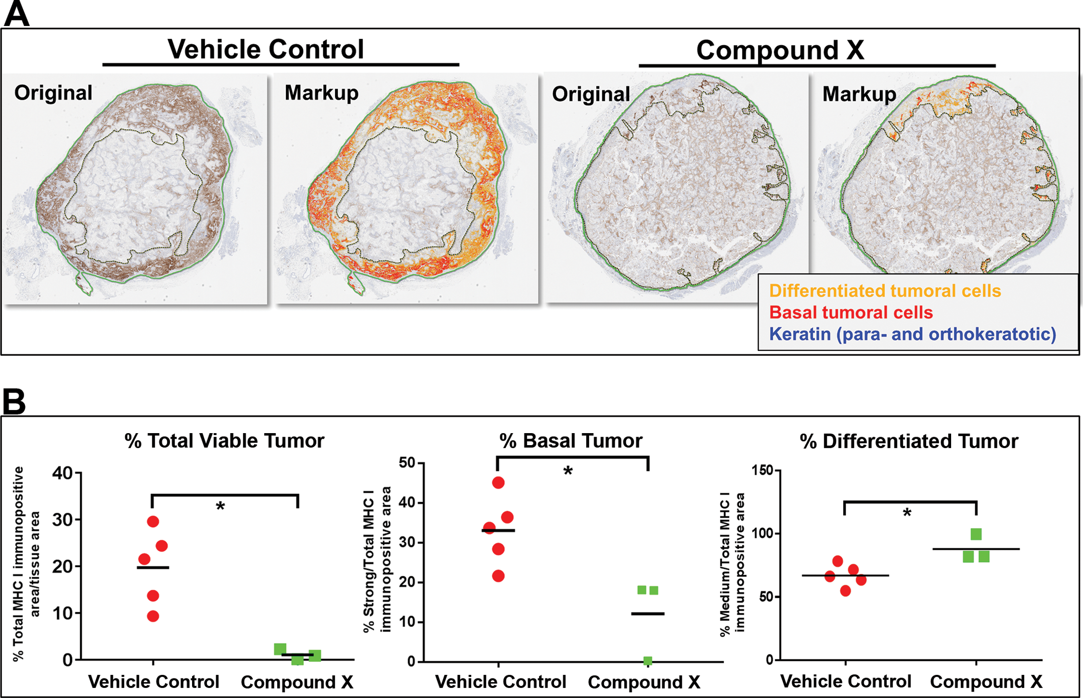
Compound X–related reduction in number of viable tumor cells was quantified by user-friendly software. Sections of tumor xenografts dosed with vehicle control or compound X were immunostained for major histocompatibility complex, class I, A (major histocompatibility complex I) to label human tumor cells. Region of interest was defined manually. Then, HALO™ area quantification algorithm was used to mark 3,3′-diaminobenzidine (brown) positive pixels. Strongly immunopositive cells were classified as basal viable cells (red in markup image), and moderately immunopositive cells were classified as differentiated tumor cells (red and orange, respectively, in markup image). The keratin debris was classified as negative. Nonspecific signals were excluded for analysis. Note that a significant compound-related decrease in percent total viable tumor cells and percent basal tumor cells. However, there was a compound-related slight increase in the number of differentiated tumor cells.
Case Study Using a Cell-based Algorithm
The IA task was to quantitate the number of proliferative (Ki67 positive) activated hepatic stellate cells (aHSCs; α-smooth muscle actin [α-SMA], positive) in human fibrotic liver and compare it with the commonly used mouse models of hepatic fibrosis. Human normal (n = 2) and fibrotic formalin-fixed paraffin-embedded (FFPE) liver sections of various etiologies, including nonalcoholic steatohepatitis, hepatitis C, unknown origin (n = 5) were dually immunostained for Ki67 (brown chromogen) and α-SMA (purple chromogen). For comparison, liver sections from commonly used mouse models of hepatic fibrosis (carbon tetrachloride [CCl4], bile duct ligation [BDL], and metabolic disease [ob/ob high-fat diet]; Delire, Starkel, and Leclercq 2015), and their respective vehicle/sham controls were also used. Whole slide quantitative IA was performed using HALO cytonuclear algorithm. Nuclei were first identified by color deconvolution, and then a cell was defined with a fixed maximum diameter, followed by detection of nuclear positive Ki67 and cytoplasmic positive α-SMA staining. The number of Ki67+, α-SMA+, and dually positive cells per unit area of the liver section was quantified. Human fibrotic/cirrhotic liver samples showed only 1.9% (range 1.3–3%) of aHSCs were positive for Ki67. In contrast, BDL, leptin deficient (ob/ob) high-fat diet, and CCl4 mouse models showed approximately 4%, 5%, and 17% of aHSCs that were positive for Ki67, respectively. In summary, cognizance of the discrepancy in the number of proliferating HSCs between human fibrotic/cirrhotic samples and mouse models of fibrosis will assist in careful design of preclinical studies. In this example, simple user-friendly software packages contributed to granular data on critical questions in translational research.
Case Study with ISH Algorithm
With the technological advancements and advent of novel sensitive assays, such as RNAscope® (Advanced Cell Diagnostics Bio, Hayward, CA), we are in a position to quantify mRNA levels in situ in FFPE samples. These technologies claim that each punctate dot signal represents a single test target mRNA molecule (https://acdbio.com/). Based on the discrete detection of mRNA signals, there are few IA software packages (e.g., HALO ISH algorithm, Definiens Tissue Studio Spot Detection algorithm) available for automated quantitation of mRNA dots. In these algorithms, the most common readout is the number of punctate dots per cell or per unit area of the tissue analysis. However, these algorithms do not clearly address the issues associated with the clustered spots/signals. Therefore, we performed investigative studies to determine the best quantitation tools and best readouts of ISH signals. Two examples were used: (1) mouse brain sections with fairly discrete spots and (2) mouse liver sections with a treatment-associated increase in the number of clumped signals. With the discrete spots, comparable results were obtained with the area quantitation and signal numbers (Figure 10A). However, spot classification was not adequate with the clustered signals (Figure 10B), and there was a discrepancy between area and signal number readouts. In summary, the pilot investigative studies concluded that mRNA stained area is a better indicator than number of mRNA spots if the signals are clumped; therefore, signal area is considered a better indication of mRNA signal quantity.
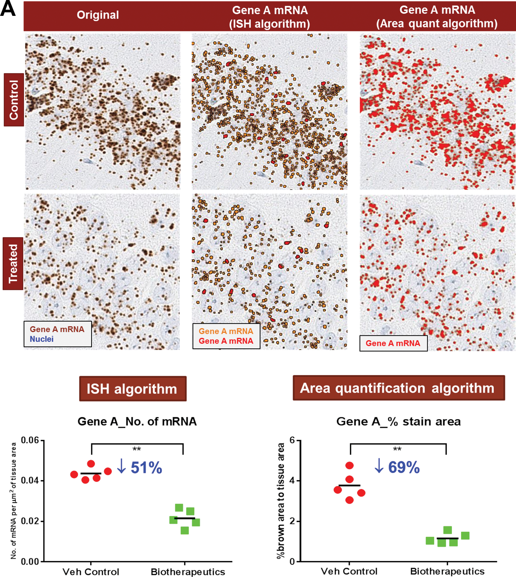
Signal area is a better indicator for quantitative in situ assessment of messenger RNA (mRNA). (A) Quantitation of in situ hybridization (ISH) signals (with fairly discrete spots) in vehicle control and biotherapeutic-treated mouse brain sections by HALO ISH, and area quantification algorithms were compared. Segmentation of brown signals as spots by ISH algorithm and as brown signal positive pixels by area quantitation algorithms was satisfactory. Note that the biotherapeutics treatment-related change in numbers mRNA spots (by ISH algorithm) was comparable to the signal area (by area quantification algorithm). (B) In another example, mouse liver sections with a treatment-related increase in the number of clumped signals were used. Note that spot classification with ISH algorithm was not adequate with the clustered signals. This is reflected in the quantitative data (graph), wherein treatment-related induction of mRNA was found to be 3-fold. On the other hand, area quantification showed an 8-fold change in the signal area in the treatment group and that agree with the pathologist evaluation.
Image Enhancement Methods to Visualize Spatial Distribution of Signals in Tissue Sections
Evaluation of pattern/spatial distribution of IHC/ISH signals or features in tissue sections at low magnification in an unbiased manner is challenging. Such evaluation requires several rounds of changing views between high and low magnification, which can be time consuming, ineffective, and often lead to loss of spatial context. Tissue IA is quite often used to quantitate signals/features in tissue sections. The algorithms supply high-level view of the ROI, but masks of ISH/IHC signals or small features require visualization at high magnification. Two case studies were discussed; wherein the masks of signals were enhanced and visualized at high magnification using either open-source image processing tools or commercially available IA algorithms. The goal of the first case study was to identify the ROI for a biotherapeutic-induced change in mRNA signals in mouse sagittal brain sections. Definiens Tissue Studio Nuclei and Spots algorithm was used to classify the mRNA spots. This image layer was then processed with Definiens Developer XD. At 40× magnification, the image layer with classified mRNA spots was segmented into smaller objects (100 × 100 pixels), and color visualization (heat map) was created based on the density of spots in each object. The heat map visualization of mRNA spot density showed regions of brain sections (e.g., hippocampus) where significant changes in mRNA levels of the gene of interest were apparent even at low magnification (1×). This study illustrated yet another value of routinely used quantitative IA tools to visualize subtle changes in mRNA signals in histologic sections of brain, thereby improving the efficiency of defining ROIs for further focused quantitative analysis. In another example, the goal was to compare the autoradiography pattern of a ligand binding to that of protein expression in tissue sections. A small molecular ligand specific for a protein (i.e., known to be expressed at high levels in diseased human lung tissues) was designed to use as an in vivo biomarker for the disease progression. To test the specificity, the radiolabeled ligand was allowed to bind to frozen lung sections, and the labeling pattern was visualized as a heat map (Figure 11). On a sequential section, IHC was performed to localize the protein of interest. To visualize the IHC signal distribution in lung sections, the signals were segmented using Definiens Tissue Studio marker area algorithm. Heat map was created based on the area of the signal in subsets of image analyzed. The mask images from Definiens were postprocessed by image processing libraries in Python, wherein binary images were generated followed by dilation of pixels and inversion of the images. Heat map (based on area) or enhanced visualization of IHC signals at low magnification did not correlate to the ligand binding pattern on tissue sections as shown by autoradiography (Figure 11).
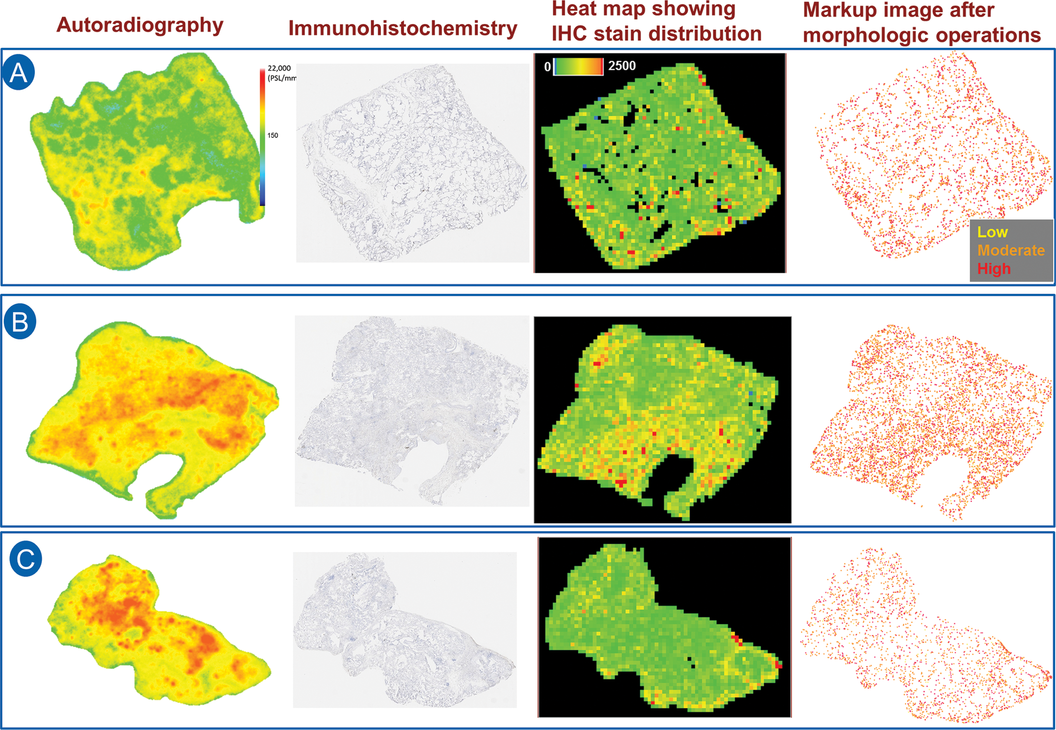
Image enhancement methods to visualize spatial distribution of signals in tissue sections. Radiolabeled small molecule ligand (i.e., known to be expressed at high levels in diseased human lung) was allowed to bind to normal (A) and diseased lung sections (B, C). Autoradiography of the ligand binding was represented as a heat map (column 1). To test the specificity of the ligand, the protein expression by immunohistochemistry (IHC) in the serial lung sections was evaluated. But the signal distribution was not appreciable at high level (low magnification; column 2). Therefore, image enhancement methods were used to show the distribution of signals. Heat map representation of the IHC stain area was developed by Definiens Tissue Studio® (column 3). In addition, mathematical morphologic processing (binary conversion, pixel dilation, and inversion) was performed by Python-based open-source software packages (column 4). Note that heat map (based on area) or enhanced visualization of signals of IHC signals at low magnification did not correlate to the ligand binding pattern on tissue sections as shown by autoradiography.
In summary, with the advent of newer user-friendly software packages, investigative pathologists are in a position to perform tissue IA on their own without spending much time learning the software (languages). Case studies presented were good examples of simple and common IA problems that can be solved by a pathologist. Pathologists may seek experts (engineers) if the IA questions are more sophisticated, requiring use of supervised (sophisticated) software.
Reducing Bias in IA by Applying Stereological Principles
Although IA can provide valuable quantitative information about histologic tissue sections, the results may be highly biased (inaccurate) due to multiple assumptions that are made about the tissue sections being evaluated. These include assuming homogeneity throughout the organ or ROI, assuming the sections being evaluated are representative of the tissue as a whole, assuming there is no change in organ size or volume during tissue processing, and assuming control and treated tissue respond equally to tissue shrinkage. Many of these biases can be minimized by employing stereological principles to IA studies. This presentation by Dr. Danielle Brown (Charles River Laboratories, Durham, NC) focused on bringing to light the potential biases introduced by 2-dimensional (2-D) morphometric analysis and how to implement stereological principles to minimize those biases when possible
In IA studies, the most optimum tissue sections are often analyzed. These are nonrandom and introduce sampling bias, meaning some of the objects within the population are less likely to be included in the sample than others. This is particularly troublesome in tissues that are very inhomogeneous such as the brain. Sampling bias can also occur when the microscopic fields of view for analysis are chosen. If these fields are chosen “randomly” by the scientist, the issue of user bias comes into play when choosing those fields. In the true sense, statistical analysis of intergroup differences is not valid when sampling bias exists because statistical methods for hypothesis testing always presume that there is random sampling (Boyce, Boyce, and Gundersen 2010; James 1989).
One way to minimize sampling bias is to apply the stereological principle of SURS. This is a stereological sampling principle that ensures every structure has an equal probability of being sampled. To accomplish this, the organ or ROI is sectioned at regular intervals (T) with the first interval randomized (Figure 12). In stereology, the rule of thumb is to section at an interval that will yield approximately 8 to 10 sections through the tissue or ROI. For small tissues, SURS can be accomplished entirely at microtomy through the use of an automated microtome with a calibrated microtome advance. For medium-sized tissues, such as rat heart or nonhuman primate pancreas, the entire tissue can be processed and embedded in paraffin and sectioned into slabs for analysis (Brown 2017b). If paraffin-induced shrinkage is undesirable (e.g., if volume estimates are an important end point), the tissue can be embedded in agar and sectioned into slabs by SURS using a tissue slicer or matrix, then processed and embedded in plastic (Brown 2017b). For larger tissues, SURS may need to be performed in several subsampling steps, which may be unique for each organ or tissue type (Gundersen et al. 2013). SURS can also be applied during microscopic field selection by the software system if whole slide imaging is utilized. The user can select a percentage of the tissue to analyze, and the computer can choose the first field randomly and subsequent fields regularly spaced across the tissue or ROI (Figure 13).
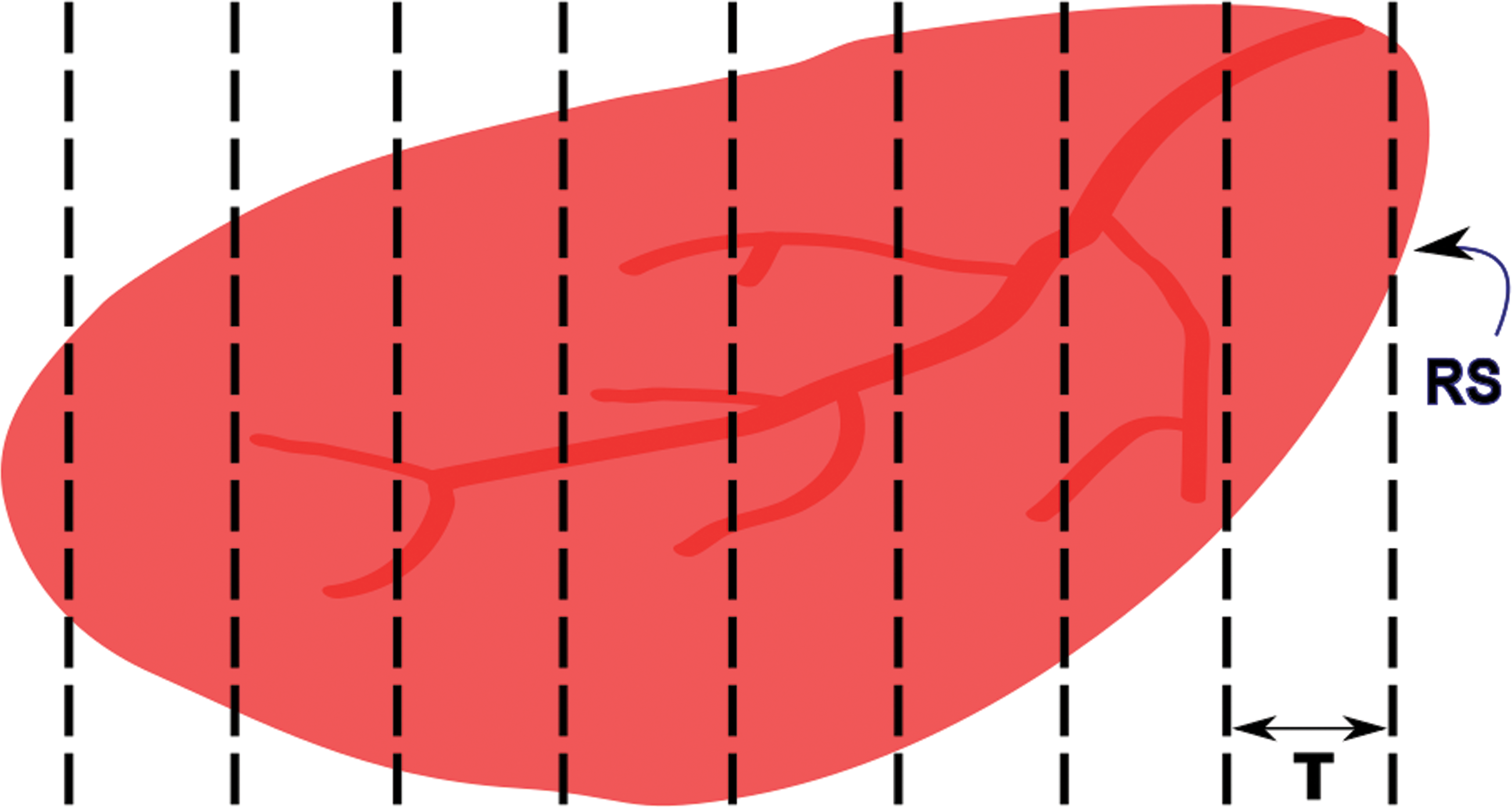
Systematic uniform random sampling of an organ. The length of the tissue is measured, and the distance between sections (T) needed to obtain 8 to 10 sections through the tissue is calculated. The first section is obtained at a random start of 0 to T, and subsequent sections are taken at regular intervals of T.
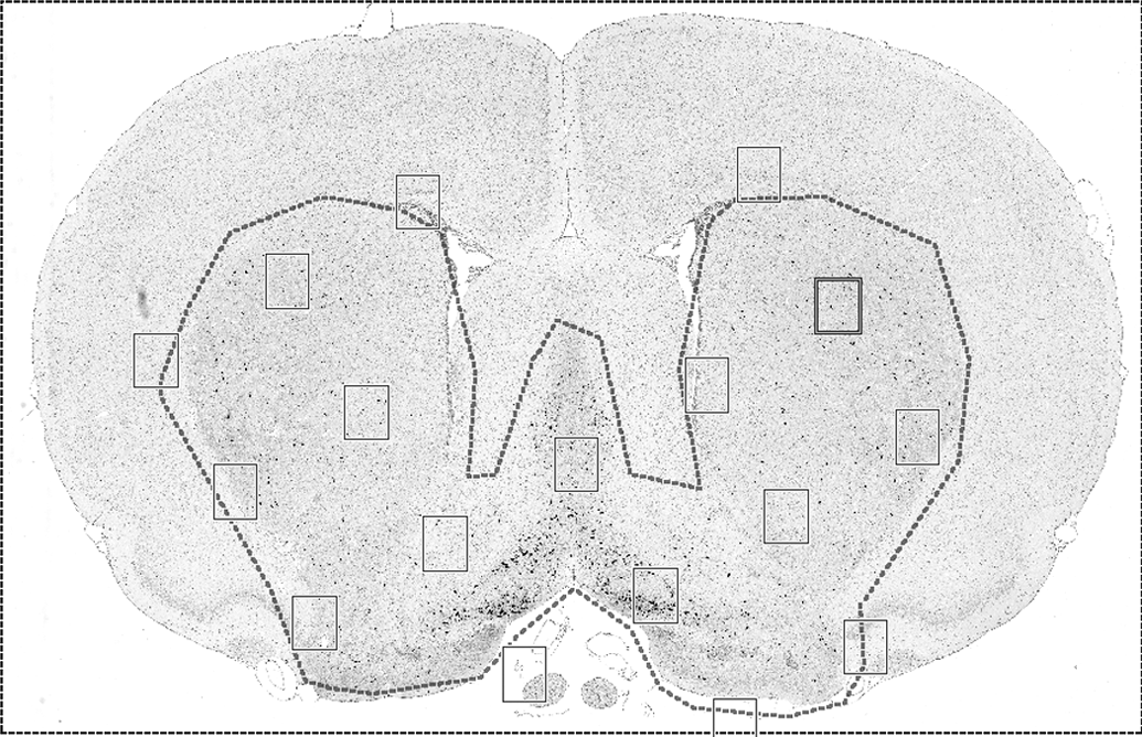
Systematic uniform random sampling of microscopic fields of view for analysis. The user defines a region of interest (ROI; basal forebrain in this example) and selects a percentage of the ROI for sampling (i.e., 20%). The computer then selects the first field randomly and subsequent fields at regularly spaced intervals across the ROI. Rat brain stained for choline acetyltransferase.
For objects that have nonrandom orientation within the tissue section, such as capillaries, larger blood vessels, nerve fibers, and bone trabeculae, it may be important to eliminate directional bias when sampling the tissue. This can be accomplished through obtaining isotropic uniform random sections. Isotropy ensures that all directions have an equal chance of being chosen. Two methods for obtaining isotropy are the orientator and isector techniques (Howard and Reed 2005; Mattfeldt et al. 1990; Nyengaard and Gundersen 2006; Nyengaard and Bendtsen 1992). With the orientator technique, the tissue is embedded in agar, and the agar outside of the tissue is sectioned at a random angle using an equiangular clock. The cut side is placed down on a cosine-weighted clock, and the agar is cut at another random angle. This cut side is then placed against the end of a tissue slicer, and slabs are cut through the tissue (e.g., see Brown 2017b). With the isector technique, small pieces of tissue are placed into spherical molds, which are filled with agar and left to harden. The hardened spheres are rolled on a table to obtain a randomized orientation, and the tissue is embedded in the desired embedding medium. In some cases, it may be desired to have uniform orientation of objects between tissue samples rather than randomized orientation when IA is being performed. The important thing is to consider these potential biases early in the study design process and to modify the study procedures to best fit the desired end points.
What if the tissue has already been sectioned and IA is to be applied retrospectively? In some cases, all that are available are the tissue blocks and SURS cannot be applied to the tissue as a whole. In these retrospective studies, it is still important to analyze multiple sections through the tissue in order to obtain a representative sample. Several sections can be taken through each block, spaced far enough apart as to not analyze the same objects or areas more than once. The first section can be randomized.
It is known that tissue processing, paraffin processing in particular, introduces substantial tissue shrinkage. Previous studies looking at kidney tissue have shown 15–40% reduction in size/volume estimates following paraffin processing (Iwadare et al. 1984; Miller and Meyer 1990). When final estimates are expressed as densities or ratios, such as occurs with 2-D IA, increased tissue shrinkage results in overestimation of number and underestimation of volume. This issue may be magnified if control and treated tissue respond differently to the processing-induced shrinkage. Because the ratios/densities obtained with IA are often irrespective of processing- or treatment-induced changes in the tissue as a whole (reference space), it is difficult to impossible to extrapolate the density/ratio values to absolute values, a problem commonly referred to as the “reference trap.”
Bias introduced by the reference trap can be minimized through measuring the reference space and calculating the amount of processing-induced shrinkage in each tissue. The volume of the tissue can be determined at necropsy by Archimedes’ principle, in which the tissue is placed into a glass container of water or another isotonic solution of a known density and the weight change of the container is noted (Scherle 1970). Alternatively, Cavalieri’s principle can be used to estimate the volume of the reference space (Howard and Reed 2005). Following tissue processing and sectioning into slabs, a point grid is overlain on the tissue slabs (subgross level), and the number of points intersecting the tissue is counted and summed. The volume is then calculated as the number of points “hitting” the tissue (reference space) multiplied by the distance between the sections (T) and the area per point (cross-sectional area between points on the grid; Figure 14). If whole slide imaging is being utilized, the cross-sectional area of each tissue section can also be calculated and used and multiplied by T to obtain the total tissue volume. Cavalieri’s principle is a better indicator of the reference space at the time of IA in that it is calculated postprocessing and takes into account processing-induced tissue shrinkage. Bias from the reference trap can also be minimized by estimating the degree of processing-induced shrinkage for each tissue. This can be accomplished simply by weighing the tissue pre- and postprocessing and calculating the global shrinkage using the following equation: shrinkage = 1 − W post / W pre, where W pre is the preprocessing weight and W post is the postprocessing weight (Gundersen et al. 2013). Statistical analysis can then be used to determine whether there are intergroup differences in processing-induced shrinkage.
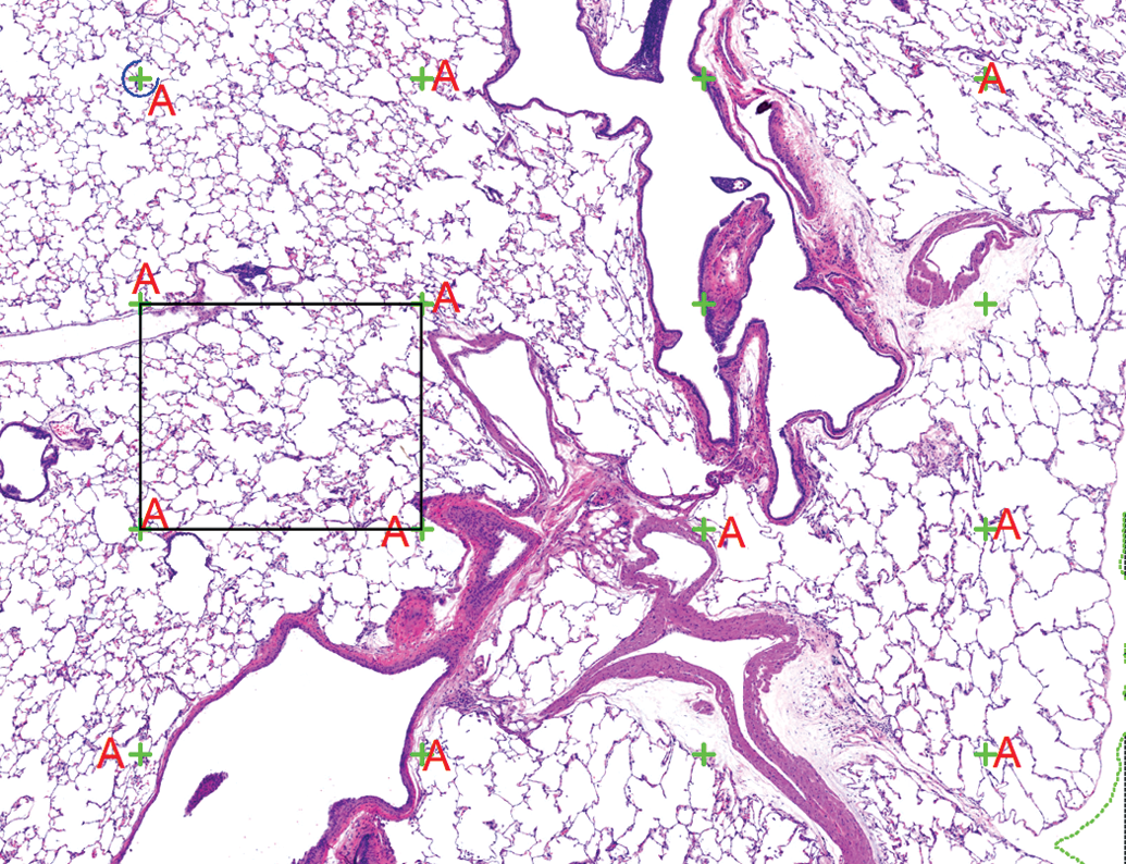
Estimation of total tissue volume using Cavalieri’s principle. A point grid (green crosses) is placed over the tissue at a low magnification (original objective 4× in this example), and the points that intersect the pulmonary parenchyma are tagged (A). Note that the points intersecting large blood vessels and large airways were not included in this analysis. The total volume is calculated by multiplying the sum of the tagged points by the distance between the sections (T in Figure 12) and the area per point (cross-sectional area of the black box). Rat lung, hematoxylin, and eosin stain.
There is at least one instance in which bias really cannot be minimized in 2-D analysis; geometrical bias. When a 2-D histological section is taken through a 3-D tissue, all of the information about the size, shape, and orientation of the objects within that tissue is lost. Therefore, there is no mathematical relationship between the number of profiles in 2-D and the number of objects in 3-D. Objects are counted according to their size and orientation rather than their number, as larger or perpendicularly oriented objects are more likely to be counted. This is particularly problematic with objects that are not uniform in size, shape, and orientation, such as alveoli within the lung. The consequences of this bias range from overestimation of cell number to a treatment effect that is in the opposite direction of the truth (Brown 2017a). Correction factors, such as the Floderus or Abercrombie methods, are applied to 2-D data and claim to correct for the geometrical bias; however, these methods are all based on assumptions in and of themselves, leading to additional bias (West 1996). Studies have shown that application of these correction factors can contribute to inaccuracy of the data (Mendis-Handagama and Ewing 1990; Pakkenberg et al. 1991). In order to estimate cell or object number unbiasedly, the stereological principle of the disector needs to be applied. With this method, a volumetric probe (either consecutive sections, also known as the physical disector; or thick sections, also known as the optical disector) is applied at each sampling interval. This method ensures that cells are sampled according to their number rather than according to their size, shape, or orientation (Sterio 1984; Gundersen et al. 1988). Because of the bias introduced by 2-D methods, several professional societies and high-profile journals have issued position papers and statements on the use of 2-D methods for quantifying objects, particularly number estimation (Huisman et al. 2010; Madsen 1999; Saper 1996).
In summary, IA provides interesting and valuable information about tissue sections at a higher sensitivity than the human eye alone can accomplish. However, the data can be highly biased due to several assumptions that are made about the tissue. Sampling bias can be minimized by applying the stereological principle of SURS, both at the tissue sampling level and when microscopic fields of view are chosen for analysis. Bias introduced by the reference trap can be minimized by estimating the total tissue volume and the amount of processing-induced shrinkage. There is no way to eliminate geometrical bias with 2-D analysis; therefore, stereological methods such as the disector need to be applied to accurately count cells or objects.
Concluding Remarks
Recent technological advances in automated whole slide digitizer systems, innovative, and increasingly pathologist-friendly IA platforms provide confidence that the technology exists to support pathologists in strengthening their medical diagnoses with quantitative assessments, thereby adding value to preclinical investigations. Pathologists need to carefully assess their needs based upon their field of expertise and promptly integrate these new tools in their daily assessments. A constant, complete, and thorough attention is required in the applications of these technologies, from experimental design, to pre-analytical steps and quantitative data generation and analysis, to ensure the data generated are relevant, meaningful, and provide further clarity to the interpretation. Further progress and example generation is needed to seek regulatory acceptance of digital pathology as a “gold standard” preclinical end point for risk assessment.
Footnotes
Acknowledgments
The authors would like to thank Corinne Berclaz (Roche pRED, Basel, Switzerland) for scientific expertise related to digital pathology workflows, Julie Boisclair (Novartis Institutes for Biomedical Research, Basel, Switzerland) for providing case studies, and Cynthia Swanson (Charles River Laboratories, Durham, NC) for assistance with images.
Author Contribution
All authors (RD, VS, CS, DB, JG, MO, MS) contributed to conception or design; data acquisition, analysis, or interpretation; drafting the manuscript; and critically revising the manuscript. All authors gave final approval and agreed to be accountable for all aspects of work in ensuring that questions relating to the accuracy or integrity of any part of the work are appropriately investigated and resolved.
Declaration of Conflicting Interests
The author(s) declared no potential conflicts of interest with respect to the research, authorship, and/or publication of this article.
Funding
The author(s) received no financial support for the research, authorship, and/or publication of this article.