Design-based Stereology

Abstract

In regulatory toxicology studies, qualitative histopathological evaluation is the reference standard for assessment of test article–related morphological changes. In certain cases, quantitative analysis may be required to detect more subtle morphological changes, such as small changes in cell number. When the detection of subtle test article–related morphological changes is critical to the decision-making process, sensitive quantitative methods are needed. Design-based stereology provides the tools for obtaining accurate, precise quantitative structural data from tissue sections. These tools have the sensitivity necessary to detect small changes by combining statistical sampling principles with geometric analysis of the tissue microstructure. It differs from other morphometric methods based on tissue section analysis by providing estimates that are statistically valid, truly three-dimensional, and referent to the entire organ. Further, because the precision of the stereological analysis procedure can be predicted, studies can be designed and powered to detect subtle, potentially toxicologically significant changes. Although stereological methods have not been widely applied in toxicologic pathology, recent advances have made it feasible to implement these methods in a regulatory toxicology setting, particularly methods for estimation of total cell number.

Introduction

The toxicologic pathologist plays a major role in defining test article–related effects that include hazard identification and determination of a NOEL/NOAEL for a given test article, and, via risk assessment, determination of safe levels for humans. In regulatory toxicology studies, the qualitative/semiquantitative histopathological evaluation by an experienced pathologist meets regulatory needs in the majority of cases. However, in certain settings, it may not have the sensitivity necessary to detect potential subtle tissue structural changes such as small changes in cell number. When quantification of subtle structural changes from histological sections is needed to detect potentially adverse, irreversible, or unmonitorable test article–related effects, sensitive, accurate, and precise quantitative methods are required. Historically, quantitative methods generally referred to as two-dimensional (2-D) methods have frequently been employed to address such issues, for instance, cell profile density counts on sections collected for routine histopathology. However, these 2-D methods have limitations. Two-dimensional methods make assumptions about the organ, tissue, or structure of interest and generate data based on surrogates of three-dimenstional (3-D) tissue structure (e.g., cell profile counts as a surrogate of cell number) and do not report quantitative data referent to the whole organ. These inherent assumptions not only limit sensitivity and confound statistical accuracy, they are associated with a high risk of both Type I and Type II errors. The limitations of 2-D methods can be avoided through the use of sensitive methods broadly known as design-based stereology. Stereological methods offer practical and scientifically valid approaches for obtaining accurate, precise quantitative estimates of subtle structural changes in tissues from histological sections. The data from stereological analyses convey changes in the true 3-D tissue structure at the whole-organ level. In contrast to traditional 2-D methods, design-based stereological methods rely on statistical sampling principles and stochastic geometric theory to estimate quantitative parameters of 3-D geometric objects such as complex tissue structures. The statistical and mathematical principles used in stereology guarantee that no assumptions—or bias—are introduced in the analysis. Stereological methods have evolved from being cumbersome and time-consuming to being efficient and practical because of combined advances in stereological theory, sampling techniques, software, and imaging devices. With sufficient technical and capital resources, design-based stereological protocols are amenable to implementation in a regulatory toxicological setting, particularly when estimation of cell number is an issue.

The objective of this review is to provide an introduction to design-based stereology that includes discussions of basic principles, value of the methodology, and use in toxicologic pathology practice. Following this introduction, the review then focuses on specific methods for analysis of cell number, a frequent quantitative endpoint in toxicologic pathology, and addresses the pitfalls of using profile counts on routine sections collected for histopathology.

Basic Principles of Design-based Stereology

To appreciate what stereology is and its value, it is important to first consider the consequences of sectioning tissues into histological sections. Tissues are, in essence, a composite of complex geometric structures that occupy 3-D space, each with associated length, width, and height. When this composite of complex geometric structures is sectioned with a microtome, it is essentially equivalent to introducing a series of 2-D planes into the complex structure. The introduction of a 2-D plane effectively reduces 3-D structures to a series of 2-D profiles in the section plane (Figure 1). Dissimilar 3-D structures can produce similar 2-D profiles, and similar 3-D structures can produce dissimilar 2-D profiles. Additionally, the position and orientation of the sectioning plane will influence size, shape, and frequency of these 2-D profiles. The pathologist has learned to evaluate these profiles and conceptualize 3-D relationships. However, the restoration or reconstruction of the 3-D structural information from histological sections is not simple. Serial reconstruction using thin sections or optical sections collected with a confocal microscope is an elegant but rather labor-intensive technique to obtain quantitative information about 3-D structures; a more efficient approach is design-based stereology.

Figure 1.

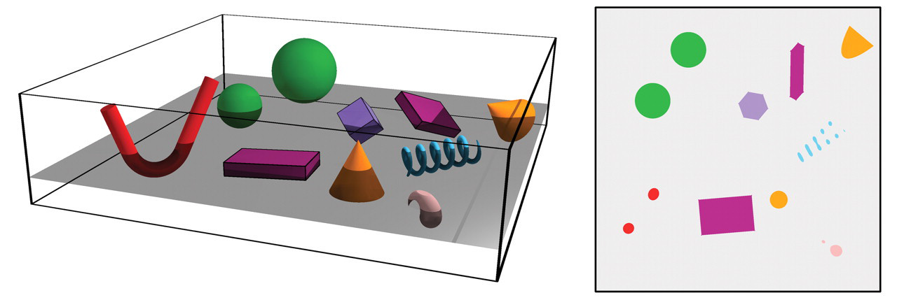
Sectioning a complex 3-D structure with a sectioning plane results in loss of 3-D information, as 3-D structures are reduced to 2-D profiles in the section plane. Dissimilar structures can produce similar profiles and vice versa.

Stereology is a mathematical science based in statistics and stochastic geometry. Stereology provides efficient tools for estimation of geometric quantities such as volume, surface area, length, or number of objects for 3-D tissue structures contained within an organ from measurements made on a set of 2-D sections. Stereological analyses involve a two-step process. Statistical sampling principles are used to obtain statistically valid histological sections from an organ to reduce the amount of tissue for analysis without reducing the precision of the estimate. Then, appropriate geometric probes (e.g., points, lines) are superimposed on sections and the number of interactions of the probes with the structural feature being estimated is determined. This count, unlike surrogate 2-D parameters, has a known mathematical relationship to the structural quantity in 3-D tissue space. The statistical sampling principles used in stereology guarantee that no bias is introduced in choosing sections or microscopic fields for analysis. The mathematical basis of the geometric probes ensures the three-dimensionality of the measurements. These collective principles are the basis for the enhanced sensitivity of these methods. In the context of Good Laboratory Practices, it is important to note that stereological principles are not verified or validated by experimental data but rather by mathematical proofs, similar to other statistical principles.

A scientific strength of design-based stereology is that, if performed properly, it guarantees accurate (unbiased) and precise quantitative estimates of tissue structure in an efficient manner. This statement may seem dogmatic for those less familiar with the statistical concept of accuracy or unbiasedness. In statistics, accurate (unbiased) methods yield estimates that, on average, converge to the true population mean with replication. Thus, replication of an unbiased estimate increases the precision or reproducibility of the mean estimate. In contrast, biased or assumption-based methods yield estimates that do not converge to the true population mean—that is, biased estimates become, on average, more precisely inaccurate with replication (Figure 2). The deviation from the true value is the systematic error or bias that cannot be sensed or detected unless the true population value is known (rarely the case in biology).

Figure 2.

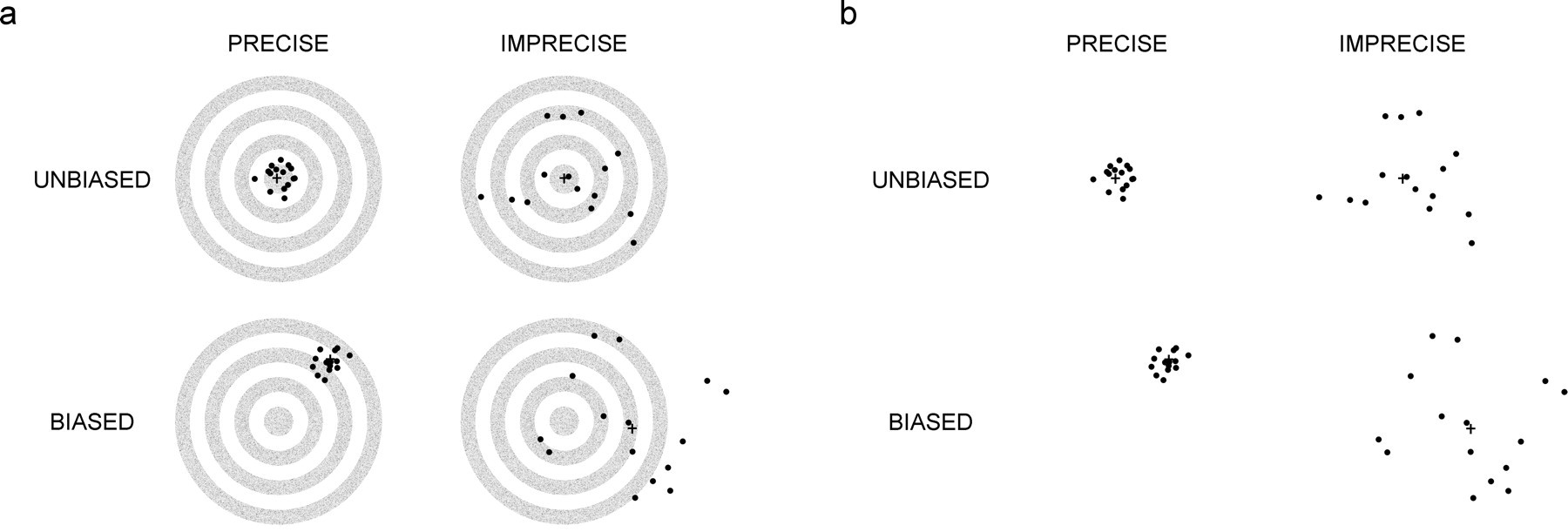
Simplified illustration of the statistical concepts of accuracy, unbiasedness, and precision. In Figure 2a, the targets in the top row depict the statistical consequences of application of unbiased methods that guarantee the mean value, indicated by the cross-hatch, on average, estimates the true population value. The true population value is located within the “bull’s eye” of the target. The data may have low variance and be very precise (left target), or they may have higher variance (right target). The statistical consequences of biased methods are depicted in the lower row of targets. Data may be either very precise (left target) or highly variable (right target), however, the mean value for biased estimates regardless of the variance, on average, will never converge to the true population value, that is, the mean value never hits the “bull’s eye.” Figure 2b is a duplication of Figure 2a that depicts real life, where the population mean is unknown and there is no “bull’s eye” to inform the researcher if data are biased. Modified from Figure 2 in Gundersen (1992).

Efficiency in the context of design-based stereology is a key consideration. Efficiency should be understood to reflect the number of samples and counts of interaction with geometric probes necessary to obtain a precise estimate. Precise estimates can be obtained with relatively few measurements made on a small number of sections, typically between 100 and 200 “counts” in fifty microscopic fields sampled from six to ten sections. Theoretical advances in design-based stereology over the past twenty years have focused on efficiency with development of methods that give the most precise estimates with the least amount of work.

There are, however, specific requirements with respect to the sections and measurements that must be met in order for the estimates to be accurate. To understand these specific requirements, it is useful to consider opinion polling and stereology as analogous sciences (Textbox 1), as suggested by Adrian Baddeley, a renowned stereologist and statistician (Baddeley 1993). Both sciences use similar statistical principles to guarantee accuracy of results. The first requirement to ensure an accurate opinion poll is that a representative sample of the entire population must be obtained. The simplest way to obtain a representative sample is to use sampling methods that ensure all people in the population equal probability of being sampled; these sampling methods are known as uniform random sampling. Uniform random sampling is basically random sampling as known to most biologists. The second requirement is that the representative sample of the population is questioned or “probed” in such a way to avoid influencing or biasing the response—to make certain the response reflects the truth. The reproducibility or precision of the opinion poll, conveyed as the sampling error, can be improved by sampling more people and can be reliably predicted based on the number of people sampled. By analogy, stereology is a 3-D opinion poll of an organ. It shares the requirements for a representative sample and unbiased “probing” to ensure accuracy of the estimate, and like opinion polling, the precision of the estimate can be improved with increased sampling. Although adherence to stereological principles guarantees unbiased estimates, rigorous attention to aspects of the technical implementation of these principles at each step of the analysis is required to avoid introducing bias. Potentially confounding technical issues include but are not limited to tissue processing-induced shrinkage, inconsistent sectioning, and inadequate staining.

Textbox 1. Principles of design-based stereology are similar to population statistics

Just as a pollster may poll a small sample of people to estimate the outcome of an election, a pathologist may count hepatocytes immunolabeled with a proliferation marker in a small sample of liver to assess the risk of hepatic carcinogenesis. The accuracy and precision of the estimate determines the probable success of either process. Accuracy of the poll or the estimate of immunolabeled hepatocytes can be ensured by strictly adhering to sampling protocols that are mathematically proven to provide results that on average equal the true population value. The accuracy of the poll can be judged retrospectively because the true population value will be shown by the actual outcome of the election. For biological systems, there is rarely any way to judge the accuracy of quantitative estimates, because the true population value is rarely known. Fortunately, the statistical principles used guarantee accuracy without knowledge of the true population value.

There are two requirements that must be met in both polling and stereology to guarantee accuracy of results. The first requirement is that a representative sample must be obtained from the entire population. The pollster might like to poll well-dressed professionals in urban areas and the pathologist may have a strong preference for working with optimum sections taken from the center of one or two defined liver lobes, but neither approach will yield an accurate estimate. A representative sample of the population is one that is prospectively designed to give every person or every immunolabeled hepatocyte in the liver—regardless of size, shape, distribution, or spatial orientation—an opportunity or probability of being polled or counted. Obtaining a representative sample therefore requires the entire population or region of interest to be available for sampling and is sampled with known probabilities (most often, equal probability using uniform random sampling). Any deviation from this sampling principle will result in systematic error or bias, which directly abrogates the guarantee that the results are accurate.

The second requirement is that the representative sample is questioned, or “probed,” in a way that avoids influencing or biasing the response. If the questionnaire used in an opinion poll favors a certain response, there will be systematic error or bias, and the results will be inaccurate. Similarly, the pathologist would bias an estimate by counting profiles of immunolabeled hepatocytes in a thin histological section, unaware that cell size directly influences the probability that a cell will be counted in a section and unaware that cell size may have been imperceptibly altered by test article treatment. Hence, estimating cell number by this method would favor larger cells and bias the estimate. The geometric probes of stereology (the sets of points and lines, and so on), like the questionnaire of the pollster, are the tools used to “probe” or question the sampled tissue structures in the correct way not to favor the response, thus ensuring an accurate result.

Obtaining Representative Samples in Stereology

The first requirement for obtaining a uniform random sample from an organ is that the entire organ must be available for sampling. This requirement may be a major hurdle in regulatory toxicology, because issues often arise after studies have been completed. However, it is a requirement that must be met, necessitating either prospective inclusion of appropriate sampling at necropsy or additional studies.

Stereologists generally sample an organ using a form of random sampling known as systematic uniform random sampling (SURS). Figure 3 compares SURS with simple uniform random sampling in a hypothetical organ. With simple uniform random sampling, all sampling positions are chosen at random, for example, with the aid of a random number table to select sampling locations using a ruler positioned beside the organ. Although the sampling is uniformly random—giving all positions equal probability of being sampled—it will take many sections to reach a satisfactory level of precision for an estimate of a quantity of a geometric feature such as total volume of pancreatic islets sampled by those sections. The distribution of the structure of interest throughout the organ contributes to section-to-section variation, and this variation influences the number of sections needed to reach a certain level of precision. With SURS, the organ is sliced at regular uniform intervals (T), but the first cut is positioned randomly within the first interval (0-T) by using a random number table to select the position in 0-T. The latter step constitutes the random element of the sampling. This sampling method ensures all positions in the organ are given equal probability of being sampled and is essentially always more efficient than simple random sampling (Gundersen and Jensen 1987). Systematic uniform random sampling is better at capturing variation because it samples uniformly and regularly across an organ.

Figure 3.

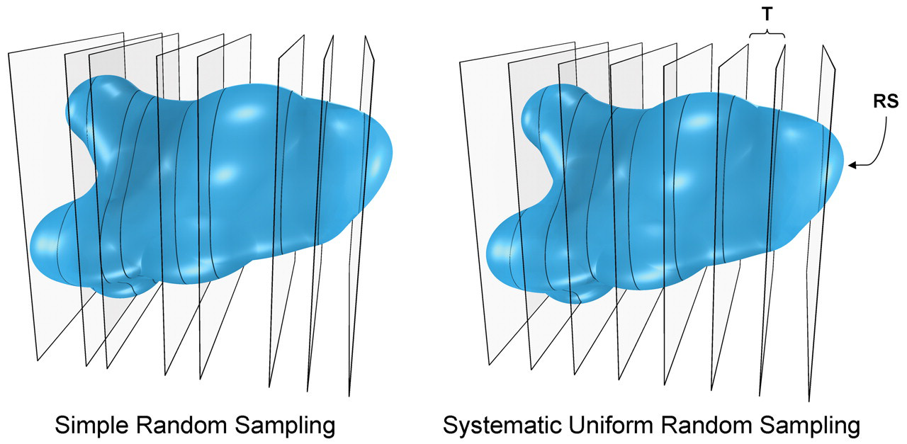
Simple uniform random versus systematic uniform sampling of a structure. Simple uniform random sampling is depicted in the left figure, where the structure is cut at independent random positions along its longitudinal axis. Systematic uniform random sampling is depicted on the right. The structure is cut at a uniform constant interval (T) with a random start (RS), that is, the first cut is positioned uniformly random in the interval 0 to T, selected from a random number table or from randomly positioning of the organ in an agar block prior to sampling.

Once an organ is cut into slabs, additional subsampling using SURS can further reduce the amount of tissue to be analyzed (Figure 4). Sampled organ slabs can be cut into bars and sampled, and then sampled bars can be cut into cubes. Sampled cubes are embedded and sectioned, yielding a set of statistically representative sections for analysis. Microscopic fields are then sampled by SURS for probing with the appropriate geometric probe to estimate the quantity of a geometric feature of interest.

Figure 4.

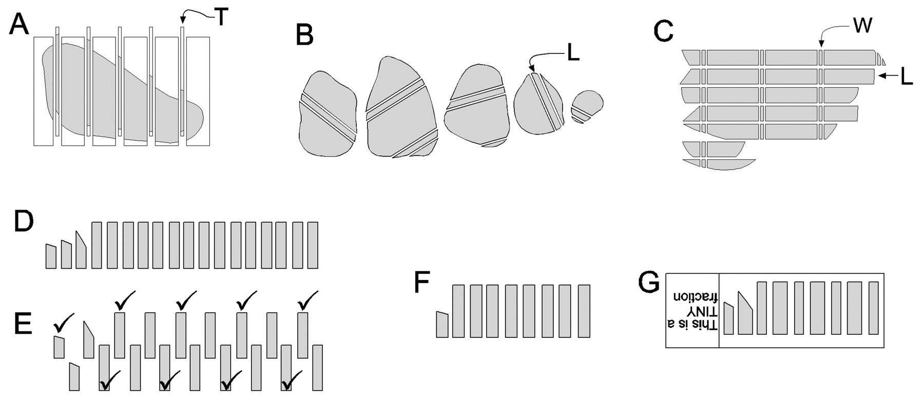
Subsampling schema for a large organ to reduce sample size for analysis. (A) The organ is embedded in agar in a cutting device, and a set of systematic uniform random (SUR) slabs of thickness T are prepared. (B) A set of SUR strips of width L are then cut. (C) Strips are aligned and a set of cubes are prepared at SUR locations of width W. (D-F) Cubes are then sampled using the smooth fractionator, a sampling method that reduces variance between subsamples collected from an organ (Gundersen 2002). (D) Cubes are arranged by increasing size, then (E) every other cube is pulled down to create a second row. Cube size ascends moving left to right on the top row, then descends moving right to left on the bottom row. Every second cube is selected, moving left to right on the top row and continuing right to left on the second row as indicated by the checkmarks. The first or second cube was selected randomly by a toss of a coin. (F) The final sample is processed in a single block. (G) Section of sampled cubes where microscopic fields will be sampled for probing using SURS.

Stereological sampling principles ensure the structures of interest in an organ are sampled with equal or known probabilities, the first requirement to guarantee an accurate estimate. The concept of statistical accuracy that is guaranteed by stereological sampling is further explained in Figure 5 using SURS as an example. Stereologists have continued to develop newer and more efficient sampling methods that dramatically reduce the amount of work—or how many slabs, blocks, sections, fields, counts are needed—to achieve a precise estimate (Textbox 2).

Figure 5.

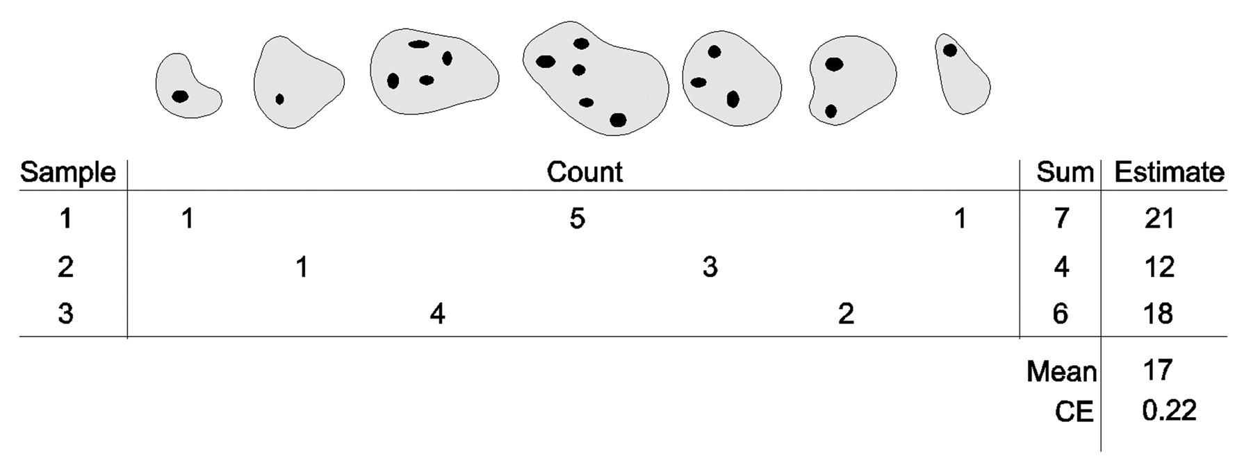
Accuracy of systematic uniform random sampling (SURS). Samples are taken from a complete set of seven sections, and cells are counted using an unbiased method (disector sampled). The entire cell population consists of seventeen cells. It is decided to take a sample of about two sections. After surveying the size of the set, it is then decided to sample every third section, that is, the sampling fraction is sf = 1/3. Systematic uniform random sampling is performed with a random start in the sampling period of 3 (the reciprocal of sf), and the random start (looked up in a random number table) can thus only be 1, 2, or 3. The three possible samples (which have identical probabilities) are shown together with the cell count they provide. The estimate is Estimate = (1/sf)×Sum. Systematic uniform random sampling is an unbiased sampling technique because the mean of all possible estimates is identical to the population total. Note that in the above list of all possible samples, each section of the complete set is represented exactly once. Note also that not one of the three unbiased estimates of 21, 12, or 18 is absolutely correct—so that is not what unbiased means. The coefficient of error (CE, see later in the text) indicates that great precision should not be expected from a sample of about two sections.

Textbox 2. Advanced sampling methods to increase efficiency

The “Fast” Fractionator is a novel, rapid sampling method for large, solid organs of which a known fraction of an intact organ is collected using cylindrical knives. The method avoids time-intensive subsampling steps at necropsy and allows for collection of multiple complete samples, including standard tissue samples for routine histopathology (Mirabile et al. in preparation).

The Smooth Fractionator is a very efficient method for subsampling of tissue (Gundersen 2002). An initial sample of tissue pieces is sorted from smallest to largest, and every second piece in the new arrangement is”pushed down” to create a new,”bell-shaped,” symmetrical arrangement of tissue pieces—small to large to small (Figure 4). Subsampling of tissue pieces is performed from this symmetrical arrangement selecting, for example, every other piece (with a random start among the first two pieces). This sampling principle allows for subsampling, which significantly reduces the amount of tissue for analysis without compromising the accuracy or precision of the final estimates.

The Proportionator is a recent estimator that combines the power of image analysis with stereology to greatly increase the efficiency of subsampling of histological sections (Gardi et al. 2008a; Gardi et al. 2008b). This method uses nonuniform random sampling (Dorph-Petersen et al. 2000) guided by image analysis–detected features of interest in the stained sections. The feature could be, for example, positive immunohistochemical staining. Simplified, all possible sampling fields are assigned a value for the image feature and subsampled based on a mathematical relationship with the assigned value. This unbiased method can increase the sampling efficiency up to twenty-five–fold compared with SURS. Proportionator sampling can be applied to both thin and thick sections—and for all estimators of structural quantities—stereological or not. Currently, the sampling method is implemented in only one commercially available software package (Proportionator^™, Visiopharm, Hørsholm, Denmark). Proportionator sampling requires optimized staining protocols that allow for conclusive pixel classification. At the time of writing, the software does not provide for detailed monitoring of the implementation. As a consequence, the Proportionator estimates should be compared to estimates obtained with fractionator sampling in a subset of samples to achieve proper function of the image analysis configuration.

Unbiased “Questioning” in Stereology: Geometric Probes

By analogy to opinion polling, the “questioning” in stereology—or asking how much geometric feature (volume, surface area, length, or number of objects) of a tissue structure is represented in the section—is done by geometric probes. Each geometric structural feature has an associated geometric probe that must be used in order to accurately estimate the quantity of geometric feature in 3-D tissue space. Geometric probes question the tissue section in a way to get a truthful response.

Figure 6 shows the relationship between geometric probes and the corresponding geometric structural feature. Probes and geometric features each have dimensions ranging from 0 to 3. The sum of the dimensions of the probe and geometric structure must equal at least 3. The basis for this dimensionality rule is derived from the geometric principle that a probe (e.g., point, line) interacts with a specific geometric structural feature in 3-D space; that geometric feature is known as its 3-D complement (e.g., volume, surface area). In essence, the dimension of the 3-D complement takes up the remaining dimensions not used by the probe. As an example, a line probe has a dimension of 1; therefore, its 3-D complement has to have a dimension of 2 (i.e., surface area). This relationship ensures the 3-dimensionality of the estimate, namely, that it is estimating or “sensing” what exists in 3-D tissue space (see third row of Figure 6). If the sums of these dimensions equal 3, the interaction of the probe with the structure is a simple, countable event. Sets of probes are superimposed over sampled sections, and interactions are counted; this count has a known mathematical relationship to the quantity of structure present in 3-D tissue space. For example, to estimate volume, a 3-D geometric feature, the section is probed with a 0-dimensional probe, a point. To estimate surface area, a 2-D feature or area (the surface appearing as a boundary in a histological section) is probed with 1-D lines. For estimation of length, a 1-D geometric feature, the number of profiles created in a histological section by a 2-D plane (the sectioning plane of the microtome knife) is counted.

Figure 6.

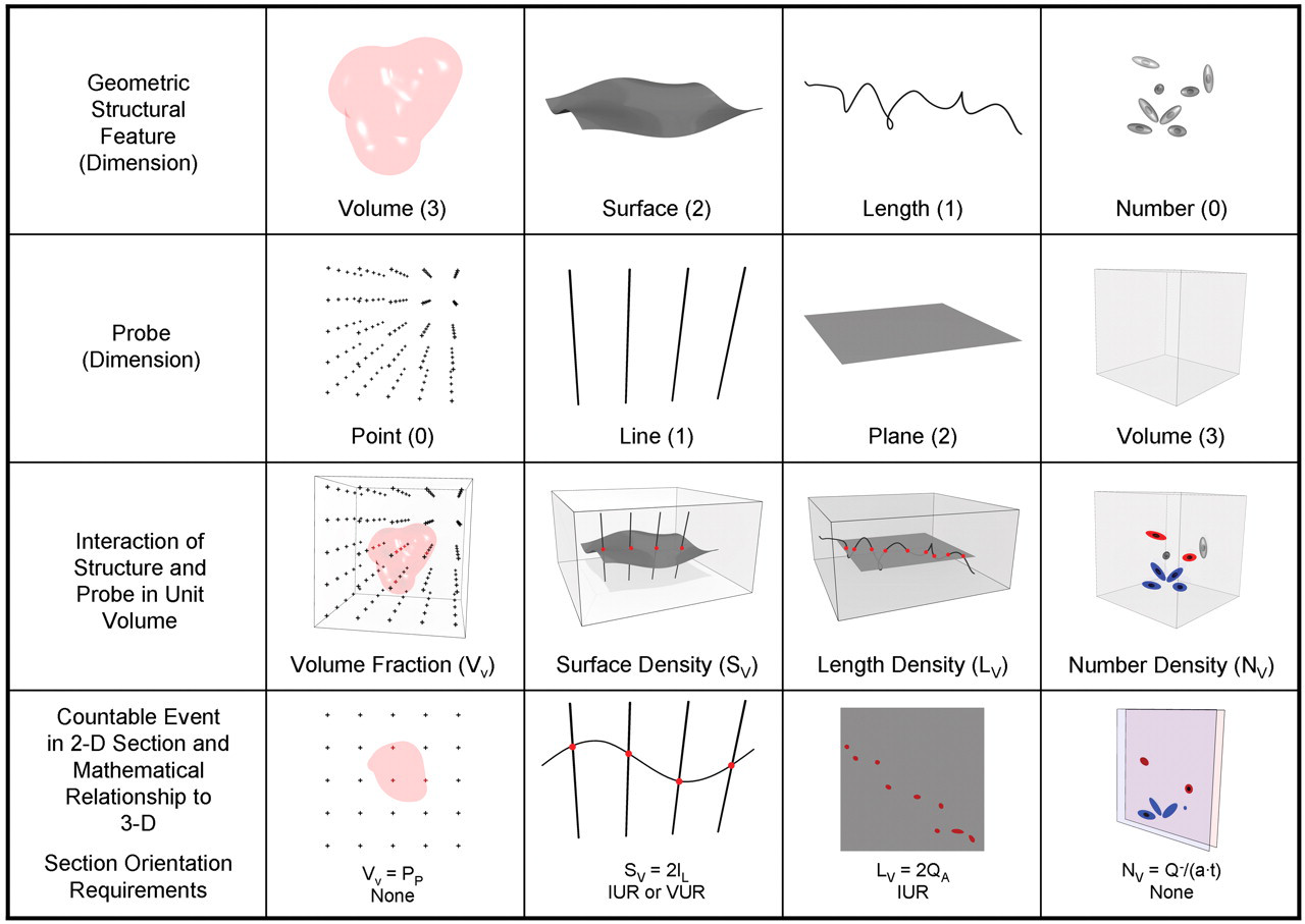
Relationship of geometric structural features and corresponding probes. Top row illustrates the geometric structural features estimated by stereological methods: volume, surface area, length, and number. Second row illustrates the associated probes that sense each geometric feature. Third row is a visualization of probe interaction with the respective geometric feature in 3-D tissue space. Fourth row is the translation of the interaction of probe with geometric feature in 3-D space to the thin histological section illustrating the appearance of each geometric feature in a section, the associated countable events, and the mathematical relationship of the countable events to the quantity of geometric feature in 3-D tissue space. The number of interactions of the probe with associated geometric structural feature is proportional to the quantity of the geometric structure in 3-D tissue space if the sum of dimensions of the geometric structural feature and probe is 3. Quantity of a geometric structural feature is expressed as a density estimate (per unit volume). Volume fraction (V_V ) is estimated from the number of points overlying an object of interest in tissue as a fraction of total number of points overlying reference tissue (P_P ) where V_V = P_P . Surface per unit volume of an object or surface density (S_V ) is estimated from the number of intersections (I) of the object boundary with lines of known length (L) where S_V = 2 I_L . Length per unit volume (L_V ) is estimated from the number of profiles per unit area of section (Q_A ) where L_V = 2 Q_A . Number per unit volume (N_V ) is estimated in a physical disector by counting the number of profiles that are present in one section and not the other consecutive section (Q ⁻ ) with the disector volume defined by the sampled area of the section (a) and section thickness (t) where N_V = Q ⁻ /(a·t). Section requirements are also given for unbiased estimation of each geometric feature. Note that unlike volume and number estimation, section orientation is a significant consideration when estimating surface and length. These geometric features can have preferred orientation in 3-D tissue space. If total length of renal tubules is to be estimated, sections must be produced with random orientation to give all tubules equal sampling probability regardless of preferred orientation in the kidney. These randomly oriented sections used for length and surface area estimation are known as isotropic (IUR) sections (Mattfeldt et al. 1989; Nyengaard and Gundersen 1992) and vertical (VUR) uniform random sections (Baddeley et al. 1986), respectively. Modified from West (1993).

To ensure that probe-structure interactions are random, the position of the relevant probe set is always randomized relative to the structure, that is, the probe sets are randomly positioned onto the sections. For estimation of surface area and length, the 3-D orientation of the probes must also be randomized using simple procedures for rotating the tissue at embedding. All together, these steps form the basis of unbiased “questioning” in design-based stereology.

The unbiased estimation of the last geometric feature, number—a zero-dimensional feature—deserves special consideration. If the dimensions of the geometric feature and its corresponding probe must be 3, a 3-D or volume probe must be used to estimate number. However, it is not possible to probe a single thin histological section with a volume since thin (5-µm) sections are essentially two-dimensional. Therefore, cell number cannot be estimated in a single thin histological section. There is no direct mathematical relationship between the number of cell profiles counted in a single thin histological section and the number of cells that exist in 3-D tissue space. The problem of how to accurately estimate cell number in sections was solved with the development of the disector, a probe based on pairs of thin sections (Sterio 1984). This concept will be further elaborated in discussions on estimation of cell number later in the text.

As illustrated in Figure 6, events are counted in the sections and a mean value is calculated and expressed as a ratio or density, namely, quantity per unit volume. However, to determine whether there is hyperplasia or an increase in total number of cells in the organ, numerical density (number of cells per unit volume) must be converted to an absolute value (total number of cells in the organ) by multiplying numerical density by the reference space (the volume of the whole organ). Failure to convert density estimates to total quantity in the organ can often lead to erroneous conclusions collectively known as the “reference trap” (Brændgaard and Gundersen 1986). Density estimates may be similar between treatment groups, but total cell number can be drastically different because there has been a change in the total organ volume.

Value of Design-based Stereology

The Problem With Counting Cell Profiles and the Solution: The Disector

One justification for investing the time and effort to use stereological approaches may be best supported by considering a frequently encountered issue in toxicologic pathology. Alterations in cell number—hyperplasia, atrophy, or shifts in organ cell populations—can be potentially adverse test article-related effects. Qualitative histopathology has limited sensitivity to detect changes in cell number. Depending on the tissue, the magnitude of the change in cell number must probably reach 25%–40% before it can be appreciated by the pathologist. For example, in a study by de Groot et al. (2005), a 33% reduction in total hippocampal neuron number was not detected even with side-by-side comparison of photomicrographs. If the change in cell number is subtle, sensitive quantitative methods are needed.

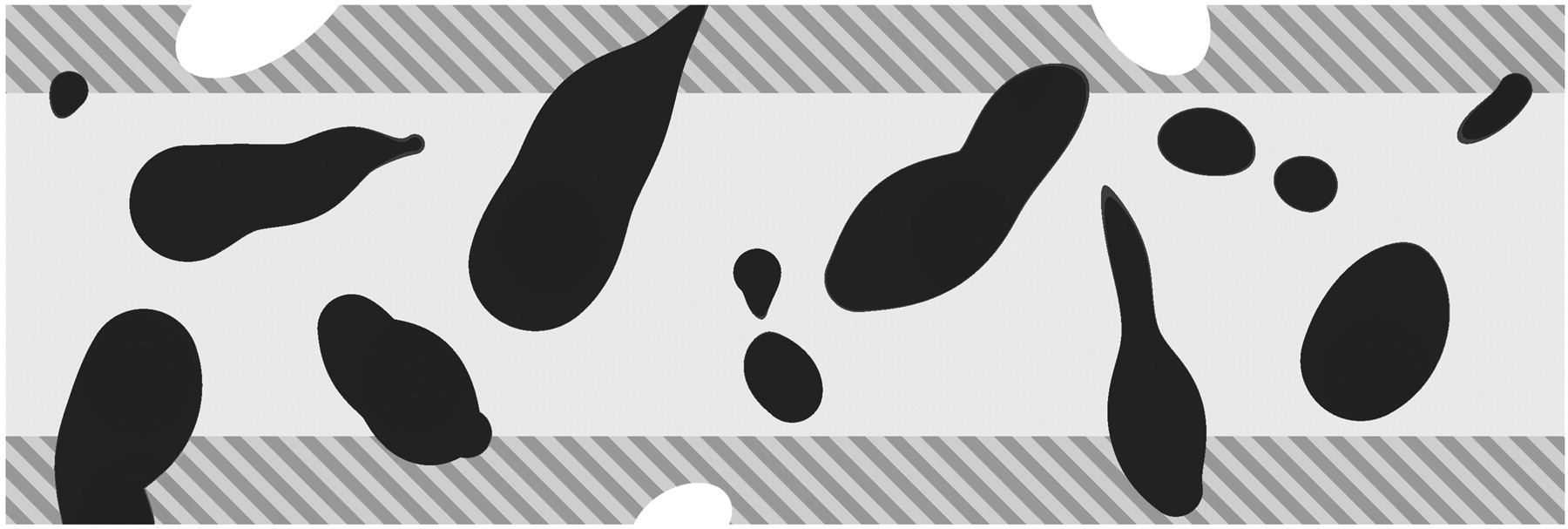
Pathologists have historically relied on 2-D cell profile counts to assess effects on cell number, but because this is a surrogate, assumption-based measurement, it is insensitive to subtle changes. The bias or systematic error associated with 2-D cell profile counts that influences sensitivity is illustrated in Figure 7. When an organ containing three large green cells and four small red cells is serially sectioned, as indicated by the parallel horizontal planes in the figure, a number of profiles are generated in the set of serial sections, as shown. Larger green cells make more profiles and are overrepresented because a section plane samples cells proportional to cell height. Hence, a section plane does not probe or “sense” cells proportional to their number, but rather to their height perpendicular to the section plane. By analogy to opinion polling, the “questioning” is biased toward the larger cells. This bias will not average out by taking more sections and counting more profiles; every section will overrepresent larger cells.

Figure 7.

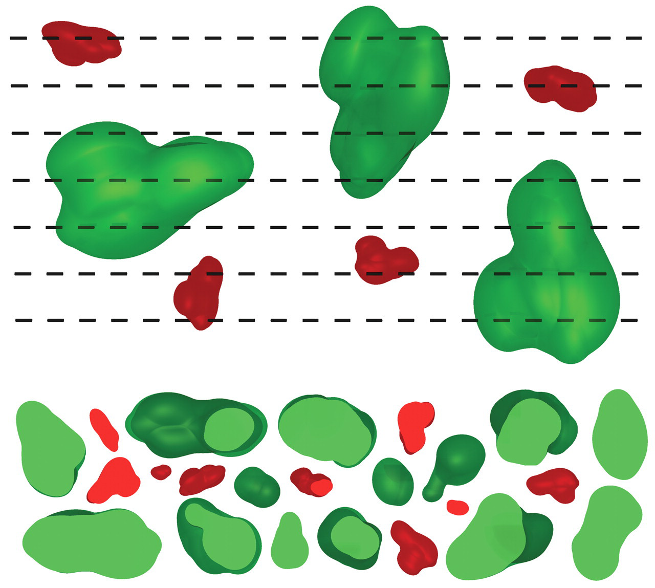
Schematic illustration of how consecutive sectioning cells with 2-D planes samples cells proportional to their height, not their number. A tissue containing a population of three large green cells and four small red cells is sectioned exhaustively by uniform random sectioning planes by the microtome indicated by the parallel hatched lines; the spaces between the lines are thin sections viewed on edge. The total number of profiles of large (fourteen) and small (nine) cells counted on all the sections through the tissue is illustrated (arbitrarily arranged) at the bottom of the figure. All cells are overrepresented and counted more than once, particularly the large green cells. Clearly, the numbers of profiles of the respective cell types do not in any simple way reflect the actual number of these cells or their relative proportion.

As discussed previously, unbiased estimation of cell number requires a 3-D or volume probe. The problem of how to count cells using thin histological sections was solved with the description of the disector (Sterio 1984). Figure 8 illustrates the disector counting principle. The disector consists of (at least) two parallel planes. The physical disector consists of two thin sections separated by a known distance, typically consecutive sections for cell counts. The optical disector consists of a stack of optical sections created by moving a focal plane through a known distance within a thick section. The distance between the tops of the physical sections, or the height of the stack of focal planes, is termed the disector height. The area of the section planes and the tissue between them, the disector height, constitutes a volume of tissue that fulfills the requirement for a 3-D probe. Cells are counted only if they are present in one section, the sampling or counting section, and not in the other, the look-up section. This rule ensures that cells are counted only once and avoids overrepresentation of larger cells. If the organ illustrated in Figure 8 was serial sectioned and cells were counted in consecutive pairs of sections constituting the entire organ using the disector principle, the true number of cells—three green and four red cells—would be obtained.

Figure 8.

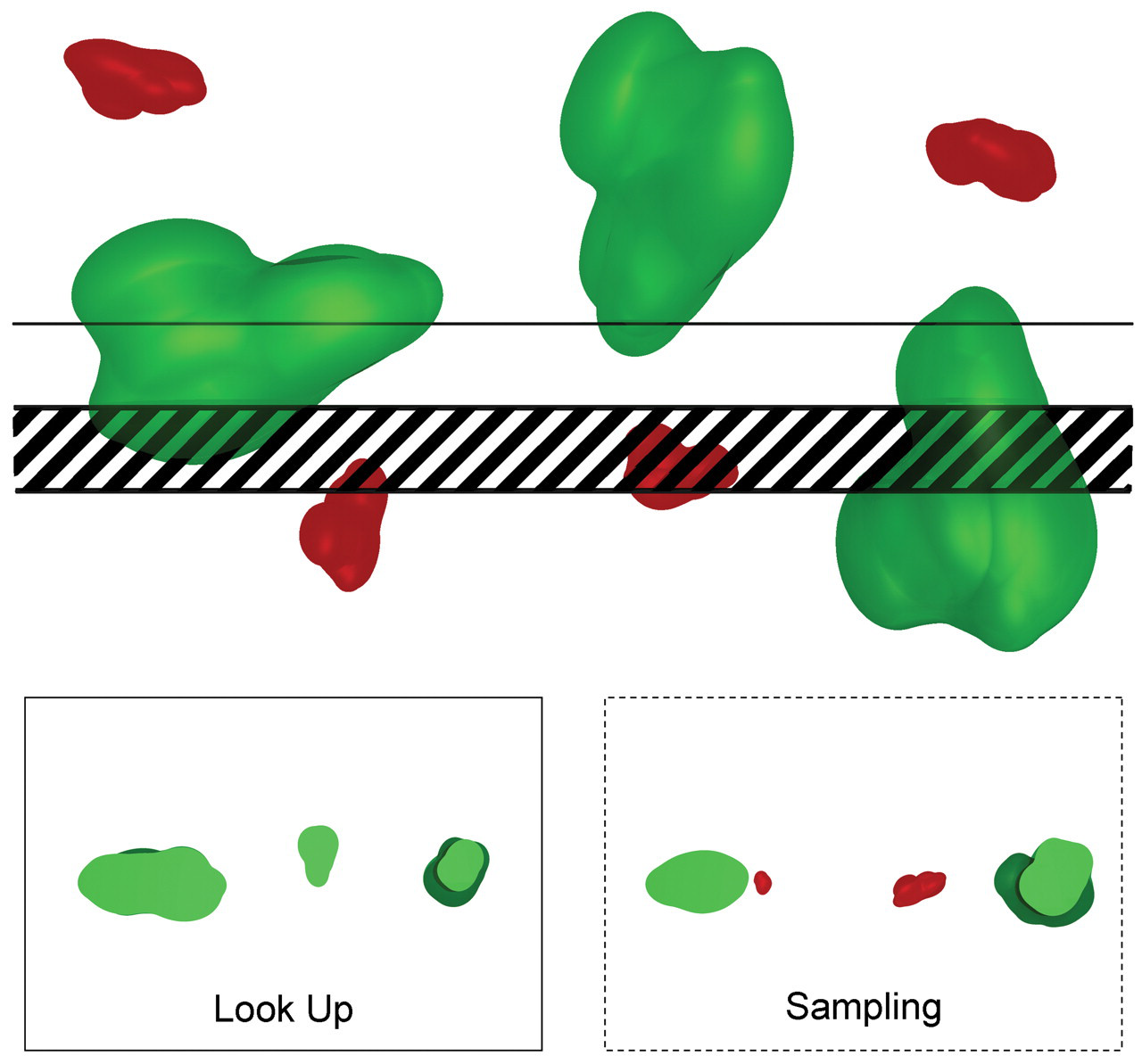
Schematic illustration of the disector principle for sampling of cells proportional to their number. The top figure depicts the tissue consisting of three large green and four small red cells from which two serial sections are collected (seen on edge). The hatched section is the sampling section, and the section immediately above is the look-up section. The profiles of particles present in the respective sections are illustrated in the bottom figures. Particles present in the sampling section are counted only if they are not present in the look-up section. This procedure ensures particles or cells are sampled proportional to their number and not their height perpendicular to the sectioning plane. In this illustration, two (red) particles that are not present in the look-up section are counted in the sampling sections. The area sampled for counting in the section planes and the distance separating them, in this case the thickness of the hatched section, constitute a volume. If the entire tissue was sectioned exhaustively by uniform sectioning planes by the microtome and the disector counting principle was applied to successive pairs of disector sections throughout the tissue, the total number of all cells—here three green and four red—would be counted.

The last component of the disector counting principle is the unbiased counting frame (Gundersen 1977; Figure 9). A counting frame of known area with attendant counting rules ensures only cells that “belong” to the sampled field are counted and thus avoids overcounting. The number of cells is counted that are sampled by the counting frame in the sampling section and not present in the look-up section. This number can be obtained from pairs of consecutive thin sections (physical disector) or while focusing down through a thick section (optical disector). The count divided by the known volume of the disector (calculated as the disector height multiplied by the counting frame area) provides an estimate of the numerical density, N_V . The total number of cells in the organ is then estimated by multiplying N_V by the volume of the organ. Organ volume can be estimated in several ways, as discussed later in the text.

Figure 9.

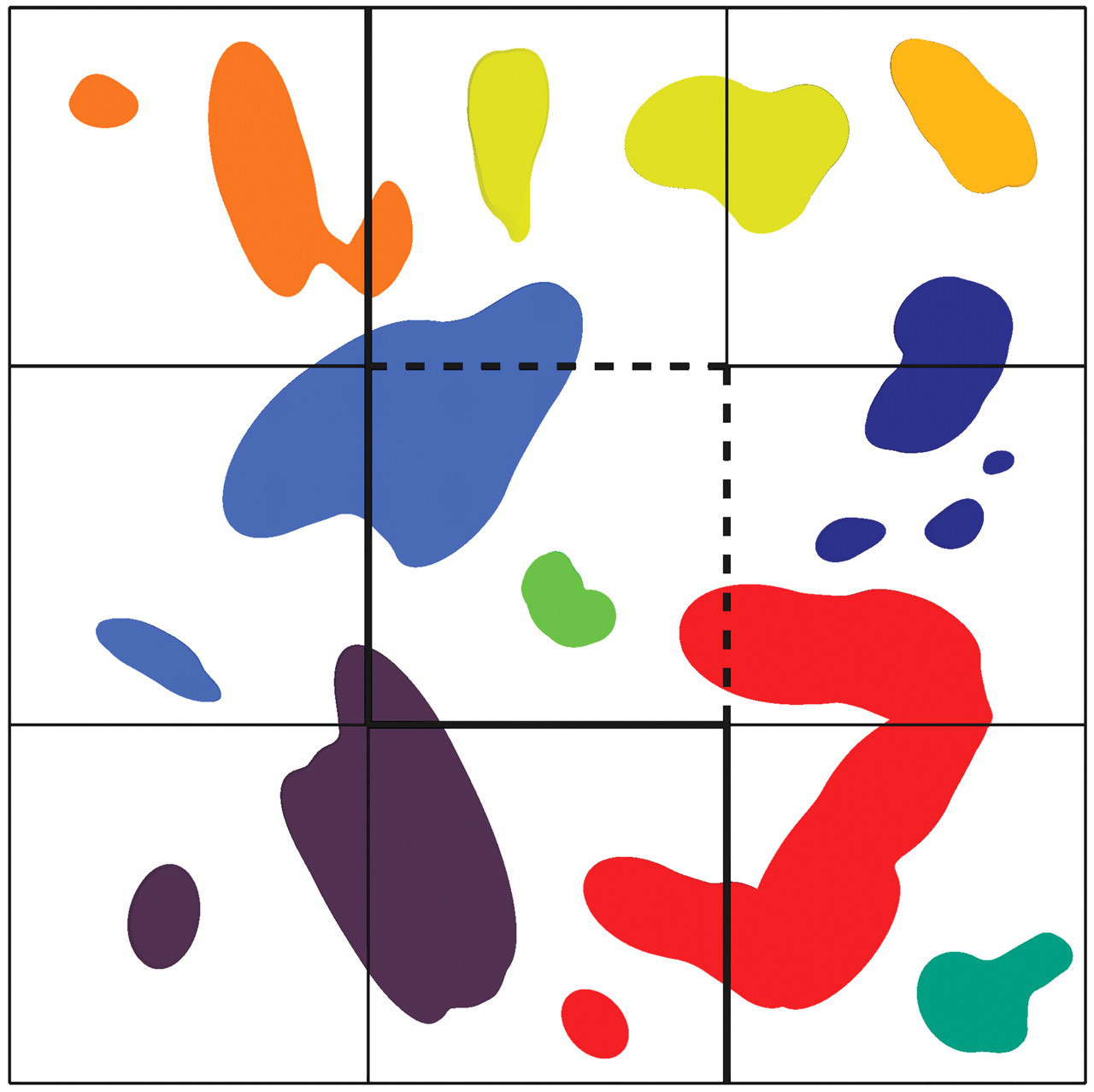
The unbiased counting frame ensures that only objects that belong to the area of section sampled by the frame are counted. The figure shows a tessellation of nine potential sampling sites. The center square is sampled by an unbiased counting frame. Objects that “belong” to each of the nine possible sampling squares have a unique color, indicated by the color of the small object contained entirely in the respective square. The color assigned to the large objects reflects which sampling square they “belong to” using the counting rule of the unbiased counting frame: objects completely or partly contained in the frame (including those touching the dashed inclusion lines) and not touching the exclusion lines or their extensions (thick solid lines) are counted. The illustrated profiles represent the unique counting feature that for cells may be either nucleoli, nuclei, or cell tops.

It is frequently asked how much the bias inherent in the 2-D cell profile counting method affects the estimates and, if comparisons are made to controls, why would the bias not cancel out? Those who use stereological principles rarely compare 2-D with 3-D estimates. However, a few neuroscience studies have estimated neuron number by 2-D and 3-D methods side-by-side. In these studies, estimates of 2-D neuron number were biased by as much as 40% (Coggeshall 1992; Pakkenberg et al. 1991). In a rodent model of testicular atrophy, Mendis-Handagama and Ewing (1990) found 2-D and 3-D estimates of Leydig cell number varied by 100%. These examples illustrate the potential magnitude of the systematic error associated with 2-D methods.

Evaluation of Sampling Variability and Precision of Stereological Estimates

Another justification for using stereological methods is that the sources of variance in a study can be analyzed. Random error resulting from sampling and counting can be assessed for the most commonly used stereological estimators and is expressed as the coefficient of error (CE = SEM/mean). The CE is one of the terms in the essential formula:

${\text{Observed\hspace{0.17em}Variation}}^{\text{2}}{=\text{Biological\hspace{0.17em}Variation}}^{\text{2}}{+\text{Coefficient\hspace{0.17em}of\hspace{0.17em}Error}}^{\text{2}}$

that is, the methodological imprecision is simply added to the biological variation to yield the total variation of the data (when all terms are squared). This simple relation allows the scientist to determine where best to focus efforts to reduce variance and increase precision with optimal efficiency.

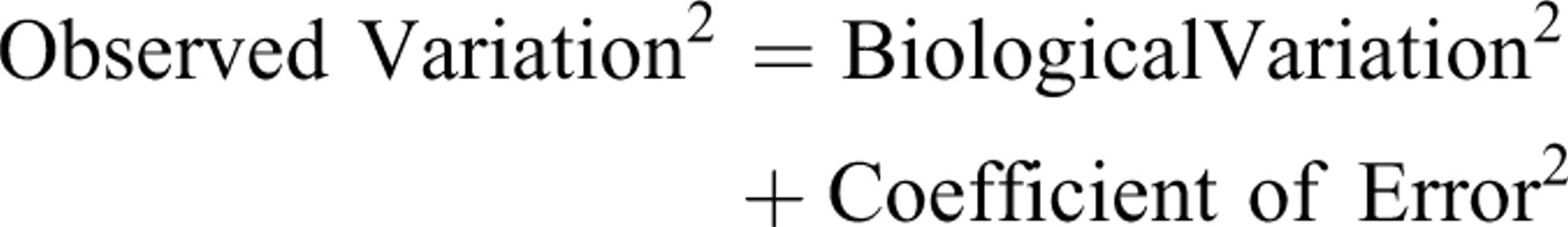
Calculation of CE allows researchers to report stereological data for each treatment group along with the corresponding CE, similar to reporting clinical chemistry data with corresponding confidence intervals. For a simple independent variable, CE is calculated by dividing the coefficient of variation by √n, where n is the number of measurements or counts; CE is reduced proportional to 1/√n. However, the actual formulas to calculate the CE for many stereological estimators are substantially more complex because sampling methods are not independent (recall that with SURS, all sampling positions are random, but fixed relative to each other), and the reader is referred to Gundersen (Gundersen and Jensen 1987; Gundersen et al. 1999) and Cruz-Orive (Cruz-Orive and Geiser 2004) for details. For stereological estimators, CE may be reduced proportional to 1/n ² or even better, rather than just 1/√n underscoring the effects that statistical sampling methods intrinsic to stereological estimators have on precision and efficiency of the analysis methods.

When evaluating sources of variance in a data set, the goal is to optimize sampling and counting to efficiently obtain estimates with acceptable precision. Optimal efficiency is typically achieved when the CE values are ≤ ½ of the observed coefficient of variation. Thus, if the coefficient of variation is ~20%, then a CE of ~10% will typically be of sufficient precision. As previously mentioned, this precision will likely be accomplished with 100 to 200 counts collected from fifty microscopic fields spread across six to ten blocks/sections. To do additional sampling and counting in this situation would be inefficient—wasted time and energy—because the greatest contribution to the observed variation comes from the biological variation that cannot be altered by more sampling or counting. Hence, once a suitable CE has been achieved, the only way to increase the precision of the treatment group mean, that is, to decrease the variance of the group mean (SEM), is to increase experimental group size. This concept is the mantra of design-based stereology—“Do more, less well” (Gundersen and Osterby 1981). It is strongly advisable to obtain information about the biological variation inherent in a given experimental model from a small pilot study. Data about the biological variation in the group and the CE obtained by the stereological analysis from a pilot study will allow the researcher to do statistical planning of the definitive study and to calibrate the sampling methods to generate the most efficient CE. If nothing is known about the biological variation of the structure of interest, it has been suggested that five animals/group and five blocks/animal be used as a starting point (Cruz-Orive and Weibel 1990). By minimizing the contribution of the measurement process to the observed variation and determining the inherent biological variation in a pilot study, definitive studies with suitable power can be designed, thus avoiding waste and unnecessary use of animals in an inadequately powered study. This advice may be most valuable when considering incorporating a stereological endpoint in standard non-rodent toxicology studies in which numbers of animals per group are limited.

Use of Design-based Stereology in Toxicologic Pathology

Tiered Approach for Detecting Subtle Changes

In toxicologic pathology, structural changes in tissue may be evaluated with varying levels of sensitivity. The reference standard is the qualitative/semiquantitative histopathological evaluation by an experienced pathologist. In most cases, this evaluation integrated with other study endpoints has sufficient sensitivity to meet regulatory needs—identify test article–related effects and hazards, define the NOEL/NOAEL, and contribute to weight-of-evidence considerations for risk assessment.

In certain settings, it may be useful to quantify tissue changes appreciated by the pathologist in the optimal routine sections used for histopathology. Such analyses provide detailed information only about those routine 2-D sections and do not convey information about quantities of structures in 3-D tissue space referent to the whole organ. Even with this limitation, further analysis of routine sections can be useful for providing semiquantitative endpoints to support the pathologist’s impressions. For pathologists working with discovery research groups, these types of quantitative endpoints in conjunction with severity grades can assist in conveying the magnitude or extent of changes to non-pathologists. Analyses such as comparative numerical density of Ki-67–positive nuclear profiles on routine sections may have adequate sensitivity to detect a proliferation signal if the test article effect is sufficiently large, for example, three- or four-fold increase. For hyperplasia and atrophy, these data can be further supported by changes in organ weight. However, when data from such analyses indicate small or moderate changes, drawing conclusions from such data can be tenuous. The biases in these cases can influence the results to such a degree that the real change might be directionally opposite. Although 2-D quantitative data can be valuable, the limitations of sensitivity and accuracy should be taken into consideration when using it.

Design-based stereological approaches should be employed when detection of subtle structural tissue changes is critical to the decision-making process. These subtle effects may include adverse, unmonitorable and/or irreversible test article–related changes, and quantitative data may be required to identify a potential hazard or to confirm a NOEL/NOAEL. An example might include identifying a 30% decrease in alveolar number in the developing lung affected by a drug for potential pediatric use, or cases where a quantitative definition of the NOAEL for test article–related hyperplasia and sustained proliferation in an organ is needed to determine appropriate clinical exposures. The magnitude of changes in these cases is below the sensitivity of qualitative pathology and is within the range of the systematic error of biased 2-D methods.

Practical Aspects of Estimation of Cell Number

The Fractionator

The disector principle solved the problem of how to obtain unbiased estimates of cell number in either thick sections or pairs of consecutive thin sections. In the past, total cell number was estimated in a two-step process by first estimating average numerical density (N_V ) and then multiplying by the organ volume. Although a robust approach, this method can be cumbersome because it requires measurement of the total organ volume (reference volume) with careful monitoring of any changes in tissue volume or section deformation that occur as a consequence of histological procedures. Changes in the tissue volume that occur during histological processing can be quite extensive and may significantly affect density estimates. Processing-induced shrinkage is particularly problematic for paraffin embedding, which can cause up to a 40%–50% reduction in tissue volume (Haug et al. 1984; Iwadare et al. 1984; Miller and Meyer 1990). It cannot be assumed that shrinkage effects will cancel out if the tissues from control and test article–treated groups are handled identically. Test articles and disease cause both known and unknown cellular effects that may affect the way a tissue responds to processing and embedding.

Fortunately, a direct estimator, the fractionator, was introduced that obviates issues of tissue shrinkage and section deformation, and the need to estimate total organ or reference volume (Gundersen 1986). The basic principle of the fractionator is that a known fraction of an organ is sampled in one or more sampling steps and in the final sample, the total number of cells is determined using either physical or optical disectors known respectively as the physical or optical fractionator. The total number of cells in the organ is then estimated by multiplying the number of cells counted in the final sample, ∑Q  ⁻, by the inverse of the sampling fraction for each sampling step. As an example, to estimate the total number of cells in an organ, the organ is sampled into slabs, cubes, sections, and microscopic fields with sampling fractions of 1/4 of the slabs, 1/10 of the cubes, 1/200 of the cubes sampled by disector sections collected during exhaustive sectioning, and 1/50 of the section area in which a total of 200 cells (∑Q  ⁻) is counted. The total number of cells in the organ is 4 × 10 × 200 × 50 × 200, for a total of 80 million cells.

The key advantage of the fractionator is that the estimation procedure is insensitive to tissue shrinkage. In the example given above, all tissue-processing shrinkage of the sampled cubes takes place before the disector sections are collected. Because number is zero-dimensional, no matter how the tissue shrinks or deforms during processing or after the sections are collected, the total number of cells present is unaffected and a known fraction is sampled and counted. These features make paraffin sections suitable for use with this estimator, and hence, attractive for use in a regulatory toxicology setting.

Physical Disector and Physical Fractionator

Physical disectors for cell counting typically consist of paired serial 2- or 3-µm–thick sections. These constitute the counting and look-up sections with the section thickness corresponding to the disector height (Figure 10). The optimal height of the disector is generally targeted at 1/4 to 1/3 of the object height. In order of preference, the nucleolus, the nucleus, or cell top can be used as the unique counting feature.

Figure 10.

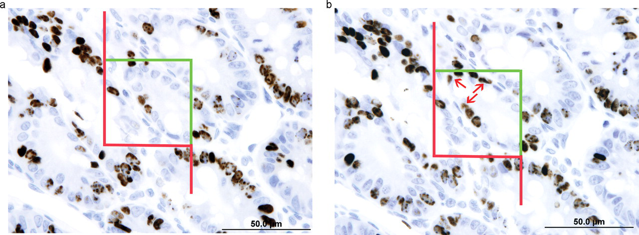
Physical disector consisting of a pair of two consecutive 3-µm sections of BrdU-labeled intestinal epithelial cells. Figure 10a is the look-up section. In Figure 10b, the sampling section, the counting frame samples three BrdU-positive nuclei not present in the look-up section (arrows).

Thin paired serial sections are most easily prepared from plastic or paraffin-embedded tissue. As mentioned, tissue shrinkage with paraffin is a concern if physical disectors are used with the two-step estimation method (Dorph-Petersen et al. 2001) but is not an issue if the fractionator is used. A specific requirement for unbiased cell counts using physical disectors is that section thickness must be constant. Plastic-embedded sections must be cut essentially dry and paraffin sections must be prepared at a constant block temperature (easiest to achieve by cutting at room temperature) to avoid expansion or contraction of the block face, which can cause variation in section thickness. Hydrating the paraffin block face is permissible because it does not influence section thickness.

Physical disectors have several advantages over optical disectors. The use of thin sections mitigates several concerns encountered with thick sections for optical disectors including “lost caps,” z-axis deformation, and adequate stain penetration (see section on optical disectors for details). When paraffin is used, the histological procedures used for physical disectors are in line with routine procedures in a regulatory pathology laboratory, and staining protocols for thin sections are amenable to automation.

On the other hand, when dimensional stability (i.e., no deformation in any dimension) is needed in combination with immunohistochemical stains for estimation of cell size, thick frozen or vibratome sections should be used, and these estimates are ideally obtained from sections using optical disectors (Dorph-Petersen et al. 2001).

In addition to estimation of cell number, the physical disector and fractionator are used to estimate number of bone trabeculae, capillaries, or pulmonary alveoli. The reader is referred to additional references for details of the methods and applications (Gundersen et al. 1993; Hyde et al. 2004; Nyengaard and Marcussen 1993; Ochs et al. 2004).

Simple Physical Fractionator With Exhaustive Sectioning of the Organ

The simple physical fractionator is the most straightforward fractionator design when the entire organ can be processed and embedded in toto, for example, for analysis of small organs or anatomically defined regions of larger organs. The entire organ or region is processed, embedded in paraffin, and subjected to all processing-induced shrinkage before the final samples (sections) are collected during exhaustive sectioning. Paired disector sections are collected at uniform intervals, known as the section sampling period, throughout the organ until the entire region of interest has been sectioned. For example, every 40th section could be collected. Importantly, the first section is sampled randomly within the selected interval, in this case, sections 1 through 40. The section sampling period is typically adjusted to yield a total of eight to twelve disector pairs through the organ. The section sampling fraction is 1 divided by the section sampling period. In the set of disector sections, a known fraction of the area of the sections, the areal sampling fraction, is sampled by an unbiased counting frame and cell number is counted in physical disectors. Total cell number in the organ is then estimated by multiplying the cell number count by the inverse of the section and areal sampling fractions.

As an example, if 2-µm disector pairs are collected every 400 µm or every 200th section, section sampling fraction is 1/200 with a random start. If areal sampling fraction is 2% or 1/50 and a total of 200 cells is counted in those collective sampled areas across the disector sections, then total number of cells is 200 × 50 × 200 = 2,000,000.

Until recently, use of the physical fractionator for estimation of cell number has been limited because registration of high-magnification fields in the paired sections—the counting and look-up section fields—was labor-intensive and time-consuming. However, new software advances now allow for automated sampling, capture, and registration of spatially matched high-magnification microscopic fields, making implementation of the “automated” physical fractionator for cell counts in a toxicologic pathology setting practical and efficient (AutoDisector™, Visiopharm, Hørsholm, Denmark).

Physical Fractionators With Subsampling

To apply the physical fractionator principle to organs or objects of interest too large to embed and section in toto, additional subsampling of tissue prior to embedding is needed. The classic solution to this problem is to perform one or more subsampling steps to reduce the amount of tissue to a set of samples. This set of samples is processed, embedded, and the final sample of the fractionator, the set of disector sections that constitute a known fraction of the embedded tissue samples, is collected during exhaustive sectioning. Although this approach is insensitive to shrinkage, the need for exhaustive sectioning limits efficiency. Fortunately, novel efficient fractionator designs for large organs that avoid the need for exhaustive sectioning have been developed (Gundersen, unpublished). Two fractionator designs using paraffin embedding have recently been implemented (Mirabile et al. in preparation). Methods for generating SURS thick plastic, frozen, or vibratome sections without exhaustive sectioning have been used for years because processing-induced shrinkage is rarely an issue with these embedding formats (Dorph-Petersen 1999; Dorph-Petersen et al. 2007; West and Gundersen 1990).

Physical Fractionator Designs in Toxicologic Pathology

Physical fractionator designs implemented in concert with new software and hardware advances have several potential benefits relevant to toxicologic pathology, including reduced animal usage, accelerated timelines to generate stereological data, and enhanced study documentation. With the simple fractionator design and designs with subsampling, paraffin sections can be simultaneously collected for histopathology from the same animal, obviating the need for satellite groups. Thin paraffin sections reduce time and resources because they are compatible with both automated histochemical or immunohistochemical staining (Lyck et al. 2008). Commercially available software such as the AutoDisector™ software (Visiopharm, Hørshom, Denmark) provides for the automated capture, registration, and archiving of matched high-magnification microscopic fields, where cell counting can be performed offline at leisure. Because thin histological sections are compatible with whole slide imaging technology, rapid sampling can be performed in silico on virtual slide images, thereby increasing throughput and providing for enhanced electronic documentation of stereological procedures in a Good Laboratory Practice environment.

Optical Disector and Optical Fractionator

Optical disectors are created in thick sections by scanning the section with thin optical focal planes using a high numerical aperture oil (or water or glycerol) immersion objective (Gundersen 1986). A 100× oil immersion lens with a numerical aperture of 1.4 has a focal plane of a thickness of ~0.5 µm. As the focal plane is moved a known distance through the section, cells are counted as they come into focus. A unique structural feature of the cell, such as the nucleolus or the large, crisp equatorial profile of the nucleus, is used as the counting feature. Thus, the optical disector is a solution to the original limitation of the physical disector for cell counts, namely, the registration of high-magnification microscopic fields in paired sections.

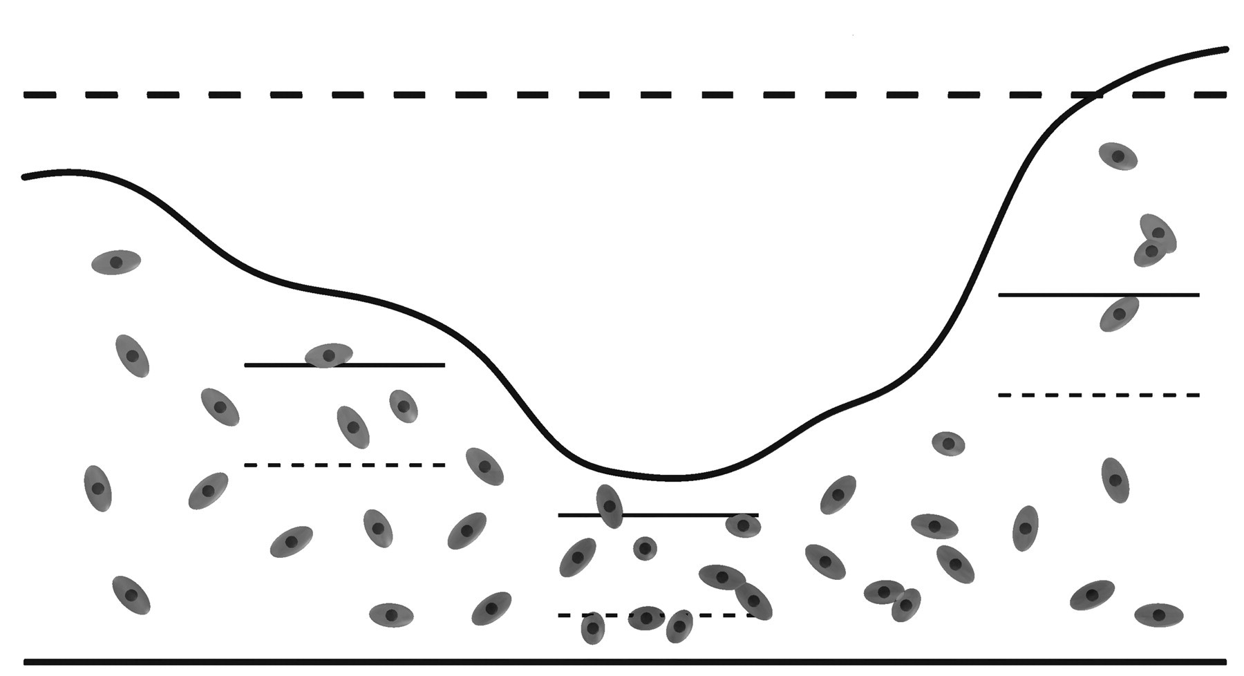
Thick paraffin, plastic, vibratome, or frozen sections may be used for optical disectors. Counts must be confined to the central region of the section as illustrated in Figure 11. The shaded regions at the top and bottom of the section, known as guard zones, are excluded because sectioning can extract parts of whole cells close to the sectioning plane; these extracted cells or parts are known as “lost caps” (Gundersen 1986). The width of the guard zones may vary with tissue and embedding media and can be optimized by performing what is known as a z-axis distribution (calibration) to avoid problems resulting from “lost caps” (Andersen and Gundersen 1999; Dorph-Petersen et al. 2004; see also Figure 4 and corresponding text in Dorph-Petersen et al. 2009).

Figure 11.

Thick section seen edge-on. A defined region of the upper and lower boundaries of a thick section close to the sectioning planes cannot be included in the optical disector. These regions, the guard zones, are excluded because sectioning can remove cells or portion of cells. If guard zones were included, the cell number would be underestimated. The size of the zones depends on the tissue and the preparation. Modified from Figure 2.3 in Gundersen (1986).

Section thickness is a critical consideration. Section thickness at the time of microscopic analysis should typically be a minimum of 25 µm to allow for adequate guard zones and a sufficient disector height (≥ 10 µm). A section thickness of 20 µm may be adequate for plastic sections. With frozen or vibratome sections, shrinkage in the z-axis can be substantial and can potentially be progressive with time following preparation (Lyck et al. 2007), although steps may be taken to reduce z-axis shrinkage and increase section stability (Konopaske et al. 2008 and references therein). If progressive collapse of the section along the z-axis is detected over time, temporal coordination of section preparation and analysis may be required to ensure adequate section thickness at the time of analysis. Depending on the tissue and the staining protocol, frozen and vibratome sections should be cut at 40–80 µm to ensure adequate thickness at the time of analysis. Z-axis shrinkage of frozen and vibratome sections has also been demonstrated to be non-uniform, as illustrated in Figure 12 (Dorph-Petersen et al. 2001). Although local cell counts are influenced by the degree of local deformation, unbiased cell number estimation is straightforward using estimators based on the number-weighted mean section thickness requiring frequent measurements of local section thickness (Dorph-Petersen et al. 2001).

Figure 12.

Thick section sampled by three optical disectors seen edge-on. Non-uniform shrinkage in the thickness of the section (i.e., in the z-axis) can bias cell counts in an optical disector of fixed height. Therefore, the local section thickness must be measured concurrently with cell number to obtain an unbiased estimate of cell number (cf. Eqs. 9 through 11 in Dorph-Petersen et al. 2001). Modified from Figure 1 in Dorph-Petersen et al. (2001).

There are several technical issues to consider when using optical disectors. Because only unambiguously identified objects can be counted, histochemical or immunohistochemical staining protocols used to identify the cell population of interest must be optimized to ensure complete stain penetration through the section. Staining protocols for thick sections sometimes require that sections are stained free floating with extended incubation times and specialized methods are needed for epitope retrieval, mounting, and coverslipping, all of which at present must be done manually (e.g., Lyck et al. 2006; Müller et al. 2001). If vibratome or frozen sections are used, stability for long-term archiving may be a concern.

Optical disectors and thick sections have the advantage of being genuinely 3-D, making it possible to observe cells in their full 3-D extent, allowing for easy and robust cell classification based on morphological criteria. Also, delineation of subtle regions of interest may be easier in thick sections compared with thin sections.

Sampling designs described for the physical fractionator can all be performed with thick sections and optical disectors and is termed the optical fractionator (West et al. 1991). As discussed for the optical disector, a wide range of tissue preparations can be used with the optical fractionator, and it is the preferred estimator if frozen or vibratome sections are required (Dorph-Petersen 1999; Dorph-Petersen et al. 2007; Konopaske et al. 2008). In the past two decades, the optical fractionator has been the gold standard for estimation of cell numbers in experimental biology. It solved the historical limitation of physical disectors for cell counts, namely the co-registration of high-magnification microscopic fields in paired sections. Although the method has gained great popularity in basic research because of its simplicity and efficiency, some of the aforementioned aspects of the optical disectors may limit its utility in a regulatory toxicology setting.

In the optical fractionator, total cell number is estimated as described for the physical fractionator, but because thick sections are used, an additional sampling fraction is included, the height sampling fraction or the fraction of the section thickness used for cell counting in an optical disector. Because non-uniform shrinkage in the z-axis can be observed in almost all thick sections, the height sampling fraction should be calculated as the disector height divided by the number-weighted mean section thickness to mathematically take into account the variations in section thickness and ensure the estimate is unbiased (see Eqs. 9 and 10 in Dorph-Petersen et al. 2001—see also Figure 2 in Dorph-Petersen and Lewis 2010).

Practical Aspects of Estimation of Volume and the Reference Space

As mentioned, total structural quantity in an organ or object can be estimated in a two-step process, (1) by determining mean density (volume, surface, length, or number per unit volume), and (2) multiplying density by the reference volume, that is, the volume of the organ. For isolated organs without cavities and a specific gravity of ~1.0, organ weight can be used to estimate volume. An accurate, precise, and fast assessment of total organ volume is Archimedes' principle of buoyancy determination, which is frequently used for estimation of total lung volume (Dorph-Petersen et al. 2005; Hsia et al. 2010; Scherle 1970).

There is a simple and robust estimator, known as Cavalieri’s Principle, that allows for estimation of volume regardless of how irregularly shaped the object is or if it is contained within a larger structure (Cavalieri 1635; Gundersen and Jensen 1987). The estimation principle involves exhaustively slicing an organ into slabs or sectioning an embedded object with a microtome by a series of parallel section planes separated by a known fixed distance T with the position of the first section plane chosen at random in the interval of 0-T, as described for SURS. The area of the object of interest as it appears on the slab face or histological section is determined, and the sum of the areas multiplied by T is an unbiased estimate of the total volume. Areas can be estimated with an image analysis system or by randomly superimposing a set of points over the slab/section and counting the points overlying the region of interest. Each point has a known associated area (i.e., each point is a square of defined area centered on that point), and total area of the object of interest is estimated by multiplying the total number of points collected across all slabs/sections by the area associated with a point.

When estimating volume from organ slabs, fixed or fresh organs can be stabilized by embedding in 5%–7% low melting point agar to facilitate cutting. One of the cut surfaces of the slabs should be selected consistently for analysis, for example, the posterior cut surface. This convention means that the last organ slice does not contain a posterior cut surface and thus does not contribute to the estimate. A point grid printed on clear acetate film can be placed over the slabs to estimate area (e.g., Jelsing et al. 2005). For small organs or objects contained in larger organs, they can be processed, embedded, and sectioned with a microtome, collecting histological sections at fixed intervals or sampling periods (e.g., every 10th section). The first sample is selected by choosing a random number between 1 and the sampling period (in this case, 1 to 10). The thickness T will be the microtome block advance (which determines section thickness) multiplied by the sampling period (e.g., 5 µm × 10). With histological sections, the point grid is typically superimposed onto a live or captured microscopic image of the section using commercially available software. As noted in Figure 6, there are no special section orientation requirements to estimate volume; therefore, any section orientation can be used. Although the number of counts and sections required to obtain a reasonably precise estimate depends on the complexity of the shape of the structure, a precise estimate can typically be achieved by counting approximately 200 total points collected over six to ten sections (Gundersen and Jensen 1987). Figure 13 illustrates the Cavalieri principle to estimate total volume of a mouse lung.

Figure 13.

Photographic montage showing practical application of Cavalieri’s principle to determine total volume of a mouse lung. A complete mouse lung was fixed by infusion under pressure and embedded in agar, and slabs of constant thickness (T) were prepared with a random start. A set of points printed on a sheet of clear acetate was superimposed over the slabs, and the number of points overlying lung parenchyma is counted, in this case, 172 points. Total volume is estimated by summing the number of points across all slabs (172), multiplying by the area associated with each point, then multiplying by T.

When estimating volume or a structural density in processed tissue sections, it is important to avoid or monitor shrinkage or swelling of the tissue during processing and section preparation. Shrinkage is minimized if plastic, frozen, or vibratome sections are used and carefully processed (Dorph-Petersen et al. 2001). Archimedes' principle can be used to track processing-induced shrinkage (Dorph-Petersen et al. 2005).

Conclusions

Design-based stereology provides a powerful set of tools for quantitative analysis of 3-D tissue structural changes from histological sections that should be part of a tiered morphological approach in regulatory and investigative toxicologic pathology. When properly implemented, these sensitive and efficient methods provide precise estimates with the guarantee of accuracy. Stereological approaches for estimation of cell number, once cumbersome and time-consuming, are becoming efficient and practical to implement in a regulatory toxicology setting. It is now feasible to generate estimates of cell number in a time-effective way using thin paraffin sections by integrating precise and efficient stereological methods with automated whole-slide imaging, automated section sampling, computer-assisted measurements, and automated capture and registration of physical disectors. These advances, however, do not eliminate the first requirement for obtaining accurate estimates—the whole organ must be available for sampling. Prospective planning has been simplified with the development of new sampling methods that can facilitate collection of samples at necropsy for potential future analysis.

Selected Review Articles and Textbooks on Stereology

Cruz-Orive, L. M., and Weibel, E. R. (1990). Recent stereological methods for cell biology: a brief survey. Am J Physiol 258, L148–56.

Gundersen, H. J. G, Bendtsen, T. F., Korbo, L., Marcussen, N., Møller, A., Nielsen, K., Nyengaard, J. R., Pakkenberg, B., Sørensen, F. B., Vesterby, A., and West, M. J. (1988). Some new, simple and efficient stereological methods and their use in pathological research and diagnosis. APMIS 96, 379–94.

Gundersen, H. J. G, Bagger, P., Bendtsen, T. F., Evans, S. M., Korbo, L., Marcussen, N., Møller, A., Nielsen, K., Nyengaard, J. R., Pakkenberg, B., Sørensen, F. B., Vesterby, A., and West, M. J. (1988). The new stereological tools: Disector, fractionator, nucleator and point sampled intercepts and their use in pathological research and diagnosis. APMIS 96, 857–81.

Howard, C. V., and Reed, M. G. (2005). Unbiased Stereology, Three-dimensional Measurements in Microscopy. 2nd ed. Garland Science/Bios Scientific Publishers, Abingdon, UK.

Mühlfeld, C., Nyengaard, J. R., and Mayhew, T. M. (2010). A review of state-of-the-art stereology for better quantitative 3D morphology in cardiac research. Cardiovasc Pathol 19, 65–82.

Nyengaard, J. R. (1999). Stereologic methods and their application in kidney research. J Am Soc Nephrol 10, 1100–23.

Weibel, E. R., Hsia, C. C. W., and Ochs, M. (2007). How much is there really? Why stereology is essential in lung morphometry. J Appl Physiol 102, 459–67.