Sage Journals: Discover world-class research

Abstract

Previous research shows that men’s and women’s employment situations can affect the stability of marital unions, but results differ by country context and different measurements. This study models the effect of spouses’ employment situations on the risk of divorce. It focuses on time aspects and financial aspects, resulting from the employment situation of married spouses in Germany. A broad variety of employment indicators measured in a dyadic perspective lead to an array of hypotheses about marital stability. Event history models on the German Socio-Economic Panel (SOEP) data show mixed evidence for spouses’ permanency of the job and their relative income. Marriages of couples with higher income are more stable. In addition, the spouses’ employment situation does not seem to affect marital stability. The study shows that the precarious job characteristics, which can destabilize marriages in analysis at the individual level, become blurred in analyzing dyads in a 1.5-earner society.

Keywords

divorce/separation financial stress work stress dyadic couples’ employment situation

Introduction

As a consequence of labor market reforms in 2002–2005, fixed-term and temporal employment as well as part-time employment are increasing in Germany (Dietz et al., 2013). Empirical studies have shown that precarious employment conditions are related to financial worries (Mau et al., 2012) and detected an association between the employment protection legislation and well-being (Karabchuk, 2016). Thus, in Germany, the average job stability is high, individuals perceive their jobs to be insecure (Erlinghagen, 2007). Studies have shown that this perceived job insecurity is higher among employees holding fixed-term contracts compared to them holding permanent contracts (Balz, 2017; Erlinghagen, 2007).

Germany has had a very long tradition of following the pathway of a strong male-breadwinner model (Ostner & Lewis, 1995), which implies “breadwinning for men and caring/homemaking for women” (Lewis, 1992, p. 161). However, over recent decades, there are increasingly more women in employment (Brenke, 2015), and Germany has a high proportion of part-time employed persons, even higher than the European average (OECD, 2014). Presently, Germany can be described as a “modified male-breadwinner” country that is characterized by full-time employed men and part-time employed women (Trappe et al., 2015).

Additionally, the family landscape has become more diverse in the past decades, as divorce rates across Europe have been increasing for decades and continue to rise in most countries (cf. Euro 18 countries, Eurostat, 2016) but seem to level off in Germany and few other northern European countries in the 2000s (BiB, 2018; Eurostat, 2016). Studies have shown an increase in divorce risk resulting from women’s employment (Ruggles, 1997; South, 2001), but, as a literature review has shown, findings are inconclusive. This finding has led to the conclusion that the marital dependence hypothesis, which was applied mainly in previous research, cannot explain the association of (women’s) employment and divorce risk (Özcan & Breen, 2012). Furthermore, most couples are not only affected by one spouses’ employment situation and the decision to divorce is made by both spouses, or at least the actions of both spouses can lead to divorce. The dual-earner situation can put a strain on couples because they have to organize the division of domestic tasks and eventually childcare. However, the chance that at least one spouse perceives his/her job as insecure is high in the “modified male-breadwinner” country. Therefore, it seems to be important to analyze the information on couples’ joint situation on their marital stability.

Until today, few studies take both spouses’ labor market situations into account (Blossfeld et al., 2001; Cooke, 2004; Cooke & Gash, 2010; Poortman, 2005a; South, 2001). Those that do, analyze aspects of the couple’s employment situation (Cooke, 2004; Jalovaara, 2003; Raeymaeckers et al., 2006; South, 2001), focus on spouse’s transitions between full-time and part-time work (Blossfeld et al., 2001), or focus on marriages in their first years (Poortman, 2005a). To my knowledge, there is only one study on Belgian couples that models spousal dependency (Raeymaeckers et al., 2006) and one study on spouses divorced between 1991 and 1993 in the dual-earner society of Finland respecting their socioeconomic position (Jalovaara, 2003).

The aim of this study is to apply a dyadic perspective on couple’s risk of divorce by investigating the interplay of both partner’s employment situations and possible effects on the risk of divorce in Germany. I extend existing research by analyzing various dimensions of employment from combined perspectives of husbands and wives and acknowledge the dependency between spouses by testing whether specific combinations of couples’ employment situation that can strain in time and financial aspects may destabilize marriages. In applying stress theories to an association that was investigated mainly in the light of spouses’ economic dependence, I can add to previous discussions. Finally, I answer the question if precarious job characteristics straining spouses in terms of time and financial insecurity are associated to marital instability.

In outlining the results of previous research on this topic, especially from international studies concerning the dyadic perspective, and some German research focusing mainly on the wife’s employment situation and divorce risk, I highlight important indicators to measure a couple’s employment situation. The theoretical framework I develop encompasses stress theories. From these theories, I derive hypotheses, which refer to dimensions of workload, employment instability, and income. Using data from the Socio-Economic Panel (SOEP) on working-age married couples, I employ event history models to test the hypotheses. Finally, I discuss the findings in light of previous research and theory, the case of Germany and in general.

Background

Stress theories play an important role in explaining marital stability in arguing that marital quality is a key dimension of marital stability. Stress theories postulate spill-over effects from external stress into the couple, which lowers marital stability (Aneshensel, 1992; Randall & Bodenmann, 2009). But what is stress, how does it emerge, and how does it affect relationships? Stress can be defined as an internal arousal or process; it emerges from external conditions that differ from individuals. External conditions leading to stress are so-called stressors (Aneshensel, 1992; Story & Bradbury, 2004). A potential stressor is the employment situation, economic hardship, or financial strain (Conger et al., 2010; Randall & Bodenmann, 2017). However, an individuals’ response to stressful events or external conditions is distress. In other words, stress is the internal process that occurs due to stressors and leads to distress. Distress emerges in individuals who are not able to cope with the stress. That means: each individual reacts different on stressors. Distress is a subjective reaction on objective stressors. A strand of theoretical frameworks (e.g., the Vulnerability–Stress–Adaption model by Karney and Bradbury (1995), the Family Stress model (Conger et al., 2010), and the Stress–Divorce model by Bodenmann (1997, 2009) take into account couples as a dyad who have to cope with stress. While the Stress–Divorce model distinguishes stressors along the dimension of exposure to the stressor (chronic or acute), the locus of stressors (inside or outside the couple), and its intensity (major or minor) (Randall & Bodenmann, 2017), the Vulnerability–Stress–Adaption model does not take into account the exposure of a couple to stress (Karney & Bradbury, 1995). However, the Stress–Divorce model postulates that especially long-lasting everyday hassles are damaging relationships (e.g., external chronic minor stressors), as couples’ communication or well-being worsens, or their time spent together is reduced. This leads to mutual alienation and lowers spouses’ marital satisfaction. If couples are not able to cope with the stress, it increases the risk of divorce according to the Stress–Divorce model. As the employment situation is an acute and minor stressor in the understanding of this theoretical framework, spouses’ employment can increase the risk of divorce.

Vulnerability and coping is also important in the Vulnerability–Stress–Adaption model. It is distinct from the Stress–Divorce model as major stressors are the dominant source of stress. The model assumes that stressful events are linked to marital interaction and coping behavior. Marital interaction and coping is part of the adaptive process in a couple and directly linked to martial quality, which is the key determinant of marital stability (Karney & Bradbury, 1995). Both Vulnerability–Stress–Adaption model and the Stress–Divorce model argue that external stress, which can emerge due to the employment situation, spills over into couples, leading to lower marital quality.

Marital quality and stability is affected by stress in the Family Stress model (Conger et al., 2010). Dissimilar to the Vulnerability–Stress–Adaption model and the Stress–Divorce model, the Family Stress model argues that stress affects marital stability and quality indirectly via a worsened marital communication, and spouses’ behavior emerges from financial aspects (Conger et al., 2010). In this framework, couples that are successful in coping are framed as resilient couples to stress. The resilience highly depends on resources (Conger & Conger, 2002). Comparable to the models described earlier, the Family Stress model argues that stressors producing distress in individuals affect the couple as a dyad via their behavior and communication. In the understanding of this framework, economic hardship is an objective measure as families fail to make ends meet or are not able to pay their bills. Exposure time to stress is not directly addressed in the theoretical model. However, as low income and negative economic events are potential stressors, one can conclude that chronic and acute stressors are important resources straining couples.

Stress from workday affects relationship behavior negatively (Buck & Neff, 2012; Schulz et al., 2004), leading to marital conflicts and reducing marital quality and stability (Conger et al., 2010). In dual-earner couples, work stress accumulates from both spouses as they are both exposed to it. Additionally, the time spent together is reduced if both spouses are employed (Poortman, 2005a) because the domestic tasks have to be done after work. This reduced joint leisure time can lead to mutual alienation and consequently to divorce (Randall & Bodenmann, 2009). As coping plays a central role, stress only leads to mutual alienation if the couple is not able to cope with this stress. However, if the couple has enough time and resources for coping, stress does not compulsorily lead to negative consequences. However, in dual-earner couples, negative relationship behavior due to daily work stress should be more prone as in traditional earner couples.

Coping resources are discussed to be varying across social strata. In other words, some research has shown that socially disadvantaged individuals are more prone to suffer from stressors as their coping resources are lower compared to socially advantaged groups (Conger et al., 2010). Similarly, the Vulnerability–Stress–Adaption model assumes individual’s stable characteristics making them vulnerable to stressful events and unable to cope with these events in a relationship (Karney & Bradbury, 1995). Economic hardship is identified as a chronic stressor (Aneshensel, 1992), increasing the couples’ (perceived) economic pressure. The Family Stress model assumes that economic pressure leads to marital problems and ends in lower marital quality and stability (Conger et al., 2010). Poor working conditions produce economic hardship through low income or through work instability (Conger et al., 2010); thus, an uncertain employment situation leads to stress (Aneshensel, 1992). If both spouses are employed, a couple’s potential strain from the working environment and therefore sources of stress are higher compared to traditional couples.

Comparable to Poortman (2005a), in the following, I distinguish stress produced by (a) a reduction of time spent together and an accumulation of daily hassles from work life in terms of workload (time stress) and (b) financial pressure due to insecure and low income (financial stress).

Workload and Divorce

Women’s employment situation is an indicator of reduced time a couple can spend together and can produce an accumulation of work stress in couples where both spouses are employed. In the United States, there is evidence of a significant positive effect of women’s employment on divorce risk (South, 2001). However, women’s employment only affects marriage stability negatively if spouses are unhappy in their relationship in the United States (Schoen et al., 2002). From the Netherlands, it is known that the higher divorce risk of full-time employed women is partly a behavior undertaken in anticipation of divorce. But even for employed women who do not expect a divorce, marital stability is lower (Poortman, 2005b). Studying dyads show a stabilizing effect on marriages when both spouses are employed (Jalovaara, 2003; Raeymaeckers et al., 2006). Cooke et al. (2013) point out that there is no significant effect of women’s employment on divorce risk in Germany. Other findings show a positive effect on divorce risk for full-time employed women compared to part-time employed women in Germany (Böttcher, 2006; Cooke & Gash, 2010; van Damme & Kalmijn, 2014). As part-time work is the most common employment situation of women with children in West Germany (Kreyenfeld & Geisler, 2006), it seems to be a strategy to reconcile family and work (Cousins & Tang, 2004). Therefore, it is important to consider parenthood status in analyzing the interrelation between employment situation and marital stability. Studies have shown that children stabilize marriages (Lyngstad & Jalovaara, 2010; Wagner et al., 2015; Wagner & Weiß, 2003), especially if the children are preschool aged (Steele et al., 2005). However, caring for children also takes time and should increase time stress.

Workload, considered as the number of working hours, seems to have negative effects on marital stability (Böhm et al., 2010; Teachman, 2010). This is true for women (Poortman, 2005a) and mothers (Cooke, 2004), while a higher number of working hours for men reduces divorce risk (Poortman, 2005a).

The evidence of a stabilizing effect of women’s part-time work and mothers with lower working hours can be interpreted in terms of time stress that arises in couples due to labor and domestic tasks. In dual-earner couples, common leisure time is lower than in breadwinner families. More working hours, children, and working overtime can increase time stress of couples. From the time stress argument, I derive two hypotheses: the higher the workload of couples, the higher their divorce risk (H1). This association should be stronger in couples with children because the level of time stress is assumed to be higher in marriages with children (H2) (see Figure 1).

Figure 1.

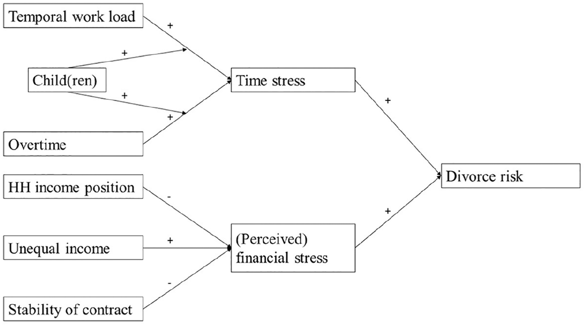
Underlying theoretical concept: How spouses’ employment situation produces stress and its association to divorce.

Employment Stability, Income, and Divorce

As mentioned earlier, stress theories assume that an uncertain employment situation produces stress in couples. Temporarily employed persons are uncertain about their future income and suffer from financial worries about the time after their current working contract (Mau et al., 2012). Perceived financial stress can occur (Aneshensel, 1992; Randall & Bodenmann, 2009): employees with unstable employment situations are under pressure to perform well in the job and, therefore, their work-related stress may spill over to their relationships. Also, Oppenheimer’s (1997) amplified framework of the microeconomic theory argues for a financial stress mechanism that emerges due to unstable employment. An unstable employment situation can endanger a family’s wealth, if the contract is not be renewed or the employed spouse whose employment is unstable cannot find a new job, and the family loses its income. These cases reduce the gain from marriage, and divorce becomes more probable due to greater post-marital alternatives and the expected gains from these alternatives (Becker et al., 1977). However, in collaborating partnerships, dropping out of the job of one spouse and the associated income loss seem less problematic when compared to a drop out in specialized marriages that base their wealth on one job (Oppenheimer, 1997). Congruently, recent research shows a negative effect of employment instability in terms of unemployment (Franzese & Rapp, 2013) as well as feelings of job insecurity (Wagner & Weiß, 2010) on marital stability. Other precarious employment characteristics like fixed-term contracts compared to permanent contracts (Böhm et al., 2010) and an unstable income over the past 12 months (Kaplan & Herbst, 2015) also show negative effects on marital stability. Moreover, temporary workers report negative effects of their atypical working situations on their relationships in problem-centered interviews (Niehaus, 2012).

Couples who depend on one income suffer more from financial stress compared to couples with equal income (Oppenheimer, 1997). Previous research concerning the provision of income in couples shows on the one hand that unequal income can strain couples if the wife provides more income (e.g., Cooke, 2006; Jalovaara, 2003; Kalmijn et al., 2007; Teachman, 2010), but also that higher male income stabilizes marriages (Böhm et al., 2010; Jalovaara, 2003; Kaplan & Herbst, 2015). On the other hand, findings on equal income provision are mixed. While some studies show a negative or no effect of equal income on marital stability (Raeymaeckers et al., 2006; Schoen et al., 2002), others show a higher divorce risk for these couples (Kaplan & Herbst, 2015; Rogers, 2004).

However, economic hardship produces stress in couples. In couples with low household income, financial stress is higher as the couple may worry to make ends meet (Conger et al., 2010). Congruent to the assumptions of the Family Stress model, empirical evidence has shown a decrease in divorce risk with greater household financial resources (Kalmijn et al., 2007; Kaplan & Herbst, 2015; Poortman, 2005a).

In conclusion, marriages with unstable employment of at least one spouse, low household income, as well as a dependence on one spouses’ income can suffer from financial stress. The financial stress can strain couples and put their marriage at risk of dissolution.

Following the financial stress mechanism, I assume that decreasing stability in a couple’s employment situation increases the risk of divorce (H3). Unstable employment situations of spouses can increase perceived financial stress because people in fixed-term contracts have only stable income for the time of the contract. The spouses need to provide savings in case of unemployment after the contract ends. The couples cannot plan with their full amount of income for future investments. Financial stress can also occur in couples with unequal income structure. I postulate a higher risk of divorce for couples with traditional income structures or with higher female incomes compared to those with equal income structures (H4). Furthermore, I expect that the higher the couple’s socioeconomic position, the lower the divorce risk (H5) because couples with a higher socioeconomic position should have less financial stress in comparison to marriages in lower socioeconomic positions.

To sum up, in this study, I assume that chronic external stress produced by the spouses’ employment situation spills over into the couple and lowers marital stability. However, while my theoretical model refers to stress, a subjective feeling, or arousal, the indicators I employ to test the hypotheses measure potential stress sources objectively.

Materials and Methods

Data

The empirical analyses are conducted on data from the SOEP (v32)—a survey conducted since 1984 in West Germany and since 1990 in East Germany (Schupp et al., 2017; Wagner et al., 2008). This panel includes employment history and biographical family background of the respondents. As a household panel, these data are available on a dyadic level as long as a couple shares one household. In this study, I consider couple dyads that are in their first marriage (both spouses) and only those couples married since 1985 or later in West Germany, and since 1990 or later in East Germany. Couples married in 1984 are not considered in the analysis because the information on the permanency of the working contract is conducted since 1985. Furthermore, I focus on couples where none of the spouses has retired. Therefore, the sample consists of 4,932 couples (24,739 couple-years).

Outcome Variable

In this article, the event “divorce” is defined as a legal divorce or a separation of married spouses. The date of divorce defines the end of a relationship if the separation date is not available in the data.¹ In total, 354 (6.8%) out of these 4,932 married couples end in a separation or divorce in the observation window. The mean duration of the marriages observed during the study interval is approximately 11 years (x̅ = 10.85).

Predictor Variables

Predictor variables are operationalized for the couple as a unit (for an overview, see Table A1). All of these predictors are time dependent. Thus, the main predictors of my analysis are five indicators that depend on the characteristics of both spouses.

To measure the dimension of working hours, I use the couple’s temporal workload, on the one hand. This variable is operationalized categorically and (mostly) gender sensitive as either both spouses full-time (1), one spouse full-time and the other part-time employed (1.5 earner) (2), the male spouse full-time and the female spouse not employed (male breadwinner) (3), the male spouse not employed and the female spouse full-time employed (female breadwinner) (4), or both spouses working part-time or less (5). The group of not employed includes unemployed and not employed people, as well as people on maternal leave, in vocational training, or marginally or irregularly part-time employed.² On the other hand, I measure workload with a variable that indicates if the spouses are working overtime. For this analysis, working overtime is defined as working at least five hours per week or more than the fixed time in the working contract. The self-reported information of the respondent concerning overtime work is used.³ If at least one of the spouses works overtime in year t, the indicator is 1, and otherwise zero.

Type of contract indicates the dimension employment stability with regard to holding a fixed-term, permanent, or no contract. Holding no contract also includes people who are self-employed, on maternity leave, or in vocational training. Combining the male and female spouses’ contract types results in three categories: both holding permanent contracts (1), one spouse holding a permanent and the other no contract or a fixed-term contract (2), and couples in which both spouses do not hold a permanent contract (3).⁴

I use two indicators to measure income: The first is gross income relative to spouse. This indicator has three categories. If the husband earns more than 60% compared to the income of his wife, the marriage is considered traditional and categorized in the “husband more” group (1). Couples with equal income where the husband earns 40–60% compared to his wife’s gross income suggests the marriage is in the “about equal” income group (2). Nontraditional couples where the wife’s income is more than 60% of her husband’s gross income are placed in the “husband less” income category (3). The second income indicator is the household’s income position. The household income position is operationalized as a categorical variable and indicates the income quartile (0%–25% (1), 26%–50% (2), 51%–75% (3), and 76%–100% (4)) the marriage unit has in year t compared to the other marriages in year t. The household income position is based on the sum of income from all household members after taxes and government transfers (Grabka, 2016).

Children can also affect the time stress in marriages. Especially, younger children increase the time stress of parents because of the higher caring obligations of younger children. Thus, I include the presence of preschool children, which are children aged under 7 years. I generate a dummy variable that changes in the year of childbirth from 0 to 1. I use childbirth-date data and only include valid cases (don’t know and implausible values were deleted). This variable does not distinguish the number of children. I measure homeownership based on dwelling type. I use the information from the “generated household data set” (hgen) and have a dichotomous variable, indicating whether the couple are joint-resident homeowners or renters, including main tenant, subtenant, tenant, or resident of a home or institutional living facility. In the analysis, the variable region indicates if the household is located in Western or Eastern Germany.

Method

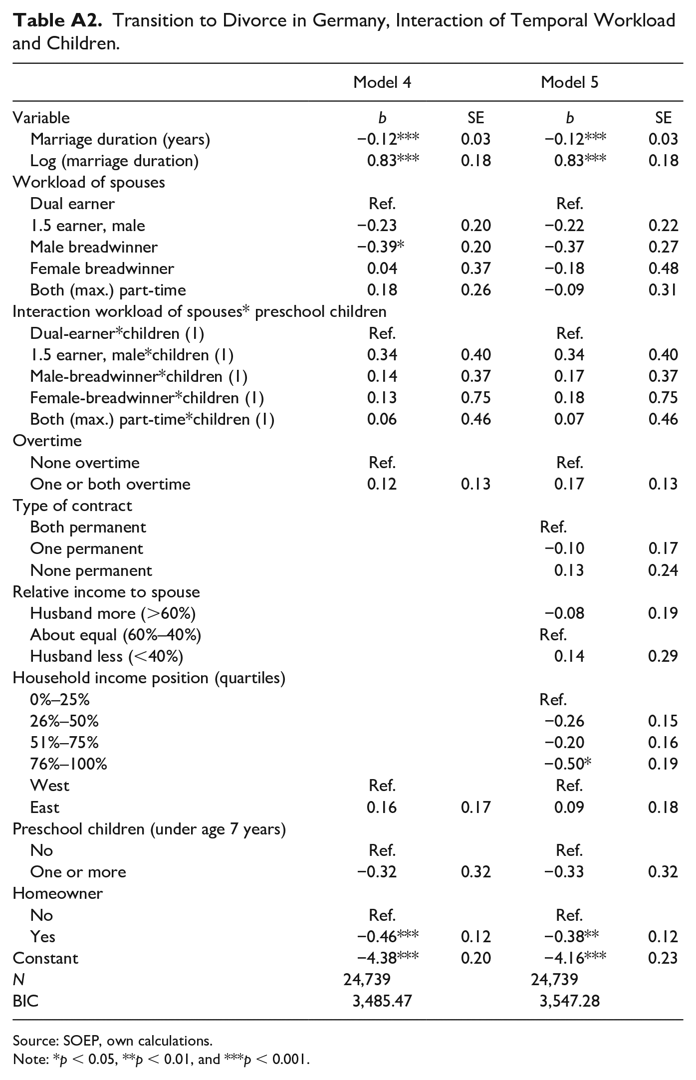
In the first step, I describe couples’ job characteristics based on the couple–year data of first marriages. In the second step, I run stepwise binomial discrete-time event history models on the couple–year data (Allison, 1982, 2014; Singer & Willett, 2003). These models estimate the conditional probability that a couple divorces at time t, given that this couple has not already divorced. Due to the sickle-distributed divorce risk of couples (Kulu, 2014), I include marriage duration and its logarithm into the multiple estimations. Altogether, five event history models are estimated. I report the odds ratios of the models from 1 to 3 (Table 2) and b-coefficients of the models 4 and 5 (Table A2) that estimate the interaction of workload and children. I employ the discrete-time event history models on the time stress indicators (model 1) or financial stress indicators (model 2), including marriage duration, its logarithm, and the control variables of preschool children, region, and homeownership. Model 3 indicates the full model, including all predictors of time stress and financial stress, the marriage duration, its logarithm, and controlling for presence of preschool children, homeownership, and the region. Model 4 is again a reduced model that estimates an interaction between the workload and the presence of children under 7 years, and model 5 is the full model including, besides all other predictors of spouses’ job characteristics, the interaction term of workload and children.

Results

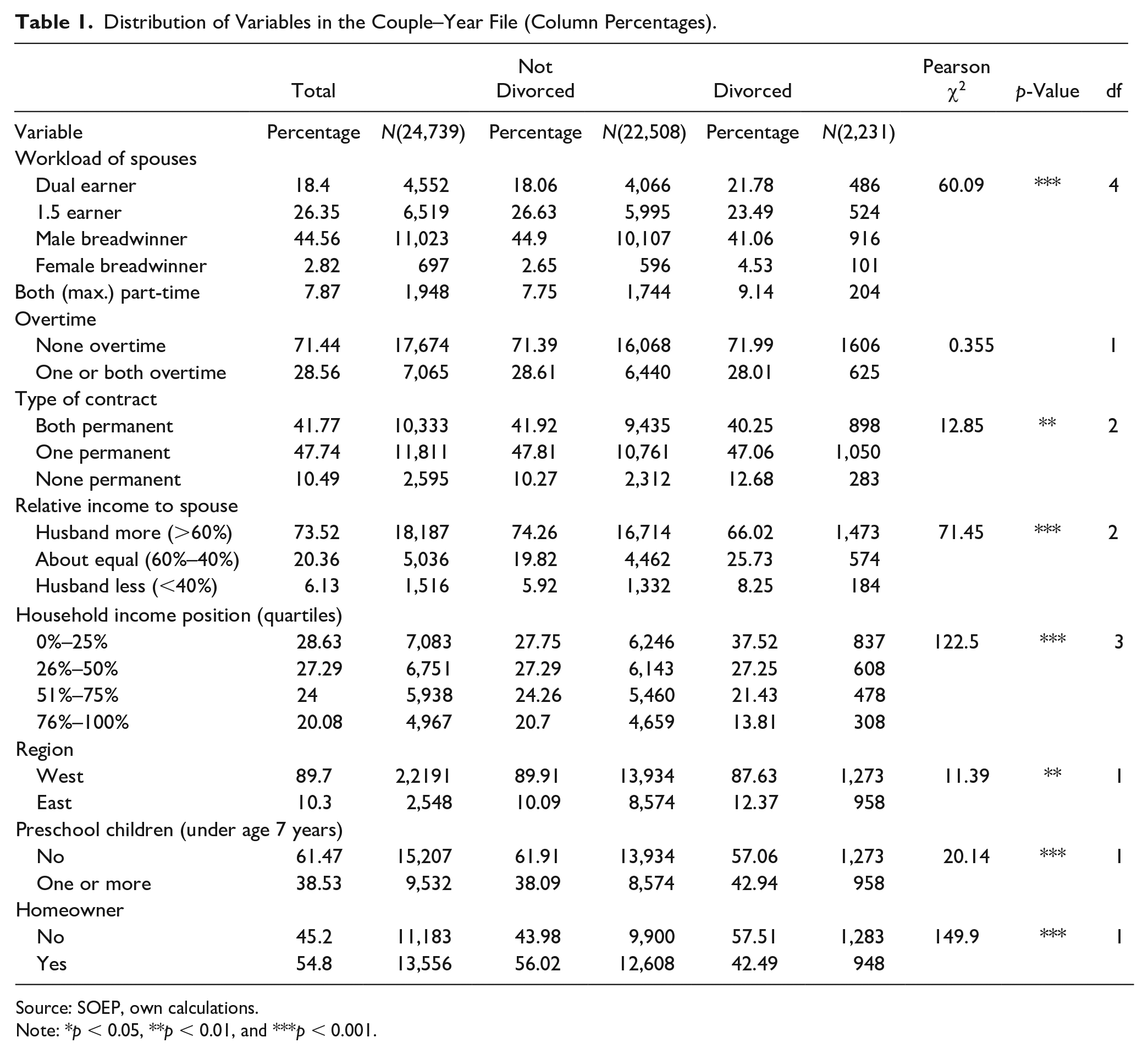
Table 1 shows that in marriages, the most common workload scheme is the traditional one where the husband works full-time and the wife is not employed (42.32%). In 18% of the couples, one spouse is full-time employed and the spouse is part-time employed (1.5 earner), while in 24% of marriages the spouses are dual full-time earners. Uncommon are female breadwinner marriages (3.81%), as well as marriages where both spouses are maximum part-time employed (11.64%). In around 28% of the couples, at least one partner works overtime. The most common combination of contract types are couples where one spouse holds a permanent contract, and the other has no contract or a fixed-term contract (47.18%). Couples where both spouses hold permanent contracts (37.04%) are less common, at about 10%-points. In about 16% of marriages, both spouses hold no permanent contract. The husband earns more than the wife in 67% of the couples, while 25% have earnings that are roughly equal. While 20% of the couples have at least one preschool child, every second couple own their dwellings (51.87%).

Table 1.

Distribution of Variables in the Couple–Year File (Column Percentages).

	Total		Not Divorced		Divorced		Pearson χ²	p-Value	df
Variable	Percentage	N(24,739)	Percentage	N(22,508)	Percentage	N(2,231)
Workload of spouses
Dual earner	18.4	4,552	18.06	4,066	21.78	486	60.09	***	4
1.5 earner	26.35	6,519	26.63	5,995	23.49	524
Male breadwinner	44.56	11,023	44.9	10,107	41.06	916
Female breadwinner	2.82	697	2.65	596	4.53	101
Both (max.) part-time	7.87	1,948	7.75	1,744	9.14	204
Overtime
None overtime	71.44	17,674	71.39	16,068	71.99	1606	0.355		1
One or both overtime	28.56	7,065	28.61	6,440	28.01	625
Type of contract
Both permanent	41.77	10,333	41.92	9,435	40.25	898	12.85	**	2
One permanent	47.74	11,811	47.81	10,761	47.06	1,050
None permanent	10.49	2,595	10.27	2,312	12.68	283
Relative income to spouse
Husband more (>60%)	73.52	18,187	74.26	16,714	66.02	1,473	71.45	***	2
About equal (60%–40%)	20.36	5,036	19.82	4,462	25.73	574
Husband less (<40%)	6.13	1,516	5.92	1,332	8.25	184
Household income position (quartiles)
0%–25%	28.63	7,083	27.75	6,246	37.52	837	122.5	***	3
26%–50%	27.29	6,751	27.29	6,143	27.25	608
51%–75%	24	5,938	24.26	5,460	21.43	478
76%–100%	20.08	4,967	20.7	4,659	13.81	308
Region
West	89.7	2,2191	89.91	13,934	87.63	1,273	11.39	**	1
East	10.3	2,548	10.09	8,574	12.37	958
Preschool children (under age 7 years)
No	61.47	15,207	61.91	13,934	57.06	1,273	20.14	***	1
One or more	38.53	9,532	38.09	8,574	42.94	958
Homeowner
No	45.2	11,183	43.98	9,900	57.51	1,283	149.9	***	1
Yes	54.8	13,556	56.02	12,608	42.49	948

Source: SOEP, own calculations.

Note: *p < 0.05, **p < 0.01, and ***p < 0.001.

The distribution of couples who get divorced at some point in the observational time shows significant differences in comparison to those who do not get divorced on all of the variables except the variable overtime. The final columns of Table 1 show a slightly significant difference between couples staying married and couples breaking up in the variables type of contract of the spouses (χ²(2) = 12.51, p < 0.01) and the regional context (χ²(2) = 11.39, p < 0.01). The distribution of workload of spouses differs significantly between the staying married and the becoming divorced spouses (χ²(4) = 60.09, p < 0.001). The relative income to their spouse and divorce (χ²(2) = 71.45, p < 0.001) as well as the income position of the spouses show a significant difference between the staying married and the divorced in a difference test (χ²(3) = 122.50, p < 0.001), and between homeownership and the marital outcome groups (χ²(1) = 149.90, p < 0.001). Couples with preschool children differ significantly from those couples without preschool children in breaking up their marriage: those spouses with preschool children tend to end their marriage more often (χ²(1) = 20.14, p < 0.001).

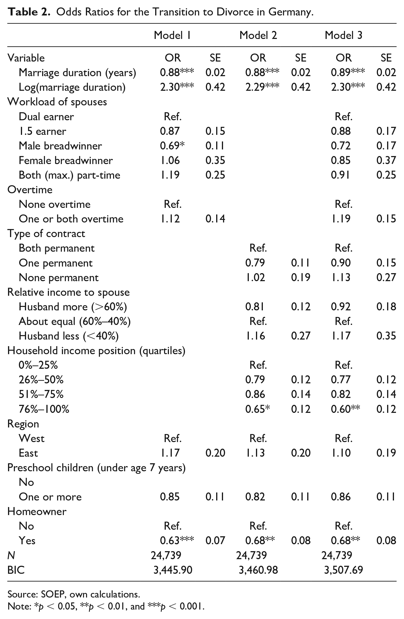
The results of discrete-time event history models on the transition to divorce in Germany are shown in Table 2. Considering the year of marriage in the analysis does not change the results. Therefore, I decided to present models without this variable.

Table 2.

Odds Ratios for the Transition to Divorce in Germany.

	Model 1		Model 2		Model 3
Variable	OR	SE	OR	SE	OR	SE
Marriage duration (years)	0.88***	0.02	0.88***	0.02	0.89***	0.02
Log(marriage duration)	2.30***	0.42	2.29***	0.42	2.30***	0.42
Workload of spouses
Dual earner	Ref.				Ref.
1.5 earner	0.87	0.15			0.88	0.17
Male breadwinner	0.69*	0.11			0.72	0.17
Female breadwinner	1.06	0.35			0.85	0.37
Both (max.) part-time	1.19	0.25			0.91	0.25
Overtime
None overtime	Ref.				Ref.
One or both overtime	1.12	0.14			1.19	0.15
Type of contract
Both permanent			Ref.		Ref.
One permanent			0.79	0.11	0.90	0.15
None permanent			1.02	0.19	1.13	0.27
Relative income to spouse
Husband more (>60%)			0.81	0.12	0.92	0.18
About equal (60%–40%)			Ref.		Ref.
Husband less (<40%)			1.16	0.27	1.17	0.35
Household income position (quartiles)
0%–25%			Ref.		Ref.
26%–50%			0.79	0.12	0.77	0.12
51%–75%			0.86	0.14	0.82	0.14
76%–100%			0.65*	0.12	0.60**	0.12
Region
West	Ref.		Ref.		Ref.
East	1.17	0.20	1.13	0.20	1.10	0.19
Preschool children (under age 7 years)
No
One or more	0.85	0.11	0.82	0.11	0.86	0.11
Homeowner
No	Ref.		Ref.		Ref.
Yes	0.63***	0.07	0.68**	0.08	0.68**	0.08
N	24,739		24,739		24,739
BIC	3,445.90		3,460.98		3,507.69

Source: SOEP, own calculations.

Note: *p < 0.05, **p < 0.01, and ***p < 0.001.

The model on time stress (see model 1, Table 2) provides evidence for a significantly lower divorce risk of marriages, where the husband works full-time, and the wife is not employed compared to dual full-time employed spouses. Although the odds ratios tend to the expected lower dissolution risk in couples with lower workloads, female breadwinner couples and both couples working maximum part-time tend to be less stable as dual-earner couples. However, the results do not show significant changes in marital stability for couples with lower time stress. In other words, marital stability is comparable in couples where both spouses work full-time, female breadwinner marriages, 1.5 earner marriages, and underemployed spouses. Working overtime and living with preschool children are not associated with marital stability, but tendencies are, as expected, higher for couples working overtime and lower for couples having preschool children.

Figure 2 shows the average marginal effects of the interaction of temporal workload of the spouses and preschool children (for b-coefficients, see model 4, Table A2). In other words, it shows the probability to divorce for married couples with preschool children in a given workload group compared to the couples without preschool children with the same workload (x = 0 in Figure 2). An average marginal effect larger than 0 indicates a higher probability to divorce, while an average marginal effect smaller than 0 indicates a lower risk of dissolution. Furthermore, Figure 2 presents the 95% confidence intervals of the average marginal effect. If the confidence interval does not include 0 (reference group), parents of preschool children and parents married without preschool children will differ significantly. The results indicate that the association of workload of spouses and divorce risk does not vary significantly for spouses with and without preschool children. However, dual-earner marriages with preschool children tend to a lower probability to divorce compared to dual-earner marriages without a preschool child. Figure 2 also presents a tendency for a lower probability to divorce in parents with a preschool child in male breadwinner and female breadwinner families (not significantly different). These findings for spouses with and without preschool children remain stable estimating indicators of time stress and financial stress in a joint model (see model 5, Table A2 or Figure A1).

Figure 2.

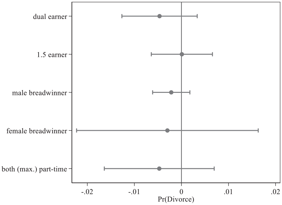
Average marginal effects of divorce and 95% confidence intervals by interaction of temporal workload of the spouses and preschool children (see model 4, Table A2); Reference: no preschool child in the given workload group.

The model testing the financial stress mechanism (see model 2, Table 2) shows a lower risk of divorce for couples with only one spouse holding a permanent contract compared to those marriages where both spouses hold permanent contracts (OR = 0.79, p > 0.05). Couples where none of the spouses hold a permanent contract do not differ from both husband and wife holding a permanent contract. Traditional income structure marriages, indicated by a higher income of the husband compared to his wife, have a lower risk of divorce compared to marriages with equal income. Marriages where the female spouse earns more than the male spouse tend to have a lower marital stability compared to equal income couples. The results for type of contract and relative income to spouse in model 2 do not significantly differ from 0.

However, the income position of the spouses compared to other married couples is associated with marital stability, as expected. The divorce risk differs across social strata, based on incomes. Despite the nonsignificant odds ratios, it is noteworthy that the second and third income quartiles show a slightly lower risk of divorce compared to the first quartile. Couples in the fourth income quartile show significantly lower divorce risk compared to the lowest income quartile marriages. Living in East Germany or West Germany shows no significantly different odds ratios for marital dissolution, but it tends to be positively associated for spouses living in East Germany (OR = 1.13, p > 0.05). Spouses owning a dwelling have significantly lower risk of divorce compared to non-homeowner couples (OR = 0.68, p < 0.01). This finding is in line with previous studies (Lersch & Vidal, 2014; Wagner & Weiß, 2006).

Estimating financial stress and time stress in a joint model, the association of workload on marital stability vanishes, while it remains stabilizing for spouses belonging to the highest income quartile and to own a dwelling. The explanatory power of the full model is worse than that of models 1 and 2 (BIC is highest in the full model, see Table 2). But why do the time stress associations disappear in the full model? Time stress and financial stress seem to be mutually dependent. Thus, the results ask for further information if marriages without financial stress are able to cope with time stress as they may perceive the time stress worthy of their financial gains. A model where workload and income position⁵ interact shows no significant differences between high- and low-income marriages and divorce risk in the different workload groups (see Figure A2). In other words, time stress is not only straining couples that have low financial resources. Furthermore, homeownership seems to blur the relevance of couples income position, as couples in each of the income quartiles tend to have lower risks of divorce compared to married couples in the lowest income quartile, which can be shown in estimating M3 without controlling for homeownership (results not shown).

Discussion and Conclusion

In this study, I set out to investigate whether spouses’ precarious job characteristics have an impact on the stability of their marriage. To answer this question, I outlined the previous research on three dimensions of job characteristics: workload, employment stability, and income. Based on stress theories, I highlight two underlying mechanisms for the association between employment situation and marital stability. Time stress induced by the couples’ workload and financial stress emerging from precarious employment or low income can strain couples, and I set out to derive five hypotheses. Using a discrete-time event history analysis on marriages not older than 1985 from the SOEP data, I shed light on the effects of working hours, working overtime, employment stability, couples’ relative income to their spouse, and their relative income position to other married couples on divorce risk. In modeling dependence on a spouse’s employment situation, I expand previous research that mostly failed to use conjoint information on the employment situation of married couples. Neither in line with previous research detecting a higher marital stability for women working part-time in Germany (e.g., Cooke, 2006) nor with my assumption (H1), I find a lower divorce risk for couples who did perform the male breadwinner model with a husband working full-time and a not employed wife. There is no negative association of working overtime on marital stability, contrasting my assumption that working overtime reduces couples’ leisure time (H1 not accepted). Additionally, I cannot detect a difference of time stress and divorce between parents of preschool children and spouses without preschool children who are assumed to suffer from a higher time stress due to caring obligations (H2 not accepted). Following these results with a dyadic perspective, spouses’ employment situation does not induce as much time stress as spouses’ break up marriages.

Contrary to my assumption, I cannot detect a significant association of the type of contract on divorce risk for couples with nonpermanent contracts compared to couples where both spouses hold permanent contracts (H3). This is not in line with previous research that clearly detects a higher divorce risk for persons in unstable employment situations (Böhm et al., 2010; Kaplan & Herbst, 2015). Couples instead may attenuate for the precarious employment situation of a spouse. This contradicts the theoretical path of uncertain employment situation, producing financial stress, despite the evidence of a higher perceived job insecurity among fixed-term employed couples compared to employees holding a permanent contract (Balz, 2017; Erlinghagen, 2007). Oppenheimer’s argument that couples with equal income have a lower divorce risk than traditional income couples is not supported (H4 not accepted). This finding is not in line with previous research that detects a positive association between female income and divorce (Cooke, 2006; Kalmijn et al., 2007; Kaplan & Herbst, 2015). The couples’ social position in the income hierarchy is a predictor of divorce risk as marriages from the highest income quartile have shown higher marital stability. This is in line with previous research and my derived assumptions (H5 not rejected).

Taking a dyadic perspective into account, financial stress, caused by precarious contracts and its spill-over mechanism, does not fit well in explaining the interplay of employment situation and marital instability. However, my results provide some evidence for the financial stress mechanism in marriages as high-strata couples have lower divorce risk. In this case, selection could play a role, as homeownership also shows a significant reduction in divorce risk. In other words, couples who can afford investments or have high income are less prone to divorce. Or, to put it the other way around, married couples who are more stable make joint investments.

All in all, it appears that it is important to take the dyadic perspective into account in studies pertaining to divorce. There are likely many causal pathways running through spouses’ employment situation that cannot be captured in this article and will require further research. The test of stress mechanisms can be improved in future research in using information on perceived time stress of spouses. Surprisingly, with the objective measurement of time stress, there is no explanatory power of couples’ conjoint job characteristics in terms of workload on divorce risk. However, it seems to be beneficial to follow a traditional division of labor and to invest in marriage by foregoing a full-time career of the female spouse by reducing labor participation to ensure a stable marriage. Otherwise, it could be reverse causation, as couples decide for workload models to avoid time stress, for example if they have preschool children. These couples do not suffer from their workload and perform as per gender norms, which lead to stable marriages. Thus, financial stress partly explains marital instability. This is in line with the Family Stress model and shows the vulnerability of low-income couples who seem to have lower coping resources. Nevertheless, low income does not moderate the association between workload and marital stability.

As long as the SOEP contains information on both partners being directly interviewed, it is possible to employ the analysis on data of good quality. My results do not suffer from recall bias in remembering employment characteristics of positions held long ago, as I only use prospective information for the operationalization of the main predictors and no retrospective data. Also, length bias, which emerges due to left truncated data, does not affect my results as I only analyze couples married in 1985 or later. However, the study has two limitations: (a) the estimations outlined earlier are a rather conservative test of the assumptions outlined previously as I have applied listwise deletion in data processing. Thus, a problem with the data could be that I can only analyze episodes of couples in which both of the spouses responded, leaving a fair amount of missing data points. Missingness is emerging already if at least one spouse of a couple does not provide information on one of the predictor variables. Furthermore, previous research has shown that dissolution is related to panel attrition (Mitchell, 2010; Müller & Castiglioni, 2015), and that survey data tend to underestimate the transition to divorce (Boertien, 2020). Therefore, I assume that the estimations are conservative.

(b) This study takes into account married couples and not cohabiting couples. However, cohabiting couples are a heterogeneous family type (Hiekel et al., 2015) with a lower level of institutionalization than married couples. Studies provide evidence that cohabiting and married couples vary in transitions of the family life course (e.g., Perelli-Harris, 2014, for the transition to second birth). From Finland we know that the role of socioeconomic resources in relationship stability varies between cohabiting and married unions (Jalovaara, 2013). As cohabiting couples can differ with respect to union stability (Kiernan, 2001), it is out of the scope of this article. However, future research should investigate whether job characteristics are related to transitions (dissolution or marriage) in cohabiting couples. As couples who marry despite financial or time stress seem to be special in their stability (as they have “selected” into marriage), we may find evidence for these financial or time stress mechanisms in cohabiting unions.

The common critique on divorce research is that it lacks on couples’ situations as a unit. But concerning employment situation, the couples’ factors do not seem to underline previous research on the risk of divorce. However, the dyadic perspective could be a beneficial approach for other fields of life that may affect marital stability, like norms and attitudes of marital partners. In Germany, stable marriages follow a main earner model and homeownership. Although the German social politics have a long tradition in providing 1.5 earner families, the traditional workload does not stabilize marriages, neither with nor without children. This underlines the importance of changing family benefits, however, the youngest reforms regarding parental allowance (ElterngeldPlus) are a first step towards a more flexible system that supports families with regard to their individual requirements.

Footnotes

Appendix A

Table A2.

Transition to Divorce in Germany, Interaction of Temporal Workload and Children.

	Model 4		Model 5
Variable	b	SE	b	SE
Marriage duration (years)	−0.12***	0.03	−0.12***	0.03
Log (marriage duration)	0.83***	0.18	0.83***	0.18
Workload of spouses
Dual earner	Ref.		Ref.
1.5 earner, male	−0.23	0.20	−0.22	0.22
Male breadwinner	−0.39*	0.20	−0.37	0.27
Female breadwinner	0.04	0.37	−0.18	0.48
Both (max.) part-time	0.18	0.26	−0.09	0.31
Interaction workload of spouses* preschool children
Dual-earner*children (1)	Ref.		Ref.
1.5 earner, male*children (1)	0.34	0.40	0.34	0.40
Male-breadwinner*children (1)	0.14	0.37	0.17	0.37
Female-breadwinner*children (1)	0.13	0.75	0.18	0.75
Both (max.) part-time*children (1)	0.06	0.46	0.07	0.46
Overtime
None overtime	Ref.		Ref.
One or both overtime	0.12	0.13	0.17	0.13
Type of contract
Both permanent			Ref.
One permanent			−0.10	0.17
None permanent			0.13	0.24
Relative income to spouse
Husband more (>60%)			−0.08	0.19
About equal (60%–40%)			Ref.
Husband less (<40%)			0.14	0.29
Household income position (quartiles)
0%–25%			Ref.
26%–50%			−0.26	0.15
51%–75%			−0.20	0.16
76%–100%			−0.50*	0.19
West	Ref.		Ref.
East	0.16	0.17	0.09	0.18
Preschool children (under age 7 years)
No	Ref.		Ref.
One or more	−0.32	0.32	−0.33	0.32
Homeowner
No	Ref.		Ref.
Yes	−0.46***	0.12	−0.38**	0.12
Constant	−4.38***	0.20	−4.16***	0.23
N	24,739		24,739
BIC	3,485.47		3,547.28

Source: SOEP, own calculations.

Note: *p < 0.05, **p < 0.01, and ***p < 0.001.

Declaration of Conflicting Interests

The author declared no potential conflicts of interest with respect to the research, authorship, and/or publication of this article.

Funding

The author received no financial support for the research, authorship, and/or publication of this article.

ORCID iD

Lisa Schmid

Notes

References

Allison

P. D.

(1982). Discrete-time methods for the analysis of event histories. Sociological Methodology, 13, 61–98.

Allison

P. D.

(2014). Event history and survival analysis (2nd ed.). Sage Publications.

Aneshensel

C. S.

(1992). Social stress: Theory and research. Annual Review of Sociology, 18, 15–38.

Balz

(2017). Cross-national variations in the security gap: Perceived job insecurity among temporary and permanent employees and employment protection legislation. European Sociological Review, 33(5), 675–692. https://doi.org/10.1093/esr/jcx067

Becker

G. S.

Landes

E. M.

Michael

R. T.

(1977). An economic analysis of marital instability. Journal of Political Economy, 85(6), 1141–1187.

BiB, Bundesinstitut für Bevölkerungsforschung. (2018). Shares of marriages dissolved of the marriage years 1965, 1975, 1985, 1995 and 2005 by duration of marriage in Germany (as per: 2018) [Anteile der geschiedenen Ehen der Eheschleißungsjahrgänge (1965-2005) nach der Ehedauer in Deutschland (Stand:2018)]. https://www.bib.bund.de/Permalink.html?id=10238144

Blossfeld

H.-P.

Drobnič

Rohwer

(2001). Spouse’ employment career in (West) Germany. In Blossfeld

H.-P.

Drobnič

(Eds.), Careers of couples in contemporary societies. From male breadwinner to dual earner families (pp. 53–76). University Press.

Bodenmann

(1997). Dyadisches coping: Theoretischer und empirischer Stand. Zeitschrift für Familienforschung, 9, 7–25.

Bodenmann

(2009). Stress und Coping bei Paaren. Hofgrefe-Verlag.

10.

Boertien

(2020). The conceptual and empirical challenges of estimating trends in union stability: Have unions become more stable in Britain? In Mortelmans

(Ed.), Divorce in Europe (Vol. 21, pp. 17–36). Springer International Publishing. https://doi.org/10.1007/978-3-030-25838-2_2

11.

Böhm

Diewald

Körnert

(2010). Instabile Partnerschaften durch neue Beschäftigungsformen? Risiken von Männern und Frauen. In Berger

P. A.

Hitzler

(Eds.), Individualisierungen. Ein Vierteljahrhundert „jenseits von Stand und Klasse”? (pp. 211–224). VS Verlag für Sozialwissenschaften.

12.

Böttcher

(2006). Scheidung in Ost- und Westdeutschland: Der Einfluss der Frauenerwerbstätigkeit auf die Ehestabilität. KZfSS Kölner Zeitschrift für Soziologie und Sozialpsychologie, 58(4), 592–616. https://doi.org/10.1007/s11577-006-0258-1

13.

Brenke

(2015). Growing importance of women in the German labor market. DIW Economic Bulletin, 5(5), 51–61.

14.

Brüderl

Engelhardt

(1997). Trennung oder Scheidung? Einige methodologische Überlegungen zur Definition von Eheauflösungen. Soziale Welt, 48(3), 277–289.

15.

Buck

A. A.

Neff

L. A.

(2012). Stress spillover in early marriage: The role of self-regulatory depletion. Journal of Family Psychology, 26(5), 698–708. https://doi.org/10.1037/a0029260

16.

Conger

R. D.

Conger

K. J.

(2002). Resilience in midwestern families: Selected findings from the first decade of a prospective, longitudinal study. Journal of Marriage and Family, 64(2), 361–373. https://doi.org/10.1111/j.1741-3737.2002.00361.x

17.

Conger

R. D.

Conger

K. J.

Martin

M. J.

(2010). Socioeconomic status, family processes,and individual development. Journal of Marriage and Family, 72(3), 685–704. https://doi.org/10.1111/j.1741-3737.2010.00725.x

18.

Cooke

L. P.

(2004). The gendered division of labor and family outcomes in Germany. Journal of Marriage and Family, 66, 1246–1256.

19.

Cooke

L. P.

(2006). “Doing” gender in context: Household bargaining and the risk of divorce in Germany and the United States. American Journal of Sociology, 112(2), 442–472.

20.

Cooke

L. P.

Gash

(2010). Wives’ part-time employment and marital stability in Great Britain, West Germany and the United States. Sociology, 44(6), 1091–1108. https://doi.org/10.1177/0038038510381605

21.

Cooke

L. P.

Erola

Evertsson

Gähler

Härkönen

Hewitt

Jalovaara

Kan

M.-Y.

Lyngstad

T. H.

Mencarini

Mignot

J.-F.

Mortelmans

Poortman

A.-R.

Schmitt

Trappe

(2013). Labor and love: Wives’ employment and divorce risk in its socio-political context. Social Politics: International Studies in Gender, State & Society, 20(4), 482–509. https://doi.org/10.1093/sp/jxt016

22.

Cousins

C. R.

Tang

(2004). Working time and work and family conflict in the Netherlands, Sweden and the Uk. Work, Employment and Society, 18(3), 531–549. https://doi.org/10.1177/0950017004045549

23.

Dietz

Himsel

Walwei

(2013). Wandel der Erwerbsformen: Weche Rolle spielen strukelle Änderungen am Arbeitsmarkt? Arbeit, 22(2), 85–104.

24.

Erlinghagen

(2007). Self-perceived job insecurity and social context: A multi-level analysis of 17 European countries. European Sociological Review, 24(2), 183–197. https://doi.org/10.1093/esr/jcm042

25.

Eurostat. (2016). Divorces in 100 marriages: Divorce Indicators. http://appsso.eurostat.ec.europa.eu/nui/show.do?dataset=demo_ndivind&lang=en

26.

Franzese

Rapp

(2013). Der Einfluss von Arbeitslosigkeit auf das Trennungsrisiko von Ehen. Zeitschrift für Familienforschung, 25(3), 331–345.

27.

Grabka

M. M.

(2016). SOEP 2015—Codebook for the $PEQUIV File 1984-2015: CNEF variables with extended income information for the SOEP (Series D—Variable Description and Coding Nr. 343; SOEP Survey papers). DIW/SOEP. http://panel.gsoep.de/soep-docs/surveypapers/diw_ssp0343.pdf

28.

Hiekel

Liefbroer

A. C.

Poortman

A.-R.

(2015). Marriage and separation risks among German cohabiters: Differences between types of cohabiter. Population Studies, 69(2), 237–251. https://doi.org/10.1080/00324728.2015.1037334

29.

Jalovaara

(2003). The joint effects of marriage partners’ socioeconomic positions on the risk of divorce. Demography, 40(1), 67–81.

30.

Jalovaara

(2013). Socioeconomic resources and the dissolution of cohabitations and marriages. European Journal of Population/Revue Européenne de Démographie, 29(2), 167–193. https://doi.org/10.1007/s10680-012-9280-3

31.

Kalmijn

Loeve

Manting

(2007). Income dynamics in couples and the dissolution of marriage and cohabitation. Demography, 44(1), 159–179.

32.

Kaplan

Herbst

(2015). Stratified patterns of divorce: Earnings, education, and gender. Demographic Research, 32, 949–982. https://doi.org/10.4054/DemRes.2015.32.34

33.

Karabchuk

(2016). The subjective well-being of women in Europe: Children, work and employment protection legislation. Mind & Society, 15(2), 219–245. https://doi.org/10.1007/s11299-016-0194-3

34.

Karney

B. R.

Bradbury

T. N.

(1995). The longitudinal course of marital quality and stability: A review of theory, method, and research. Psychological Bulletin, 118(1), 3–34.

35.

Kiernan

(2001). The rise of cohabitation and childbearing outside marriage in western Europe. International Journal of Law, Policy and the Family, 15(1), 1–21. https://doi.org/10.1093/lawfam/15.1.1

36.

Kreyenfeld

Geisler

(2006). Müttererwerbstätigkeit in Ost- und Westdeutschland. Zeitschrift für Familienforschung, 18(3), 333–360.

37.

Lersch

P. M.

Vidal

(2014). Falling out of love and down the housing ladder: A longitudinal analysis of marital separation and home ownership. European Sociological Review, 30(4), 512–524. https://doi.org/10.1093/esr/jcu055

38.

Lewis

(1992). Gender and the development of welfare regimes. Journal of European Social Policy, 2(3), 159–173. https://doi.org/10.1177/095892879200200301

39.

Lyngstad

Jalovaara

(2010). A review of the antecedents of union dissolution. Demographic Research, 23, 257–292. https://doi.org/10.4054/DemRes.2010.23.10

40.

Mau

Mewes

Schöneck

N. M.

(2012). What determines subjective socio-economic insecurity? Context and class in comparative perspective. Socio-Economic Review, 10(4), 655–682. https://doi.org/10.1093/ser/mws001

41.

Mitchell

(2010). Are divorce studies trustworthy? The effects of survey nonresponse and response errors. Journal of Marriage and Family, 72(4), 893–905. https://doi.org/10.1111/j.1741-3737.2010.00737.x

42.

Müller

Castiglioni

(2015). Attrition im Beziehungs- und Familienpanel pairfam. In Schupp

Wolf

(Eds.), Nonresponse Bias (pp. 383–408). Springer Fachmedien Wiesbaden. https://doi.org/10.1007/978-3-658-10459-7_12

43.

Niehaus

(2012). Leiharbeit und Privatleben: Auswirkungen einer flexiblen Beschäftigungsform auf Partnerschaft und Familie. Berliner Journal für Soziologie, 22(4), 569–594. https://doi.org/10.1007/s11609-012-0199-7

44.

OECD. (2014). Part-time employment rate. OECD Publishing. https://doi.org/10.1787/f2ad596c-en

45.

Oppenheimer

V. K.

(1997). Women’s employment and the gain to marriage: The specialization and trading model. Annual Review of Sociology, 23, 431–453.

46.

Ostner

Lewis

(1995). Gender and the evolution of European social policies. In Leibfried

Pierson

(Eds.), European Social Policy. Between Fragmentation and Integration (pp. 159–193). Brookings Institution.

47.

Özcan

Breen

(2012). Marital instability and female labor supply. Annual Review of Sociology, 38(1), 463–481. https://doi.org/10.1146/annurev-soc-071811-145457

48.

Perelli-Harris

(2014). How similar are cohabiting and married parents? Second conception risks by union type in the United States and across Europe. European Journal of Population, 30(4), 437–464. https://doi.org/10.1007/s10680-014-9320-2

49.

Poortman

A.-R.

(2005a). How work affects divorce: The mediating role of financial and time pressures. Journal of Family Issues, 26(2), 168–195. https://doi.org/10.1177/0192513X04270228

50.

Poortman

A.-R.

(2005b). Women’s work and divorce: A matter of anticipation? A research note. European Sociological Review, 21(3), 301–309. https://doi.org/10.1093/esr/jci019

51.

Raeymaeckers

Snoeckx

Mortelmans

Van Ourti

(2006). Marriage and divorce in Belgium: The influence of professional, financial and educational resources on the risk for marriage dissolution. Journal of Divorce & Remarriage, 46(1–2), 151–174. https://doi.org/10.1300/J087v46n01_09

52.

Randall

A. K.

Bodenmann

(2009). The role of stress on close relationships and marital satisfaction. Clinical Psychology Review, 29(2), 105–115. https://doi.org/10.1016/j.cpr.2008.10.004

53.

Randall

A. K.

Bodenmann

(2017). Stress and its associations with relationship satisfaction. Current Opinion in Psychology, 13, 96–106. https://doi.org/10.1016/j.copsyc.2016.05.010

54.

Rogers

S. J.

(2004). Dollars, dependency, and divorce: Four Perspectives on the role of wives’ income. Journal of Marriage and Family, 66(1), 59–74. https://doi.org/10.1111/j.1741-3737.2004.00005.x

55.

Ruggles

(1997). The rise of divorce and separation in the Unitd States, 1880–1990. Demography, 34(4), 455. https://doi.org/10.2307/3038300

56.

Schoen

Astone

N. M.

Rothert

Standish

Kim

Y. J.

(2002). Women’s employment, marital happiness, and divorce. Social Forces, 2(81), 643–662.

57.

Schulz

M. S.

Cowan

P. A.

Pape Cowan

Brennan

R. T.

(2004). Coming home upset: Gender, marital satisfaction, and the daily spillover of workday experience into couple interactions. Journal of Family Psychology, 18(1), 250–263. https://doi.org/10.1037/0893-3200.18.1.250

58.

Schupp

Goebel

Kroh

Schröder

Bartels

Erhardt

Fedorets

Grabka

Giesselmann

Krause

Kuehne

Richter

Siegers

Schmelzer

Schmitt

Schnitzlein

Wenzig

Research

G. I. F. E

. (2017). Socio-economic Panel (SOEP), data from 1984-2015. SOEP Socio-Economic Panel Study. https://doi.org/10.5684/soep.v32.1

59.

Singer

J. D.

Willett

J. B.

(2003). Applied longitudinal data analysis: Modeling change and event occurrence. Oxford University Press.

60.

South

S. J.

(2001). Time-dependent effects of wives’ employment on marital dissolution. American Sociological Review, 66(2), 226–245.

61.

Steele

Kallis

Goldstein

Joshi

(2005). The relationship between childbearing and transitions from marriage and cohabitation in Britain. Demography, 42(4), 647–673. https://doi.org/10.1353/dem.2005.0038

62.

Story

L. B.

Bradbury

T. N.

(2004). Understanding marriage and stress: Essential questions and challenges. Clinical Psychology Review, 23(8), 1139–1162. https://doi.org/10.1016/j.cpr.2003.10.002

63.

Teachman

(2010). Wives’ economic resources and risk of divorce. Journal of Family Issues, 31(10), 1305–1323. https://doi.org/10.1177/0192513X10370108

64.

TNS Infratest Sozialforschung. (2015). SOEP 2015- Erhebungsinstrumente 2015 (Welle 32) des Sozio-oekonomischen Panels: Haushaltsfragebogen Altstichproben (SOEP Survey Papers, Nr. 274-Series A). DIW/SOEP.

65.

Trappe

Pollmann-Schult

Schmitt

(2015). The rise and decline of the male breadwinner model: Institutional underpinnings and future expectations. European Sociological Review, 31(2), 230–242. https://doi.org/10.1093/esr/jcv015

66.

van Damme

Kalmijn

. (2014). The dynamic relationships between union dissolution and women’s employment: A life-history analysis of 16 countries. Social Science Research, 48, 261–278. https://doi.org/10.1016/j.ssresearch.2014.06.009

67.

Wagner

G. G.

Göbel

Krause

Pischner

Sieber

(2008). Das Sozio-oekonomische Panel (SOEP): Multidisziplinäres Haushaltspanel und Kohortenstudie für Deutschland – Eine Einführung (für neue Datennutzer) mit einem Ausblick (für erfahrene Anwender). AStA Wirtschafts- und Sozialstatistisches Archiv, 2(4), 301–328. https://doi.org/10.1007/s11943-008-0050-y

68.

Wagner

Weiß

(2003). Bilanz der deutschen Scheidungsforschung. Versuch einer Meta-Analyse. Zeitschrift für Soziologie, 32(1), 29–49.

69.

Wagner

Weiß

(2006). On the variation of divorce risks in Europe: Findings from a meta-analysis of European longitudinal studies. European Sociological Review, 22(5), 483–500. https://doi.org/10.1093/esr/jcl014

70.

Wagner

Weiß

(2010). Erwerbssituation und Partnerschaft: Deutsche und türkische Paare im Vergleich. In Beckers

Birkelbach

Hagenah

Rosar

(Eds.), Komparative empirische Sozialforschung (pp. 169–198). VS Verlag für Sozialwissenschaften.

71.

Wagner

Schmid

Weiß

(2015). Exploring increasing divorce rates in West Germany: Can we explain the iron law of increasing marriage instability? European Sociological Review, 31(2), 211–229. https://doi.org/10.1093/esr/jcv014

Spouses’ Employment Situations and Marital Separation in Germany: A Dyadic Perspective

Abstract

Keywords

Introduction

Background

Workload and Divorce

Employment Stability, Income, and Divorce

Materials and Methods

Data

Outcome Variable

Predictor Variables

Method

Results

Discussion and Conclusion

Footnotes

Appendix A

Declaration of Conflicting Interests

Funding

ORCID iD

Notes

References