Sage Journals: Discover world-class research

Abstract

Thermal treatments that use ultrasound devices as a tool have as a key point the temperature control to be applied in a specific region of the patient’s body. This kind of procedure requires caution because the wrong regulation can either limit the treatment or aggravate an existing injury. Therefore, determining the temperature in a region of interest in real-time is a subject of high interest. Although this is still an open problem, in the field of ultrasound analysis, the use of machine learning as a tool for both imaging and automated diagnostics are application trends. In this work, a data-driven approach is proposed to address the problem of estimating the temperature in regions of a B-mode ultrasound image as a supervised learning problem. The proposal consists in presenting a novel data modeling for the problem that includes information retrieved from conventional B-mode ultrasound images and a parametric image built based on changes in backscattered energy (CBE). Then, we compare the performance of classic models in the literature. The computational results presented that, in a simulated scenario, the proposed approach that a Gradient Boosting model would be able to estimate the temperature with a mean absolute error of around 0.5°C, which is acceptable in practical environments both in physiotherapic treatments and high intensity focused ultrasound (HIFU).

Keywords

ultrasound imaging B-mode images temperature estimation supervised learning machine learning

Introduction

Thermotherapy consists of a group of treatments that are based on the temperature variation of tissues, encapsulating procedures that work both with the reduction of temperature (using ice or cold air, for example) and those that aim to increase the temperature (using hot water bags or towels, among others).¹ The applications mentioned act, in general, only superficially. To reach deeper tissues, other techniques are necessary. When it comes to temperature increase, heat can be obtained from the use of infrared radiation or ultrasound.

Ultrasound is characterized as any mechanical vibration with a frequency greater than 20 kHz.² In medicine, ultrasound devices are commonly associated with image diagnosis, but the use of therapeutic ultrasound for treating injuries or certain types of cancer has wide application due to its low cost and because it is a harmless and non-invasive procedure.³

Among the existing thermal therapies that use ultrasound as a heat source, hyperthermia is particularly prominent. It is a thermal treatment for some kinds of cancer, where the region is heated to temperatures close to 45°C, which improves the effectiveness of procedures like radiotherapy.⁴ Ultrasound is also used in physiotherapeutic treatments. It is applied, for example, to treat inflammatory conditions by increasing the blood flow and accelerating healing processes.⁵

Being a treatment that requires a specific temperature window to work and since heat does not spread equally, online temperature tracking is an essential procedure. The treatment would be ineffective if the temperature is below the required range. On the other hand, reaching higher temperatures could be harmful, causing burns and undesired effects.

However, tracking the temperature in deep tissues is a particular challenge. The gold standard for measuring the temperature is through invasive techniques using sensing probes, specifically sensors like thermocouples that need to be in direct contact with the region.⁶ This type of procedure is not always a viable option, which leads to an investigation of non-invasive techniques for temperature monitoring, and Magnetic Resonance Thermography (MRT) is presented as an alternative. It is a nonionizing procedure that can retrieve information that is clinically accepted but has major drawbacks, like high-cost and the difficulty to design systems that are not affected by the scanner’s magnetic field.⁷

Non-invasive temperature estimation using ultrasound has been reportedly studied by previous works that have investigated how features of raw ultrasound signals correlate to temperature changes. In Simon et al.,⁸ Anand and Kaczkowski,⁹ the authors show how echo is impacted by temperature changes, while Amini et al.¹⁰ analyzes how ultrasound frequency shifts. More recent works on this subject aim to reach low error rates that can be paired with the ones provided by MRI (0.5ºC).¹¹ In Ferreira et al.¹², the authors present a non-invasive method based on the usage of a b-spline neural network for estimating the temperature variation using an artificial tissue. Alvarenga et al.¹³ describes a method for evaluating the variations in the gray levels generated by changes in temperature, as these changes affect the backscattered ultrasound signal.

Backscattered energy is an acoustic property that is commonly used to estimate temperature. It is the portion of the energy that travels back to the transducer after it interacts with a medium or an object. Other works aimed at studying the impact of changes in backscattered energy (CBE). In Straube and Arthur.¹⁴ the authors demonstrate how the power of backscattered ultrasound is dependent on temperature. Arthur et al.¹⁵ present analysis where CBE varies monotonically depending on the medium type, and Shaswary et al.¹⁶ produced 2D temperature maps based on echo shifts and CBE of acoustic harmonic in the temperature range of hyperthermia.

Machine learning (ML) rises as a potential candidate in many domains - including healthcare - when talking about automatic methods to process both structured and unstructured data. From supporting prognosis¹⁷ to highlighting hidden patterns in medical imaging generation¹⁸, the application of artificial intelligence algorithms and usage of intelligent agents has reportedly enhanced both productivity and quality not only in the medical domain but in various sectors of the modern society. Machine learning methods are usually applied to image processing tasks when dealing with ultrasound. In Liu et al.¹⁹ the authors present a literature review showing applications on image classification (the system must decide whether the image belongs to a class or not), image detection (discover if and where the desired element is present in the image), image segmentation (isolate parts of the image that correspond to distinguished elements) and 3D ultrasound analysis. Maraci et al.²⁰ describes an application on obstetrics in which a classification system based on support vector machines is used to detect fetal presentation by analyzing features extracted from images. Zhang et al.²¹ shows a deep neural network to reconstruct ultrasound images from radio-frequency data.

In this work, we seek to model the estimation of the temperature variation on B-mode images as a supervised learning problem. We propose transforming the image information into a structured tabular format that enables the use of machine learning models to estimate variation in a non-invasive way. We resort to the use of a parametric image built based on CBE, which is a novel application for this method.

Material and Methods

Phantom

In the experiments, a digital phantom was used as shown in Figure 1, which consists of a set of concentric rings, where the inner circle and the second ring (white pixels) simulate muscle tissue, and the first and third rings simulate lipid tissue (black pixels). This structure is immersed in an aqueous medium (gray region). The phantom’s dimension is 20mm x 20mm (height x thickness). Figure 2 illustrates the generated B-mode images that represent different temperatures in the range of 37-45ºC. The authors of Teixeira et al.²⁴ generated and provided both the phantom and the temperature images of this simulation using the k-Wave open source MATLAB toolbox.²²

Figure 1.

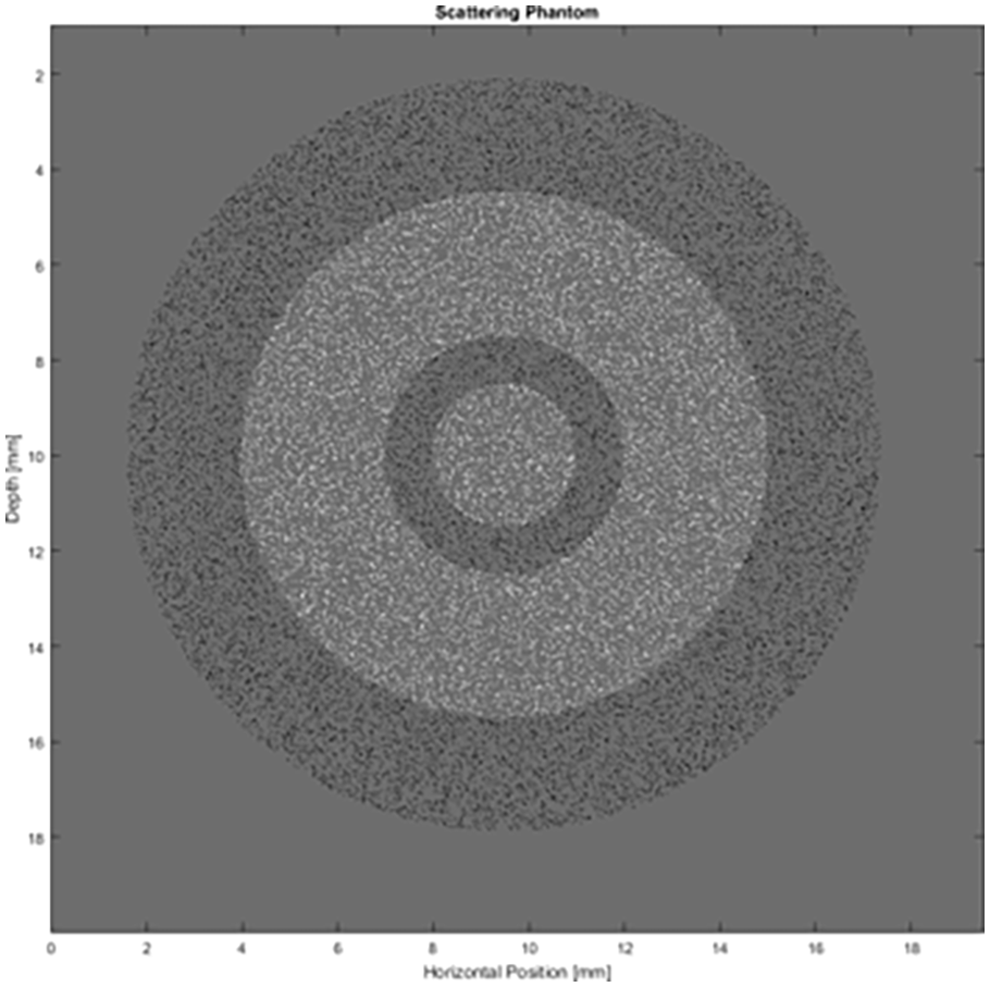
Digital phantom used for B-mode image generation. White pixels simulate muscle tissue, black pixels simulate lipid tissue (fat), and the gray region simulates water. This figure is based on the one presented in Teixeira et al.²⁴

Figure 2.

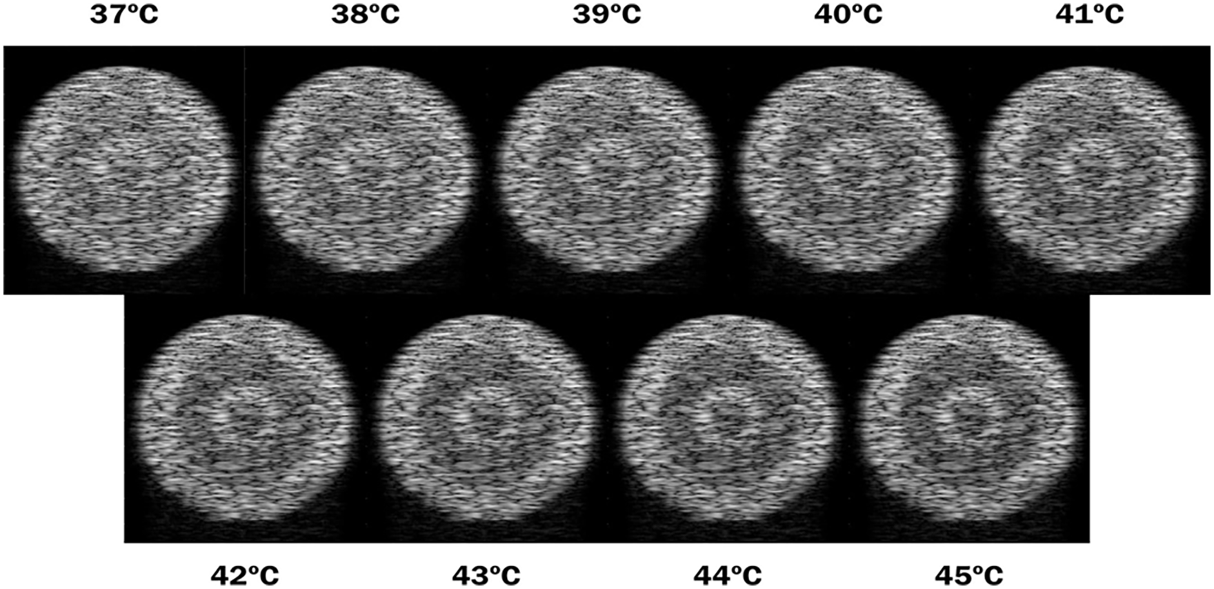
Collection of the resulting B-mode images representing different temperatures obtained using the numeric phantom. In each figure, the related temperature is the same across the whole image.

In Vitro

The experiments were also performed using B-mode ultrasound images generated from in vitro samples of porcine muscle tissue used in Rigueira et al.²³ In this work, the authors aimed to analyze the required dimensions of the region of interest within an image where the contrast generated by the CBEUS image can be visualized by an observer.

The sample was placed in a heat bath in a PVC chamber with water heated by a copper tube. An Ultrasonix SonixMDP scanner with an Ultrasonix L14-5/38 linear transducer was used for generating the B-mode images, while the video capture was performed using the CamStudio software.

First, the sample was maintained at a temperature of 36ºC for 30 minutes to achieve thermal equilibrium. Then, a 30fps video of 5 seconds was recorded. Next, the authors increased the system temperature by 1ºC, maintained the sample at this configuration for 5 minutes, and recorded another 5-second video. The process was repeated until it reached the final temperature of 45ºC.

Figure 3 illustrates B-mode images generated from this sample. Similarly, in the simulation case, a collection of images representing different temperatures in a certain range was used, but in this scenario, we start with a base image at 36ºC up to 45ºC. It is worth mentioning that the B-mode images for each temperature are similar to each other and one cannot detect temperature differences by visual inspection. In this sense, we choose to display only the first and the last images.

Figure 3.

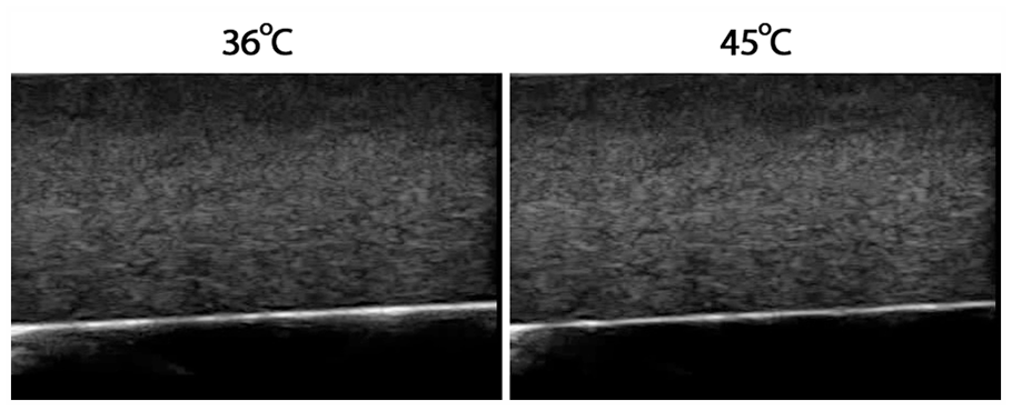
Resulting B-mode images representing temperatures of 36ºC and 45ºC obtained using in vitro porcine skeletal striated muscle. In each figure, the related temperature is the same across the whole image. We use different images for all integer temperature values between the ones displayed in the figure, but they do not present significant differences visually and were omitted for simplification purposes.

CBEUS

In Teixeira et al.¹⁷ the authors explore a new imaging modality in the analysis of intensity changes of pixels related to temperature changes. The novel method proved to be efficient not only by maintaining the ability to distinguish structures but also by providing the identification of new ones.

The method initially takes an ultrasound video recorded at 30 frames per second and generates images averaged in each 5 seconds. By the end of this process, the data is a set of images where each image is the representation of a specific temperature. Since all images have the same resolution, for every pixel p_i×j it is possible to retrieve an array with the grayscale value of all B-mode images. The procedure consists in, for each array of pixels, computing a first-order polynomial that approximates the pixels’ values. Then, for each first-order polynomial retrieve the slope parameter. Finally, a new image is generated by inserting the slope at the corresponding pixel and normalizing the values into the interval [0, 255]. The value of the slope indicates whether the intensity increases or decreases over the temperature variation. Figure 4 illustrates the steps for generating the CBEUS image.

Figure 4.

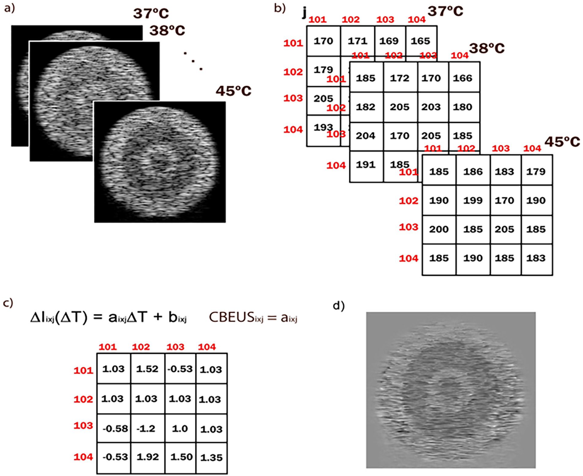
Process for creating a CBEUS image. (a) set of images ordered by temperature level in ascending order. (b) small section of the images with grayscale values of the pixels. (c) the resulting slope parameters for each pixel in the parametric image. (d) the final CBEUS image obtained after pixel value normalization.

In Teixeira et al.²⁴ the authors explore a new imaging modality in the analysis of intensity changes of pixels related to temperature changes, referred to as CBE-based Ultrasound (CBEUS) Imaging. The novel method proved to be efficient not only by maintaining the ability to distinguish structures but also by providing the identification of new ones. During the analysis, the authors noticed that the behavior during heating of a single pixel location could be fit by a linear model and that the angular coefficient (slope parameter) of the linear model was different according to the type of tissue. So, by mapping the angular coefficient, it would be possible to describe the different tissue compositions.

The general process for creating a CBEUS image uses a set of B-mode ultrasound images ordered by temperature level in ascending order. For each pixel location (i, j), the linear model is used to fit the pixel values across all images:

Δ l_{i \times j} (Δ T) = a_{i \times j} Δ T + b_{i \times j}

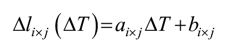
where ΔI_i×j(ΔT ) is the temperature-dependent intensity change for some pixel (i, j), ΔT is the temperature change measured, and ai×j and bi×j are the linear model parameters for pixel (i, j). Then, from the fitted polynomial, the slope parameter a_i×j is retrieved and placed in the same pixel (i, j) of the parametric image. Finally, the CBEUS image is generated after normalizing the pixel values into the interval [0, 255]. Figure 4 illustrates this process.

For clarification purposes, we present three examples of actual values in the experiment with the digital phantom. We choose pixel locations from each of the different tissue type regions. For the muscle tissue region, we retrieve the array [65, 59, 56, 52, 49, 49, 48, 44, 40]. By fitting the first-order polynomial, the model ŷ = −2.73x + 62.27 was obtained, where the slope parameter is −2.73. Next, for the lipid tissue region, we retrieve the array [87, 87, 90, 93, 96, 96, 93, 101, 93]. Similarly, the model ŷ = 1.25x + 87.89 is obtained, with the slope parameter as 1.25. Finally, for the water medium region, we can resort to the external region where the temperature images contain black pixels. The retrieved array should be [0, 0, 0, 0, 0, 0, 0, 0, 0], and the model would be ŷ = 0, and the slope parameter is 0.

The slope parameters are placed in the corresponding pixel locations of the CBEUS image, and the normalization process is applied. In this sense, the lowest value in the matrix will be converted to 0 (black) and the highest value will be converted to 255 (white). As shown in Figure 4d, the muscle region is darker, which relates to the fact that this type of tissue presented a negative slope parameter, i.e. pixels get darker (pixel values get lower) as the temperature rises.

Data Modeling

The modeling starts by considering the following practical scenario: the ultrasonic transducer is applied to the surface of some system, generating a base image that represents the system at a given temperature T₁. After some time, as the heating process occurs, the system temperature raises, and the generated image now represents the same system at a new given temperature T₂. In this practical scenario, we have two images and the desire to estimate the difference ∆ = T2 − T1.

Images are a type of unstructured data, and it is necessary to define a set of processes to extract information to produce features. Since images are a collection of pixels, and there is a direct relation between pixel <i, j> of images T₁ and T₂ if, and only if, the transducer position was not altered during the process, we can track how the pixel value was affected by the temperature variation.

Although the raw pixel value can be used, we also propose the usage of the CBEUS image information in order to incorporate the structure description capability of the parametric image. For generating the CBEUS image it is considered that we have a collection containing n images that are ordered by the referenced temperature. Hence, this collection can be represented as a set

C = {T_{1}, T_{2}, ..., T_{n}}

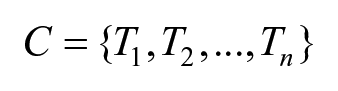
For the sake of the algorithm, n must be at least 2, as the computation of a first order polynomial demands at least two points. In this sense, for a given collection c containing n images, a group g containing n − 1 sets {S₁, S₂, . . ., S_n−₁} can be generated so that:

S₁ contains n − 1 CBEUS images computed using two images with ∆ = 1

S₂ contains n − 2 CBEUS images computed using three images with ∆ = 2

. . .

S_n−₁ contains 1 CBEUS image computed using n images with ∆ = n − 1

Figure 5 illustrates the possible combinations that can be obtained using the simulation images.

Figure 5.

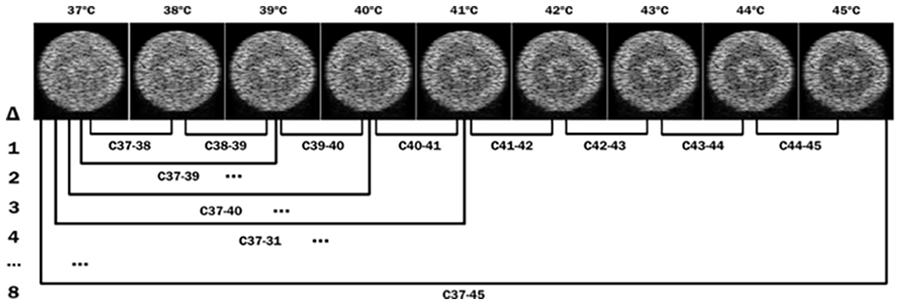
Illustration of the possible arrangements for generating CBEUS images from a set of B-mode images ordered by represented temperature.

By recalling collection C, for each base image a set of CBEUS images with their respective ∆ values were generated. The approach taken was to extract the grayscale values of both images within a certain neighborhood of size n, reshape it in the form of a vector and associate it to the known ∆. Figure 6 illustrates this process. Since the thermal expansion of tissues may lead to a situation where each pixel does not represent the same site in the structure, this procedure is also convenient to account for any pixel displacement caused by temperature rise.

Figure 6.

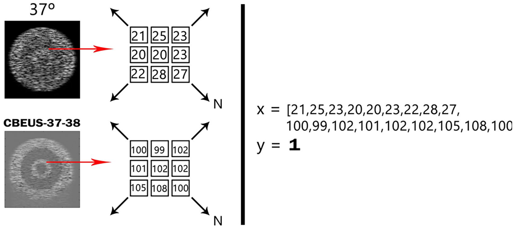
Pictorial representation of the data modeling approach used. By considering a B-mode temperature image and the CBEUS image computed with a certain temperature variation, for the same pixel of both images a neighborhood of size N is selected to generate an observation to the dataset. The expected output of the dataset is the given ∆. The process is repeated for all valid pixels in both images. A valid pixel implies that the neighborhood of size N can be retrieved, that is, it is within the image bounds.

By iteratively performing this process through all viable pixels within all images, a dataset is generated. It must be stated that the dataset is unbalanced, as the sets within collection C presents a different number of images. In this sense, it can be stated that there is a group of observations with a set of known expected outputs and that there are new observations with a similar structure that require the estimation of this output, which is the definition of a supervised learning problem.

Machine Learning Models

After generating the dataset from the images it is possible to feed the data to a supervised machine learning model. In this section, we briefly describe the models used in the experiments and also present arguments that justify the use of these models. On the other hand, the explorations of other models performances should be addressed in future works.

Gradient-boosted decision trees

Decision Trees (DT) are classic machine learning models that generate a classification or predict continuous values by analyzing the input data and trying to create a series of nodes based on Boolean questions.²⁵ Its algorithm aims to produce a tree with the least number of nodes that can correctly decide the outputs. The Gradient-boosted Decision Trees (GBDT) model is an extension of classic DTs.²⁶ It is an ensemble model, i.e. it is composed of a set of simple shallow DTs referred to as weak learners (also called estimators) that work together aiming for producing a better quality prediction. In this work, we resort to a particular implementation of the GBDT model which is part of the XGBoost library.²⁷

GBDT, as implied by its name, uses a technique known as boosting.²⁸ This is one of the possible techniques used by ensemble models to direct how the weak learners are trained. The idea is to add new DTs to the ensemble as the previous DTs are trained, and these new models are focused on correcting the errors generated by the previous learners. The process of minimizing the error within the new models is associated with the idea of the gradient descent algorithm, where we use a learning rate η to define the contribution of each new estimator. The smaller the learning rate, the less the next learner will adapt to previous errors.

Deep neural networks

Deep Learning stands as the current basis for modern artificial intelligence systems, as it has been applied to a wide range of domains reaching state-of-the-art results for applications like image recognition,²⁹ voice generation³⁰ and speech recognition.³¹ This comes from the ability of deep neural models to detect and learn non-linear patterns from data.

A neural network is a classic machine learning model that aims to mimic a living brain.³² It is composed of several elements known as neurons that are units of computation with a series of weights associated with its inputs and an activation function that generates an output. In a neural network, a set of neurons is organized in the shape of layers. Typically, a Deep Neural Network (DNN) is classified as a neural network with at least two hidden layers. Neural networks learn from data through the use of the backpropagation algorithm, in which the data is presented to the network and, after a validation process, the weights are updated to better suit the predictions. As the number of layers rises, the more powerful the network becomes. But this comes with the downside of demanding more time to adjust the weights. The capability of DNN’s is better explored by using of graphics processing units (GPU), which can perform numerous computations in parallel, allowing the distribution calculations involved in the network training process, accelerating this, which is its most computationally costly stage.

An important step in the construction of the topology of a DNN includes the adjustment of the regularization and normalization mechanisms that will be used in it. In this sense, two important parameters are the Batch Normalization,³³ which is the process of normalizing the inputs in the network layers so that the optimization process can be improved, and the Dropout Rate,³⁴ which is the probability of a neuron to be deactivated during the training phase.

Weightless neural networks

Unlike classic neural models such as feedforward or recurrent networks, weightless neural networks (WNN) do not have weights that need to be adjusted using algorithms like gradient descent, thus making its training process faster.³⁵ The most famous weightless neural network model is the WiSARD (Wilkie, Stonham, and Aleksander Recognition Device), which was first used to detect handwritten letters and digits in manuscripts.³⁶ This model uses RAM-like structures as nodes, containing binary addresses that store the number of times that address is accessed. For each class in the problem domain, WiSARD stores a set of RAM nodes in the form of a discriminator that is responsible for recognizing patterns of that class. Besides lower training time, models like WiSARD present a structure that can be directly implemented at a hardware level, which makes them suitable for highperformance and low-power embedded applications^{37, 38}.

As mentioned, the classic WiSARD model is associated with classification problems. An extension of this model known as Regression-WiSARD (ReW) was presented in Lusquino et al.³⁹ so that the RAM-structure nodes could be applied to problems that require the prediction of a continuous value. The main difference between the two models are i) ReW has only one set of RAM nodes and ii) each binary address in the RAM nodes stores another value, which is the sum of the expected values for the patterns presented that access the binary address. The output of the network is the computation of an average measure of the sum returned by each RAM node.

As mentioned, this group of models expects a binary input to be presented, but that is not generally the case. In fact, most data handled in the field of machine learning and data analysis is either in the form of numbers (integer or decimal) and text. So, a binarization process is required so that the data can be transformed. In the context of numeric values, a common approach is to use a technique known as thermometer encoding, where we use the minimum and maximum observed values of a given feature and split this range into t bits (the thermometer size). Initially, we generate a binary word containing t bits 0. Then, for a given value to be converted, we verify where within the specified range the value is placed. All bits that appear before the value are set to 1, so the closest the given value is to the maximum, the more bits 1, and the closest to the minimum, the more bits 0.

Computational Environment

The experiments were developed using the Python3 programing language and the numpy, sklearn⁴⁰, xgboost, TensorFlow modules. All experiments were performed using a system consisting of an AMD Ryzen 7 5700G processor, 32 GB of RAM, NVidia GTX 980 Ti, and Windows 11 operating system.

Results

In this section, we present the results of the performed experiments. The value of the neighborhood N was chosen empirically after experimenting with a set of predefined values [1, 2, 3, 4, 5]. The size of N causes a direct impact on several aspects of the experiment, including dataset size and prediction performance, and N = 5 presented the best scenario.

For each model, a train/test split of the dataset was performed, with 30% of the data reserved for model testing, which comprises the reported results. The process was repeated 10 times and the average of the Mean Absolute Error (MAE) and Mean Squared Error (MSE) metrics were measured. The standard deviation is associated with each value. For both metrics, the closer the reported value is to 0.0, the better.

Table 1 shows the hyperparameters and configurations used in each of the models. These parameter values were obtained empirically, where a finite set of different values was tested, and these configurations returned the best results so far. In the final section, we discuss the necessity of further hyperparameter exploration.

Table 1.

Models’ Parameters That Returned the Best Results Across the Computational Experiments.

Model	Parameters	Explored Values	Best Value
GBDT	η max depth#estimators	0.1, 0.3, 0.53, 6, 1010, 100, 1000	0.361000
DNN	Dropout Rate Batch normalization Epochs	10%, 30%Yes, No10, 20, 100	30%Yes100
ReW	ThermometerAddress sizeMean	5, 10, 202, 4, 8, 16, 32Simple, Median, Exponential	1032Median

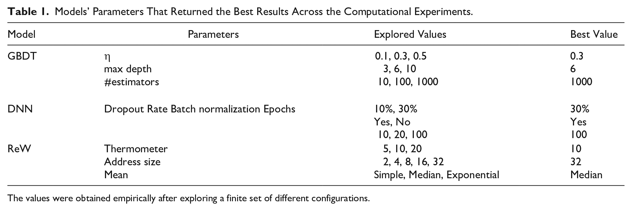
The values were obtained empirically after exploring a finite set of different configurations.

Simulated Data Temperature Estimation

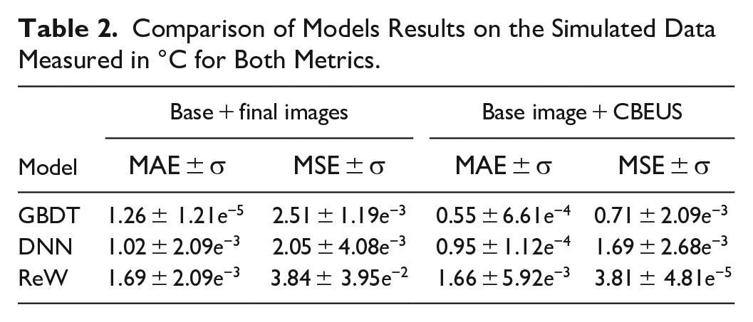
Table 2 shows the comparative results between the models applied to the simulation data. As can be observed, the GBDT algorithm could reach a mean absolute difference of almost 0.5°C. Both DNN and WNN architectures could not reach such difference, with errors above 1.0°C. When observing the MSE it is possible to detect that GBDT remains close to the absolute error, implying that the mispredictions are not far from the expected values.

Table 2.

Comparison of Models Results on the Simulated Data Measured in °C for Both Metrics.

	Base + final images		Base image + CBEUS
Model	MAE ± σ	MSE ± σ	MAE ± σ	MSE ± σ
GBDT	1.26 ± 1.21e⁻⁵	2.51 ± 1.19e⁻³	0.55 ± 6.61e⁻⁴	0.71 ± 2.09e⁻³
DNN	1.02 ± 2.09e⁻³	2.05 ± 4.08e⁻³	0.95 ± 1.12e⁻⁴	1.69 ± 2.68e⁻³
ReW	1.69 ± 2.09e⁻³	3.84 ± 3.95e⁻²	1.66 ± 5.92e⁻³	3.81 ± 4.81e⁻⁵

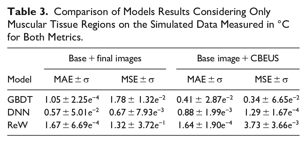
From a general perspective, it is important to emphasize that the data is randomly split, which causes the model to predict pixels related to different tissue types. Table 3 shows the results of predictions applied only to pixels within the region related to muscle tissue. All models’ prediction performance increase, with GBDT reaching values below 0.5°C when considering MAE and presenting even smaller MSE, which indicates smaller errors.

Table 3.

Comparison of Models Results Considering Only Muscular Tissue Regions on the Simulated Data Measured in °C for Both Metrics.

	Base + final images		Base image + CBEUS
Model	MAE ± σ	MSE ± σ	MAE ± σ	MSE ± σ
GBDT	1.05 ± 2.25e⁻⁴	1.78 ± 1.32e⁻²	0.41 ± 2.87e⁻²	0.34 ± 6.65e⁻²
DNN	0.57 ± 5.01e⁻²	0.67 ± 7.93e⁻³	0.88 ± 1.99e⁻³	1.29 ± 1.67e⁻⁴
ReW	1.67 ± 6.69e⁻⁴	1.32 ± 3.72e⁻¹	1.64 ± 1.90e⁻⁴	3.73 ± 3.66e⁻³

In Vitro Temperature Estimation

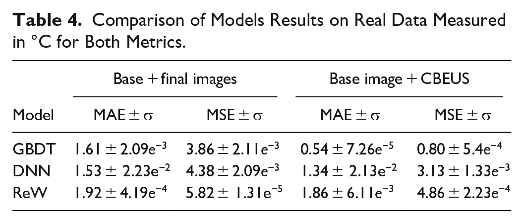
Table 4 shows the results for the porcine muscle. The same characteristics of the previous experiments are presented, with the GBDT model achieving the best results.

Table 4.

Comparison of Models Results on Real Data Measured in °C for Both Metrics.

	Base + final images		Base image + CBEUS
Model	MAE ± σ	MSE ± σ	MAE ± σ	MSE ± σ
GBDT	1.61 ± 2.09e⁻³	3.86 ± 2.11e⁻³	0.54 ± 7.26e⁻⁵	0.80 ± 5.4e⁻⁴
DNN	1.53 ± 2.23e⁻²	4.38 ± 2.09e⁻³	1.34 ± 2.13e⁻²	3.13 ± 1.33e⁻³
ReW	1.92 ± 4.19e⁻⁴	5.82 ± 1.31e⁻⁵	1.86 ± 6.11e⁻³	4.86 ± 2.23e⁻⁴

Discussion

Considering the GBDT model could reach results that are within an acceptable range for clinical applications, we will focus our exploratory data analysis on the results of this model. We took the results of a random iteration of the experiments but, as suggested by the considerably low standard deviation of the results, the same patterns can be found in the other experiments. Although further investigation needs to be performed, we have some initial thoughts on why the other two models could not reach better results.

Regarding the DNN model, it is worth mentioning that it was not possible to perform an exhaustive hyperparameter and topology exploration due to infrastructure limitations, and only a few simple combinations that are commonly used for initial evaluation were tested. Although we can cite works like Shwartz-Ziv and Armon41 that demonstrate that tree-based methods usually outperform DNN on tabular data, there are also a group of DNN models based on transformers architecture – like TransformerTab42 – which was designed for application on this type of data and are candidates for future experiments. The RegressionWiSARD model that was applied presents similar behavior as its classification counterpart: while suboptimal prediction performance when compared to other models, it is a light model that can easily be implemented at hardware level. The main objective was to assess the general performance of this model and evaluate the tradeoff. Also, a wider parameter exploration needs to be performed.

Error Analysis on Numeric Data

Even though the temperature variation can be considered a continuous variable, the data used presented discrete values. In this way, it is possible to analyze what was the error for each expected ∆. As previously mentioned, ∆ represents the expected temperature variation for a given input data. When evaluating the models’ performance, we compare this value with the one predicted by the model. The difference between these two values is what we call prediction error. For the data that was not used for training, we have inputs that should be predicted as ∆ = 1 but are predicted as some other value, which may be small or large. The same holds for ∆ = 2, ∆ = 3, and so on. Then, we performed a separation of this data into groups represented by the respective value of ∆ that should be predicted.

A kernel density estimation (KDE) plot was generated for each group to describe how the absolute value of the prediction error on the group was distributed. Besides, we must consider that we have a starting temperature in each ∆. For example, we can consider a variation of 1°C from 36°C to 37°C or from 42°C to 43°C. In this sense, each plot splits the data for each starting temperature in the form of a colored line. Figures 7 and Figure 8 bring together all KDE plots for the simulated data and the in vitro data, respectively.

Figure 7.

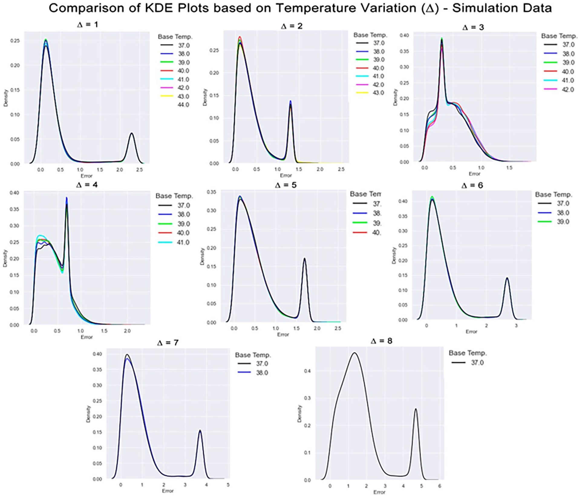
Comparison of KDE plots based on temperature variation on the simulated data. The X-axis indicates the absolute error between the expected output and the predicted value. The Y-axis indicates the number of observations within that range of error indicated by X. In each plot, there is a collection of colored lines that overlap and some points. Each color represents a base temperature. Above each subplot is indicated the temperature variation.

Figure 8.

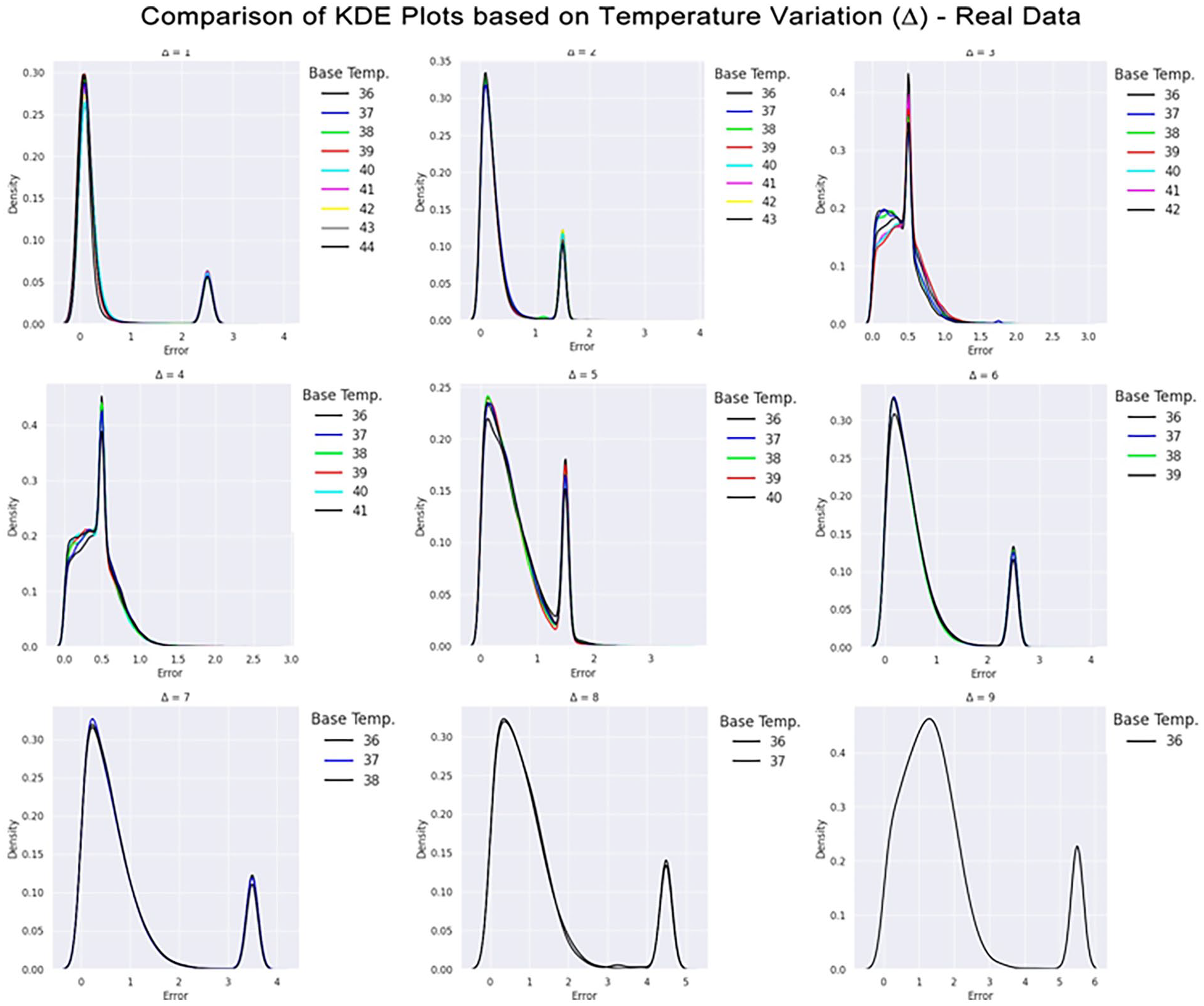
Comparison of KDE plots based on temperature variation on the real data. The X-axis indicates the absolute error between the expected output and the predicted value. The Y-axis indicates the number of observations within that range of error indicated by X. In each plot, there is a collection of colored lines that overlap and some points. Each color represents a base temperature. Above each subplot is indicated the temperature variation.

It is possible to visualize, for example, that there is not a considerable difference in the error distribution between the different starting temperatures, as the lines for all temperatures in the same plot describe similar behavior. This can be related to the monotonic aspect of temperature increase described earlier, and the GBDT model was able to capture it.

A common feature in all plots is the presence of a peak around the value of 3.4°C. This fact was due to the external region composed of water, which always has the same behavior (slope 0). These points appear in all temperature variations and, when combined with the imbalance of classes, cause the result for these points to be given by a weighted average. To better understand this effect, consider a neighborhood k = 1. When considering the external water region, we build inputs by selecting i) pixels in the temperature image with a gray-scale value of 0 (a black pixel) and all 9 pixels within its neighborhood, which are also black in most of the cases), and ii) pixels in the CBEUS image that, in this scenario, presented a slope parameter of 0.0 since there was no variation along the heating procedure. Then, our input would be a zero-array of size 18 (9 from the temperature and 9 from the CBEUS). We encounter this input across all possible temperature variations, which leads to the same input being addressed to all possible expected outputs.

In situations like that, regression models usually output the average value between the possible predictions, which would be 4.5°C in this case. It turns out that the dataset is not balanced: the lower temperature variations appear more than the higher temperature variations. This causes the average to move in the direction of the lower values, and, in our experiments, reach a value around 3.4°C. As this behavior occurs in a significant portion of the dataset, it could create peaks in the KDE plots.

Nevertheless, by considering most of the plots it is possible to observe that prediction errors for smaller ∆ variations are concentrated close to a margin of 0.5°C. On the other hand, as ∆ increases, the prediction error range also increases, although it is worth recalling that there are fewer training observations for high-temperature variation, which can impact the models’ performance. The analysis can also be performed by considering the region where the predictions were made. Figure 9 presents heatmaps obtained from all predictions made for the possible variations considering the base temperature image of 37°C. This temperature image was chosen because it allows all temperature variations in the image set.

Figure 9.

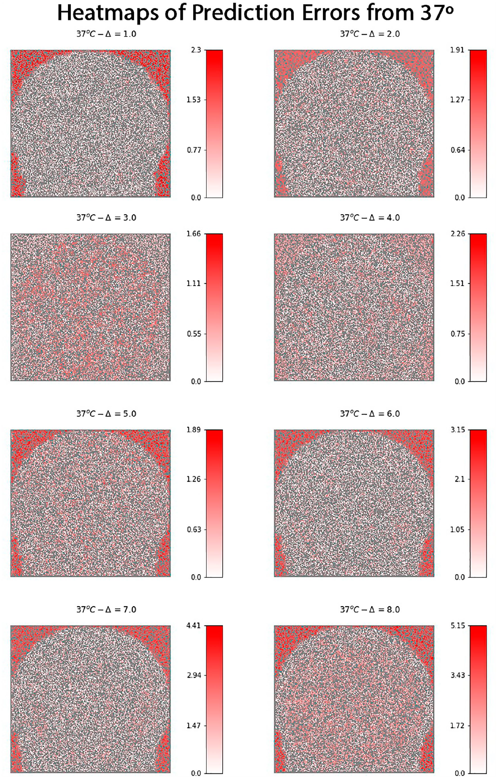
Comparison of prediction error of the GBDT model from a spatial perspective. Each heatmap indicates the absolute value of the error for each classified pixel by coloring it in a gradient that ranges from white to red according to the scale defined next to the graphic. In each heatmap, the gray region indicates pixels that were used for training the model and were not evaluated in the prediction process.

Each heatmap presents a gradient pattern that ranges from white to red. The variable in question is the absolute prediction error, i.e. for each pixel in a given image, the absolute value of the difference between the expected temperature output (represented in the image title) and the prediction made by the model. In each figure, there are two kinds of pixels. Gray pixels were used for training the model or could not be accessed because of neighborhood limitations. All other pixels were used for prediction. Low errors are associated with the white color, as complete white means an error of 0°C. As the error increases, the pixel turns red.

It is possible to observe that, apart from Δ = 3 and Δ = 4, all heatmaps show a concentration of red pixels around the phantom muscle and lipid regions in the phantom, which once again relates to the water medium and the presence of the same variation pattern in all temperatures. The two temperatures that present lower error in these regions are exactly the ones that are close to the weighted average previously mentioned.

Another aspect that is worth mentioning is that the scale of error increases along with the temperature, mainly when considering temperature variations starting from 6°C. One possible explanation is related to imbalanced data, as fewer examples in these groups can affect the prediction performance. On the other hand, once again the region representing the water medium negatively affects the results, since it is concentrated around a value that is closer to the lower temperature variations. Finally, it is important to state that these heatmaps are not supposed to serve practical purposes, but they are of great importance for the data analysis process to demonstrate the model’s performance and reliability, and by giving a spatial perspective of where the model works better.

Error Analysis on Muscle Tissue

As previously observed in the experiments, the prediction performance increased when isolating the analysis within the muscle regions. Figure 10 shows a comparison between the original heatmap generated and a modified version that covers the regions that are not defined as muscle tissue in the phantom. It is possible to observe that red regions cannot be detected clearly, which indicates that the error in this section was small. We could interpret these results as indicating that it would be possible to modify the proposed approach for considering a collection of models that are trained for different tissue types.

Figure 10.

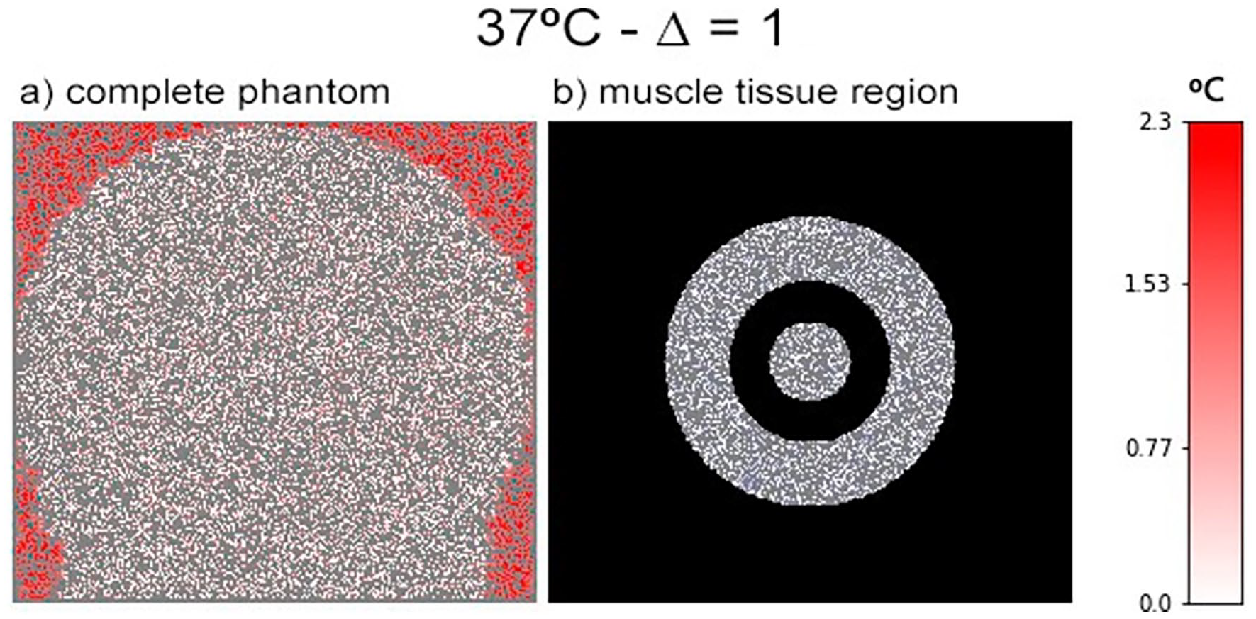
Error visualization of muscle-related region in the phantom figure. (a) the standard heatmap considering the base image at 37°C and temperature variation ∆ = 1, as presented in Figure 9. (b) The same heatmap, but displaying only the regions related to muscle tissue in the phantom.

Conclusion and Future Work

In this work, we sought to present a data-driven model for the problem of estimating the temperature variation in B-mode ultrasound images. The goal was to develop a supervised learning formulation that transformed the ultrasound images into a tabular format and generated a dataset. After the transformation, machine learning algorithms were applied, and measurements were taken to evaluate the models’ performance in predicting the temperature variation. This transformation included the usage of information retrieved from a parametric image generated by analyzing changes in backscattered energy (CBE). The proposed modeling using the CBEUS image encapsulates a novel methodology for estimating temperature variation.

Experiments showed that the gradient-boosted decision tree model (GBDT) could estimate the variation with a mean absolute error of 0.55°C in a simulated environment and 0.41°C when considering only muscle tissue regions. When applying the method to the in vitro real sample, the model presented 0.54°C of mean absolute error. It is worth noticing that errors close to 0.5°C are acceptable in practical environments, both in physiotherapy treatments and high-intensity focused ultrasound (HIFU).

The obtained results point towards a handful of directions for further exploration. As previously mentioned, experimenting a wider range of the used models’ hyperparameters, and applying other methods for performance comparison are the first steps regarding the machine learning aspects of this work. Also, it is worth mentioning that, although the weightless-based model performed worse compared to the other models, the benefits provided by its low power consumption should be stated. Besides that, there are still different parameter configurations and improvements in the binarization techniques that could enhance its overall performance and are also a case of future investigation. Besides that, we also intend to extend the proposed approach in the sense of creating a hybrid model sharing components of other temperature estimation techniques, as well as developing a comparative study of these methods.

Nevertheless, the main objective of this work was the proposal of the data modeling and that it was possible to find a model that could reach the desired results. Although the results provided in this work are highly promising, we consider the current state of this work as a proof of concept, and the clinical application for the presented method still requires more research to be conducted. For example, we did not investigate the method’s performance in a scenario where the temperature changes in terms of position and time, but we can suggest the necessity of combining our approach with a motion-tracking system to capture position changes. We also did not perform specific experiments on scenarios where the temperature does not change uniformly but, considering that the proposed data modeling works at the pixel level, our initial guess is that the method could be applied in this scenario.

Another concern is how the training process could be applied clinically, and this aspect is directly related to data acquisition. The idea is to perform the training process previously with a structured collection of datasets that encapsulates different application scenarios. In fact, we do not expect to create a single model to correctly estimate all kinds of mixing tissues and structures, but individual models specialized at working with specific body regions. Yet, we still expect human interaction to be required for selecting the desired model for the procedure.

Finally, we find it valuable to share early results on our next evaluation steps that demonstrate the time response of the method. Once all the images are acquired, the method can generate the predictions in a small amount of time. For example, the model can generate a 720p resolution image with the predicted values in less than 2 seconds.

Footnotes

Correction (December 2023):

Article updated online to correct affiliation 2. See https://doi.org/10.1177/01617346231225016 for more details.

Declaration of Conflicting Interests

The author(s) declared no potential conflicts of interest concerning the research, authorship, and/or publication of this article.

Funding

The author(s) disclosed receipt of the following financial support for the research, authorship, and/or publication of this article: This research was partially supported by the Brazilian agency National Council for Scientific and Technological Development (CNPq).

ORCID iD

Luiz F. R. Oliveira

References

Brosseau

Yonge

Robinson

Marchand

Judd

Wells

, et al. Thermotherapy for treatment of osteoarthritis. Health Database. 2003;2003:CD004522.

Chan

Perlas

Basics of Ultrasound Imaging. New York, NY: Springer New York; 2011. pp. 13-9.

Training in diagnostic ultrasound: essentials, principles and standards. Report of a WHO Study Group. World Health Organ Tech Rep Ser. 1998;875:i-46; back cover. PMID: 9659004.

Wust

Hildebrandt

Sreenivasa

Rau

Gellermann

Riess

, et al. Hyperthermia in combined treatment of cancer. Lancet Oncology. 2002;3(8):487-97.

Watson

Ultrasound in contemporary physiotherapy practice. Ultrasonics 2008; 48(4): 321–329. The Resurgence of Therapeutic Ultrasound: A 21st Century Phenomenon.

Saccomandi

Schena

Silvestri

Techniques for temperature monitoring during laser-induced thermotherapy: An overview. International journal of hyperthermia: the official journal of European Society for Hyperthermic Oncology, North American Hyperthermia Group 2013; 29.

Lewis

Staruch

Chopra

Thermometry and ablation monitoring with ultrasound. International Journal of Hyperthermia 2015; 31: 1–19.

Simon

VanBaren

Ebbini

Two-dimensional temperature estimation using diagnostic ultrasound. IEEE Transactions on Ultrasonics, Ferroelectrics, and Frequency Control. 1998; 45(4): 1088–1099.

Anand

Kaczkowski

PJ.

Noninvasive measurement of local thermal diffusivity using backscattered ultrasound and focused ultrasound heating. Ultrasound Med Biol. 2008;34(9):1449-64.

10.

Amini

Ebbini

Georgiou

TT.

Noninvasive estimation of tissue temperature via high-resolution spectral analysis techniques. IEEE Trans Biomed Eng. 2005;52:221-8.

11.

Wyatt

Soher

Maccarini

Charles

Stauffer

Macfall

Hyperthermia MRI temperature measurement: evaluation of measurement stabilisation strategies for extremity and breast tumours. Int J Hyperthermia. 2009;25(6):422-33.

12.

Ferreira

Ruano

Intelligent non-invasive modeling of ultrasound- induced temperature in tissue phantoms. Biomedical Signal Processing and Control 2017; 33: 141–150.

13.

Alvarenga

Wilkens

Georg

, et al. Non-invasive estimation of temperature during physiotherapeutic ultrasound application using the average gray-level content of b-mode images: A metrological approach. Ultrasound in Medicine Biology 2017; 43(9): 1938– 1952.

14.

Straube

Arthur

RM.

Theoretical estimation of the temperature dependence of backscattered ultrasonic power for noninvasive thermometry. Ultrasound Med Biol. 1994;20(9): 915-22.

15.

Arthur

Trobaugh

Straube

Moros

EG.

Temperature dependence of ultrasonic backscattered energy in motion-compensated images. IEEE Trans Ultrason Ferroelectr Freq Control. 2005;52:1644-52.

16.

Shaswary

Assi

Yang

, et al. Noninvasive calibrated tissue temperature estimation using backscattered energy of acoustic harmonics. Ultrasonics 2021; 114: 106406.

17.

Rajkomar

Dean

Kohane

Machine learning in medicine. New England Joural of Medicine. 2019;380(14):1347-58.

18.

Giger

ML.

Machine learning in medical imaging. Journal of the American College Radiology. 2018;15(3 Pt B):512-20.

19.

Liu

Wang

Yang

Lei

Liu

, et al. Deep learning in medical ultrasound analysis: A review. Engineering. 2019;5(2):261-75.

20.

Maraci

Bridge

Napolitano

Papageorghiou

Noble

JA.

A framework for analysis of linear ultrasound videos to detect fetal presentation and heartbeat. Medical Image Analysis. 2017;37:22-36.

21.

Zhang

Xiao

Zheng

Wang

Luo

Ultrasound image reconstruction from plane wave radio-frequency data by self-supervised deep neural network. Medical Image Analysis. 2021;70:102018.

22.

Treeby

Cox

. K-wave: matlab toolbox for the simulation and reconstruction of photoacoustic wave fields. J Biomed Opt. 2010;15:021314.

23.

Rigueira

Pastrana-Chalco

Teixeira

, et al. Evaluation of the gray scale intensityvariation of ultrasonic images from porcine muscle tissue as a function of temperature. In 2019 Global Medical Engineering Physics Exchanges/ Pan American Health Care Exchanges (GMEPE/PAHCE). pp. 1–4.

24.

Teixeira

Pastrana-Chalco

Simões

Pedrosa

von Krüger

Alvarenga

, et al. On the feasibility of ultrasound imaging enrichment by medium-temperature changes. Ultrasonic Imaging. 2019;41(1):17-34.

25.

Rokach

Maimon

Decision Trees, volume 6. 2005. pp. 165–192.

26.

Chow

Chen

, et al. Stochastic gradient boosted distributed decision trees. In Proceedings of the 18th ACM conference on Information and knowledge management. pp. 2061–2064.

27.

Schapire

RE.

The strength of weak learnability. Machine Learning. 1990; 5(2): 197-227.

28.

Chen

Guestrin

Xgboost: A scalable tree boosting system. In Proceedings of the 22nd ACM SIGKDD International Conference on Knowledge Discovery and Data Mining, KDD’16. pp. 785-794.

29.

Hijazi

Kumar

Rowen

, et al. Using Convolutional Neural Networks for Image Recognition. San Jose, CA: Cadence Design Systems Inc; 2015. p.9.

30.

Ling

Kang

Zen

Senior

Schuster

Qian

, et al. Deep learning for acoustic modeling in parametric speech generation: A systematic review of existing techniques and future trends. IEEE Signal Processing Magazine. 2015;32(3):35-52.

31.

Abdel-Hamid

Mohamed

Jiang

Deng

Penn

Convolutional neural networks for speech recognition. IEEE Trans Audio Speech Lang Process. 2014;22(10):1533-45.

32.

Bishop

CM.

Neural networks and their applications. Review of Scientific Instruments. 1994;65(6):1803-32.

33.

Ioffe

Szegedy

Batch normalization: Accelerating deep network training by reducing internal covariate shift. CoRR 2015; abs/1502.03167. URL http://arxiv.org/abs/1502.03167.1502.03167.

34.

Hinton

Srivastava

Krizhevsky

Sutskever

Salakhutdinov

(2012) Improving neural networks by preventing co-adaptation of feature detectors. arXiv preprint arXiv:1207.0580

35.

Bledsoe

Browning

Pattern recognition and reading by machine. In: Eastern Joint IRE-AIEE-ACM Computer Conference. New York, NY, USA, pp.225-232.

36.

Aleksander

Thomas

Bowden

PA.

WISARD a radical step forward in image recognition. Sensor Review.1984;4(3):120-4.

37.

Miranda

Arora

Susskind

, et al. Logicwisard: Memoryless synthesis of weightless neural networks. In: 2022 IEEE 33rd International Conference on Application-specific Systems, Architectures and Processors (ASAP). pp.19-26.

38.

Susskind

Arora

Miranda

IDDS

, et al. Weightless neural networks for efficient edge inference, 2022, https://arxiv.org/abs/2203.01479.

39.

Lusquino Filho

LAD

Oliveira

LFR

Lima Filho

, et al. Prediction of palm oil production with an enhanced n-tuple regression network. In: Proceedings of the 27th European Symposium on Artificial Neural Networks, Computational Intelligence and Machine Learning. pp.301-306.

40.

Pedregosa

Varoquaux

Gramfort

, et al. Scikit-learn: Machine learning in Python. Journal of Machine Learning Research. 2011;12:2825-30.

41.

Shwartz-Ziv

Armon

Tabular data: Deep learning is not all you need. CoRR 2021; abs/2106.03253. URL https://arxiv.org/abs/2106.03253.2106.03253.

42.

Huang

Khetan

Cvitkovic

, et al. Tabtransformer: Tabular data modeling using contextual embeddings. CoRR 2020; abs/2012.06678. URL https://arxiv.org/abs/2012.06678.2012.06678.

A Data-Driven Approach for Estimating Temperature Variations Based on B-mode Ultrasound Images and Changes in Backscattered Energy