
Abstract
We revisit the predictive ability of dividend changes for firms’ future earnings and extend the literature by examining the effect of management forecasting ability. Although prior studies have examined the relationship between dividend changes and future earnings, the empirical evidence is mixed. The belief that dividend changes have implications for future earnings depends on the assumption that managers can accurately assess future earnings prospects. In this regard, we posit that the predictive ability of dividends can vary with managers’ forecasting ability. Analyzing a large sample of Japanese dividend-paying firms, we find that dividend changes, particularly dividend increases, are positively associated with increases in future earnings. Consistent with our hypothesis, this positive association is more pronounced for firms with high-forecasting ability managers. Our findings support the signaling theory of dividend changes and indicate that management forecasting ability has a moderating effect on the linkage between firms’ dividend changes and future earnings.
Keywords
Introduction
Previous studies have explored whether dividend changes convey information about future earnings. Miller and Modigliani’s (1961) dividend displacement proposition predicts that, in perfect markets, dividend payments systematically reduce a firm’s market value of equity by the same amount, implying a negative impact on future earnings (Das et al., 2020; Goncharov & Veenman, 2014; Penman & Sougiannis, 1997). Meanwhile, in less-than-perfect markets, managers can use dividends to signal their private information about their firm’s future performance (Ham et al., 2020; Lintner, 1956; Miller & Modigliani, 1961). Lintner (1956) and Brav et al. (2005) document that managers prefer stable dividends and increase them only when they believe their earnings will persistently and sustainably increase, suggesting that dividend changes are positively associated with future earnings. Consistent with these two opposing implications for future earnings, the empirical evidence on the linkage between dividend changes and future earnings has been mixed at best.
In this study, we extend the literature by examining whether the predictive ability of dividends for future earnings varies with managers’ forecasting ability. Specifically, we propose that firms’ dividend changes have a positive association with future earnings, mainly when managers are good at assessing future earnings. One possible reason for the inconsistent findings in prior studies stems from the underlying assumption that managers have perfect information about future earnings (Lintner, 1956; Miller & Modigliani, 1961). However, it is more realistic to assume that uncertainty regarding future earnings and forecasting ability can differ by managers and firms (Baik et al., 2011; Demerjian et al., 2013; Goodman et al., 2014; Ishida et al., 2021). Thus, we posit that managers’ ability to assess future prospects will influence the predictive ability of dividend payouts.
We investigate the predictive ability of dividend changes and their relationship with management forecasting ability using Japanese data. First, Japan is particularly unique for its large number of dividend-paying firms. More than 80% of Japanese listed firms periodically pay cash dividends (Nakano & Takasu, 2012). The prevalence of dividends alleviates the potential self-selection bias of dividend payers and highlights the importance of dividend payments as a signal to differentiate a company from its competitors (Bhattacharya, 1979). Second, Japanese firms generally prefer stable dividends and are reluctant to frequently make changes to their dividend payments (Hanaeda & Serita, 2008). This suggests real costs for changing dividends and enhances the credibility of dividend changes, particularly dividend reductions as signaling mechanisms. Third, firms in the United States can choose dividends or stock repurchases as substitute policies for paying out cash to investors, potentially making dividends less informative in the U.S. context. In contrast, stock repurchases are less common in Japan because Japanese firms attach more importance to dividends as a tool to signal managers’ prospects and do not consider stock repurchases as a substitute (Hanaeda & Serita, 2008). In summary, the Japanese setting has some unique characteristics that make it an excellent setting to test the predictive ability of dividend payouts.
In addition, the Japanese financial disclosure system effectively mandates listed firms to disclose annual management earnings forecasts (Ishida et al., 2021; Kato et al., 2009). Prior studies have used management forecast accuracy as a reasonable proxy for managers’ ability to collect high-quality information and anticipate future changes in the business environment of their firms (Goodman et al., 2014; Lee et al., 2012). Consequently, the institutional arrangements underlying dividends and management earnings forecasts in Japan mitigate potential endogeneity issues concerning both dividends and management forecasts. This study generates a comprehensive sample to test the impact of managers’ forecasting ability on the information conveyed by dividend changes.
Using a sample of 32,570 firm-years of Japanese listed dividend payers for 2002–2018, we examine whether dividend changes convey information about firms’ future profitability and whether the relationship between dividend changes and future earnings varies with managerial forecasting ability. We use the average annual management earnings forecast accuracy for the past 3 years as a proxy for managerial forecasting ability. Applying Fama and MacBeth’s (1973) by-year regression approach, we find that dividend changes, particularly dividend increases, are significantly and positively associated with firms’ profitability in the following year, supporting the dividend signaling theory rather than the dividend displacement proposition. We also find that managerial forecasting ability has a moderating effect on the relationship between dividend changes and future earnings. Specifically, dividend changes made by managers with high-forecasting ability are more likely to be positively associated with firms’ future earnings. These results are robust to many sensitivity tests, including regressions using subsamples partitioned by managerial forecasting ability levels, Theil-Sen regressions, and alternative measurements of managers’ forecasting ability. Overall, our results support the signaling theory of dividends and indicate that the positive relationship between dividend changes and future earnings is more pronounced for firms with high-forecasting ability managers.
We contribute to the literature in several important ways. First, while prior studies document mixed results on the informativeness of dividend changes regarding firms’ future earnings, we provide consistent evidence confirming the favorable implication of dividend increases for Japanese companies. Second, although Jiraporn et al. (2016) examine the relationship between managerial ability and dividend payouts, we provide more direct evidence by focusing on managerial forecasting ability as the driver for the predictive ability of firms’ dividend changes. Third, we extend the literature on management forecast quality. Researchers have examined the effect of managers’ forecasting quality in various other contexts (Goodman et al., 2014; Lee et al., 2012). We link it with the predictive ability of dividend changes, where the relationship is highly plausible. This finding should also be of interest to investors and other capital market participants as it leads to a better assessment of the implications of dividend changes.
The remainder of this paper is organized as follows. The second section provides an institutional background and develops a hypothesis based on related literature. The third section describes the measurement of variables and research design for testing our hypothesis. The fourth section outlines our sample selection procedure and presents the descriptive statistics for variables used in this study. The fifth section discusses the regression results and conducts robustness tests for obtained findings. The final section concludes with a summary.
Institutional Background and Hypothesis Development
Dividend Practices in Japan
There are many dividend-paying firms in Japan, and the vast majority of Japanese listed firms periodically pay cash dividends (Nakano & Takasu, 2012). Figure 1 presents the proportions of firms that pay dividends, conduct stock repurchases, or both by year in Japan. The ratio of dividend payers is approximately 80% of all listed companies throughout the sample period, and more than 50% of Japanese firms pay only dividends. When we focus on the year 2010 after the world financial crisis, the fraction of firms with dividend payments and stock repurchases sharply decline while the number of dividend-only firms rapidly increases. This suggests managers’ strong preference to pay dividends in the Japanese economy, which is in stark contrast to the United States, where stock repurchases are prevalent as a payout to shareholders (Skinner, 2008). 1
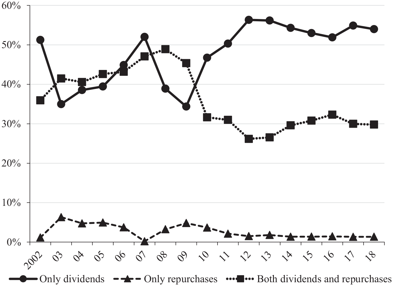
Comparison of dividends and stock repurchases in Japanese firms.
Dividend payment practices in Japan are consistent with the framework of Lintner (1956). Lintner (1956) finds that managers prefer stable dividends and increase them only when managers confidently believe that their earnings will sustainably increase, building a theoretical background for the signaling theory of dividends. Although Lintner’s framework is becoming outdated in the United States (Brav et al., 2005; Skinner, 2008), Sasaki and Hanaeda (2010) document that dividend practices of Japanese firms are highly consistent with the framework. Japanese managers generally prefer stable dividend payouts and determine their dividend practices based on permanent changes in accounting earnings and past dividend levels.
Figure 2 shows dividend payouts among Japanese listed firms by groups based on firms’ annual changes in dividends per share (DPS): Increase, Initiate, Stable, Decrease, Stop, and Nothing. Approximately 35% of firms had stable dividend payouts throughout the sample period. This is true even during the world financial crisis in 2008–2009, suggesting that keeping DPS as a baseline for Japanese dividend practices and temporal shocks provides limited effects on firms’ dividend payouts. Similarly, the world financial crisis caused a Decrease rather than a Stop in DPS in 2008–2009. Meanwhile, the fraction of Increase gradually rises following Abenomics after 2012. 2
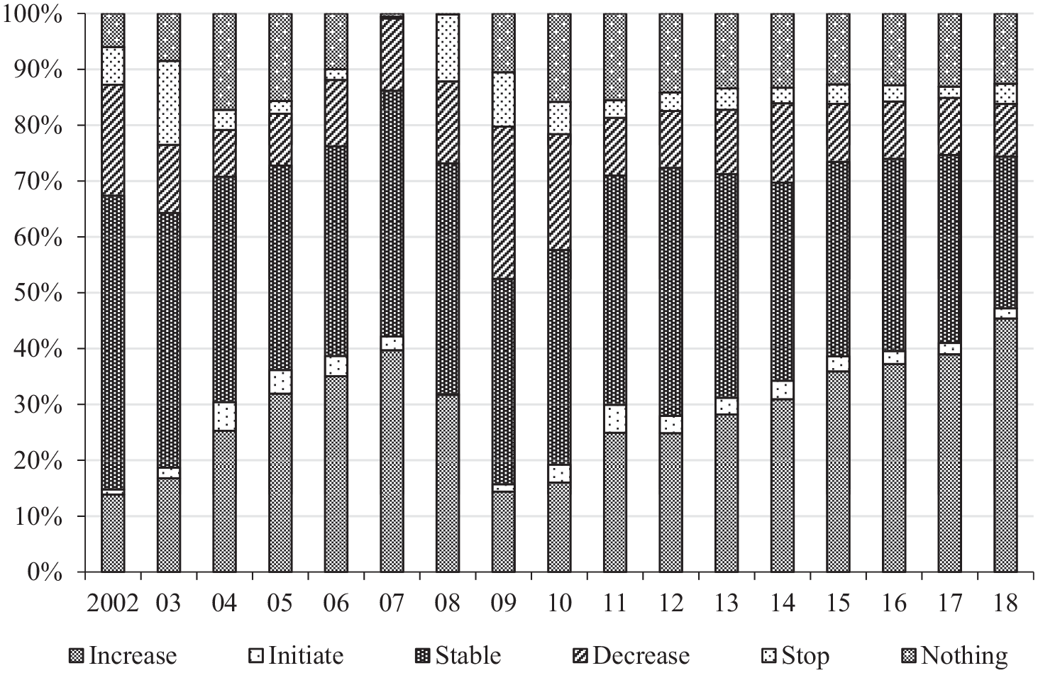
Dividend practices of Japanese firms.
Moreover, regarding the timing of dividend payments, most companies tend to pay dividends once at the fiscal year-end or twice, typically one at the end of the second quarter and the other at the fiscal year-end. Approximately 51.2% of our sample firms pay dividends once at the fiscal year-end, while the remaining 48.4% pay dividends twice at the second quarter and fiscal year-end. 3 Notably, about 60.8% of those firms paying twice paid the same interim dividends as the year-end dividends, indicating that they divide the firms’ annual dividends into halves. These indicate that most Japanese managers tend to determine dividend changes based on the fiscal year.
These characteristics of Japanese dividend practices are useful to examine the predictive ability of firms’ dividend changes. The prevalence of dividends alleviates the potential self-selection bias of dividend payers and highlights the importance of dividends as a signal to differentiate a company from its competitors (Bhattacharya, 1979). Dividends can be a reliable signal for future performance due to their costs. Thus, managers who want to signify their confidence have incentives to utilize dividends as an information channel to capital markets. Moreover, Japanese firms’ dividend changes represent managers’ confidence about future earnings and better reflect their perceptions on earnings prospects. Hanaeda and Serita (2008) replicate Brav et al.’s (2005) survey in a sample of Japanese listed firms. They show that 58% of Japanese managers agree or strongly agree that increases in dividends convey private information about increases in their firms’ future performance. In contrast, only 12% disagree or strongly disagree with the notion.
Hypothesis Development
For the linkage between dividend changes and future earnings, the theory of corporate finance has proposed two opposite predictions. On one hand, the dividend displacement proposition suggests that, in perfect markets, dividends should reduce a firm’s market value of equity by the same amount (Miller & Modigliani, 1961). From the residual income valuation model, this property predicts that dividends systematically reduce future earnings by the expected rate of return on invested capital (Das et al., 2020; Goncharov & Veenman, 2014; Penman & Sougiannis, 1997). On the other hand, in less-than-perfect markets, managers can use dividends to signal their private information or confidence about their firms’ future performance (Lintner, 1956; Miller & Modigliani, 1961). As noted earlier, Lintner (1956) and Brav et al. (2005) argue that managers prefer stable dividends and increase them only when they believe their earnings will persistently and sustainably increase. In such cases, firms’ dividend changes can positively relate to future earnings.
The extant empirical literature provides inconclusive evidence on this linkage. For instance, Penman and Sougiannis (1997) and Fukuda (2000) find that dividends are negatively associated with future earnings, supporting the dividend displacement property. Using the signaling theory, Watts (1973) finds an insignificant relationship between dividend changes and future earnings. Similarly, Benartzi et al. (1997), Grullon et al. (2002), and Grullon et al. (2005) find no positive association between dividend increases and future earnings changes. By contrast, other studies report positive associations between dividend changes and future earnings. Healy and Palepu (1988) investigate dividend initiations and omissions and find that these are positively related to past and future earnings changes. Aharony and Dotan (1994), Nissim and Ziv (2001), Kato et al. (2002), and Ham et al. (2020) find that dividend changes are positively associated with earnings in the following years.
In this study, we extend the literature by examining whether the predictive ability of firms’ dividend changes varies with managers’ forecasting ability. Specifically, we propose that dividend changes have a positive association with future earnings, mainly when managers are good at predicting their firms’ future earnings. One possible reason for the inconsistent evidence stems from the underlying assumption that managers have perfect information about future earnings. Namely, managers are better informed about future earnings and increase/decrease dividends based on their prospects for future earnings (Brav et al., 2005; Lintner, 1956). However, it is challenging for inside managers to predict future earnings accurately (Jensen, 1993). DeAngelo et al. (1996) report that dividends are less likely to be a reliable signal because of managers’ overoptimism. Similarly, Fukuda (2000) finds that dividend changes are negatively associated with subsequent earnings and points out that managers tend to be overly optimistic or pessimistic about future earnings when changing the firm’s dividend payouts.
In light of the above argument, we predict that firms’ dividend changes conveying information about future earnings depend on the managers’ ability to predict future earnings. To the extent that managers differ in their forecasting ability and use dividends to signal their private information or confidence about future performance, we expect that dividend changes are positively associated with future earnings, particularly for firms with high-forecasting ability managers. This leads to our testing hypothesis as follows:
The hypothesis has an underlying assumption: Managers use dividends as a signal for future firm performance. As noted previously, dividend practice in Japanese markets is mainly consistent with Lintner’s (1956) framework, and thus managers tend to utilize dividends as a signal for their confidence about future performance (Hanaeda & Serita, 2008; Sasaki & Hanaeda, 2010). However, given that there are two competing predictions on the relation between dividend changes and future earnings (i.e., dividend displacement proposition and signaling theory), the relationship itself can be either positive or negative and thus an empirical issue. Accordingly, we first examine the relationship between dividend changes and future performance as a preliminary test. In the presence of dividend displacement property (i.e., a negative association between dividend changes and future earnings), our hypothesis predicts that the effect of managers’ forecasting ability can reduce the size of the negative association (or make it positive). Meanwhile, in the presence of a signaling effect (i.e., a positive association between dividend changes and future earnings), we expect the positive association to be more pronounced for firms with managers of higher forecasting ability.
Research Design
Proxy for Managers’ Forecasting Ability
To measure managers’ forecasting ability, we follow Goodman et al.’s (2014) method and use the accuracy of management earnings forecasts. We define managerial forecasting ability as managers’ competence to collect high-quality information regarding internal operations and the external environment and process and synthesize this information to develop accurate forecasts about the firm’s future performance. Management forecast accuracy can be a proxy for managers’ forecasting ability as it can represent their ability to gather and process relevant information to make accurate forecasts (Goodman et al., 2014).
The Japanese financial disclosure system helps examine management forecasting ability because it effectively requires managers to issue earnings forecasts. As recommended by the Tokyo Stock Exchange, Japanese listed firms are obligated to release 1-year ahead point estimates within 45 days of the fiscal year-end (Kato et al., 2009; Ishida et al., 2021). About 94.6% of our initial sample firms issued annual management earnings forecasts at the beginning of the fiscal year. Thus, unlike in the United States, where management earnings forecasts are voluntary, the Japanese setting yields unbiased observations of management earnings forecasts. Moreover, management forecast accuracy can be a reasonable proxy for managers’ forecasting ability in Japan. Japanese managers generally have an incentive to issue accurate initial forecasts due to the negative consequences of issuing inaccurate forecasts (Ishida et al., 2021; Otomasa et al., 2020).
We measure management forecasting ability, MFA, using the average forecast accuracy for annual earnings forecasts in the past 3 years (years t− 2 to t) multiplied by −1. Forecast accuracy is defined as the absolute value of the differences between the forecasted net income issued at the beginning of the fiscal year and the actual reported net income, scaled by the lagged market value of equity. Thus, MFA takes a higher value for firms/managers with higher forecasting ability. The long measurement window helps mitigate short-term effects that may bias forecast accuracy, such as earnings management or short periods of forecasting “luck” (Goodman et al., 2014).
Regression Models
We test our hypothesis by applying regression models introduced by Nissim and Ziv (2001). 4 We estimate the following two models for the predictive ability of firms’ dividend changes about future changes and levels in earnings, respectively:

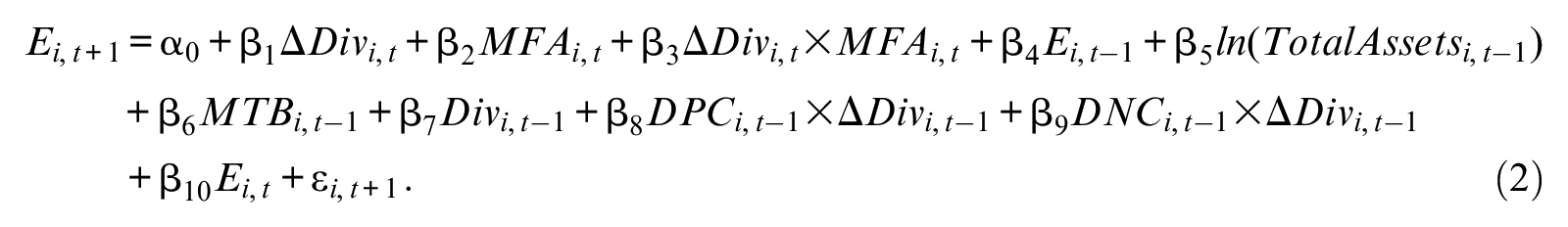
where ΔEi,t+1 is the annual change in earnings measured as net income before extraordinary items from year t to year t+ 1, and Ei,t+1 is earnings measured as net income before extraordinary items in year t+ 1. Both are deflated by the book value of equity at the end of year t− 1 (Grullon et al., 2005; Nissim & Ziv, 2001). Equation 1 represents the estimation model for changes in earnings, and Equation 2 is for the level of earnings in the following year of cash dividend payouts.
For the independent variables, ΔDivi, t denotes the rate of annual changes in DPS from years t− 1 to t (Grullon et al., 2005; Nissim & Ziv, 2001). Ham et al. (2020) use quarterly data and an event window approach that compares earnings announced after the dividend change to earnings before the dividend change. However, as noted earlier, most Japanese firms determine dividend changes based on the fiscal year and rarely pay quarterly dividends. Thus, we use the fiscal year approach to measure dividend changes and compare earnings based on the fiscal year. 5
Our variable of interest is the interaction term (ΔDivi, t ×MFAi, t ), and its coefficient β3 indicates the moderating effect of managerial forecasting ability on the predictive ability of dividend changes. Based on our hypothesis, we expect coefficient β3 to be significantly positive for both Equations 1 and 2.
In addition, we extend the estimation models by including indicator variables for dividend changes to allow different coefficients on dividend increases and decreases. Nissim and Ziv (2001) point out that the predictive ability can differ between dividend increases and decreases. Accordingly, we also specify the following modified models for estimation:
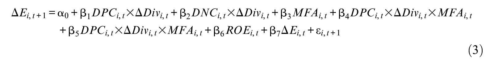
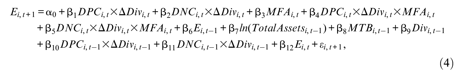
where DPCi,t (DNCi, t ) is an indicator variable equal to one for dividend increases (decreases) and zero otherwise. In Equations 3 and 4, β1 and β2 reflect the predictive ability of dividend increases and decreases, respectively. To test our hypothesis, we focus on the triple interaction terms (DPCi, t ×ΔDivi, t ×MFAi, t and DNCi, t ×ΔDivi, t ×MFAi, t ). If dividend changes made by high-forecasting ability managers have a more positive association with future earnings, we predict coefficients β4 and β5 to be significantly positive. Other independent variables are based on Nissim and Ziv’s (2001) method and control for earnings patterns and mean reversion of accounting earnings. Appendix A provides variable definitions.
To account for heteroskedasticity and autocorrelation in the regression residuals, we use Fama and MacBeth’s (1973) procedure to estimate the coefficients of the regression models (Grullon et al., 2005; Nissim & Ziv, 2001). We estimate cross-sectional regression coefficients each year using all the observations in that year. We then compute the time-series means of the cross-sectional coefficients and apply Hansen and Hodrick’s (1980) standard error correction method to estimate the standard deviations for the means. 6
Sample Selection and Descriptive Statistics
Our initial sample consists of 68,490 firm-year observations of all Japanese listed firms for 2002–2018. The sample period begins from 2002 as we require management forecast data for the preceding 3 years to construct MFA. 7 Our sample period ended in 2018, and we use data in year t+ 1 as future performance. We collect all financial, stock price, and management forecast data from the Nikkei NEEDS-FinancialQUEST, a comprehensive commercial database for Japanese firms. See Table 1 for a summary of our sample selection procedure.
Sample Selection.
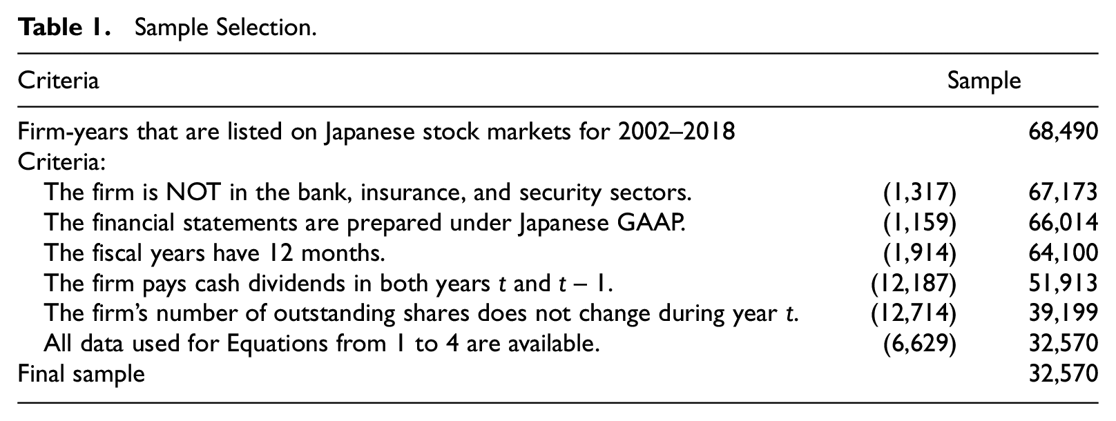
Following prior studies (Grullon et al., 2005; Ham et al., 2020; Nissim & Ziv, 2001), we exclude financial sector firms (i.e., firms in the banking, securities, and insurance sectors) based on the Tokyo Stock Exchange Industry Classification, which classifies all Japanese listed firms into 33 industries. Moreover, we focus on firms that pay dividends in both current and previous years (i.e., years t and t− 1). Similarly, for other distribution events, such as stock splits, stock dividends, and mergers, we exclude firm-years whose number of outstanding shares changes during year t. When firms do not prepare consolidated financial statements, we use unconsolidated accounting data. Thus, the final sample consists of 32,570 firm-year observations.
Table 2 presents the descriptive statistics for variables used in this study. To mitigate the impact of outliers, we winsorize all continuous variables at the top and bottom 1% by year. The table shows that the first quartile and median of ΔDivi, t take values of zero. This is consistent with Figure 2 and suggests that there are a large number of firms that do not change their dividend practices. The mean values of DPCi, t and DNCi, t indicate that approximately 34.4% and 10.4% of the sample firms increase and decrease dividends, respectively, while the remaining 55.2% keep their DPS constant. The distribution indicates “downward stickiness” of dividends and suggests that Japanese firms tend to be more reluctant to decrease dividends than increase them (Hanaeda & Serita, 2008).
Descriptive Statistics.
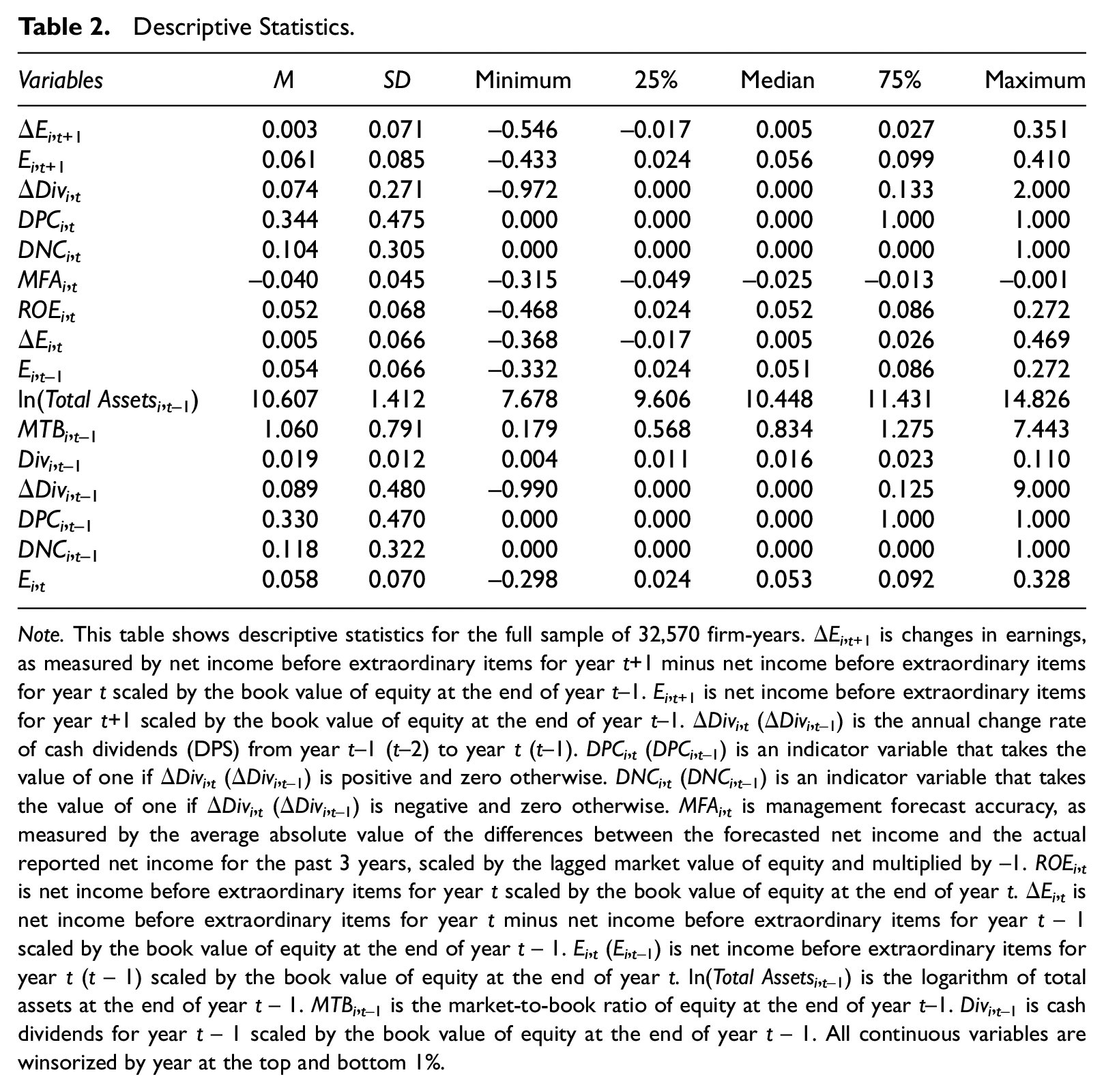
Note. This table shows descriptive statistics for the full sample of 32,570 firm-years. ΔEi,t+1 is changes in earnings, as measured by net income before extraordinary items for year t+1 minus net income before extraordinary items for year t scaled by the book value of equity at the end of year t−1. Ei,t+1 is net income before extraordinary items for year t+1 scaled by the book value of equity at the end of year t−1. ΔDivi, t (ΔDivi,t−1) is the annual change rate of cash dividends (DPS) from year t−1 (t−2) to year t (t−1). DPCi, t (DPCi,t−1) is an indicator variable that takes the value of one if ΔDivi, t (ΔDivi,t−1) is positive and zero otherwise. DNCi, t (DNCi,t−1) is an indicator variable that takes the value of one if ΔDivi, t (ΔDivi,t−1) is negative and zero otherwise. MFAi, t is management forecast accuracy, as measured by the average absolute value of the differences between the forecasted net income and the actual reported net income for the past 3 years, scaled by the lagged market value of equity and multiplied by −1. ROEi, t is net income before extraordinary items for year t scaled by the book value of equity at the end of year t. ΔEi, t is net income before extraordinary items for year t minus net income before extraordinary items for year t− 1 scaled by the book value of equity at the end of year t− 1. Ei, t (Ei,t−1) is net income before extraordinary items for year t (t− 1) scaled by the book value of equity at the end of year t. ln(Total Assetsi,t−1) is the logarithm of total assets at the end of year t− 1. MTBi,t−1 is the market-to-book ratio of equity at the end of year t−1. Divi,t−1 is cash dividends for year t− 1 scaled by the book value of equity at the end of year t− 1. All continuous variables are winsorized by year at the top and bottom 1%.
Table 3 shows the correlation matrix for testing variables. We find that ΔDivi, t is positively correlated with Ei,t+1 but negatively correlated with ΔEi,t+1. However, given that a firm’s profitability is mean-reverting (Fama & French, 2000), the expected changes in earnings tend to be negatively correlated with dividend changes because dividend changes are positively correlated with current profitability. Consistent with this argument, the Pearson (Spearman) correlation coefficient between ΔDivi, t and ΔEi, t is 0.345 (0.388), suggesting the presence of mean-reverting in the following years. This highlights the need to control for the current earnings change (Nissim & Ziv, 2001). 8
Correlation Matrix.
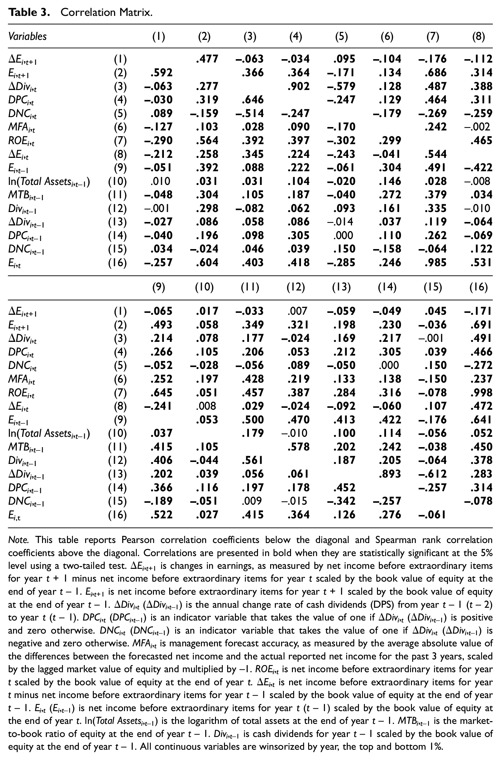
Note. This table reports Pearson correlation coefficients below the diagonal and Spearman rank correlation coefficients above the diagonal. Correlations are presented in bold when they are statistically significant at the 5% level using a two-tailed test. ΔEi,t+1 is changes in earnings, as measured by net income before extraordinary items for year t+ 1 minus net income before extraordinary items for year t scaled by the book value of equity at the end of year t− 1. Ei,t+1 is net income before extraordinary items for year t+ 1 scaled by the book value of equity at the end of year t− 1. ΔDivi, t (ΔDivi,t−1) is the annual change rate of cash dividends (DPS) from year t− 1 (t− 2) to year t (t− 1). DPCi, t (DPCi,t−1) is an indicator variable that takes the value of one if ΔDivi, t (ΔDivi,t−1) is positive and zero otherwise. DNCi, t (DNCi,t−1) is an indicator variable that takes the value of one if ΔDivi, t (ΔDivi,t−1) is negative and zero otherwise. MFAi, t is management forecast accuracy, as measured by the average absolute value of the differences between the forecasted net income and the actual reported net income for the past 3 years, scaled by the lagged market value of equity and multiplied by −1. ROEi, t is net income before extraordinary items for year t scaled by the book value of equity at the end of year t. ΔEi, t is net income before extraordinary items for year t minus net income before extraordinary items for year t− 1 scaled by the book value of equity at the end of year t− 1. Ei, t (Ei,t−1) is net income before extraordinary items for year t (t− 1) scaled by the book value of equity at the end of year t. ln(Total Assetsi,t−1) is the logarithm of total assets at the end of year t− 1. MTBi,t−1 is the market-to-book ratio of equity at the end of year t− 1. Divi,t−1 is cash dividends for year t− 1 scaled by the book value of equity at the end of year t− 1. All continuous variables are winsorized by year, the top and bottom 1%.
Empirical Results and Discussions
Regression Results
Table 4 reports the regression results of Equations 1 and 3, examining the relationship between changes in dividends and changes in future earnings. As mentioned earlier, we apply Fama and MacBeth’s (1973) cross-sectional estimation and report the time-series means of the cross-sectional coefficients and t-statistics based on Hansen and Hodrick’s (1980) standard errors.
Regression Results: Changes in Earnings.
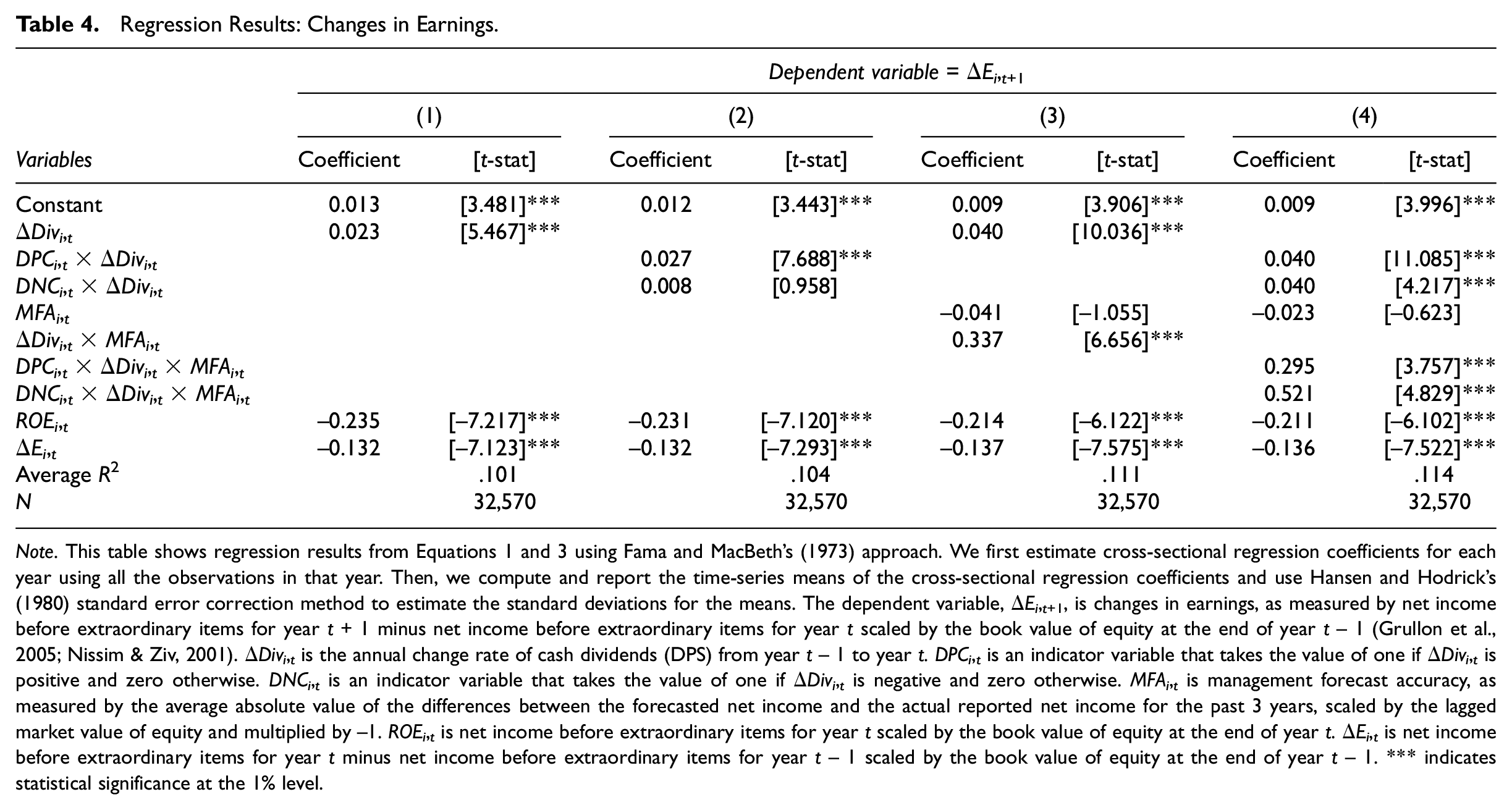
Note. This table shows regression results from Equations 1 and 3 using Fama and MacBeth’s (1973) approach. We first estimate cross-sectional regression coefficients for each year using all the observations in that year. Then, we compute and report the time-series means of the cross-sectional regression coefficients and use Hansen and Hodrick’s (1980) standard error correction method to estimate the standard deviations for the means. The dependent variable, ΔEi,t+1, is changes in earnings, as measured by net income before extraordinary items for year t+ 1 minus net income before extraordinary items for year t scaled by the book value of equity at the end of year t− 1 (Grullon et al., 2005; Nissim & Ziv, 2001). ΔDivi, t is the annual change rate of cash dividends (DPS) from year t− 1 to year t. DPCi, t is an indicator variable that takes the value of one if ΔDivi, t is positive and zero otherwise. DNCi, t is an indicator variable that takes the value of one if ΔDivi, t is negative and zero otherwise. MFAi, t is management forecast accuracy, as measured by the average absolute value of the differences between the forecasted net income and the actual reported net income for the past 3 years, scaled by the lagged market value of equity and multiplied by −1. ROEi, t is net income before extraordinary items for year t scaled by the book value of equity at the end of year t. ΔEi, t is net income before extraordinary items for year t minus net income before extraordinary items for year t− 1 scaled by the book value of equity at the end of year t− 1. *** indicates statistical significance at the 1% level.
Columns (1) and (2) present the results of underlying regressions for testing the predictive ability of dividend changes. As we can observe from Column (1), the coefficient on ΔDivi, t is positive and statistically significant at the 1% level, indicating that dividend changes are likely to associate with future earnings changes positively. Meanwhile, Column (2) shows that only the coefficient on DPCi, t ×ΔDivi, t is positive and significant. Thus, the results suggest that only dividend increases positively relate to future earnings changes. This asymmetric finding is consistent with the descriptive statistics that show Japanese firms are more reluctant to decrease dividends. In this case, dividend decreases are less likely to reflect current changes in managers’ expectations for future earnings, hindering the predictive ability of decreased dividends. 9 These results suggest that in Japan, dividend changes, particularly dividend increases, support the signaling theory rather than the effect of dividend displacement property.
Columns (3) and (4) test our hypothesis for the effect of managerial forecasting ability. As shown in Column (3) using Equation 1, the coefficient on ΔDivi, t ×MFAi, t is 0.337 and significant at the 1% level. Similarly, Column (4) using Equation 3 shows that the triple interaction terms for both dividend increases and decreases (DPCi, t ×ΔDivi, t ×MFAi, t and DPCi, t ×ΔDivi, t ×MFAi, t ) exhibit positive and significant coefficients, suggesting that the predictive ability of dividend changes depends on managers’ forecasting ability. These results support our hypothesis and indicate that dividend changes made by managers with higher forecasting ability are more likely to be positively associated with future earnings.
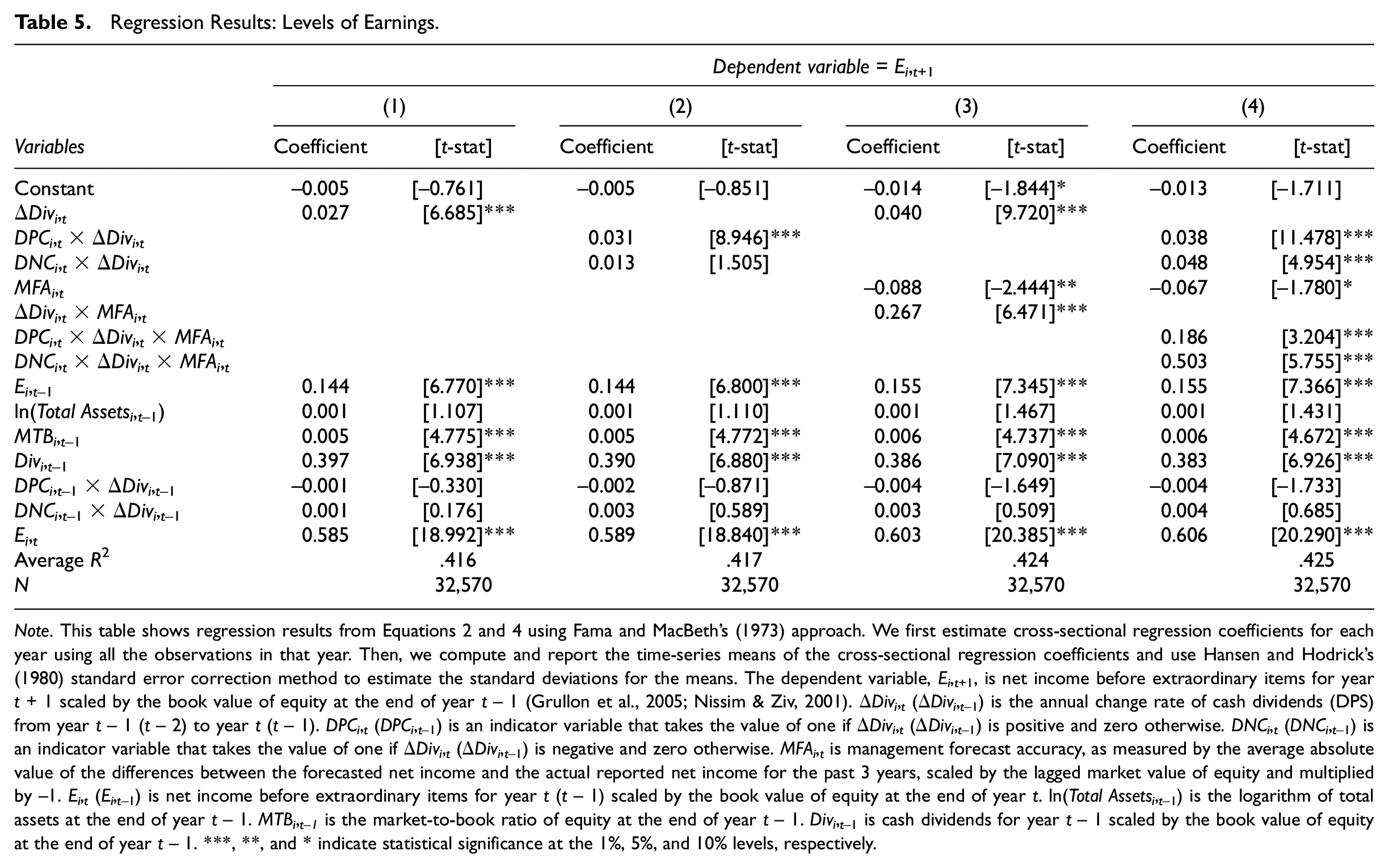
Table 5 presents the regression results of Equations 2 and 4, testing the relation between dividend changes and the level of earnings in the following year. As shown in Columns (1) and (2), dividend changes positively relate to future earnings, and the significant relation is obtained only for dividend increases, which is consistent with that reported in Table 4. Columns (3) and (4) show the effect of managerial forecasting ability. From Column (3) using Equation 2, we again find that the coefficient on ΔDivi, t ×MFAi, t is positive and significant at the 1% level. Moreover, Column (4) using Equation 4 reports that both coefficients on DPCi, t ×ΔDivi, t ×MFAi, t and DNCi, t ×ΔDivi, t ×MFAi, t are positive and significant at the 1% levels. These results are consistent with those in Table 4 and suggest that dividend changes made by high-forecasting ability managers are more predictive of the level of firms’ future earnings.
Regression Results: Levels of Earnings.
Note. This table shows regression results from Equations 2 and 4 using Fama and MacBeth’s (1973) approach. We first estimate cross-sectional regression coefficients for each year using all the observations in that year. Then, we compute and report the time-series means of the cross-sectional regression coefficients and use Hansen and Hodrick’s (1980) standard error correction method to estimate the standard deviations for the means. The dependent variable, Ei,t+1, is net income before extraordinary items for year t+ 1 scaled by the book value of equity at the end of year t− 1 (Grullon et al., 2005; Nissim & Ziv, 2001). ΔDivi, t (ΔDivi,t−1) is the annual change rate of cash dividends (DPS) from year t− 1 (t− 2) to year t (t− 1). DPCi, t (DPCi,t−1) is an indicator variable that takes the value of one if ΔDivi, t (ΔDivi,t−1) is positive and zero otherwise. DNCi, t (DNCi,t−1) is an indicator variable that takes the value of one if ΔDivi, t (ΔDivi,t−1) is negative and zero otherwise. MFAi, t is management forecast accuracy, as measured by the average absolute value of the differences between the forecasted net income and the actual reported net income for the past 3 years, scaled by the lagged market value of equity and multiplied by −1. Ei, t (Ei,t−1) is net income before extraordinary items for year t (t− 1) scaled by the book value of equity at the end of year t. ln(Total Assetsi,t−1) is the logarithm of total assets at the end of year t− 1. MTBi,t−1 is the market-to-book ratio of equity at the end of year t− 1. Divi,t−1 is cash dividends for year t− 1 scaled by the book value of equity at the end of year t− 1. ***, **, and * indicate statistical significance at the 1%, 5%, and 10% levels, respectively.
Overall, our regression analyses suggest that dividend increases have positive implications for both the changes and the levels of future earnings and that managerial forecasting ability provides a moderating effect on the linkage between firms’ dividend changes and future earnings. Thus, consistent with our hypothesis, the predictive ability of dividend changes can be affected by managers’ ability to assess future performance accurately.
Robustness Checks
In this section, we conduct several additional tests to evaluate the robustness of our empirical results.
Regression analysis by MFA group
We partition the sample based on the terciles of MFAi, t by year, and separately run regressions by year for each group. Specifically, we examine how many times the coefficients on ΔDivi, t for the third tercile group (high-MFA firm group) are greater than those for the first tercile group (low-MFA firm group) across sample years and whether the mean values of the coefficients are higher for the high-MFA group than that for the low-MFA group. This alternative approach is helpful because it does not depend on interaction terms of multiple variables and enables us to evaluate how consistent the results are throughout the sample period.
Table 6 shows the results. In the table, the significant proportion indicates the percentage of statistically significant coefficients at the 5% level among 17 years of estimations. In the “3rd vs. 1st tercile groups” column, the positive proportion denotes the percentage of the coefficients of the high-MFA group that are greater than those of the low-MFA group. The t-statistics indicate the statistical significance of the difference in coefficients between the high- and low-MFA firm groups using Welch’s t test. Panels A and B show estimation results for the changes in future earnings and the level of future earnings using the underlying models of Equations 1 and 2, respectively. In Panel A, the coefficients on ΔDivi, t for the high-MFA group are more likely to be more significant than those for the low-MFA group. We observe a significant difference in the mean value of the coefficient at the 5% level.
Robustness Test: Regressions by MFA Group.
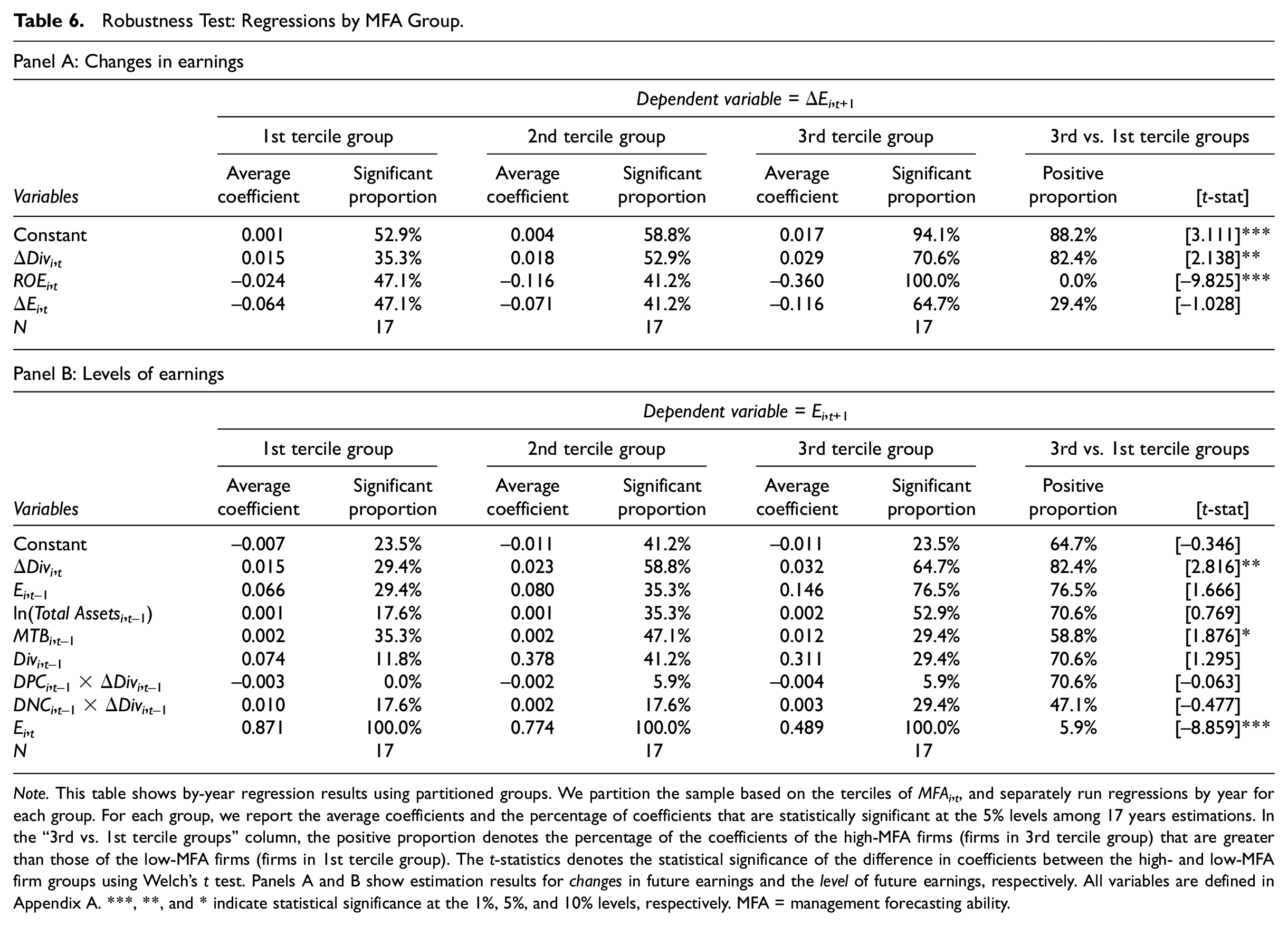
Note. This table shows by-year regression results using partitioned groups. We partition the sample based on the terciles of MFAi, t , and separately run regressions by year for each group. For each group, we report the average coefficients and the percentage of coefficients that are statistically significant at the 5% levels among 17 years estimations. In the “3rd vs. 1st tercile groups” column, the positive proportion denotes the percentage of the coefficients of the high-MFA firms (firms in 3rd tercile group) that are greater than those of the low-MFA firms (firms in 1st tercile group). The t-statistics denotes the statistical significance of the difference in coefficients between the high- and low-MFA firm groups using Welch’s t test. Panels A and B show estimation results for changes in future earnings and the level of future earnings, respectively. All variables are defined in Appendix A. ***, **, and * indicate statistical significance at the 1%, 5%, and 10% levels, respectively. MFA = management forecasting ability.
Similarly, Panel B shows that the coefficients on ΔDivi, t for the high-MFA group are greater than those for the low-MFA group in 14 of 17 by-year estimations (i.e., the positive proportion is 82.4%), and there is a significant difference. For both panels, the average coefficients on ΔDivi, t tend to increase with MFA tercile ranks, indicating that managers’ forecasting ability strengthens the positive association between firms’ dividend changes and future earnings. These results are consistent with our hypothesis.
Alternative scalers for dividend changes and earnings
Following Nissim and Ziv (2001) and Grullon et al. (2005), we scale earnings by the book value of equity and measure dividend changes as the rate of annual changes in DPS from years t− 1 to t. However, previous studies use alternative scalers for earnings and dividend changes, and it may be possible that the choice of scalers affects the empirical results. To assess the sensitivity to alternative scalers, we first use total assets and market capitalization at the end of year t− 1 as scaling variables (Goncharov & Veenman, 2014; Ham et al., 2020). Specifically, we apply these alternative scalers for all earnings variables (i.e., ΔE and E) in equations. Moreover, we use stock price and total assets per share as alternative scalers for ΔDiv. The untabulated results using these alternative scalers are similar to those reported in the primary analysis.
Theil-Sen regressions
We further assess the robustness of our results using the Theil-Sen regression technique, according to Theil (1950) and Sen (1968). The Theil-Sen regression can be a robust alternative method to alleviate the impacts of scaling variables and outliers, as it chooses the median slopes among all lines of groups through n-dimensional sample points, where n is the number of parameters estimated (Das et al., 2020; Ohlson & Kim, 2015).
To conduct the Theil-Sen regression, we modify Equations 1 and 2 and estimate the following two models that use raw and unscaled variables:

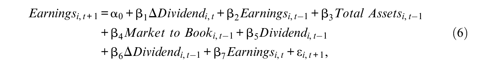
where ΔEarnings is the annual change in net income before extraordinary items from the previous year, and Earnings is earnings measured as net income before extraordinary items in a fiscal year. ΔDividendi, t (ΔDividendi,t−1) is the annual change in dividends from years t− 1 (t− 2) to t (t− 1). Total Assetsi,t−1 is total assets at the end of year t− 1. Market to Booki,t−1 is calculated as market capitalization at the end of year t− 1 minus the book value of equity at the end of year t− 1. Dividendi,t−1 is cash dividends for year t− 1. All variables are unscaled and unwinsorized.
We test our hypothesis with the Theil-Sen regression by following the procedures outlined in Ohlson and Kim (2015) and Das et al. (2020). First, we extract firm observations that increase and decrease their dividends from the previous year and form two groups (i.e., Increase and Decrease firm groups). 10 We then partition each group based on the terciles of management forecast accuracy by year and randomly draw 10,000 subsamples with N observations for each partitioned group, where N is the number of regression parameters estimated. Next, we regress dependent variables on the N− 1 independent variables. Specifically, we run 10,000 such regressions for each of the 17 sample years from 2002 to 2018. For each of these 10,000 regressions, we get N regression parameters (i.e., α0 and the N− 1 β coefficients). Third, within each year, we take the median of each regression parameter from the 10,000 estimated parameters, yielding N regression parameter medians for each year. These N regression parameter medians represent one set of parameter estimates for each sample year.
To test whether the obtained regression parameters are statistically different from zero, we follow Das et al. (2020) and apply a similar approach as Fama and MacBeth (1973). For each of the N parameter estimates in a year, we use the distribution of the 17 annual medians to calculate time-series averages, conduct t tests and determine the statistical significances. As we estimate each regression by year, a given firm can show up once or not at all in a single regression. Therefore, it is not necessary, nor possible, to include year or firm fixed effects in the Theil-Sen regression approach (Das et al., 2020).
Table 7 reports the regression results of Equation 5, examining the relationship between changes in dividends and changes in future earnings. Panels A and B show the results of Increase and Decrease firms, respectively. In both panels, the coefficients on ΔDividendi, t for the third tercile group (high-MFA group) are positive and significant at the 1% levels and likely to be more significant than those for the first tercile group (low-MFA group).
Theil-Sen Regression Approach: Changes in Earnings.
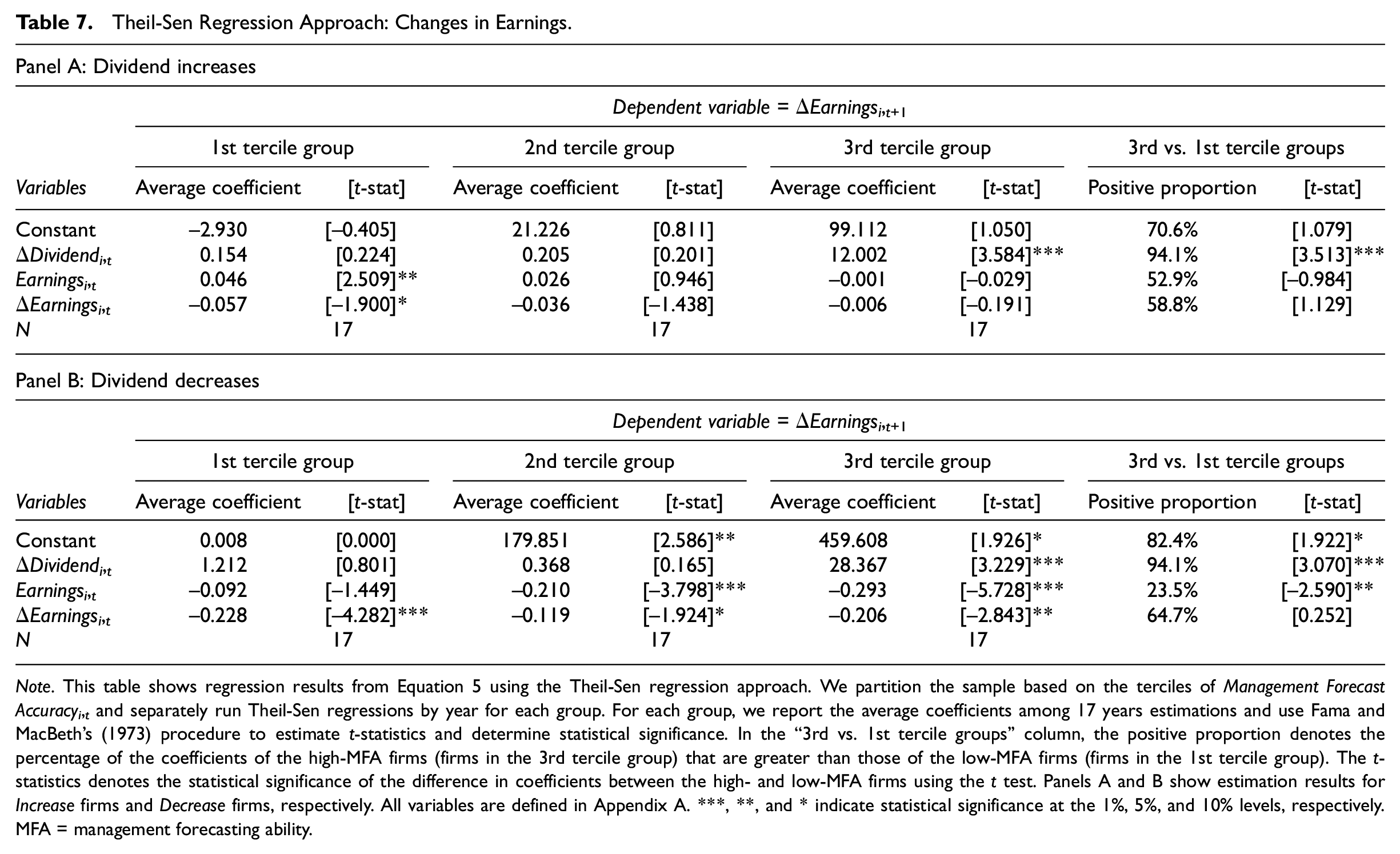
Note. This table shows regression results from Equation 5 using the Theil-Sen regression approach. We partition the sample based on the terciles of Management Forecast Accuracyi, t and separately run Theil-Sen regressions by year for each group. For each group, we report the average coefficients among 17 years estimations and use Fama and MacBeth’s (1973) procedure to estimate t-statistics and determine statistical significance. In the “3rd vs. 1st tercile groups” column, the positive proportion denotes the percentage of the coefficients of the high-MFA firms (firms in the 3rd tercile group) that are greater than those of the low-MFA firms (firms in the 1st tercile group). The t-statistics denotes the statistical significance of the difference in coefficients between the high- and low-MFA firms using the t test. Panels A and B show estimation results for Increase firms and Decrease firms, respectively. All variables are defined in Appendix A. ***, **, and * indicate statistical significance at the 1%, 5%, and 10% levels, respectively. MFA = management forecasting ability.
Table 8 shows the regression results of Equation 6, testing the relation between dividend changes and the level of earnings in the following year. Again, Panels A and B report the results of Increase and Decrease firms, respectively. In Panel A, we find that the coefficients on ΔDividendi, t for the high-MFA group are positive and significant at the 5% levels and more likely to be greater than those for the low-MFA group. Meanwhile, Panel B shows that the coefficients on ΔDividendi, t for the high-MFA group are positive but insignificant, and the difference between the high- and low-MFA groups is not statistically significant. These results are consistent with the main findings, suggesting that our results are robust for the Theil-Sen regression approach. 11
Theil-Sen Regression Approach: Levels of Earnings.
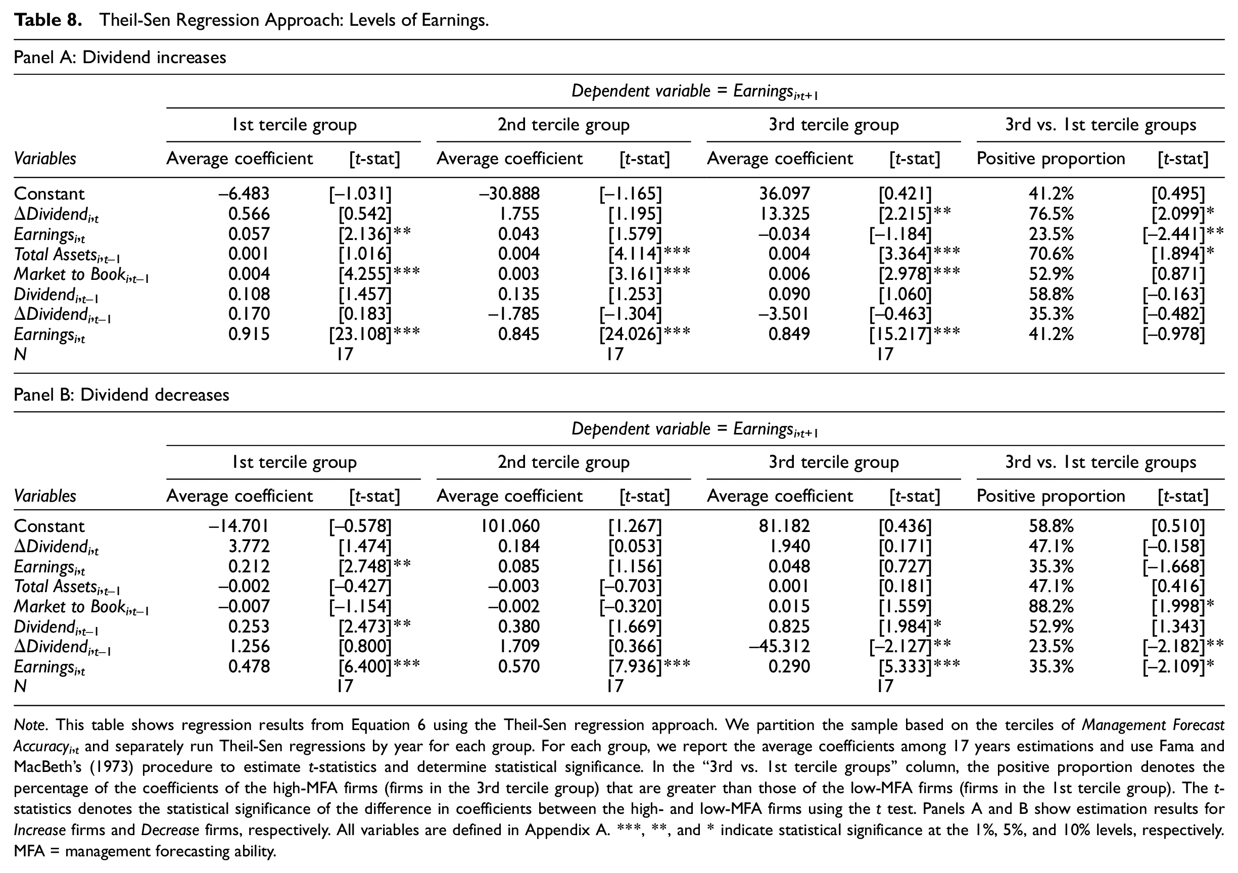
Note. This table shows regression results from Equation 6 using the Theil-Sen regression approach. We partition the sample based on the terciles of Management Forecast Accuracyi, t and separately run Theil-Sen regressions by year for each group. For each group, we report the average coefficients among 17 years estimations and use Fama and MacBeth’s (1973) procedure to estimate t-statistics and determine statistical significance. In the “3rd vs. 1st tercile groups” column, the positive proportion denotes the percentage of the coefficients of the high-MFA firms (firms in the 3rd tercile group) that are greater than those of the low-MFA firms (firms in the 1st tercile group). The t-statistics denotes the statistical significance of the difference in coefficients between the high- and low-MFA firms using the t test. Panels A and B show estimation results for Increase firms and Decrease firms, respectively. All variables are defined in Appendix A. ***, **, and * indicate statistical significance at the 1%, 5%, and 10% levels, respectively. MFA = management forecasting ability.
Alternative measurement for managerial forecasting ability
We assess the robustness of our results using an alternative measure for management forecasting ability. For our primary analysis, we use management forecast accuracy as a proxy for managers’ forecasting ability. However, this measurement may be noisy because the accuracy of management forecasts can be firm-specific, depending on the firm’s characteristics and information environment (Baik et al., 2011; Rogers & Stocken, 2005). It may also be subject to managerial opportunism, such as biased forecasts and earnings management (Ishida et al., 2021; Kato et al., 2009).
Alternatively, we apply the Managerial Ability (MA) Score developed by Demerjian et al. (2012). Demerjian et al. (2013) note that more able managers are more knowledgeable about the firm and the industry and thus better able to synthesize information into reliable forward-looking estimates. Consistently, they report that high-ability managers are associated with higher earnings quality in subsequent periods. Moreover, Baik et al. (2011) and Ishida et al. (2021) examine the accuracy of management earnings forecasts for U.S. and Japanese firms, respectively, and find that high-ability managers tend to issue accurate earnings forecasts. Although the MA Score is essentially an efficiency measure, it can be a plausible alternative reflecting manager-specific competence to assess future earnings (Demerjian et al., 2013, 2020).
Table 9 reports the results using the MA Score. 12 We compute the MA Score in line with Demerjian et al. (2012) and provide the details in Appendix B. We use the MA Score quintile rank by industry and year (MAi, t ) because the raw value of the MA Score indicates within-industry relative management ability. As shown in the table, the coefficients on ΔDivi, t ×MAi, t and DPCi, t ×ΔDivi, t ×MAi, t are positive and statistically significant at the 1% level, while the coefficients on DNCi, t ×ΔDivi, t ×MAi, t are positive yet slightly insignificant. These results align with our assertion and confirm that manager-specific forecasting ability has a moderating effect on the predictive ability of dividend changes.
Alternative Measures for Managerial Forecasting Ability: MA Score.
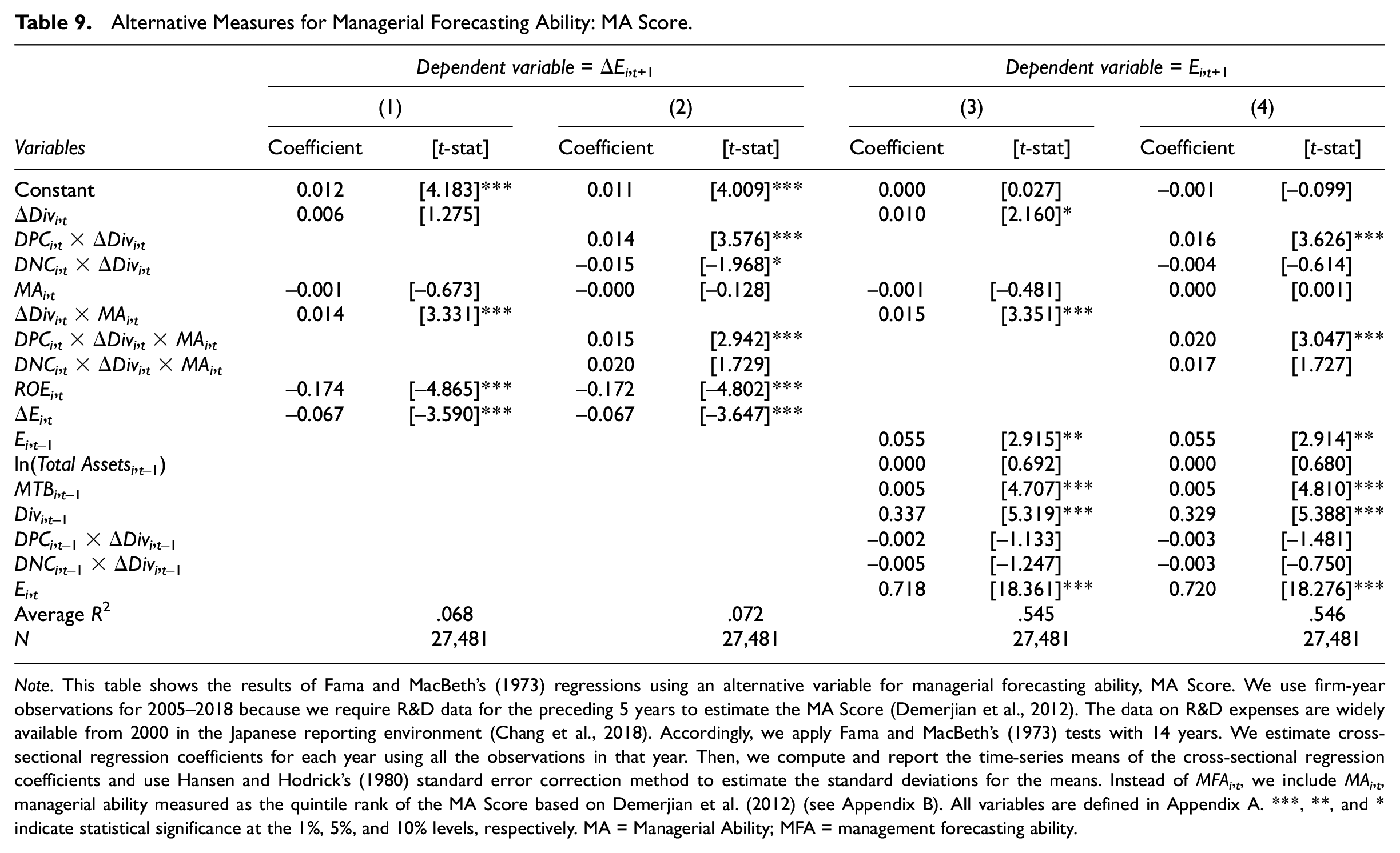
Note. This table shows the results of Fama and MacBeth’s (1973) regressions using an alternative variable for managerial forecasting ability, MA Score. We use firm-year observations for 2005–2018 because we require R&D data for the preceding 5 years to estimate the MA Score (Demerjian et al., 2012). The data on R&D expenses are widely available from 2000 in the Japanese reporting environment (Chang et al., 2018). Accordingly, we apply Fama and MacBeth’s (1973) tests with 14 years. We estimate cross-sectional regression coefficients for each year using all the observations in that year. Then, we compute and report the time-series means of the cross-sectional regression coefficients and use Hansen and Hodrick’s (1980) standard error correction method to estimate the standard deviations for the means. Instead of MFAi, t , we include MAi, t , managerial ability measured as the quintile rank of the MA Score based on Demerjian et al. (2012) (see Appendix B). All variables are defined in Appendix A. ***, **, and * indicate statistical significance at the 1%, 5%, and 10% levels, respectively. MA = Managerial Ability; MFA = management forecasting ability.
Conclusion
In this study, we revisit the predictive ability of dividend changes for future earnings and enhance the literature by examining the effect of management forecasting ability. Although prior literature has examined the implications of dividend changes for future earnings, the empirical evidence has been largely mixed. In this regard, we anticipate that the predictive ability of dividend changes depends on managers’ forecasting ability and posit that dividend changes have a positive association with firms’ future earnings, particularly when managers are good at assessing future earnings. The original framework of Lintner (1956) and Miller and Modigliani (1961) assumes that well-informed managers can correctly assess future earnings prospects and signal the implication through increased or decreased dividend payouts. We use this theoretical assumption and investigate whether managerial forecasting ability affects the linkage between dividend changes and future earnings.
Using a sample of Japanese dividend-paying firms, we first observe that dividend changes, particularly dividend increases, are significantly and positively associated with earnings changes and earnings levels in the following year. We then find that management forecasting ability has a moderating effect on the predictive ability of dividends. Specifically, dividend changes made by managers with high-forecasting ability are more likely to be positively associated with firms’ future earnings. These results are robust to various sensitivity tests, including partitioned subsamples regression analysis, Theil-Sen regression approach, alternative variable scalers, and alternative measurements of managers’ forecasting ability. Overall, our results support the predictive ability of dividend changes and suggest that the linkage between dividend changes and future earnings is more pronounced for firms with high-forecasting ability managers.
Footnotes
Appendix B
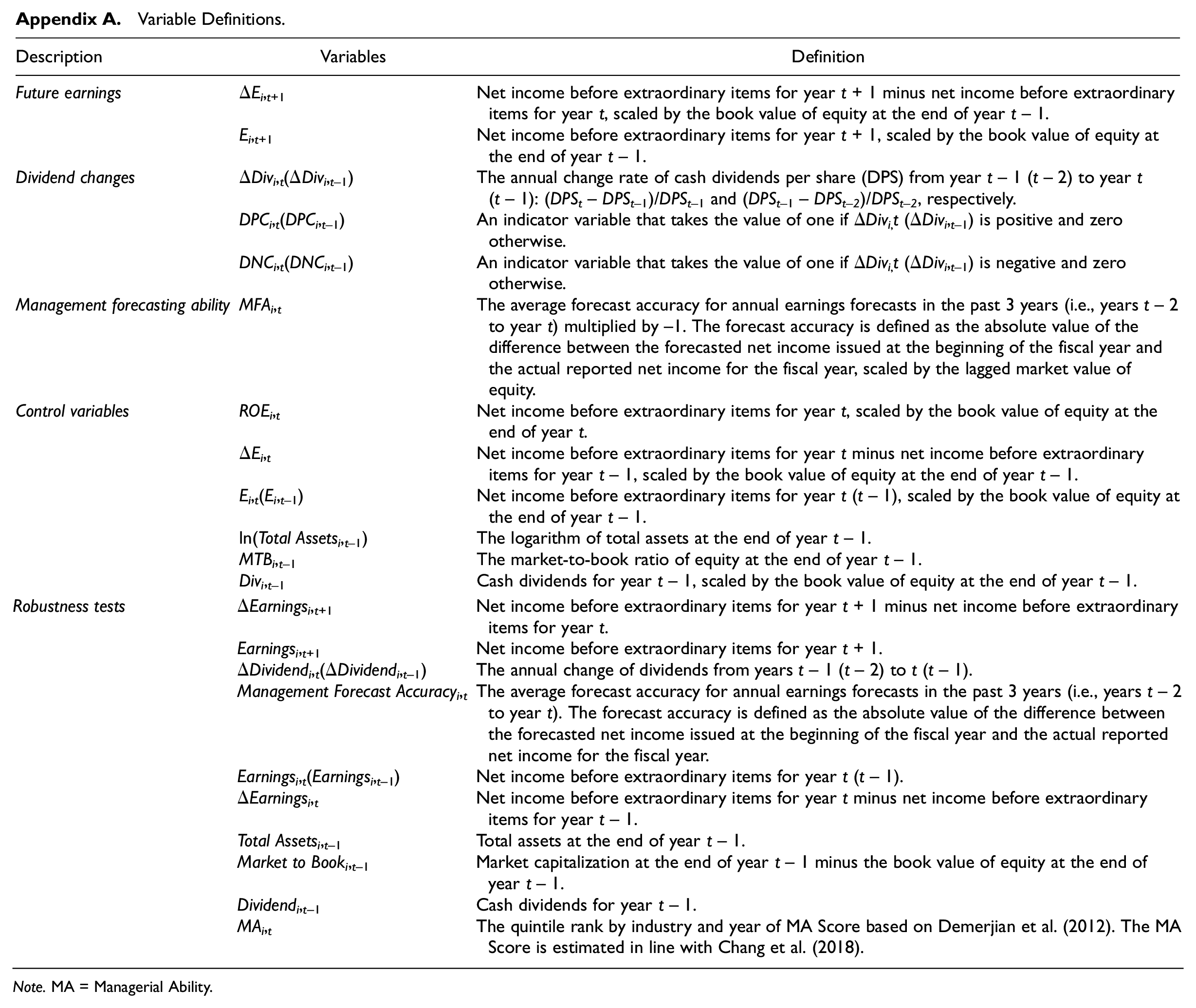
Appendix A.
Variable Definitions.
| Description | Variables | Definition |
|---|---|---|
| Future earnings | ΔEi,t+1 | Net income before extraordinary items for year t+ 1 minus net income before extraordinary items for year t, scaled by the book value of equity at the end of year t− 1. |
| Ei,t+1 | Net income before extraordinary items for year t+ 1, scaled by the book value of equity at the end of year t− 1. | |
| Dividend changes | ΔDivi,
t
(ΔDivi,t−1) |
The annual change rate of cash dividends per share (DPS) from year t− 1 (t− 2) to year t (t− 1): (DPSt−DPSt−1)/DPSt−1 and (DPSt−1−DPSt−2)/DPSt−2, respectively. |
| DPCi,
t
(DPCi,t−1) |
An indicator variable that takes the value of one if ΔDivi,t (ΔDivi,t−1) is positive and zero otherwise. | |
| DNCi,
t
(DNCi,t−1) |
An indicator variable that takes the value of one if ΔDivi,t (ΔDivi,t−1) is negative and zero otherwise. | |
| Management forecasting ability | MFAi, t | The average forecast accuracy for annual earnings forecasts in the past 3 years (i.e., years t− 2 to year t) multiplied by −1. The forecast accuracy is defined as the absolute value of the difference between the forecasted net income issued at the beginning of the fiscal year and the actual reported net income for the fiscal year, scaled by the lagged market value of equity. |
| Control variables | ROEi, t | Net income before extraordinary items for year t, scaled by the book value of equity at the end of year t. |
| ΔEi, t | Net income before extraordinary items for year t minus net income before extraordinary items for year t− 1, scaled by the book value of equity at the end of year t− 1. | |
| Ei,
t
(Ei,t−1) |
Net income before extraordinary items for year t (t− 1), scaled by the book value of equity at the end of year t− 1. | |
| ln(Total Assetsi,t−1) | The logarithm of total assets at the end of year t− 1. | |
| MTBi,t−1 | The market-to-book ratio of equity at the end of year t− 1. | |
| Divi,t−1 | Cash dividends for year t− 1, scaled by the book value of equity at the end of year t− 1. | |
|
Robustness
tests |
ΔEarningsi,t+1 | Net income before extraordinary items for year t+ 1 minus net income before extraordinary items for year t. |
| Earningsi,t+1 | Net income before extraordinary items for year t+ 1. | |
| ΔDividendi,
t
(ΔDividendi,t−1) |
The annual change of dividends from years t− 1 (t− 2) to t (t− 1). | |
| Management Forecast Accuracyi, t | The average forecast accuracy for annual earnings forecasts in the past 3 years (i.e., years t− 2 to year t). The forecast accuracy is defined as the absolute value of the difference between the forecasted net income issued at the beginning of the fiscal year and the actual reported net income for the fiscal year. | |
| Earningsi,
t
(Earningsi,t−1) |
Net income before extraordinary items for year t (t− 1). | |
| ΔEarningsi, t | Net income before extraordinary items for year t minus net income before extraordinary items for year t− 1. | |
| Total Assetsi,t−1 | Total assets at the end of year t− 1. | |
| Market to Booki,t−1 | Market capitalization at the end of year t− 1 minus the book value of equity at the end of year t− 1. | |
| Dividendi,t−1 | Cash dividends for year t− 1. | |
| MAi, t | The quintile rank by industry and year of MA Score based on Demerjian et al. (2012). The MA Score is estimated in line with Chang et al. (2018). |
Note. MA = Managerial Ability.
Acknowledgements
We thank Bharat Sarath (Editor in Chief), Pradyot K. Sen (Associate Editor), and an anonymous reviewer for their constructive comments and suggestions for our manuscript. We also thank helpful comments from Rajiv Banker, Mark Anderson, Kentaro Koga, Makoto Nakano, Akinobu Shuto, Tetsuyuki Kagaya, Takashi Ebihara, Ryosuke Nakamura, and conference and workshop participants at the 2019 European Accounting Association Annual Congress, the 2019 International Conference on Data Envelopment Analysis, the 2018 Japanese Accounting Association Annual Conference, the 2018 Japan Academic Society of Investor Relations Annual Conference, Hitotsubashi University, National Taipei University, and National Chung Hsin University. We gratefully acknowledge the financial support from the Grant-in-Aid for Scientific Research from the Ministry of Education, Culture, Sports, Science, and Technology of Japan (ID: 19K13848). All errors remain ours.
Declaration of Conflicting Interests
The author(s) declared no potential conflicts of interest with respect to the research, authorship, and/or publication of this article.
Funding
The author(s) disclosed receipt of the following financial support for the research, authorship, and/or publication of this article: This work was supported by the Grant-in-Aid for Scientific Research from the Ministry of Education, Culture, Sports, Science, and Technology of Japan (ID: 19K13848).
Data Availability
All data used in the study is from publicly available sources cited in the text.