
Abstract
The dicentric chromosome assay (DCA) serves as the gold standard for quantifying ionising radiation exposure in individuals. However, the conventional manual scoring method for DCA is both time-consuming and mentally demanding. Consequently, numerous research groups and commercial entities are actively pursuing the integration of artificial intelligence to automate this process. In this study, we present methodologies and techniques employed at the Singapore Nuclear Research and Safety Initiative (SNRSI) for the development and optimisation of an in-house automated dicentric chromosome scoring tool. Our approach involves the utilisation of thresholding and watershed methods to identify chromosomes within a metaphase. Subsequently, these identified chromosomes are fed into a trained convolutional neural network (CNN) for classification and centromere number assignment. The cumulative centromere count is then calculated to determine the acceptance or rejection of the metaphase for scoring. This integration of advanced image processing techniques and machine learning algorithms would streamline and enhance the efficiency of the dicentric chromosome scoring at SNRSI.
INTRODUCTION
The dicentric chromosome assay (DCA) is a well-established method crucial in triage, providing a means to quantify the ionising radiation dose for individuals exposed, enabling the prescription of appropriate treatments. The enumeration of dicentric chromosomes in the first-division metaphase of peripheral blood lymphocytes serves as a reliable indicator of radiation exposure (Wong et al., 2013). Conventionally, determining the dicentric chromosome per cell ratio from a metaphase image requires one to first identify ideally spread chromosomes in an image; count the number of centromeres of each chromosome; determine if the chromosome is monocentric, dicentric, or an acentric fragment; and finally sum the total number of centromeres present in the metaphase image to accept or reject a metaphase. Based on the International Atomic Energy Agency (IAEA) 2011 publication (IAEA, 2011), metaphases should ideally exhibit 46 centromeres, although some biodosimetry laboratories accept metaphases with 45 centromeres (Endesfelder et al., 2023). This manual scoring process is time-consuming, hindering efficient dose estimation.
Automation emerges as a solution to reduce the considerable man-hours required for dose estimation. Existing automated scoring software, such as commercial solutions like DCScore (MetaSystems GmbH, Altlussheim, Germany), Automated Dicentric Chromosome Identifier and Dose Estimator (ADCI) (Shirley et al., 2017) and tools developed by research groups like the image analysis software FluorQuantDic used with Rapid Automated Biodosimetry Tool II (Royba et al., 2019) and deep learning-based systems (Jang et al., 2021), are available. However, these solutions can be expensive and may not be feasible for smaller, lower-throughput labs. Consequently, developing an in-house automated dicentric counting software offers a customisable alternative, accommodating specific requirements and providing flexibility in making changes to the features in the software.
This article showcases the various models and techniques the Singapore Nuclear Research and Safety Initiative (SNRSI) employed to create and optimise the in-house automated dicentric chromosome scoring tool. The process initiates with data mining of metaphase images to label chromosomes and dicentrics, creating the necessary training data. Subsequently, various optimiser algorithms and neural network architectures from TensorFlow are utilised to build a prediction model capable of accurately classifying monocentric chromosomes, dicentric chromosomes, and acentric fragments, ultimately facilitating radiation dose estimation.
2. SCORING
The automated scoring system was developed using Python 3 (Van Rossum and Drake, 1995), leveraging the computer vision module OpenCV (Bradski, 2000) to facilitate chromosome identification within images. Employing machine learning modules TensorFlow (Abadi et al., 2015) and Keras (Chollet et al., 2015), neural networks were created and trained to classify chromosomes as monocentric, dicentric, or acentric fragments. Metaphase images, captured by the Metafer 4 system version 3.12.7 (MetaSystems GmbH, Altlussheim, Germany) and exported in .TIF format, served as input. OpenCV, employing a combination of thresholding and watershed methods (Kornilov and Safonov, 2018), discerned individual chromosomes from the background. Chromosomes identified were then cropped along their contours and resized to 28 pixels by 28 pixels, retaining crucial information for centromere recognition while optimising computational efficiency. The resized chromosome images were input into a pretrained convolutional neural network (CNN) model, which classified each chromosome as monocentric, dicentric, or a fragment, assigning centromere numbers 1, 2, and 0, respectively. Postclassification, the system tallied the total centromere count in the metaphase image, rejecting images with fewer than 45 or more than 46 centromeres. The dicentric per cell ratio was subsequently tabulated, providing an estimate of the received radiation dose.
2.1. Thresholding and watershed method
The process of identifying chromosomes from the background involved the strategic use of thresholding and the watershed method. The threshold value for each image was algorithmically determined, with the initial adoption of the OTSU method (Otsu, 1979) to establish a benchmark threshold for identifying chromosomes within the image. The area of each threshold-identified object was measured and considered a valid chromosome if it fell within a specified range. In cases where the object's area deviated outside this range, the watershed algorithm was subsequently applied. This algorithm, based on the object’s texture, effectively partitioned it into smaller objects if multiple boundaries were detected. Objects were rejected if the watershed algorithm identified them as a single, large-area boundary surpassing a predefined value, thereby distinguishing stained debris from overlapping chromosomes.
Following the identification of all chromosomes in the metaphase image, the algorithm conducted a validation check to ensure an optimal threshold value was chosen. OTSU method threshold values yielding centromere counts between 44 and 47 were accepted. Alternatively, the system iteratively explored other threshold values, selecting the one that yielded a chromosome count closest to the ideal target of 46 centromeres. This approach ensured the accurate identification of chromosomes and the selection of optimal threshold values for subsequent analyses (Fig. 1).
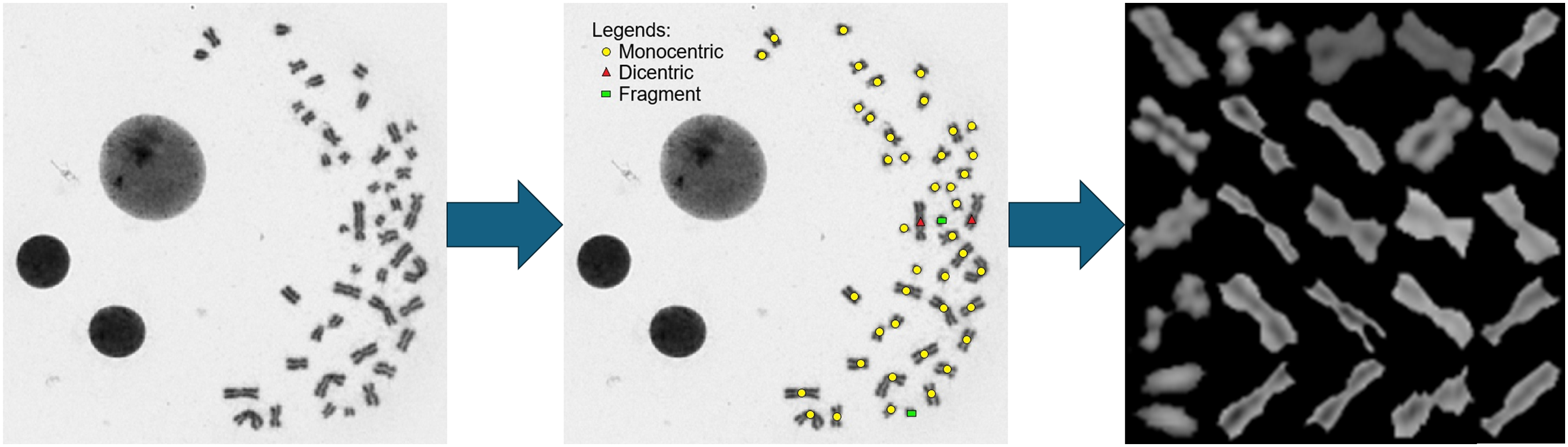
Illustration of the image processing process. Metaphase image is input into the system, where individual chromosomes are identified by thresholding and watershed method, and finally cropped into individual 28 pixels by 28 pixels chromosome images to be further categorised by the neural network. In the middle image, yellow dots mark monocentric chromosomes assigned with a centromere number 1, red triangles label dicentric chromosomes with a centromere number of 2, and green rectangles mark acentric fragments with a centromere number of 0.
2.2. Artificial intelligence
2.2.1. Deep learning model
CNN were employed in the automation process, leveraging their inherent capability to classify images through pattern recognition of pixel data. Our model adopted an architecture inspired by VGGNet (Simonyan and Zisserman, 2014), employing a kernel size of three pixels by three pixels. This choice was motivated by the simplicity and effectiveness of increasing the number of convolutional layers, contributing to the development of a robust model.
To enhance the model's performance, a double convolutional layer stacked consecutively was identified as yielding the highest verification accuracy for our dataset. This configuration facilitated the extraction of more complex features without succumbing to overfitting, as observed in models with three consecutive convolutional layers where the accuracy was reduced by 13%. The utilisation of average pooling accommodates both dark and light background images, ensuring a comprehensive representation of features. The complete architecture of our CNN model is illustrated in Fig. 2.
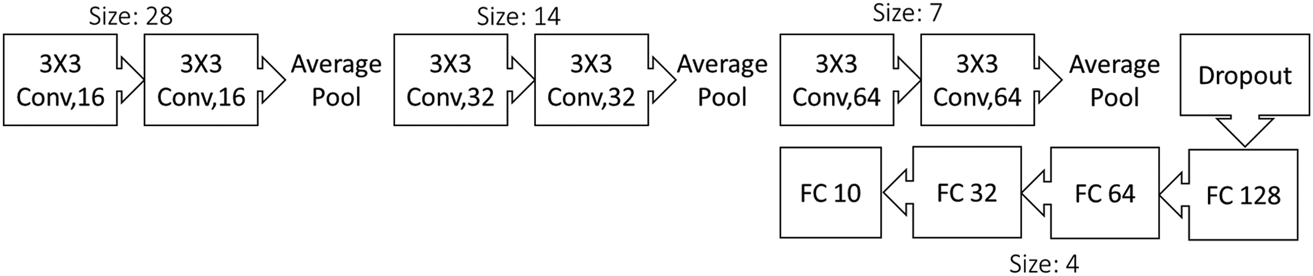
Convolutional neural network architecture based on VGGNet architecture used for our neural network model. The model incorporates double convolutional layers with a kernel size of three pixels by three pixels. Each subsequent double convolutional layer (Conv) introduces an increasing number of feature maps, contributing to the model's capacity to discern intricate patterns. The model ends with four fully connected layers (FC) with diminishing number of channels, with a final 10 classes to accommodate for future uses.
2.2.2. Training data
We extracted 28 pixels by 28 pixels chromosome images from scored metaphases, labelled by our scorers who have achieved ±0.5 Gy accuracy in at least three interlaboratory comparisons. These labelled images served as the foundation of our training dataset. The dataset comprised a total of 28,005 labelled chromosome images, encompassing monocentric chromosomes, dicentric chromosomes, and acentric fragments, which were utilised for both model training and validation. Ninety percent of the dataset was allocated for the training process, while the remaining 10% was reserved for validation purposes. The dataset underwent augmentation to enhance its diversity, incorporating random flip and random rotation. This augmentation effectively doubled the dataset size to a total of 56,010 images, with 50,410 images designated for training and 5600 images earmarked for validation.
2.2.3. Model accuracy
The model's validation accuracy is determined by assessing its ability to accurately predict the remaining 10% of chromosome images designated for validation. For instance, a 90% accuracy implies that the model correctly labelled 5040 out of the 5600 validation images. It is crucial to emphasise that this accuracy value pertains specifically to the individual chromosome level and does not reflect the accuracy of the dose estimation process.
2.2.4. Optimisers
During the training phase, CNN optimisers played a crucial role in adjusting the weights and learning rates of neurons to enhance the model's accuracy. Several optimisers available in the Keras environment were systematically evaluated to identify the most effective choice for our dataset. After rigorous testing, Adamax emerged as the optimal optimiser, achieving a validation accuracy of 91.04%.
The ranking of the tested optimisers, ordered by decreasing validation accuracy, is as follows: Adamax led the list with 91.04%, followed by Adam at 80.97%, and Nadam also at 80.97%. Subsequently, Adagrad achieved a validation accuracy of 77.62%, while the ranking continued with root mean square propagation at 55.47%, stochastic gradient descent at 54.47%, and finally, follow the regularised leader at 51.56%.
3. DOSE ESTIMATION
3.1. Calibrating the curve
We constructed a dose–response curve for dose estimation, utilising the dicentric per cell ratio evaluated by the trained CNN model for doses equal to or greater than 1 Gy. To be considered for dose estimation, a metaphase image must satisfy specific criteria, requiring the presence of 45 or 46 centromeres and fewer than five dicentrics, as identified by the CNN model. Each dose point in the curve was based on a selection of at least 1000 metaphases meeting these criteria, apart from the 5 Gy data point, which had at least 250 dicentrics. The data was fitted to a second-order quadratic equation:

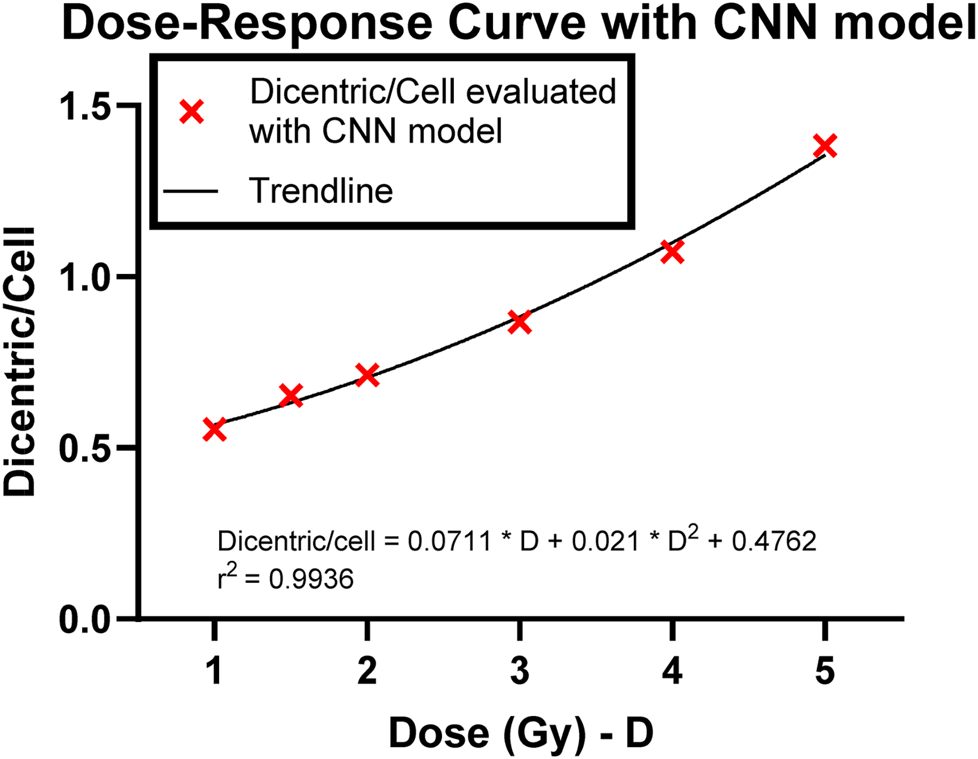
Dose–response curve built using CNN model. The X markers represent the dicentric cell per count evaluated with the CNN model, while the line represents the quadratic fitting of the data points.
3.2. Testing the calibration curve
The CNN model underwent additional testing on metaphase images that were neither part of the model training dataset nor involved in calibrating the dose–response curve. This testing involved irradiated samples with five distinct doses, ranging from 1 to 5 Gy, encompassing approximately 500 images for each dose. The model efficiently processed 500 images within a timeframe of approximately 30 min.
The estimated dose for each sample was subsequently calculated by leveraging the dicentric per cell count predicted by the CNN model. This count was then matched to the corresponding dose on the established dose–response curve illustrated in Fig. 3. The resultant estimated doses demonstrated a remarkable accuracy, falling within a range of ±0.5 Gy from the actual doses. These findings are visually presented in Fig. 4.
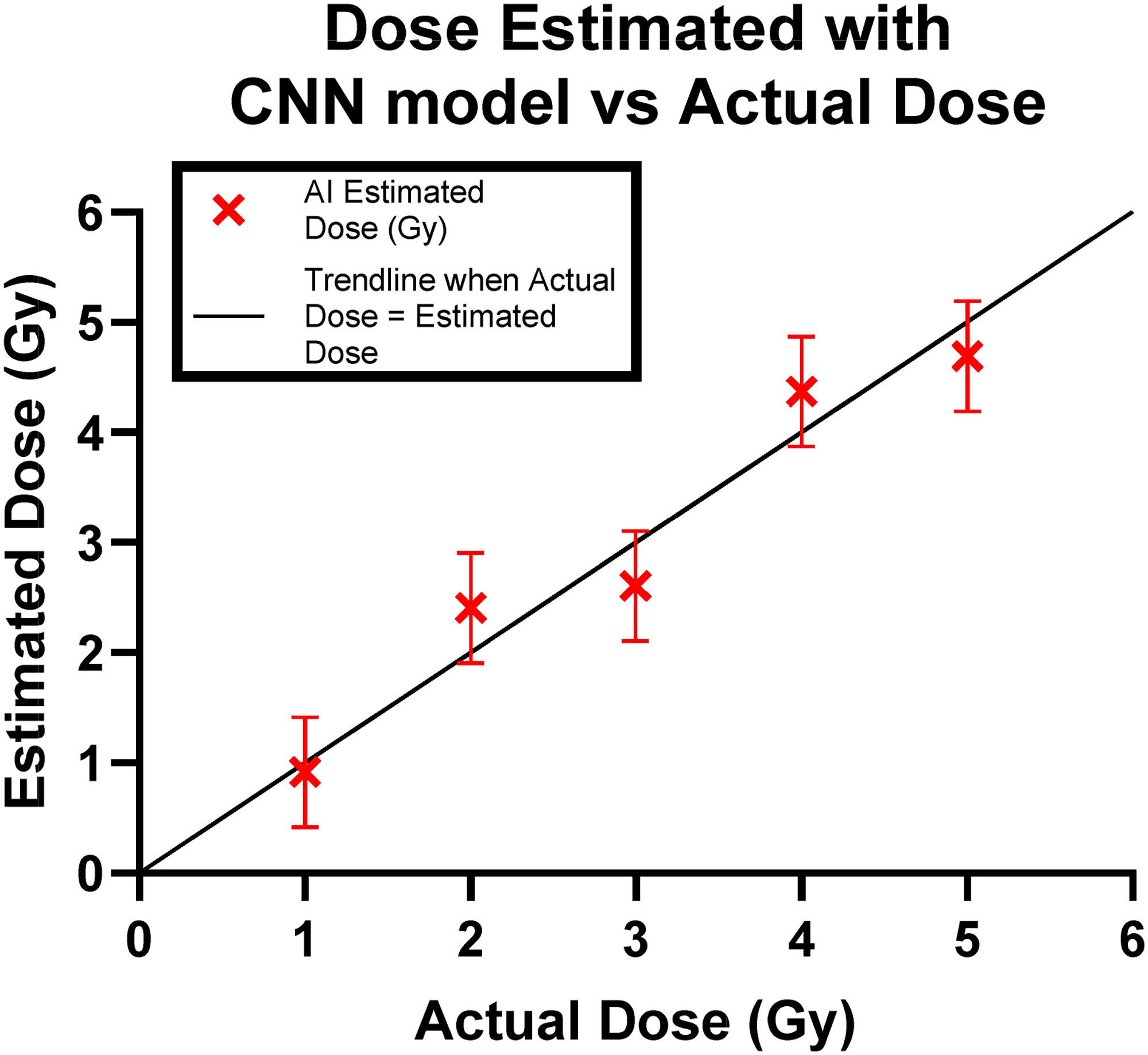
Verification of dose estimation of the CNN model. Error bars show a ±0.5Gy range.
3.3. Limitations and future improvements
The prevailing constraint of the current model is attributed to a notable correction factor, specifically the elevated value of 0.4762 for dicentric per cell. This high correction factor is a consequence of the CNN model's validation accuracy. The challenge arises from the need to validate 46 chromosomes per cell. Having a 90% accuracy at the chromosome level translates to a classification error possibly occurring approximately every two metaphases assessed. A potential remedy to mitigate this challenge involves adopting a multi-model approach, wherein multiple models are concurrently deployed to verify a single image. The rationale behind this strategy is rooted in the theory that employing several models for verification would diminish the likelihood of simultaneous false classifications by multiple models for the same chromosome.
4. CONCLUSION
This study presents the exploratory integration of artificial intelligence into the dicentric chromosome assay scoring process for efficient and accurate dose estimation in radiation-exposed individuals at SNRSI. The calibration of the dose–response curve and its testing on metaphase images demonstrate the model's ability to provide accurate dose estimations within a ±0.5 Gy range. However, there are limitations with the software, notably the high correction factor influenced by the validation accuracy, resulting in challenges in quantifying radiation doses below 1 Gy. A potential solution involves a multi-model approach to minimise false classifications, presenting a promising avenue for future improvements. The article concludes with ongoing enhancements to the automation software and improvements to the model's accuracy.
Footnotes
DECLARATION OF CONFLICTING OF INTEREST
The authors declared no potential conflicts of interest with respect to the research, authorship, and/or publication of this article.
FUNDING
The authors disclosed receipt of the following financial support for the research, authorship, and/or publication of this article: This research was funded by the National Research Foundation, Singapore.