ICRP Publication 133: The ICRP computational framework for internal dose assessment for reference adults: specific absorbed fractions

Editorial

SPECIFIC ABSORBED FRACTIONS: A KEY STEP IN CALCULATION OF INTERNAL DOSE

I recall learning how to calculate doses due to internal exposure during my graduate work in medical physics at McMaster University in Hamilton, Ontario, Canada. I remember being fascinated by the biokinetic models used to trace the fate of inhaled or ingested radionuclides, and the concept of specific absorbed fractions; this despite a generally fallible memory. I remember the classroom, the exercises done on the chalkboard (no iPads back then!), and, most of all, I remember the sense of wonder at such a clever and sophisticated, yet conceptually simple, set of ideas behind assessing the dose to each of the organs and tissues in the human body. How is it that lessons from decades ago are etched so clearly in the mind, when some memories of last week, or even yesterday, fade so quickly?

At the time I knew very little about the mysterious (to me) International Commission on Radiological Protection (ICRP), and even less about the eminent people behind it. I thought I understood radiological protection, but now I know that I had barely scratched the surface.

Calculation of internal dose is one of the most sophisticated aspects of radiological protection. Equivalent doses to organs and tissues cannot be measured directly, and no operational quantities (measurable physical quantities) exist to stand in their place. Instead, a mathematical assessment is necessary based fundamentally on an estimate of the activity of radionuclide intake, mainly by inhalation or ingestion when considering worker and public exposures (also by absorption through the skin for the water form of tritium), but also by direct injection for use in medical practice. Often, the activity of a radionuclide taken into the body is not well known, and so it is back-calculated based on bioassay results (e.g. urinalysis). The path of a radionuclide is traced through the body over time, and radiation doses to each of the organs and tissues are calculated based on these modelling assumptions.

Note that an internal dose is always a committed dose. A committed dose is one that will be received over time as a result of radionuclides residing inside the body. Depending on the physical half-life of the radionuclide (how quickly it decays), and the biological half-life of the specific chemical form (how quickly it passes through the body), the majority of the dose could be delivered within hours or less, or it could take decades. For protection purposes, for comparison with dose limits, reference levels, and constraints, the committed dose is counted when the radionuclide is taken into the body. For adults, the dose is calculated over a period of 50 years following exposure, while for children, it is calculated to 70 years of age.

This is one key difference from external radiation fields where organ doses are received from exposure to a source outside the body when a radioactive source is nearby. When the source is taken away, the exposure stops. For internal exposures, the source cannot be ‘taken away’ in the same sense as it has been incorporated into the body, and so the exposure continues.

If all of this sounds a bit complicated, that is because it is. However, ICRP has done the ‘heavy lifting’, calculating the committed dose per unit intake for inhalation and ingestion of a wide variety of radionuclides of various chemical forms and particle sizes.

Results are summarised as effective dose coefficients (in Sv Bq^–1), which, when multiplied by the activity intake (Bq), provide the committed effective dose (Sv). When more detail is needed, similar coefficients, also produced by ICRP, can be used to calculate the committed equivalent doses to individual organs and tissues over different time periods.

But where do these effective dose coefficients come from? Many ingredients are needed, including: nuclear decay data [Publication 107 (ICRP, 2008)], biokinetic models [e.g. Publication 130 (ICRP, 2015)], anatomical and physical data [Publication 89 (ICRP, 2002)], and computational phantoms [e.g. Publication 110 (ICRP, 2009)].

Biokinetic models are used to calculate the distribution of an inhaled or ingested radionuclide among organs and tissues over time. Nuclear decay data provide information on the radiation emitted by these radionuclides. However, radiation emitted from a radionuclide in an organ is not always fully absorbed by that ‘source’ organ.

Computational phantoms and anatomical and physical data are used to calculate absorbed fractions: the fraction of radiation energy emitted from a source organ that is absorbed in a target organ. This takes an enormous amount of expertise, time, and computational power, using Monte Carlo radiation transport codes with the complex geometries of the computational phantoms, many radiation types and energies, and many combinations of source and target organs.

The specific absorbed fraction (SAF) is the absorbed fraction divided by the mass of the target tissue, and expressed in units of kg⁻¹. For example, for 1 MeV photons emitted from the male liver, approximately 0.79% of the energy emitted is absorbed in the left and right kidneys. As the mass of the male left and right kidneys given in Table A.1 is 0.422 kg, the specific absorbed fraction is 0.0079/0.422 kg = 0.019 kg⁻¹. Similar calculations are undertaken for alpha and beta particles, photons, and neutrons of various energies. Their emission and subsequent energy absorption is modelled in all combinations of source regions and target tissues in both the male and female phantoms, as both are needed in the calculation of effective doses to Reference Person.

Once you know where the radionuclides are in the body and the radiations they are emitting, the SAFs make the calculation of absorbed doses to all of the organs and tissues relatively straightforward, although even this would have been a challenge a few decades ago when computers were not in common use.

At this point, absorbed doses to the organs of the adult male and female reference phantoms are averaged to get absorbed doses to Reference Person. Equivalent doses to organs are calculated by multiplying the absorbed doses to organs by the radiation weighting factors, and the effective dose is calculated by summing the equivalent doses to organs multiplied by the tissue weighting factors.

The current publication provides information on the methodology of calculating SAFs, as well as the results for the adult male and adult female reference phantoms. The Occupational Intakes of Radionuclides (OIR) series of reports, of which Publication 130 (ICRP, 2015) is the first, goes one step further and presents the dose coefficients for a large number of radionuclides.

The results of the calculations outlined above are as enormous as the effort that has gone into producing them. The previous series of OIR reports [Publication 30 series (ICRP, 1979a,b, 1980, 1981a,b, 1982a,b,c, 1988)], published in nine parts between 1979 and 1988, amounted to nearly 4000 pages of printed text, the vast majority of which were tables of numbers. For the last few decades, CDs were produced for these and other ICRP publications that include large data sets. Some of these CDs were included in the relevant publication, while others were distributed separately.

However, CDs have limitations. They are relatively expensive to produce, difficult to update, and many computers do not even come equipped with CD drives nowadays. So, having entered the Internet Age, ICRP is now distributing large data sets, and, in some cases, software that uses them, via the Internet. These will be available through the ICRP website, as well as the website of the publisher of the Annals of the ICRP, SAGE UK. In both cases, the files will be found on the same pages as the relevant publications. To ease access, the datasets will be free to download, even if the publications themselves still need to be purchased.

For the current publication, Annex B describes the electronic files and notes that they are downloadable from www.icrp.org. Our intention is that each publication with associated data files will have a similar annex describing the files and pointing readers to their location.

Knowing the enormous amount of expertise and time that goes into calculating (and double- and triple-checking) the SAFs and all of the dose coefficients for internal exposure, one cannot help but be impressed by the work of the authors of this report.

Moreover, these SAFs and the OIR series of reports are far from the end of the story. A similar effort is ongoing for doses to members of the public. This is even more complex than for occupational exposures, as the reference phantoms are not limited to adults. A set of paediatric reference phantoms, both male and female, has been adopted, as has a set of reference phantoms for the pregnant female and fetus at various stages of development. Work is underway to calculate SAFs for these phantoms, and ultimately dose coefficients for members of the public. All of this will appear in future ICRP publications.

CHRISTOPHER H. CLEMENT

ICRP SCIENTIFIC SECRETARY

EDITOR-IN-CHIEF

REFERENCES

ICRP, 1979a. Limits for intakes of radionuclides by workers. ICRP Publication 30 (Part 1). Ann. ICRP 2(3/4). a-5 ICRP, 1979b. Limits for intakes of radionuclides by workers. ICRP Publication 30 (Supplement to Part 1). Ann. ICRP 3(1–4). a-6 ICRP, 1980. Limits for intakes of radionuclides by workers. ICRP Publication 30 (Part 2). Ann. ICRP 4(3/4). a-7 ICRP, 1981a. Limits for intakes of radionuclides by workers. ICRP Publication 30 (Supplement to Part 2). Ann. ICRP 5(1–6). a-8 ICRP, 1981b. Limits for intakes of radionuclides by workers. ICRP Publication 30 (Part 3). Ann. ICRP 6(2/3). a-9 ICRP, 1982a. Limits for intakes of radionuclides by workers. ICRP Publication 30 (Supplement A to Part 3). Ann. ICRP 7(1–3). a-10 ICRP, 1982b. Limits for intakes of radionuclides by workers. ICRP Publication 30 (Supplement B to Part 3). Ann. ICRP 8(1–3). a-11 ICRP, 1982c. Limits for intakes of radionuclides by workers. ICRP Publication 30 (Index). Ann. ICRP 8(4). a-12 ICRP, 1988. Limits for intakes of radionuclides by workers: an addendum. ICRP Publication 30 (Part 4). Ann. ICRP 19(4). a-13 ICRP, 2002. Basic anatomical and physiological data for use in radiological protection reference values. ICRP Publication 89. Ann. ICRP 32(3/4). a-2 ICRP, 2008. Nuclear decay data for dosimetric calculations. ICRP Publication 107. Ann. ICRP 38(3). a-0 ICRP, 2009. Adult reference computational phantoms. ICRP Publication 110. Ann. ICRP 39(2). a-3 ICRP, 2015. Occupational intakes of radionuclides: Part 1. ICRP Publication 130. Ann. ICRP 44(2). a-1a-4

The ICRP computational framework for internal dose assessment for reference adults: specific absorbed fractions

Approved by the Commission in May 2016

Abstract–Dose coefficients for assessment of internal exposures to radionuclides are radiological protection quantities giving either the organ equivalent dose or effective dose per intake of radionuclide following ingestion or inhalation. In the International Commission on Radiological Protection’s (ICRP) Occupational Intakes of Radionuclides (OIR) publication series, new biokinetic models for distribution of internalised radionuclides in the human body are presented as needed for establishing time-integrated activity within organs of deposition (source regions). This series of publications replaces Publications 30 and 68 (ICRP, 1979, 1980, 1981, 1988, 1994b). In addition, other fundamental data needed for computation of the dose coefficients are radionuclide decay data (energies and yields of emitted radiations), which are given in Publication 107 (ICRP, 2008), and specific absorbed fraction (SAF) values – defined as the fraction of the particle energy emitted in a source tissue region that is deposited in a target tissue region per mass of target tissue. This publication provides the technical basis for SAFs relevant to internalised radionuclide activity in the organs of Reference Adult Male and Reference Adult Female as defined in Publications 89 and 110 (ICRP, 2002, 2009). SAFs are given for uniform distributions of mono-energetic photons, electrons, alpha particles, and fission-spectrum neutrons over a range of relevant energies. Electron SAFs include both collision and radiative components of energy deposition. SAF data are matched to source and target organs of the biokinetic models of the OIR publication series, as well as the Publication 100 (ICRP, 2006) Human Alimentary Tract Model and the Publication 66 (ICRP, 1994a) Human Respiratory Tract Model, the latter as revised within Publication 130 (ICRP, 2015). This publication further outlines the computational methodology and nomenclature for assessment of internal dose in a manner consistent with that used for nuclear medicine applications. Numerical data for particle-specific and energy-dependent SAFs are given in electronic format for numerical coupling to the respiratory tract, alimentary tract, and systemic biokinetic models of the OIR publication series.

© 2016 ICRP. Published by SAGE.

Keywords: Computational phantom; Absorbed fraction; Specific absorbed fraction; Radiation transport; Internal dosimetry

AUTHORS ON BEHALF OF ICRP

W.E. BOLCH, D. JOKISCH, M. ZANKL,

K.F. ECKERMAN, T. FELL, R. MANGER, A. ENDO,

J. HUNT, K.P. KIM, N. PETOUSSI-HENSS

PREFACE

The membership of Task Group 96 on Computational Phantoms and Radiation Transport at the time of completion of this publication was:

W.E. Bolch (Chairman)	D. Jokisch	N. Petoussi-Henss
A. Endo	C.H. Kim	M. Zankl
J.G.S. Hunt	C. Lee

The corresponding members were:

K.F. Eckerman	J. Li
K.P. Kim	H. Schlattl

The membership of Task Group 95 on Internal Dose Coefficients at the time of completion of this publication was:

F. Paquet (Chairman)	E.J.A. Blanchardon	A. Giussani
M.R. Bailey	G. Etherington	R.W. Leggett
V. Berkovskyy	T. Fell

The corresponding members were:

E. Ansoborlo	J. Marsh	G. Ratia
L. Bertelli	D. Melo	T. Smith
E. Davesne	D. Nosske
D. Gregoratto	M. Puncher

The membership of Committee 2 during the period of preparation of this publication was:

(2009–2013)

H-G. Menzel (Chairman)	R. Cox	R. Leggett
M.R. Bailey	G. Dietze	J.L. Lipsztein
M. Balonov	K.F. Eckerman	J. Ma
D. Bartlett	A. Endo	F. Paquet
V. Berkovskyy	J.D. Harrison	N. Petoussi-Henss
W.E. Bolch	N. Ishigure	A.S. Pradhan

(2013–2017)

J.D. Harrison (Chairman)	M. Degteva	D. Nosske
M.R. Bailey	A. Endo	F. Paquet
V. Berkovskyy	J.G.S. Hunt	N. Petoussi-Henss
L. Bertelli	C. Hyeong Kim	F. Wissmann
W.E. Bolch	R. Leggett
D. Chambers	J. Ma

Acknowledgements

Helpful comments from Main Commission members H-G. Menzel and J-K. Lee, as well as continued assistance by the former Associate Editor N. Hamada are gratefully acknowledged.

Main Points

Dose coefficients for assessment of internal exposure to radionuclides following inhalation and ingestion require the use of biokinetic models [Publication 130 (ICRP, 2015)], radionuclide decay scheme data [Publication 107 (ICRP, 2008)], and specific absorbed fraction (SAF) values in a computational phantom.

SAFs are defined as the fraction of particle energy emitted in a source region that is deposited in a target region per mass of target tissue, and are expressed in units of kg⁻¹.

This publication presents reference values of the SAFs for internally emitted photons, electrons, and alpha particles, as well as fission-spectrum neutrons associated with radionuclides that decay by spontaneous fission.

The majority of SAF values given in this publication are derived from Monte Carlo radiation transport simulations in Reference Adult Male and Reference Adult Female computational phantoms defined in Publication 110 (ICRP, 2009).

Additional SAF values for electron and alpha particles are taken from Publication 66 (ICRP, 1994a) for the Human Respiratory Tract Model (HRTM), with changes consistent with revisions to the HRTM presented in Publication 130 (ICRP, 2015).

In this publication, new SAF values for electron and alpha particles are given for the Human Alimentary Tract Model (HATM) that supercede those given in Publication 100 (ICRP, 2006).

The reference SAFs presented in this publication are numerically coupled to the compartmental models of the HRTM, HATM, and the systemic biokinetic models of Publication 130 (ICRP, 2015) in the calculation of reference dose coefficients for both tissue-specific equivalent dose and effective dose.

Glossary

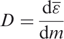
Absorbed dose, D

The absorbed dose is given by:

$D=\frac{\text{d}\overline{\varepsilon }}{\text{d}m}$

where d $\overline{\varepsilon }$ is the mean energy imparted by ionising radiation to matter of mass dm. The SI unit of absorbed dose is joule per kilogramme (J kg⁻¹), and its special name is gray (Gy).

Absorbed fraction, $\phi (r_{\text{T}}\to r_{\text{S}},E_{\text{R},\text{i}})$

Fraction of energy E_R,i of the i^th radiation of type R emitted within the source region r_S that is absorbed in the target region r_T. These target regions may be tissues (e.g. liver) or may be cell layers within organs (e.g. stem cells of the stomach wall) (see definitions for ‘Target region’ and ‘Target tissue’).

Active (bone) marrow

Active marrow is haematopoietically active and gets its red colour from the large numbers of erythrocytes (red blood cells) being produced. Active bone marrow serves as a target region for radiogenic risk of leukaemia.

Activity

The number of nuclear transformations of a radioactive material during an infinitesimal time interval, divided by its duration (s). The SI unit of activity is s⁻¹ and its special name is becquerel (Bq).

Biological half-life

The time required for a compartment of a biological system to eliminate (in the absence of additional input and radioactive decay) half of its radionuclide content.

Bone marrow [see also ‘Active (bone) marrow’ and ‘Inactive (bone) marrow’]

Bone marrow is a soft, highly cellular tissue that occupies the cylindrical cavities of long bones and the cavities defined by the bone trabeculae of the axial and appendicular skeleton. Total bone marrow consists of a sponge-like, reticular, connective tissue framework called ‘stroma’, myeloid (blood-cell-forming) tissue, fat cells (adipocytes), small accumulations of lymphatic tissue, and numerous blood vessels and sinusoids. There are two types of bone marrow: active (red) and inactive (yellow), where these adjectives refer to the marrow’s potential for the production of blood cell elements (haematopoiesis).

Committed effective dose, E(τ) (see also ‘Effective dose’)

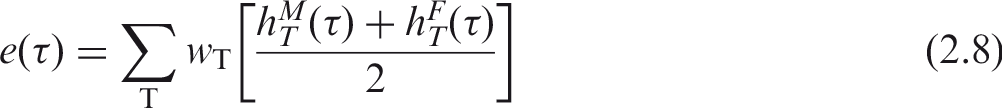
In the Occupational Intakes of Radionuclides publication series, the integration time τ following the intake is taken to be 50 years. The committed effective dose E(50) is calculated with the use of male and female committed equivalent doses to individual target organs or tissues, T, according to the expression:

$E(50)=\sum _T{w}_{\text{T}}[\frac{H_{\text{T}}^{\text{M}}(50)+H_{\text{T}}^{\text{F}}(50)}{2}].$

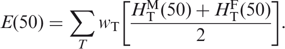
The SI unit for committed effective dose is the same as for absorbed dose, joule per kilogramme (J kg⁻¹), and its special name is sievert (Sv).

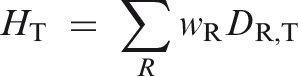
Committed equivalent dose, H_T (50) (see also ‘Equivalent dose’)

In the Occupational Intakes of Radionuclides publication series, the equivalent dose to an organ or tissue region is calculated using a 50-year commitment period. It is taken as the time integral of the equivalent dose rate in a target organ or tissue T of Reference Adult Male or Reference Adult Female. These, in turn, are predicted by reference biokinetic and dosimetric models following the intake of radioactive material into the body. The integration period is thus 50 years following the intake:

$H_{\text{T}}(50)={\int }_0^{50}\stackrel{·}{H}(r_{\text{T}},t)\mathrm{dt}.$

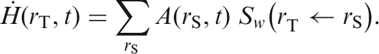
For both sexes, the equivalent dose rate 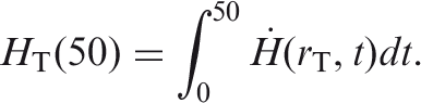$\stackrel{·}{H}(r_{\text{T}},t)$ in target region r_T at time t after an acute intake is expressed as:

$\stackrel{·}{H}(r_{\text{T}},t)=\sum _{r_{\text{S}}}A(r_{\text{S}},t)S_w(r_{\text{T}}\to r_{\text{S}}).$

where A(r_S, t) is the activity of the radionuclide in source region r_S at time t after intake, in Bq, as predicted by the reference biokinetic models for the Reference Adult; and S_w(r_T ← r_S) is the radiation-weighted S coefficient [i.e. the equivalent dose to target region r_T per nuclear transformation in source region r_S, in Sv (Bq s)⁻¹, for Reference Adult Male and Reference Adult Female].

The SI unit for committed equivalent dose is the same as for absorbed dose, joule per kilogramme (J kg⁻¹), and its special name is sievert (Sv).

Dose coefficient

For adults, a dose coefficient is defined as either the committed equivalent dose in tissue T per activity intake, h_T(50), or the committed effective dose per activity intake, e(50), where 50 is the dose-commitment period in years over which the dose is calculated. Note that elsewhere, the term ‘dose per intake coefficient’ is sometimes used for dose coefficient.

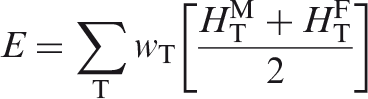
Effective dose, E

In accordance with the generic definition of effective dose in Publication 103 (ICRP, 2007), effective dose is calculated as:

$E=\sum _{\text{T}}{w}_{\text{T}}[\frac{H_{\text{T}}^{\text{M}}+H_{\text{T}}^{\text{F}}}{2}]$

where $H_{\text{T}}^{\text{M}}$ and $H_{\text{T}}^{\text{F}}$ are the equivalent doses to the tissues or organs r_T of Reference Adult Male and Reference Adult Female, respectively, and w_T is the tissue weighting factor for target tissue T, with $\sum _{\text{T}}{w}_{\text{T}}=1$ . The sum is performed over all organs and tissues of the human body considered to be sensitive to the induction of stochastic effects. As w_R and w_T are dimensionless, the SI unit for effective dose is the same as for absorbed dose, joule per kilogramme (J kg⁻¹), and its special name is sievert (Sv).

Endosteum (or endosteal layer)

A 50-μm-thick layer covering the surfaces of the bone in regions of trabecular spongiosa and surfaces of the medullary activities within the shafts of the long bones. It is assumed to be the target region for radiogenic bone cancer. The mass of the endosteum is 0.58 and 0.43 kg in the adult reference male and female, respectively. This target replaces the bone surface target of Publications 26 and 30 (1977, 1979, 1980, 1981, 1988), which was defined as a 10 μm layer of mass 0.12 kg.

Equivalent dose, H_T

The equivalent dose to a tissue or organ is defined as:

$H_{\text{T}}=\sum _R{w}_{\text{R}}{D}_{\text{R},\text{T}}$

where w_R is the radiation weighting factor for radiation type R, and D_R,T is the organ absorbed dose from radiation type R in a tissue or organ r_T of Reference Adult Male or Reference Adult Female. As w_R is dimensionless, the SI unit for the equivalent dose is the same as for absorbed dose, joule per kilogramme (J kg⁻¹), and its special name is sievert (Sv).

Gray (Gy)

The special name for the SI unit of absorbed dose.

Inactive (bone) marrow

In contrast to active marrow, inactive marrow is haematopoietically inactive (i.e. does not directly support haematopoiesis). It gets its yellow colour from fat cells (adipocytes) that occupy most of the space of the bone marrow framework.

Marrow cellularity

The fraction of bone marrow volume in a given bone that is haematopoietically active. Age- and bone-site-dependent reference values for marrow cellularity are given in Table 41 of Publication 70 (ICRP, 1995). As a first approximation, marrow cellularity may be thought of as one minus the fat fraction of bone marrow.

Mean absorbed dose, D_T

The mean absorbed dose in a specified target organ or tissue T is given by:

$D_{\text{T}}=1/m_{\text{T}}\int \mathrm{Ddm}$

where m_T is the mass of the organ or tissue, and D is the absorbed dose in the mass element dm. The SI unit of mean absorbed dose is joule per kilogramme (J kg⁻¹), and its special name is gray (Gy).

Other tissues

A term used in biokinetic models to represent in a collective manner tissues not identified explicitly in the biokinetic model.

Radiation weighting factor, w_R

A dimensionless factor by which the organ or tissue absorbed dose component of radiation type R is multiplied to reflect the relative biological effectiveness of that radiation type. It is used to derive the organ equivalent dose from the mean absorbed dose in an organ or tissue.

Red (bone) marrow

See ‘Active (bone) marrow’.

Reference Male and Reference Female

Reference males and females are defined as either adults or children of ages 0, 1, 5, 10, and 15 years.

Reference parameter value

The value of a parameter, factor, or quantity that is regarded as valid for use in dosimetric calculations and recommended by ICRP. These values are fixed and are not subject to uncertainties.

Reference Person

An idealised person for whom the equivalent doses to organs and tissues are calculated by averaging the corresponding organ doses in the Reference Male and Reference Female. The equivalent doses of Reference Person are used for the calculation of effective dose.

Reference phantom

The computational phantom of the human body (male or female voxel phantom based on medical imaging data), defined in Publication 110 (ICRP, 2009), with the anatomical and physiological characteristics of Reference Male and Reference Female defined in Publication 89 (ICRP, 2002).

Sievert (Sv)

The special name for the SI unit (J kg⁻¹) of equivalent dose and effective dose.

Source region, r_S

Region of the body containing the radionuclide. The region may be an organ, a tissue, the contents of the alimentary tract or urinary bladder, or the surfaces of tissues, such as in the skeleton and the respiratory tract.

Specific absorbed fraction (SAF), $\Phi (r_{\text{T}}\to r_{\text{S}},E_{\text{R},\text{i}})$

Fraction of radiation R of energy E_R,i emitted within the source region r_S that is absorbed per mass in the target region r_T.

Spongiosa

Term referring to the combined tissues of the bone trabeculae and marrow tissues (both active and inactive) located beneath cortical bone cortices across regions of the axial and appendicular skeleton. Spongiosa is one of three bone regions defined in the Publication 110 (ICRP, 2009) reference phantoms, the other two being cortical bone and medullary marrow of the long bone shafts. As the relative proportions of trabecular bone, active marrow, and inactive marrow vary with skeletal site, the homogeneous elemental composition and mass density of spongiosa are not constant but vary with skeletal site (see Annex B of Publication 110).

S coefficient (radiation-weighted), $S_w(r_{\text{T}}\to r_{\text{S}})$

The equivalent dose to target region r_T per nuclear transformation of a given radionuclide in source region r_S, Sv (Bq s)⁻¹, for Reference Adult Male and Reference Adult Female.

$S_w(r_{\text{T}}\to r_{\text{S}})=\sum _R{w}_{\text{R}}\sum _i{E}_{\text{R},\text{i}}{Y}_{\text{R},\text{i}}\Phi (r_{\text{T}}\to r_{\text{S}},E_{\text{R},\text{i}})$

$\text{where}\hspace{1em}{E}_{R,i}$ is the energy of the i^th radiation of type R emitted in nuclear transformations of the radionuclide (J); $Y_{\text{R},\text{i}}$ is the yield of the i^th radiation of type R per nuclear transformation [(Bq s)⁻¹]; $w_{\text{R}}$ is the radiation weighting factor for radiation type R (Table 2.1); and $\Phi (r_{\text{T}}\to r_{\text{S}},E_{\text{R},\text{i}})$ is the specific absorbed fraction, defined as the fraction of energy $E_{\text{R},\text{i}}$ of radiation type R emitted within the source region r_S that is absorbed per mass in the target region r_T (kg⁻¹).

Table 2.1.

International Commission on Radiological Protection radiation weighting factors.

Radiation type	Radiation weighting factor, wR
Photons	1
Electrons and muons	1
Protons and charged pions	2
Alpha particles, fission fragments, heavy ions	20
Neutrons	Continuous function of neutron energy See Eq. (4.3) of Publication 103*

*

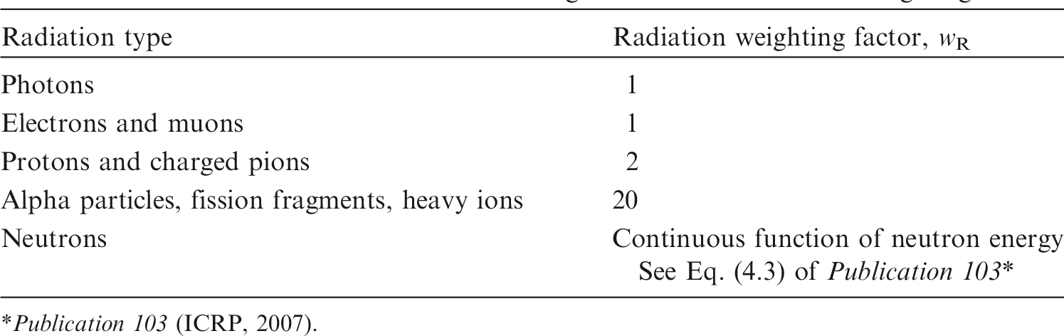
Publication 103 (ICRP, 2007).

In adults, no change in anatomical parameters are considered with time (age). Thus S_w is invariant in time and its numerical value represents either the equivalent dose rate in the target tissue (Sv s⁻¹) per activity (Bq) in the source region or the equivalent dose (Sv) per nuclear transformation (Bq s).

Target region, r_T

A tissue region of the body in which a radiation absorbed dose or equivalent dose is received.

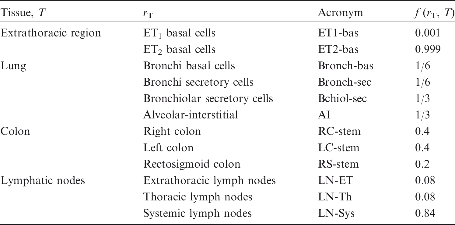
Target tissue, T

Organ or tissue in the body for which tissue weighting factors are assigned in the effective dose (Table 2.2). In many cases, each target tissue T corresponds to a single target region r_T. In the case of the extrathoracic region, lungs, colon, and lymphatic nodes, however, a fractional weighting of more than one target region r_T defines the target tissue T (Table 2.3).

Table 2.2.

International Commission on Radiological Protection tissue weighting factors.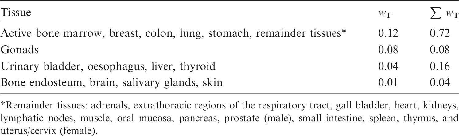

Tissue	w T	∑ wT
Active bone marrow, breast, colon, lung, stomach, remainder tissues*	0.12	0.72
Gonads	0.08	0.08
Urinary bladder, oesophagus, liver, thyroid	0.04	0.16
Bone endosteum, brain, salivary glands, skin	0.01	0.04

*

Remainder tissues: adrenals, extrathoracic regions of the respiratory tract, gall bladder, heart, kidneys, lymphatic nodes, muscle, oral mucosa, pancreas, prostate (male), small intestine, spleen, thymus, and uterus/cervix (female).

Table 2.3.

Target region fractional weights, f (r_T, T).

Tissue, T	r T	Acronym	f (rT, T)
Extrathoracic region	ET1 basal cells	ET1-bas	0.001
	ET2 basal cells	ET2-bas	0.999
Lung	Bronchi basal cells	Bronch-bas	1/6
	Bronchi secretory cells	Bronch-sec	1/6
	Bronchiolar secretory cells	Bchiol-sec	1/3
	Alveolar-interstitial	AI	1/3
Colon	Right colon	RC-stem	0.4
	Left colon	LC-stem	0.4
	Rectosigmoid colon	RS-stem	0.2
Lymphatic nodes	Extrathoracic lymph nodes	LN-ET	0.08
	Thoracic lymph nodes	LN-Th	0.08
	Systemic lymph nodes	LN-Sys	0.84

Tissue weighting factor, w_T (see also ‘Effective dose’)

The factor by which the equivalent dose to an organ or tissue r_T is weighted to represent the relative contribution of that organ or tissue to overall radiation detriment from stochastic effects (see Publication 103 (ICRP, 2007)).

1. Introduction

(1) The system of radiological protection recommended by the International Commission on Radiological Protection (ICRP) is the basis for standards and working practices throughout the world (ICRP, 1991, 2007; IAEA, 2014). Fundamental to the application of ICRP recommendations are the protection quantities defined by ICRP: equivalent dose and effective dose. While the definition of these quantities remains unchanged in the most recent recommendations (ICRP, 2007), there have been important changes that affect the values calculated per radiation exposure. ICRP Committee 2 is responsible for the provision of these reference dose coefficients for the assessment of internal radiation exposure, calculated using reference biokinetic and dosimetric models, and reference data for adults and other members of the public. Following the 2007 Recommendations (ICRP, 2007), Committee 2 and its task groups engaged in a substantial programme of work to provide new dose coefficients for various circumstances of radiation exposure.

(2) The underlying foundations of radionuclide dose coefficients for internal exposures include several reference parameters and models. These include, among others: (i) masses of organs and tissues in Reference Adult Male and Reference Adult Female; (ii) radionuclide decay information; (iii) biokinetic models for inhalation, ingestion, and systemic biodistribution; and (iv) specific absorbed fraction (SAF) values. Publications 89 and 107 (ICRP, 2002, 2008) provide reference organ masses and radionuclide decay data, respectively, as needed for calculations of internal dose coefficients. Publications 66 and 100 (ICRP, 1994a, 2006) provide models for inhalation and ingestion of radionuclides, respectively. Presently, the ICRP Task Group on Internal Dose Coefficients is completing an extensive set of revisions to its systemic biokinetic models within its Occupational Intakes of Radionuclides (OIR) publication series. The purpose of this publication, prepared by the ICRP Task Group on Computational Phantoms and Radiation Transport, is to document the development and provide data for SAFs for a wide range of internally emitted radiations (photons, electrons, alpha particles, and – in the case of radionuclides undergoing spontaneous fission – neutrons) for all relevant combinations of source and target tissues. The SAF is defined as the fraction of radiation energy emitted within a source region that is absorbed per mass in a target region. These tissue regions can be whole organs, organ subregions, individual cell layers, or tissue interface surfaces. The values given in this publication are for Reference Adult Male and Reference Adult Female, as defined in Publication 103 (ICRP, 2007), and are used within the OIR publication series in the calculation of ICRP reference dose coefficients for inhalation and ingestion. Further information is given in OIR Part 1 (ICRP, 2015).

2. ICRP Schema for Internal Dose Assessment

(3) The ICRP dosimetry schema is presented below as applied to assessment of tissue-specific equivalent dose and effective dose following intakes of radionuclides. The system involves numerical solution of reference biokinetic models, yielding the time-dependent number of nuclear transformations in various source regions. These solutions are then coupled with reference data on nuclear decay information, target tissue masses, and fractions of emitted energy released from source regions that are deposited in target regions as defined in the Publication 110 reference phantoms (ICRP, 2009). Presented below is the computational formalism of these dosimetry calculations consistent with the protection quantities defined in Publication 103 (ICRP, 2007).

(4) As defined in Publication 103 (ICRP, 2007) (and the Glossary of the present publication), the effective dose employs two forms of weighting factors. The first is the radiation weighting factor, w_R, used in the calculation of the tissue equivalent dose given computed values of tissue absorbed dose. Values of w_R are shown in Table 2.1. The second is the tissue weighting factor, w_T, used in the calculation of the effective dose given computed values of sex-averaged organ equivalent doses. Values of w_T are shown in Table 2.2.

2.1. Computational solutions to the ICRP reference biokinetic models

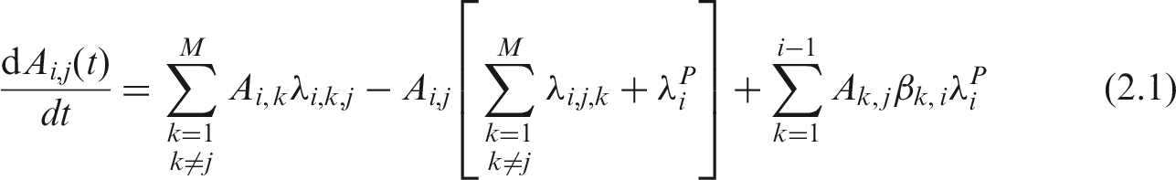
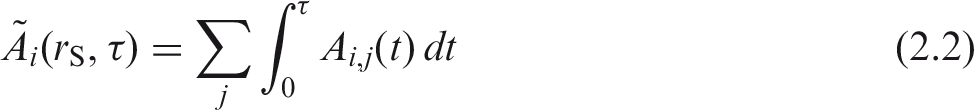
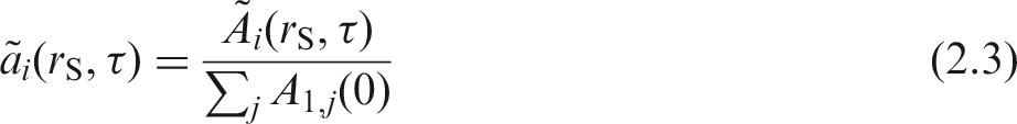
(5) The Human Respiratory Tract Model (HRTM) (ICRP, 1994a), the Human Alimentary Tract Model (HATM) (ICRP, 2006), and the systemic biokinetic models of the OIR publication series describe the dynamic behaviour of radionuclides within the body. Given the routes of intake, the models predict subsequent uptake to the systemic circulation, distribution among tissues of the body, and routes of elimination from the body. Superimposed on these dynamics are in-situ radioactive decay and ingrowth of radioactive progeny. Consequently, uptake, distribution, and elimination of all decay products are predicted, in addition to those of the parent radionuclide.

(6) The compartment models of the respiratory and alimentary tract coupled with those of the systemic biokinetics define a system of first-order differential equations. The solution to the set of equations is the time-dependent distribution of the radionuclide and its radioactive progeny, if any, in mathematical compartments (pools) that are associated with anatomical regions in the body. Let $A_{i,j}$ (t) represent the activity of radionuclide i in compartment j at time t. The rate of change in the activity of member i of the decay chain, i = 1, 2, … , N with i = 1 being the parent nuclide, in compartment j, can be written as:

$\frac{\text{d}{A}_{i,j}(t)}{\mathrm{dt}}=\sum _{\genfrac{}{}{0ex}{}{k=1}{k\ne j}}^M{A}_{i,k}{\lambda }_{i,k,j}-A_{i,j}[\sum _{\genfrac{}{}{0ex}{}{k=1}{k\ne j}}^M{\lambda }_{i,j,k}+{\lambda }_i^P]+\sum _{k=1}^{i-1}{A}_{k,j}{\beta }_{k,i}{\lambda }_i^P$

(2.1)

where: M

is the number of compartments describing the kinetics;

${\lambda }_{i,j,k}$

is the fractional transfer rate of chain member i from compartment j (donor compartment) to compartment k (receiving compartment) in the biokinetic model;

${\lambda }_i^P$

is the physical decay constant of chain member i; and

${\beta }_{k,i}$

is the fraction of the decays of chain member k forming member i.

(7) Given the initial conditions specified for the compartments, $A_{i,j}$ (0), Eq. (2.1) defines the dynamic behaviour of the radionuclide and its progeny within the human body. The first term on the right-hand side of Eq. (2.1) represents the rate of flow of chain member i into compartment j from all donor compartments. The second term represents the rate of removal of member i from compartment j, both by transfer to receiving compartments and by physical decay. The third term addresses the ingrowth of member i within compartment j due to the presence of its precursors k in the compartment. Note that the members of the decay chain are assumed to be of the order such that the precursors of member i have indices less than i. An ordered listing of the chain members can be obtained using the DECDATA software distributed with Publication 107 (ICRP, 2008).

(8) The system of N × M ordinary first-order differential equations must be solved using suitable numerical methods. The system is generally solved for the initial conditions that $A_{i,j}(0)=0$ for all compartments, with the exception of compartments of intake where non-zero initial conditions are only applied to the parent nuclide (i.e. $i=1$ ). In the case of inhalation of radon and its progeny, non-zero initial conditions may be assigned to progeny within the compartments of the respiratory tract (i.e. inhalation of short-lived radon progeny in the inspired air).

(9) To calculate the numerical values of the dose coefficients, it is necessary to associate the biokinetic compartments of Eq. (2.1) with anatomical regions in the body; so-called source regions indexed by $r_{\text{S}}$ . The source regions may or may not be a living tissue; for example, the contents of the alimentary tract are not a living tissue, and may consist of more than one kinetic compartment. The number of nuclear transformations of chain member i occurring in source region $r_{\text{S}}$ , ${\tilde{A}}_i(r_{\text{S}},\tau )$ (Bq s), is given by:

${\tilde{A}}_i(r_{\text{S}},\tau )=\sum _j{\int }_0^{\tau }{A}_{i,j}(t)\mathrm{dt}$

(2.2)

where τ is the commitment period (taken to be 50 years for adults). The summation in Eq. (2.2) is over all kinetic compartments j associated with source region $r_{\text{S}},$ and the quantity $A_{i,j}(t)$ is obtained by solving Eq. (2.1). The number of nuclear transformations per activity intake in the source region $r_{\text{S}}$ , denoted as ${\tilde{a}}_i(r_{\text{S}},\tau )$ (s), is given by:

${\tilde{a}}_i(r_{\text{S}},\tau )=\frac{{\tilde{A}}_i(r_{\text{S}},\tau )}{\sum _j{A}_{1,j}(0)}$

(2.3)

where the summation in the denominator is over the compartment contents at t = 0. In the case of inhalation of particulate and gaseous matter, the denominator includes the exhaled activity as only a fraction of the activity intake is deposited in the compartments of the HRTM.

2.2. Computation of ICRP reference dose coefficients for equivalent dose

(10) The committed equivalent dose coefficient in target region $r_{\text{T}}$ of Reference Adult Male, $hM(r_{\text{T}},\tau )$ and Reference Adult Female, $hF(r_{\text{T}},\tau )$ for integration time τ is given by:

$$hM(r_{\text{T}},\tau )=\sum _i\sum _{r_{\text{S}}}{\tilde{a}}_i(r_{\text{S}},\tau )S_w^M(r_{\text{T}}\to r_{\text{S}}{)}_i$$

(2.4)

$$hF(r_{\text{T}},\tau )=\sum _i\sum _{r_{\text{S}}}{\tilde{a}}_i(r_{\text{S}},\tau )S_w^F(r_{\text{T}}\to r_{\text{S}}{)}_i$$

(2.5)

where the S coefficients, $S_w^M(r_{\text{T}}\to r_{\text{S}}{)}_i$ and $S_w^F(r_{\text{T}}\to r_{\text{S}}{)}_i$ , are the radiation-weighted equivalent doses in target region $r_{\text{T}}$ per nuclear transformation of chain member i in source region $r_{\text{S}}$ [Sv (Bq s)⁻¹] for the male and female adult, respectively. Note that the outer summation extends over the parent nuclide and its progeny.

(11) A number of tissues listed in Table 2.2 used to compute the effective dose are considered to be represented by a single target region $r_{\text{T}}$ . In cases where more than one tissue region defines the target tissue, fractional weighting of the equivalent dose must be made. The committed equivalent dose coefficients for tissue T in Reference Adult Male, $h_T^M(\tau )$ , and Reference Adult Female, $h_T^F(\tau )$ , are thus given as:

$$h_T^M(\tau )=\sum _{r_{\text{T}}}f(r_{\text{T}},T)hM(r_{\text{T}},\tau )$$

(2.6)

$$h_T^F(\tau )=\sum _{r_{\text{T}}}f(r_{\text{T}},T)hF(r_{\text{T}},\tau )$$

(2.7)

where the target region fractional weights $f(r_{\text{T}},T)$ are the proportions of the equivalent dose in tissue T associated with target region $r_{\text{T}}$ . With the exception of the tissues addressed in Table 2.3, the tissues of Table 2.2 are represented by a single target region, and thus for these tissues $f(r_{\text{T}},T)=1.$ In Table 2.3, the $f(r_{\text{T}},T)$ values for the extrathoracic and thoracic (lung) regions are taken to be equivalent to their risk apportionment factors as assigned in the revised HRTM. For the colon, $f(r_{\text{T}},T)$ values are taken to be the rounded fractional masses of the stem cell layers within the alimentary tract walls in Publication 100 (ICRP, 2006). For the lymphatic nodes, $f(r_{\text{T}},T)$ values are taken to be the fractional masses of lymphatic nodes (not lymphatic tissues) within the extrathoracic, thoracic, and non-respiratory regions, consistent with data given in Publication 66 (ICRP, 1994).

2.3. Computation of ICRP reference dose coefficients for effective dose

(12) As defined in Publication 103 (ICRP, 2007), the committed effective dose coefficient, $e(\tau )$ , is:

$e(\tau )=\sum _{\text{T}}{w}_{\text{T}}[\frac{h_T^M(\tau )+h_T^F(\tau )}{2}]$

(2.8)

where w_T is the tissue weighting factor for target tissue T, and $h_T^M(\tau )$ and $h_T^F(\tau )$ are the corresponding committed equivalent dose coefficients for these same tissues in Reference Adult Male and Reference Adult Female, respectively.

2.4. Implementation of specific absorbed fractions within the ICRP system

(13) The radiation-weighted S coefficient for a radionuclide is calculated as:

$S_w(r_{\text{T}}\to r_{\text{S}})=\sum _R{w}_{\text{R}}\sum _i{E}_{\text{R},\text{i}}{Y}_{\text{R},\text{i}}\Phi (r_{\text{T}}\to r_{\text{S}},E_{\text{R},\text{i}})$

(2.9)

where $E_{\text{R},\text{i}}$ is the energy of the i^th radiation of type R emitted in nuclear transformations of the radionuclide (J); $Y_{\text{R},\text{i}}$ is the yield of the i^th radiation of type R per nuclear transformation [(Bq s)⁻¹]; $w_{\text{R}}$ is the radiation weighting factor for radiation type R (Table 2.1); and $\Phi (r_{\text{T}}\to r_{\text{S}},E_{\text{R},\text{i}})$ is the SAF, defined as the fraction of energy $E_{\text{R},\text{i}}$ of radiation type R emitted within the source tissue r_S that is absorbed per mass in the target tissue r_T (kg⁻¹).

(14) The energies and yields of the emitted radiations, $E_{R,i}$ and $Y_{R,i}$ , are taken from Publication 107 (ICRP, 2008). For beta emissions, the spectral data are used in the calculation of S_w rather than mean values [i.e. the inner summation in Eq. (2.9) is replaced by the integral over the beta-particle spectrum].

(15) SAF values given in this publication are calculated as the quotient of the absorbed fraction and the target tissue mass. Values of the absorbed fraction are calculated by radiation transport simulation using either voxelised or stylised (mathematically defined) geometries as outlined further in Sections 3–6. Values of reference target tissue masses used in SAF calculations are listed in Tables A.1 and A.2 of Annex A. For tissues containing blood, the computed energy absorption takes place over the entire volume of the tissue; therefore, it is necessary to divide the absorbed fraction by a target tissue mass inclusive of blood. Tables A.1 and A.2 detail how the blood mass is added to each target tissue. When considering the mass of source regions, however, it is generally desirable to consider the parenchyma mass alone, exclusive of blood, as blood is a separate source region considered explicitly in the latest biokinetic models. Table A.3 contains the source region definitions and their associated masses for both the Reference Adult Male and Reference Adult Female.

2.5. Derivation of specific absorbed fractions for distributed source organs

(16) Systemic biokinetic models indicate radionuclide deposition from blood to various identified source regions r_S, each with its own compartmental representation in the biokinetic model. In many instances, the balance of radionuclide deposition from blood will be assigned to ‘other tissues’ of the body, which implies all other soft tissues not explicitly identified as source organs. To address this source region, which is generally unique to a given radionuclide biokinetic model, one must derive the SAF for the relevant target tissue r_T. This SAF is calculated using the so-called additive approach as:

$\Phi (r_{\text{T}}\to \mathrm{Other})=\frac{1}{M_{\mathrm{Other}}}\sum _{r_{\text{S}}}{M}_{r_{\text{S}}}\Phi (r_{\text{T}}\to r_{\text{S}})$

(2.10)

where the summation is over source regions not included explicitly in the systemic biokinetic model. Unless noted specifically in the biokinetic model, deposition to other tissues is not assigned to mineral bone in either its cortical or trabecular form. A summary of reference source tissue masses is given in Table A.3.

3. Computational Methods for whole-body organs

3.1. The ICRP/ICRU reference computational phantoms

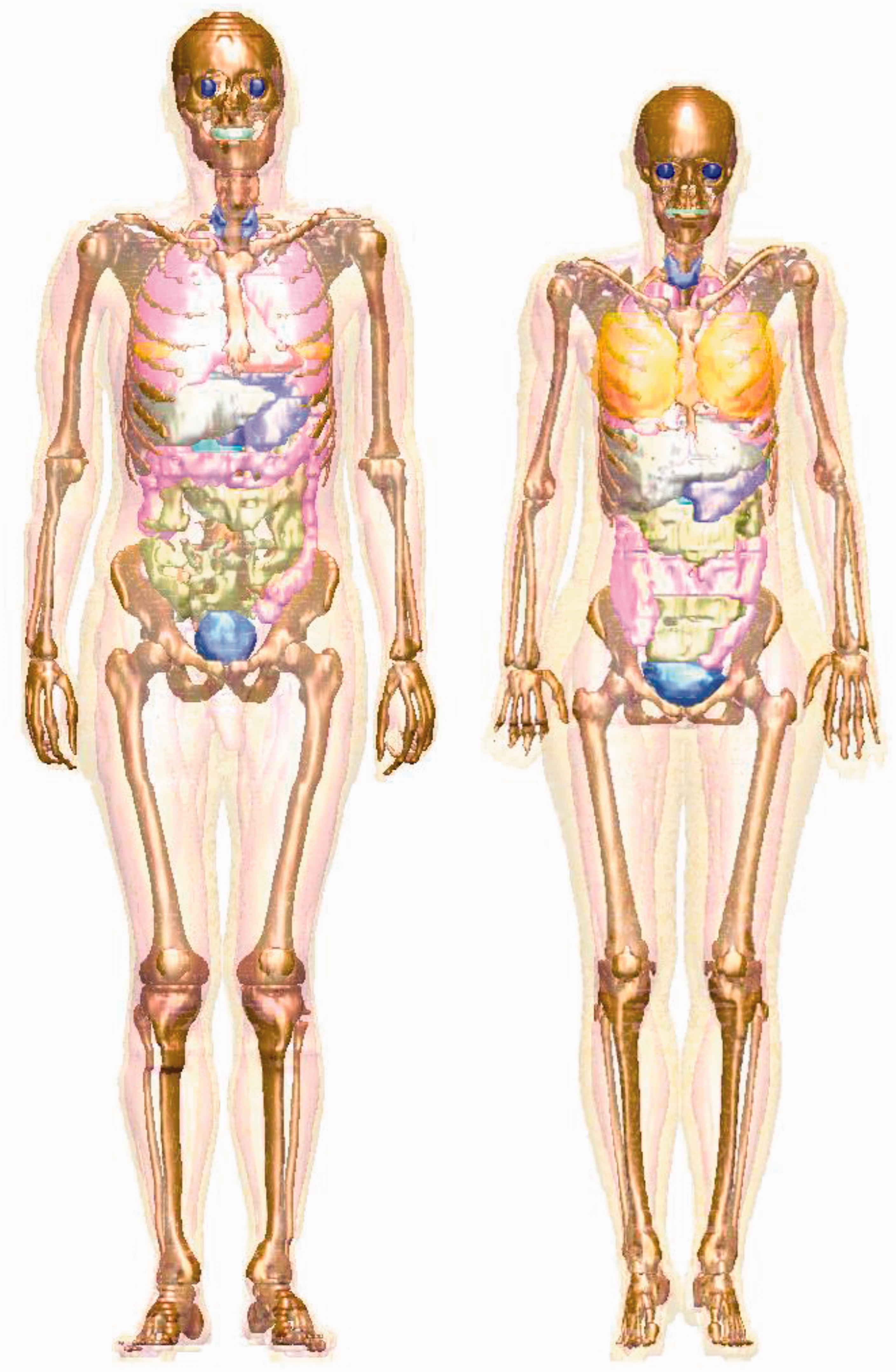
(17) The adult male and female reference computational phantoms, representing Reference Male and Reference Female (ICRP, 2007), were used in this publication for the computation of organ absorbed doses. These phantoms were adopted by ICRP and the International Commission on Radiation Units and Measurements (ICRU) as the phantoms for computation of the ICRP reference dose coefficients, and are described extensively in Publication 110 (ICRP, 2009). The reference computational phantoms are digital three-dimensional (3D) representations of human anatomy, and are based on human computed tomographic (CT) data. They are consistent with the information given in Publication 89 (ICRP, 2002) on the reference anatomical parameters for both male and female adults. The reference computational phantoms (or models) were constructed by modifying the voxel models (Zankl and Wittmann, 2001; Zankl et al., 2005) of two individuals (Golem and Laura) whose body height and mass closely resembled the reference data. The organ masses of both phantoms were adjusted to the ICRP data on Reference Male and Reference Female with high precision, without significantly altering their realistic anatomy. The phantoms contain all target regions relevant to the assessment of human exposure to ionising radiation for radiological protection purposes, i.e. all organs and tissues that contribute to effective dose (ICRP, 2007).

(18) Each phantom is represented in the form of a 3D array of cuboid voxels. Each voxel is a volume element, and the voxels are arranged in columns, rows, and slices. Each voxel in the array identifies the organ or tissue to which it represents. The male reference computational phantom consists of approximately 1.95 million tissue voxels (excluding voxels representing the surrounding vacuum), each with a slice thickness (corresponding to voxel height) of 8.0 mm and an in-plane resolution (i.e. voxel width and depth) of 2.137 mm, corresponding to a voxel volume of 36.54 mm³. The number of slices is 220, resulting in a body height of 1.76 m; the body mass is 73 kg. The female reference computational phantom consists of approximately 3.89 million tissue voxels, each with a slice thickness of 4.84 mm and an in-plane resolution of 1.775 mm, corresponding to a voxel volume of 15.25 mm³. The number of slices is 346, and the body height is 1.63 m; the body mass is 60 kg. The number of individually segmented structures is 136 in each phantom, and 53 different tissue compositions have been assigned. The various tissue compositions reflect both the elemental composition of the tissue parenchyma (ICRU, 1992) and each organ’s blood content (ICRP, 2002) (i.e. organ composition inclusive of blood). Fig. 3.1 shows frontal (coronal) views of the male (left) and female (right) computational phantoms.

(19) Due to the limited resolution of the tomographic data on which these phantoms are based, and the very small dimensions of some of the source and target regions, not all tissues could be represented explicitly. In the skeleton, for example, the target tissues of interest are the red bone marrow in the marrow cavities of spongiosa, and the endosteal layer lining these cavities (presently assumed to be 50 µm in thickness). Due to their small dimensions, these two target tissues had to be incorporated as homogeneous constituents of spongiosa within the reference phantoms. At lower energies of photons and neutrons, secondary charged-particle equilibrium is not fully established in these tissue regions over certain energy ranges. More refined techniques for accounting for these effects in skeletal dosimetry are discussed in Section 4.

(20) Similarly, the fine structure of some of the target regions in the human respiratory tract and human alimentary tract could not be described by the voxel geometry of the reference phantoms, and thus stylised models of the airways and of individual segments of the alimentary tract were employed for electrons and alpha particles in the respiratory and alimentary tracts. However, for photon SAFs and for electron cross-irradiation SAFs from and to source and target regions outside the human respiratory tract and human alimentary tract, the representations of these two organ systems, as described in the reference computational phantoms, were used.

(21) Small to moderate differences exist in the masses of the target tissues in the computational phantom [given in Annex A of Publication 110 (ICRP, 2009)] and the masses given in Tables A.1 (male) and A.2 (female) of this publication, as the latter includes the blood content of the target tissue. For cross-fire geometries, Petoussi-Henss et al. (2007) demonstrated the principle given in MIRD Pamphlet No. 5, Revised (Snyder et al., 1978) and MIRD Pamphlet No. 11 (Snyder et al., 1975) that the SAF is independent of target mass. Consequently, all cross-fire SAFs were calculated with the computational phantoms (Zankl et al., 2012), according to the specifications of the source and target regions as given in Annex C (source regions) and Annex D (target regions) of Publication 110 (ICRP, 2009). A summary of source tissue masses is correspondingly given in Table A.3 of this publication.

(22) Self-irradiation SAFs for all radiation types were calculated by taking the self-irradiation absorbed fractions from the computational phantoms and dividing by the target mass given in Tables A.1 and A.2 of this publication. For self-irradiation geometries, Snyder (1970) described the photon absorbed fraction varying in proportion to the cube root of the target mass. This proportionality holds for photon energies and media where Compton scattering is the dominant interaction. As the differences in the computational phantom organ mass and the reference target mass are small, simply dividing the derived absorbed fraction by the reference target mass results in minor absolute differences in the SAF while allowing for an improved SAF at low photon energies.

(23) The blood source is an exception to the above cross-fire discussion, as the blood content of the target contributed significantly to the energy deposition in the target tissue. Thus, target tissue SAFs for the blood source for all radiations were calculated by taking the cross-fire irradiation absorbed fractions and dividing by the target mass given in Tables A.1 and A.2 of this publication.

(24) This discussion does not apply to epithelial targets for the HATM and HRTM as they are specified in terms of a tissue layer at depth.

Fig. 3.1.

Images of the adult male (left) and adult female (right) computational phantoms. The following organs can be identified by different surface colours: breast, bones, colon, eyes, lungs, liver, pancreas, small intestine, stomach, teeth, thyroid, and urinary bladder. Muscle and adipose tissue are semi-transparent. For illustration purposes, the voxelised surfaces have been smoothed.

3.2. Radiation transport codes used for absorbed fraction calculations

3.2.1. Photon and electron transport calculations

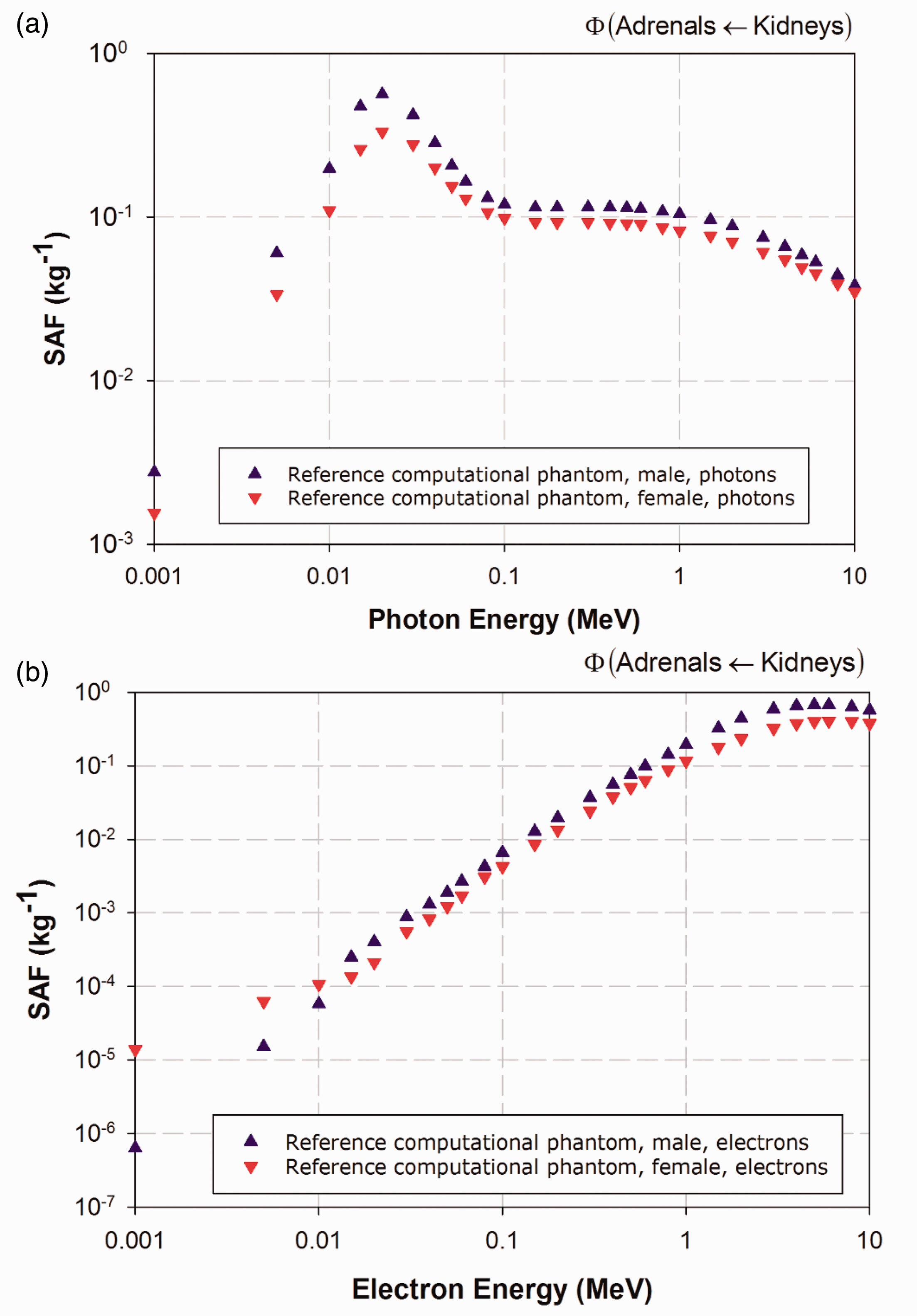
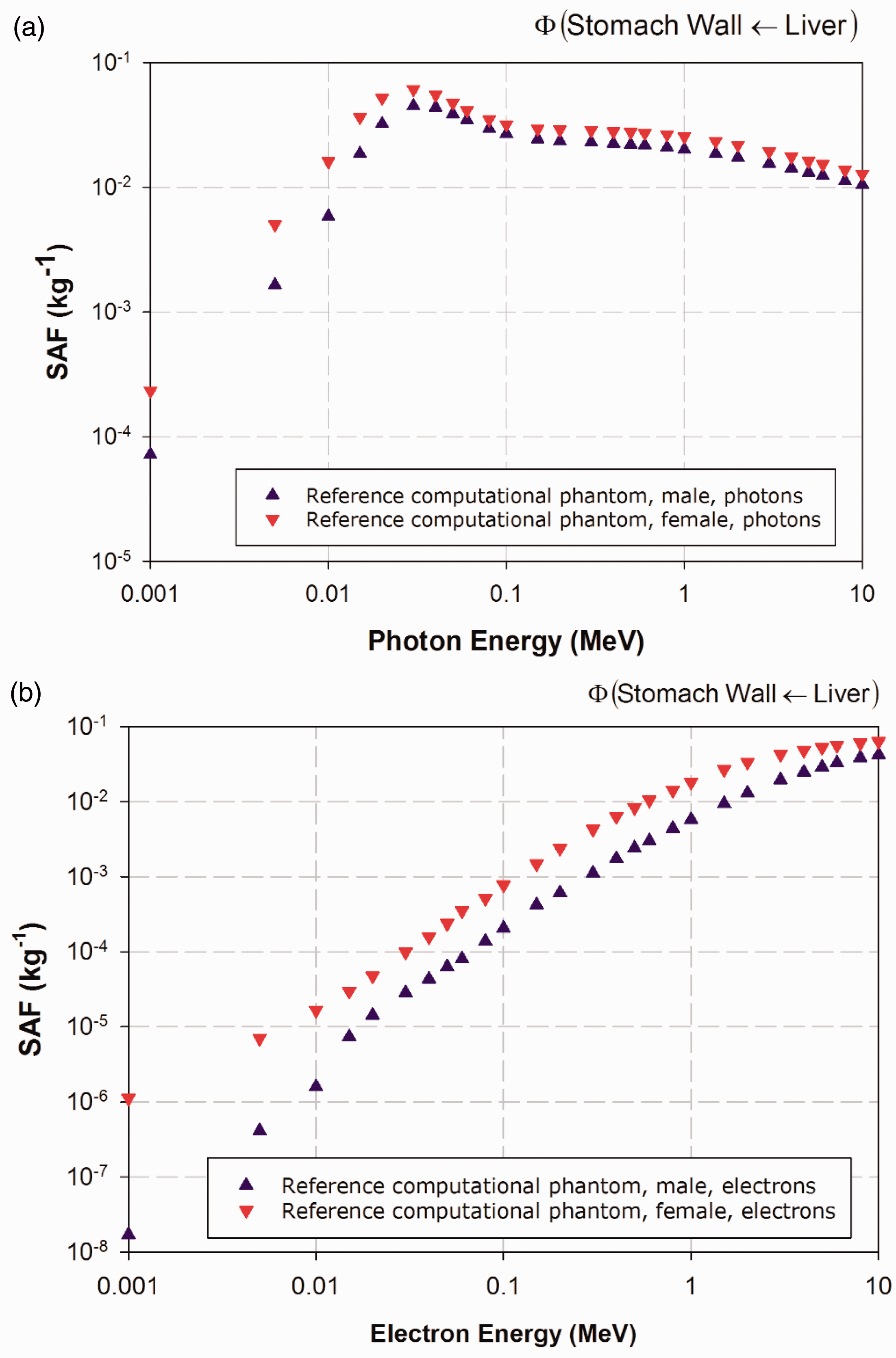
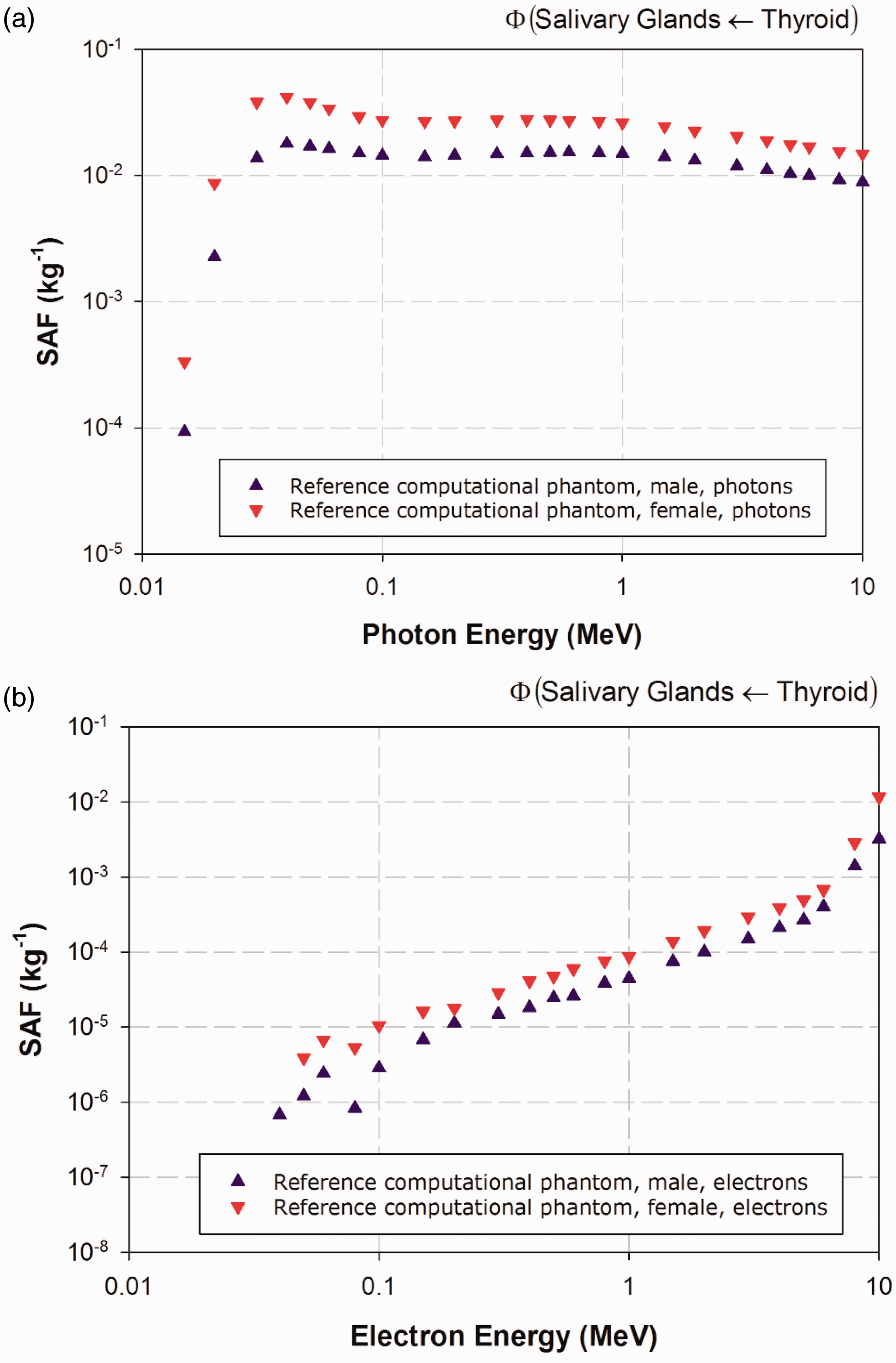
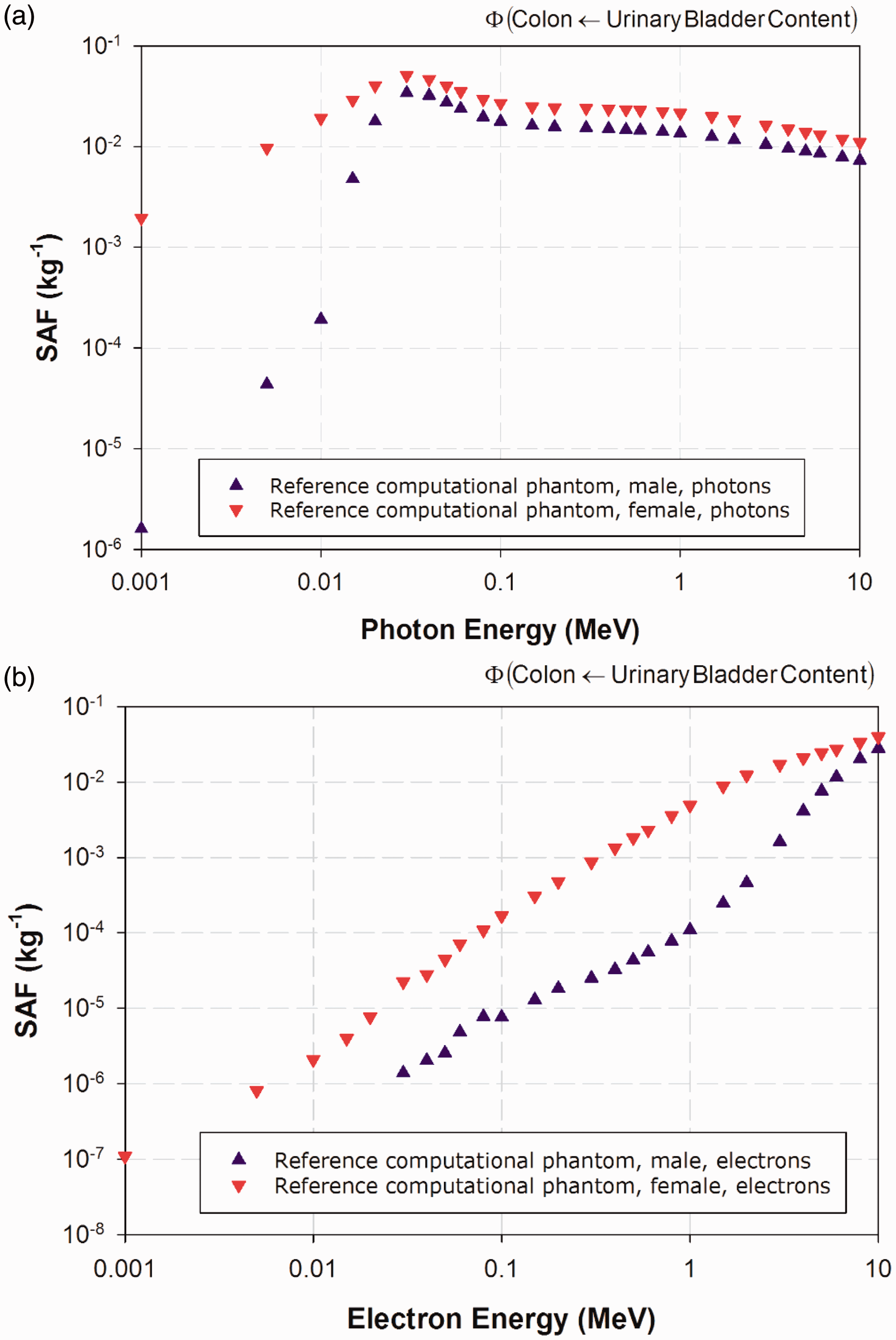
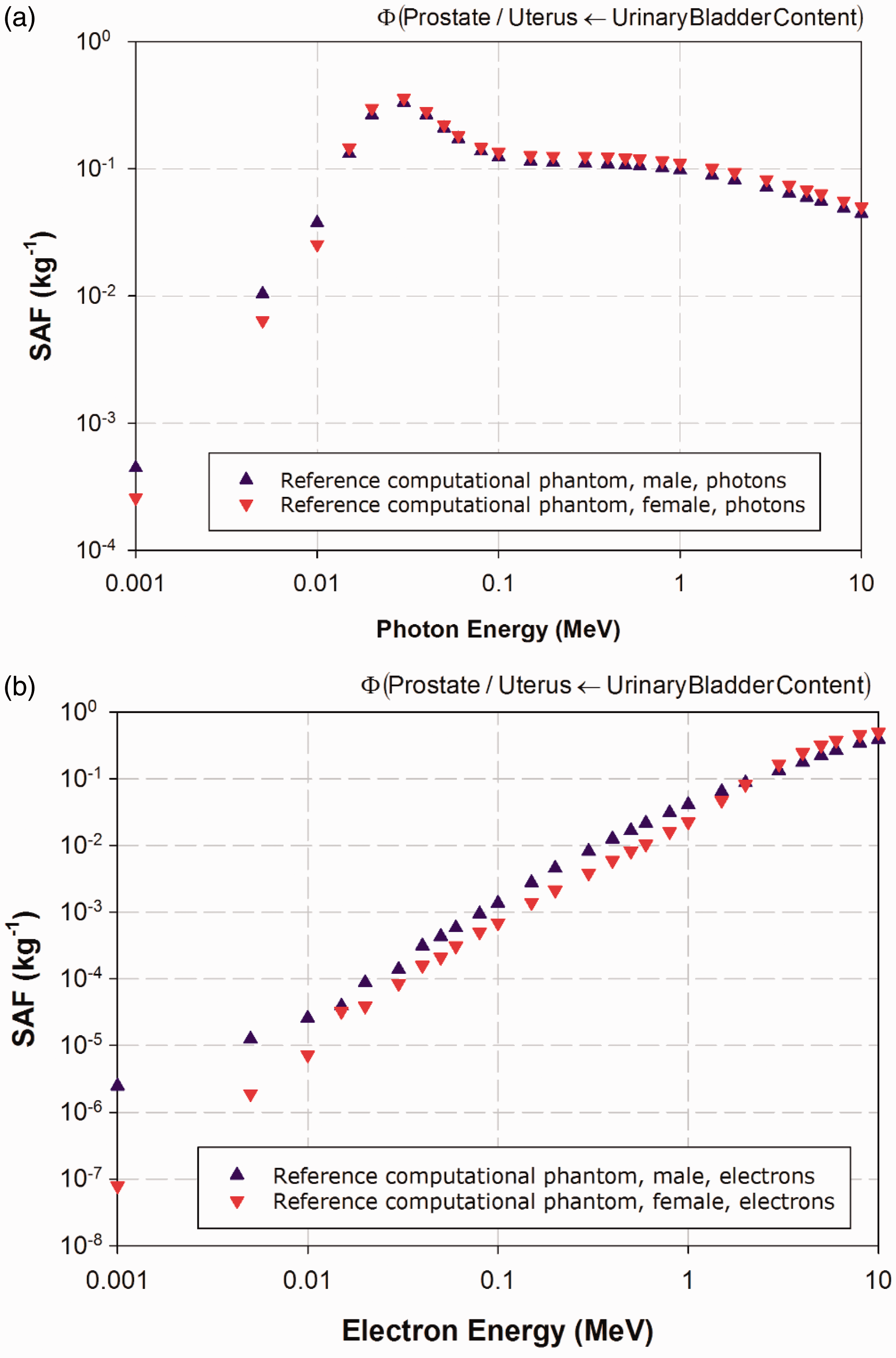
(25) The electron-gamma-shower code system EGSnrc Version v4-2-3-0 has been used for calculations of photon and electron absorbed fractions in this publication for reporting corresponding SAFs (Kawrakow et al., 2009). This code is an extended and improved version of EGS4 (Nelson et al., 1985), maintained by the National Research Council of Canada. The transport of photons and electrons can be simulated for particle kinetic energies from a few keV up to several hundred GeV, although simulations performed in this study were made over the energy range of 10 keV to 10 MeV. Values of SAF below 10 keV were determined via interpolation to limiting values, as described in Annex B.

(26) For photon transport, bound Compton scattering and photo-electrons from K, L, and M shells are considered for all energies. In all cases, resulting fluorescence or Auger and Coster-Kronig electrons are followed. The input data for photon cross-sections have been updated by Seuntjens et al. (2002), who used the XCOM database (Berger and Hubbell, 1987) to improve the cross-sections for the photo-electric effect, Rayleigh scattering, and pair production. Radiative Compton corrections in the one-loop approximation based on the Brown and Feynman equation (1952) are applied. However, the effect of reducing the cross-section for large scattering angles is partially cancelled by the inclusion of double-Compton events. For the pair-production cross-section, cross-sections in EGS4 are employed following the techniques of Øverbø et al. (1973). In this publication, photon transport is terminated when the photon energy falls below 2 keV.

(27) Electron transport calculations are performed by a Class II condensed history technique (Berger, 1963), which transports secondary particles produced above a certain chosen energy. Bremsstrahlung cross-sections agree with those of the National Institute of Standards and Technology database (Seltzer and Berger, 1985, 1986), which in turn form the basis for the radiative stopping powers recommended by ICRU (1984). Electron impact ionisation is modelled using default cross-sections (Kawrakow, 2002). For elastic scattering, spin effects are taken into account. Pair production is simulated as in EGS4 (Nelson et al., 1985). Triplet-production processes are neglected for all particles. In this publication, the transport history of electrons is generally terminated when their kinetic energy falls below 20 keV. Exceptions are noted for electrons with an initial kinetic energy below 50 keV, whose histories are followed down to 2 keV. A variance reduction technique called ‘bremsstrahlung splitting’ was employed to decrease the relative statistical uncertainty in the dose conversion coefficients of internal organs (Kawrakow et al., 2009).

(28) Representative plots of photon and electron SAFs are shown in Figs 3.2–3.6. For each source and target region combination, the photon SAFs are shown in the upper panel of each figure, with the electron SAFs shown in the lower panel.

Fig. 3.2.

Specific absorbed fractions (SAFs) to the adrenal glands within Reference Adult Male and Reference Adult Female corresponding to uniformly distributed mono-energetic photon (a) and electron (b) sources in the kidneys.

Fig. 3.3.

Specific absorbed fractions (SAFs) to the stomach walls within Reference Adult Male and Reference Adult Female corresponding to uniformly distributed mono-energetic photon (a) and electron (b) sources in the liver.

Fig. 3.4.

Specific absorbed fractions (SAFs) to the salivary glands within Reference Adult Male and Reference Adult Female corresponding to uniformly distributed mono-energetic photon (a) and electron (b) sources in the thyroid.

Fig. 3.5.

Specific absorbed fractions (SAFs) to the colon wall within Reference Adult Male and Reference Adult Female corresponding to uniformly distributed mono-energetic photon (a) and electron (b) sources in the urinary bladder contents.

Fig. 3.6.

Specific absorbed fractions (SAFs) to the prostate gland within Reference Adult Male and the uterus within Reference Adult Female corresponding to uniformly distributed mono-energetic photon (a) and electron (b) sources in the urinary bladder contents.

3.2.2. Neutron transport calculations

(29) The Los Alamos National Laboratory Monte Carlo radiation transport code, Monte Carlo N-Particle eXtended (MCNPX) Version 2.6.0 has been used for calculations of neutron absorbed fraction (Pelowitz, 2008). MCNPX is capable of tracking many particle types over broad energy ranges.

(30) The transport of neutrons, photons, and electrons below 20 MeV is the same as in the MCNP4C3 code, and is simulated using continuous-energy neutron, photo-atomic, and electron data libraries. Data libraries used for neutrons, photons, and electrons are ENDF/B-VI, mcplib04, and el03, respectively. Thermal neutron scattering is strongly dependent on the molecular binding energy of hydrogen. This effect is taken into account by using S(α, β) data for hydrogen in water.

(31) In this publication, the neutron absorbed fraction were calculated for the spectrum of neutrons accompanying spontaneous fission as represented by the Watt spectrum (ICRP, 2008). In the energy range considered in the present calculation (<20 MeV), there are four main ways in which neutrons interact with human tissue, namely, neutron capture, elastic scattering, inelastic scattering, and nuclear reactions. Neutron capture is dominant in the lower energy region, although the cross-section usually decreases with the inverse square root of the neutron energy. The 2.2-MeV photons, which are emitted by the capture of thermalised neutrons in hydrogen via the ^lH(n, γ)²H reaction, play a significant role in the deposition of energy in the human body. The ¹⁴N(n, p)¹⁴C reaction, which produces protons of ∼600 keV, also contributes to the absorbed dose. At energies above ∼1 keV, the energy deposited by recoil protons from elastic scattering by hydrogen atoms becomes significant. Inelastic scattering is reactions with energy thresholds in which the neutron loses energy, exciting the nucleus to emit photons without the emission of charged particles. At most, inelastic scattering accounts for a small percentage of the total absorbed dose in body tissue. At energies above a few MeV, the production of charged particles by nuclear reactions becomes an increasingly significant mechanism for the deposition of energy.

3.3. Sampling algorithms for distributed organs and tissues

(32) For sampling points in different source regions, there are several cases to be considered.

3.3.1. Sampling Algorithm A

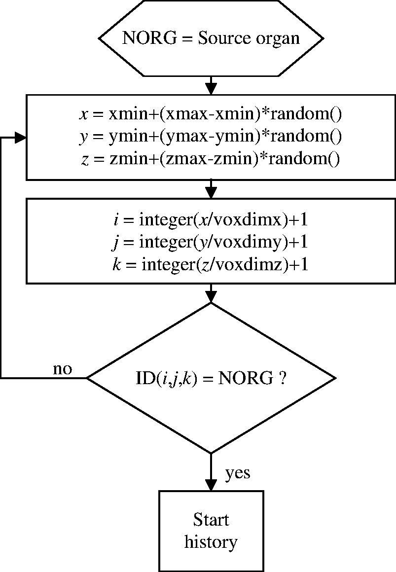
(33) The simplest situation is a single organ that is located at a specific position in the body such as the brain, liver, pancreas, or spleen. The most straightforward sampling method is shown in Fig. 3.7.

Fig. 3.7.

Schematic of Sampling Algorithm A.

3.3.2. Sampling Algorithm B

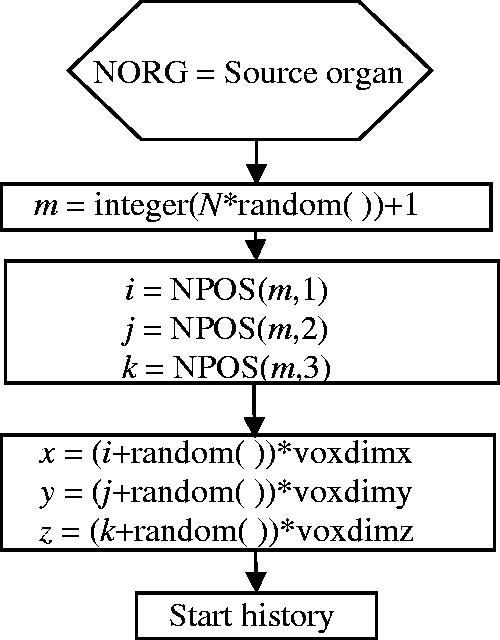
(34) If a source region is distributed throughout the body such as muscle, Sampling Algorithm A may lead to a large proportion of rejected points. In this case, it may be better to use Sampling Algorithm B (see Fig. 3.8).

(35) Let N be the number of voxels belonging to the region in question. These voxels are collected in a separate (N,3)-dimensional array NPOS. The value stored at NPOS(m,1) is the column, NPOS(m,2) is the row, and NPOS(m,3) is the slice where the m^th voxel of the source region is located. To select a voxel, one multiplies N by a random number from the interval (0,1). The nearest integer number above this product is used to identify a source voxel in the NPOS array. x, y, and z co-ordinates are sampled independently inside the selected voxel. All sampled co-ordinate points can be used.

(36) In case the voxel number N of a source region is very large, there is a trade-off between wasted computational time (in the case of Sampling Algorithm A) and large storage requirements (Sampling Algorithm B). Selecting between these algorithms is at the discretion of the user.

Fig. 3.8.

Schematic of Sampling Algorithm B.

3.3.3. Sampling Algorithm C

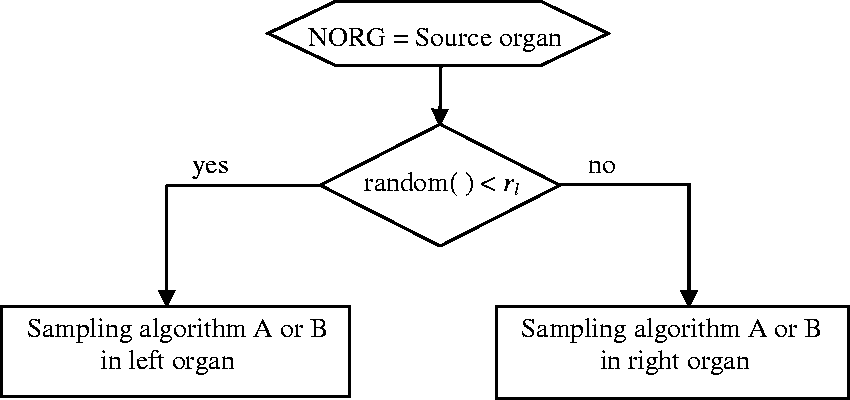
(37) A further common situation is that of an organ pair where both organs are small, but they are relatively distant from each other, such as the adrenals. An efficient sampling algorithm may then be Sampling Algorithm C (see Fig. 3.9), which is a combination of Sampling Algorithms A and B.

(38) Let N_l be the number of voxels belonging to the left organ of an organ pair, Nr the number of voxels belonging to the right organ, N = N_l + Nr the sum of both, and r_l = N_l/N the ratio of the voxel number of the left organ to that of both organs. If a sampled random number r is smaller than r_l, a source point is sampled according to Sampling Algorithm A in the left organ; otherwise, it is sampled in the right organ. This sampling algorithm can be extended to organ groups consisting of more than two parts.

Fig. 3.9.

Schematic of Sampling Algorithm C.

Fig. 3.10.

Schematic of Sampling Algorithm D.

3.3.4. Sampling Algorithm D

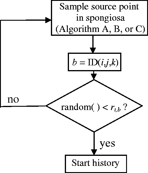
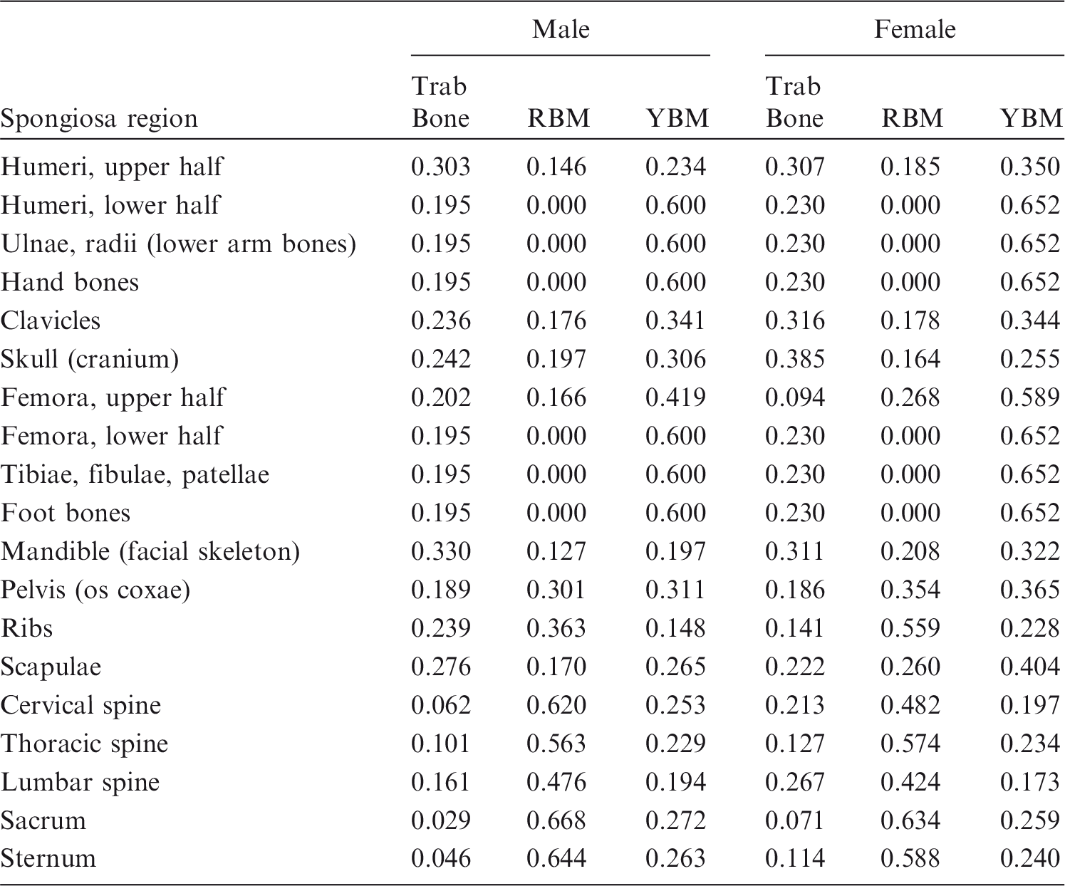
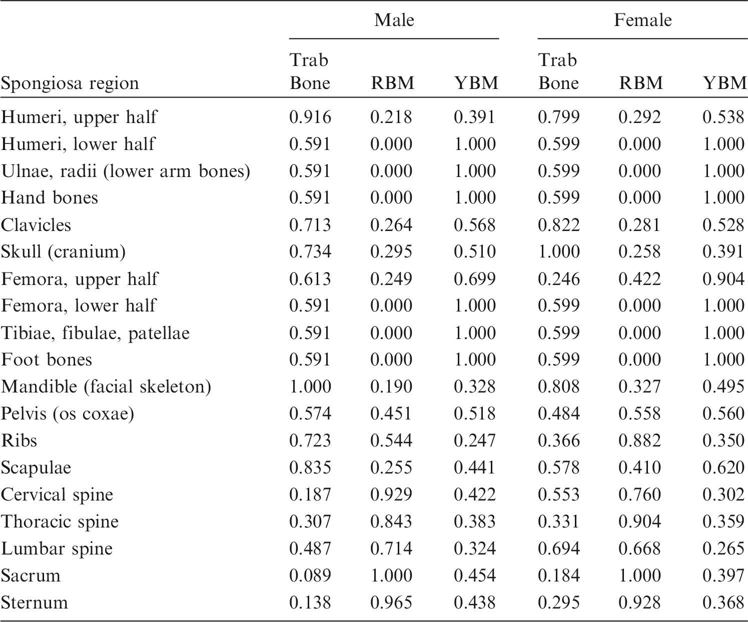
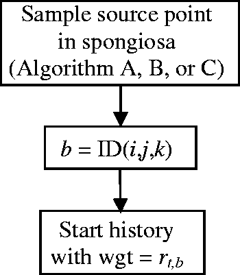
(39) The sampling algorithms mentioned above are for sources distributed homogeneously in the volume of an organ or organ group. There are, however, situations where inhomogeneous source distributions have to be considered. For example, consider a source distributed uniformly in trabecular bone that is not identified uniquely but is included within spongiosa. The same algorithm is equally applicable to marrow sources. There are two main recommended approaches.

(40) In Sampling Algorithm D, the entirety of the segmented spongiosa voxels of all bones serves as the volume in which one samples source points for particle emissions (using Sampling Algorithm A, B or C). However, as the relative amount of trabecular bone in the spongiosa varies between individual bones and bone groups, the source cannot be assumed to be distributed homogeneously in volume. Therefore, the relative amount of trabecular bone in the segmented spongiosa volume of each specific bone or bone group is used as the rejection criterion for accepting source points. Let r_t,b be the relative amount of trabecular bone in the spongiosa of bone (group) b [respective data derived from Tables 3 and 4 in Zankl et al. (2005), see Table 3.1]. If a sampled random number r is smaller than r_t,b, the source point is accepted; otherwise, it is rejected.

(41) Sampling Algorithm D is not optimal as there is a non-zero probability of rejecting a sampled source point for each bone constituent and each spongiosa region. Therefore, these data are normalised to the maximum value of each constituent among all spongiosa regions in Table 3.2. For the spongiosa region with the highest proportion of the respective bone constituent, all sampled source points are accepted; for all other spongiosa regions, the probability of rejection is reduced.

Table 3.1.

Mass ratios of bone constituents [trabecular bone, red bone marrow (RBM), and yellow bone marrow (YBM)] in the spongiosa regions of the reference computational phantoms.

	Male			Female
Spongiosa region	Trab Bone	RBM	YBM	Trab Bone	RBM	YBM
Humeri, upper half	0.303	0.146	0.234	0.307	0.185	0.350
Humeri, lower half	0.195	0.000	0.600	0.230	0.000	0.652
Ulnae, radii (lower arm bones)	0.195	0.000	0.600	0.230	0.000	0.652
Hand bones	0.195	0.000	0.600	0.230	0.000	0.652
Clavicles	0.236	0.176	0.341	0.316	0.178	0.344
Skull (cranium)	0.242	0.197	0.306	0.385	0.164	0.255
Femora, upper half	0.202	0.166	0.419	0.094	0.268	0.589
Femora, lower half	0.195	0.000	0.600	0.230	0.000	0.652
Tibiae, fibulae, patellae	0.195	0.000	0.600	0.230	0.000	0.652
Foot bones	0.195	0.000	0.600	0.230	0.000	0.652
Mandible (facial skeleton)	0.330	0.127	0.197	0.311	0.208	0.322
Pelvis (os coxae)	0.189	0.301	0.311	0.186	0.354	0.365
Ribs	0.239	0.363	0.148	0.141	0.559	0.228
Scapulae	0.276	0.170	0.265	0.222	0.260	0.404
Cervical spine	0.062	0.620	0.253	0.213	0.482	0.197
Thoracic spine	0.101	0.563	0.229	0.127	0.574	0.234
Lumbar spine	0.161	0.476	0.194	0.267	0.424	0.173
Sacrum	0.029	0.668	0.272	0.071	0.634	0.259
Sternum	0.046	0.644	0.263	0.114	0.588	0.240

Table 3.2.

Normalised mass ratios of bone constituents [trabecular bone, red bone marrow (RBM), and yellow bone marrow (YBM)] in the spongiosa regions. Compared with the data of Table 3.1, the entries of each column have been divided by the maximum entry in the respective column.

	Male			Female
Spongiosa region	Trab Bone	RBM	YBM	Trab Bone	RBM	YBM
Humeri, upper half	0.916	0.218	0.391	0.799	0.292	0.538
Humeri, lower half	0.591	0.000	1.000	0.599	0.000	1.000
Ulnae, radii (lower arm bones)	0.591	0.000	1.000	0.599	0.000	1.000
Hand bones	0.591	0.000	1.000	0.599	0.000	1.000
Clavicles	0.713	0.264	0.568	0.822	0.281	0.528
Skull (cranium)	0.734	0.295	0.510	1.000	0.258	0.391
Femora, upper half	0.613	0.249	0.699	0.246	0.422	0.904
Femora, lower half	0.591	0.000	1.000	0.599	0.000	1.000
Tibiae, fibulae, patellae	0.591	0.000	1.000	0.599	0.000	1.000
Foot bones	0.591	0.000	1.000	0.599	0.000	1.000
Mandible (facial skeleton)	1.000	0.190	0.328	0.808	0.327	0.495
Pelvis (os coxae)	0.574	0.451	0.518	0.484	0.558	0.560
Ribs	0.723	0.544	0.247	0.366	0.882	0.350
Scapulae	0.835	0.255	0.441	0.578	0.410	0.620
Cervical spine	0.187	0.929	0.422	0.553	0.760	0.302
Thoracic spine	0.307	0.843	0.383	0.331	0.904	0.359
Lumbar spine	0.487	0.714	0.324	0.694	0.668	0.265
Sacrum	0.089	1.000	0.454	0.184	1.000	0.397
Sternum	0.138	0.965	0.438	0.295	0.928	0.368

3.3.5. Sampling Algorithm E

(42) As with Sampling Algorithm D, the whole spongiosa is taken as the volume from which source points can be sampled. In contrast to Sampling Algorithm D, r_t,b, the relative amount of trabecular bone in the spongiosa of bone (group) b, is not used as a criterion to accept or reject a source point, but each particle starting in the spongiosa volume is assigned this value as its initial ‘statistical weight’.

(43) Sampling Algorithm E is also recommended when the source is the whole body. As homogeneous sources in the whole body should be considered to be distributed homogeneously by mass (not by volume), source points can be sampled uniformly in the whole-body volume, and then the density of the organ/tissue where a source point is located can be assigned a statistical weight to the starting particle history.

(44) Another inhomogeneous source distribution arises when the source is blood. The larger blood vessels have been segmented directly; here, the entire volume is blood source. However, blood distribution inside the organs has been considered by including a respective proportion of blood in the tissue composition of each organ. Therefore, when a blood source has to be sampled, each organ contributes with the fraction of its mass that is due to blood. The blood fractions of the different tissues may be derived from data given in Annex A. In this case, either Sampling Algorithm D or Sampling Algorithm E is recommended.

Fig. 3.11.

Schematic of Sampling Algorithm E.

4. Computational methods for skeletal tissues

(45) For radiological protection purposes, the Commission defines two skeletal cell populations of dosimetric interest relevant to stochastic biological effects: (i) haematopoietic stem cells associated with the risk of radiogenic leukaemia; and (ii) osteoprogenitor cells associated with the risk of radiogenic bone cancer. While data now show that haematopoietic stem cells are found preferentially near the surfaces of the bone trabeculae within skeletal spongiosa (Watchman et al., 2007; Bourke et al., 2009), current modelling for radiological protection assumes these cells to be distributed uniformly within the marrow cavities of haematopoietically active marrow. For the osteoprogenitor cells, the Commission had previously defined their location as a single cell layer within trabecular and cortical endosteum, each 10 µm in thickness, and located along the surfaces of the bone trabeculae and Haversian canals, respectively (ICRP, 1977). In Publication 110 (ICRP, 2009), the surrogate target tissue for the osteoprogenitor cells was redefined as being 50 µm in thickness along the surfaces of the bone trabeculae in skeletal spongiosa, and along the inner surfaces of the medullary cavities in the shafts of all long bones. As a result, cortical bone and its cells within the Haversian canals are no longer considered to be a target tissue for dose assessment. In this publication, the revised 50 -µm surrogate target tissue for the osteoprogenitor cells is termed ‘endosteum’ and is given the symbol TM₅₀ (total marrow within a 50 -µm thickness of the bone surfaces). The term ‘bone surfaces’ is no longer used to describe the target cell layer of relevance to radiogenic bone cancer.

(46) Neither of these skeletal target tissues at radiological risk can be represented geometrically within the voxel structure of the ICRP reference phantoms. As presented above, the skeleton in the male and female reference computational phantoms is described by voxels defining either cortical bone, medullary marrow, or trabecular spongiosa. The latter is a homogeneous mixture of its microscopic tissue constituents – bone trabeculae, active marrow, and inactive marrow – and thus varies in both elemental composition and mass density across different bones of the skeleton in each reference phantom. Computational algorithms must therefore be applied to relate the absorbed dose to spongiosa and medullary marrow to the absorbed dose to either active marrow or endosteum. The elemental compositions of the constituent tissues of trabecular spongiosa are given in Table 3.1 of Publication 116 (ICRP, 2010). It is further noted that the elemental composition of endosteum is equal to that of the active marrow/inactive marrow mixture in a particular skeletal site, as determined by its reference marrow cellularity given in Publication 70 (ICRP, 1995).

4.1. Models for electron transport

(47) Computations of SAFs for charged particles originating within skeletal tissues require detailed geometrical data on both: (i) the bone macrostructure (i.e. regions of spongiosa, cortical bone, and medullary marrow); and (ii) the bone microstructure (i.e. regions of trabecular bone, active bone marrow, and inactive bone marrow). While the former can be modelled properly with the structure of the Publication 110 (ICRP, 2009) reference computational phantoms, the latter requires additional geometric data for radiation transport within the trabecular spongiosa. In this publication, the micro-CT imaging data of Hough et al. (2011) were used for radiation transport simulation in 38 cored samples of spongiosa imaged under micro-CT at an isotropic resolution of 30 µm. The radiation transport code EGSnrc was used under paired-image radiation transport to follow individual electrons simultaneously through both the 3D geometry of ex-vivo CT images of the harvested bone sites, and the 3D geometry of the segmented micro-CT images of spongiosa (Hough et al., 2011). Marrow voxels of the latter were tagged randomly as either active or inactive marrow to achieve reference cellularities for each bone site. Radiation transport results were reported as absorbed fractions for electrons over the energy range of 1 keV to 10 MeV. Source regions included bone marrow (both active and inactive), trabecular bone (both volumes and surfaces), and cortical bone (both volumes and surfaces). The method utilised in Hough et al. (2011): (i) accounts explicitly for electron escape from spongiosa; (ii) includes explicit consideration of spongiosa cross-fire from cortical bone; and (iii) adopts the revised 50 -µm thickness of the endosteum target for risk of bone cancer. SAF values reported in this publication are ratios of the absorbed fractions calculated in Hough et al. (2011), and reference skeletal tissue masses for Reference Adult Male and Reference Adult Female as defined in Publication 110 (ICRP, 2009).

4.2. Models for recoil proton transport following neutron interactions

(48) Computations of absorbed fractions of energy for recoil protons originating in the skeleton have been performed using linear pathlength techniques. These techniques were first developed and described by Spiers’ group (Spiers, 1968; Darley, 1972; Whitwell, 1973; Beddoe et al., 1976; Whitwell and Spiers, 1976; Spiers and Beddoe, 1977; Spiers et al., 1978a,b, 1981; Beddoe and Spiers, 1979), subsequently refined by Eckerman and Stabin (2000) and Bouchet et al. (1999), and most recently revisited by Jokisch et al. (2011a,b). This method was also the basis for recoil proton absorbed fractions used in neutron dose–response functions as summarised in Annex E of Publication 116 (ICRP, 2010). Distributions of linear pathlength segments across trabecular bone and marrow (inclusive of all soft tissue components) were obtained from the high-resolution micro-CT images via digital measurement techniques described in Rajon and Bolch (2003) and Rajon et al. (2002), and published for the 40-year-old male cadaver (Jokisch et al., 2011b).

(49) These two pathlength distributions for a given skeletal site were used in an algorithm (Jokisch et al., 2011a,b) that uses the continuous slowing down approximation (CSDA) range of the charged particle of interest to compute fractional energy deposition in the various skeletal tissues. This algorithm includes a basis for dividing the total marrow space (TMS) into active and inactive components based on typical sizes of skeletal adipose (Reverter et al., 1993). The endosteum (TM₅₀) portion of the TMS path length is determined via an algorithm developed by Jokisch et al. (2011a).

(50) Range/energy data for protons using the CSDA were obtained from ICRU Report 49 (1993). Bragg-Kleeman scaling techniques described in Tsoulfanidis (1983) were utilised to convert ICRU Report 49 water to ICRU Report 46 (1992) adult red marrow (used for active marrow) and adult yellow marrow (used for inactive marrow). ICRU Report 49 compact bone was scaled to yield data for ICRU Report 46 adult cortical bone.

(51) When multiple trabecular cores comprise a single skeletal site, a source mass-weighted average absorbed fraction of the constituent samples, x, was computed as:

${\phi }_{\mathrm{site}}(r_{\text{T}}\to r_{\text{S}})=\sum _x\frac{m_{x,S}}{m_{\mathrm{site},S}}{\phi }_x(r_{\text{T}}\to r_{\text{S}})$

(4.1)

where $\frac{m_{x,S}}{m_{\mathrm{site},S}}$ is the fraction of total site source mass in sample x. Note that this method was also utilised to compute a skeletal averaged absorbed fraction using results from all skeletal sites.

4.3. Models for alpha particle transport

(52) Computations of SAFs of energy from alpha particles (2.0–12.0 MeV) originating in the skeleton were performed using three models: (1) the pathlength-based CSDA model described in Paragraphs 49 and 50 but adapted for alpha particles; (2) a model performing CSDA range-based transport in voxelised images; and (3) a model using MCNPX (Waters, 2002; Pelowitz, 2008) alpha particle transport in voxelised images.

(53) The first two models used identical CSDA range/energy data but differed slightly in their input geometry. While they both used data from the same 40-year-old male cadaver, the second model used the 3D voxelised image for the transport geometry, whereas the first model used pathlength distributions obtained from those images. The second and third models used identical transport geometries (the voxel image) but differed in radiation transport (CSDA vs MCNPX). As a result of the difference in geometry input, the pathlength model differed slightly from the voxel models in modelling of the endosteum target (TM₅₀), inactive marrow constituent, and the algorithm for modelling radiation originating on the trabecular bone surface (TBS).

(54) These differences form the basis for the recommended use of one model over another, or averaging the results of two models for particular source/target combinations. For alpha particles originating in the active marrow irradiating the active marrow (AM←AM), the pathlength model was used as it is thought to have a more realistic modelling of the inactive marrow constituent. For a surface source irradiating the active marrow (AM←TBS), the CSDA voxel model was used as it has a marrow cellularity near the surface consistent with the cellularity of the entire marrow space. For the same reason, the CSDA voxel model was also used for alpha particles originating in the active marrow irradiating the endosteum (TM₅₀←AM). For the remaining endosteum (TM₅₀) target geometries, an average of the pathlength and voxel model results was used, as differences were observed but no basis for preference was determined. Finally, for the remaining active marrow target geometries, no significant differences were observed between the models.

4.4. Response functions for photon and neutron dose to skeletal tissues

(55) As noted above, the tissues of the skeleton at radiological risk, and hence assigned tissue weighting factors w_T, cannot be represented geometrically in the ICRP reference computational phantoms. The energy deposition in these tissues is influenced by their proximity to those of different densities and elemental compositions. This energy deposition can, however, be derived during the Monte Carlo calculations of photon transport through scaling the calculated photon fluence in different skeletal regions (spongiosa or medullary cavities) by functions representing the absorbed dose to the target tissue per photon (Eckerman, 1985; Eckerman et al., 2008; Johnson et al., 2011) or neutron fluence (Bahadori et al., 2011). These functions, referred to as ‘response functions $R$ ’, are derived using models of the microscopic structure of bone geometry of different skeletal regions and the transport of the secondary ionising radiations through those geometries. For photons, these secondary radiations are electrons and positrons, whose absorbed fractions within skeletal tissues were developed in Hough et al. (2011). For neutrons, there are several secondary radiations, the most important of which are recoil protons due to their lower linear energy transfer and thus longer range within trabecular spongiosa (Jokisch et al., 2011a). In this work, all photon SAFs for target regions in the skeleton were derived using EGSnrc tabulations of energy-dependent photon fluence and photon skeletal dose–response function presented in Annex D of Publication 116 (ICRP, 2010). Similarly, all neutron SAFs for target regions in the skeleton were derived using MCNPX tabulations of energy-dependent neutron fluence and neutron skeletal dose–response functions presented in Annex E of Publication 116 (ICRP, 2010).

5. Computational methods for the respiratory tract

(56) Many of the electron and alpha particle absorbed fractions tabulated in Appendix H of Publication 66 (ICRP, 1994a) for the respiratory tract were adopted directly in this publication, with the following exceptions:

revisions to the respiratory tract particle transport model (ICRP, 2015) required changes in dosimetric assumptions regarding the bronchial and bronchiolar regions; and

Publication 66 electron SAFs were augmented with selected values from the reference computational phantoms in cases where the absorbed fractions had previously been assumed to be either unity or zero.

(57) Revisions in the structure of the HRTM, particularly to the particle transport model in the bronchial (BB) and bronchiolar (bb) regions, meant that the dosimetric model for these sources had to be reconsidered. The original HRTM included particle-size-dependent slow clearance compartments, BB₂ (bronchial) and bb₂ (bronchiolar). Material that cleared rapidly from these regions was represented by corresponding compartments BB₁ and bb₁. Activity associated with the slow compartments was assumed to be distributed within the ciliated sol layer adjacent to the airway walls, and activity in the fast compartments was taken to be dispersed throughout the mucous gel overlaying the sol (ICRP, 1994a). The size-dependent slow clearance compartments were eliminated in the revised HRTM (ICRP, 2015), leaving a single phase of clearance in both regions. Owing to uncertainties in both (1) the location of the activity being cleared in mucus relative to the target cells within the airway walls, and (2) values of the mean thicknesses of the two mucous layers, activity in the revised BB and bb compartments is taken to be uniformly distributed throughout both the gel and sol layers. The absorbed fractions for the new single phase of clearance are weighted averages of those for the original fast (gel) and slow (sol) compartments. The weights for the relative thicknesses of the gel and sol layers are 5/11 and 6/11, respectively, for the bronchial region BB, and 2/6 and 4/6, respectively, for the bronchiolar region bb (ICRP, 1994a). Thus, the revised electron and alpha particle absorbed fractions for bronchial and bronchiolar surface sources are given by:

$$\phi (r_{\text{T}}\to \mathrm{BB})=(\frac{5}{11})\phi (r_{\text{T}}\to {\mathrm{BB}}_1)+(\frac{6}{11})\phi (r_{\text{T}}\to {\mathrm{BB}}_2)$$

(5.1)

$$\phi (r_{\text{T}}\to \mathrm{bb})=(\frac{2}{6})\phi (r_{\text{T}}\to {\mathrm{bb}}_1)+(\frac{4}{6})\phi (r_{\text{T}}\to {\mathrm{bb}}_2)$$

(5.2)

where r_T denotes the appropriate target tissue.

(58) The Publication 66 (ICRP, 1994a) electron SAFs were supplemented with extra cross-fire terms (when absorbed fraction = 0) or improved self-dose values (when absorbed fraction = 1) derived from electron transport calculations in the male and female reference computational phantoms. For many organs in the reference phantoms, the SAFs computed for self-irradiation were approximately inversely proportional to mass, with only minor or moderate deviations from mass scaling. This could be exploited in instances of self-irradiation in the HRTM, where target cells are located accurately in the phantom but with inadequate voxel resolution by correcting the SAFs with the reference mass. This applied to alveolar-interstitial and extrathoracic lymph node sources, replacing the original default assumption that the absorbed fraction = 1 for these cases and allowing for energy-dependent electron escape.

(59) Electron cross-fire SAFs for many source and target combinations exhibited reciprocity over wide energy ranges, implying that the cross-fire SAFs were independent of source or target masses and did not require mass correction. Consequently, selected values could be used directly to fill any vacancies in the HRTM SAF matrix where cross-fire absorbed fractions had previously been assumed to be zero at all energies.

(60) Alpha particle SAFs were not supplemented in this fashion. The electron and alpha particle absorbed fractions that were adopted from Publication 66 (ICRP, 1994a) were assumed to be gender-independent, but the SAFs derived from them used male or female target masses as appropriate. For consistency, the derived values were mapped on to the energy grid used for reference phantom radiation transport calculations.

6. Computational methods for the alimentary tract

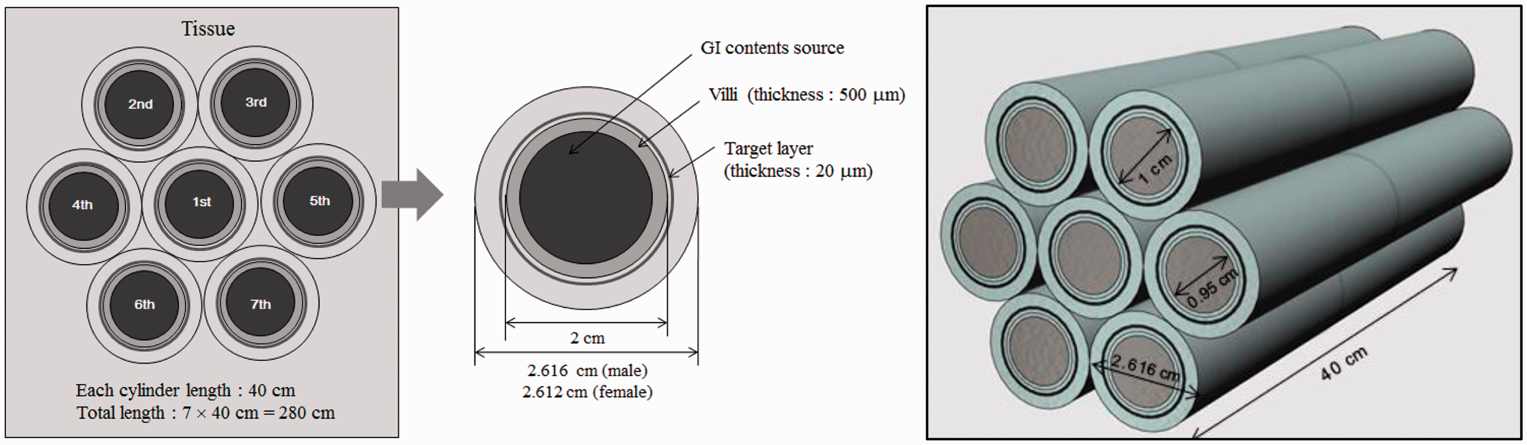
(61) In Publication 100 (ICRP, 2006), the morphometric and dosimetric models of the alimentary tract are defined, including source regions of radionuclide deposition and target regions of radiosensitive stem cells. For electron sources in the alimentary tract, Annex F of Publication 100 provided provisional SAF values based upon Monte Carlo radiation transport simulation in the geometric models. Alpha particle transport was not considered in Publication 100, and thus SAF values of alpha emissions presumed full energy deposition in the source region.

(62) In this publication, new radiation transport simulations were performed for both electron and alpha particle sources using the geometric models described in Section 7.2 of Publication 100 (ICRP, 2006). The one exception was that of the small intestine wall. In Publication 100, a single tubular structure was adopted, while in the present publication, a hexagonal array of tubular structures was adopted to allow for wall segment cross-fire (see Fig. 6.1). All radiation transport simulations were performed using MCNPX Version 2.6 (Pelowitz, 2008). Maximum particle energies considered were 10 MeV for electrons and 12 MeV for alpha particles.

Fig. 6.1.

Schematic of the folded small intestine model used to allow for electron cross-fire. GI, gastrointestinal.

7. Limiting specific absorbed fraction values for electrons, photons, and alpha particles

(63) SAF data for mono-energetic electrons, photons, and alpha particles were calculated using Monte Carlo methods for particles ranging in energy from 0.01 to 10 MeV for electrons and photons and 2.0 to 12.0 MeV for alpha particles. Use of the resultant SAF tabulations in dosimetric calculations necessitates addressing particles of energy less than the lower value in the tabulations. For example, the beta spectra tabulated in Publication 107 (ICRP, 2008) include emissions at energies below 0.01 MeV. The entire beta spectrum of Re-187 lies below 0.01 MeV. Sixty-seven percent of the tritium (H-3) beta emissions are below 0.01 MeV; the mean energy of the spectrum is 5.68 keV and endpoint energy is 18.59 keV. The decay of many radionuclides result in emission of Auger electrons, internal conversion electrons, and photons of energy less than 0.01 MeV. Rather than extrapolate the Monte-Carlo-based SAF to the lower energy emission, the limiting SAF at zero energy has been defined, thus enabling use of interpolation procedures.

7.1. Limiting specific absorbed fraction values for solid source–target regions

(64) For solid target regions (organs), the limiting SAF is non-zero in the case of self-dose, and zero if the two regions are distinct. Denoting the target and source regions as r_T and r_S, respectively, the limiting SAF is:

${lim}_{E\to 0}\mathrm{SAF}(r_{\text{T}}\to r_{\text{S}};E)=\{\frac{1}{M_{r_{\text{T}}}},\text{if}\hspace{0.5em}{r}_{\text{S}}=r_{\text{T}}0,\text{if}\hspace{0.5em}{r}_{\text{S}}\ne r_{\text{T}}$

(7.1)

This procedure has been commonly employed in software, but has not previously been included in SAF tabulations. The procedure is extended to the source–target regions of the HRTM and HATM.

7.2. Limiting specific absorbed fraction values for HRTM source–target regions

(65) The basal and secretory cells of the HRTM airways are the dosimetric target regions of interest. Potential source regions of the airways include activity distributed on the inner surface of the airway, within bound and sequestered regions, and uniformly throughout the wall. The limiting SAF for these target regions and either the inner surface or sequestered region of the airway as the source region is zero, as no target region tissue resides within the source regions. For radiations emitted uniformly within the ET₂ airway wall, the limiting SAF for the basal cell target region of the airway is:

${lim}_{E\to 0}\mathrm{SAF}(\text{ET}2-\text{bas}\to \text{ET}2-\text{wall};E)=\frac{1}{M_{\text{ET}2-\text{wall}}}$

(7.2)

and for lung tissue sources and basal and secretory target regions within the bronchi and bronchiolar airways:

$${lim}_{E\to 0}\mathrm{SAF}(X-\text{bas}\to \text{Lung}-\text{Tis};E)=\frac{1}{M_{\text{Lung}-\text{Tis}}}$$

(7.3.a)

$${lim}_{E\to 0}\mathrm{SAF}(X-\text{sec}\to \text{Lung}-\text{Tis};E)=\frac{1}{M_{\text{Lung}-\text{Tis}}}$$

(7.3.b)

where X represents the acronyms Bronch and Bchiol defined in Tables A.1 and A.2 with their respective mass values.

(66) The basal cells of the ET₂ airway lie within the bound source region of the airway. Thus, the limiting SAF for this source–target pair is:

${lim}_{E\to 0}\mathrm{SAF}(\text{ET}2-\text{bas}\to \text{ET}2-\text{bnd};E)=\frac{1}{M_{\text{ET}2-\text{bnd}}}$

(7.4)

The basal and secretory cells of the bronchi and bronchiolar airways also lie within the bound source region of these airways. Thus, the limiting SAFs for these target regions and the bound source region are:

$${lim}_{E\to 0}\mathrm{SAF}(X-\text{bas}\to X-\text{b};E)=\frac{1}{M_{X-\text{b}}}$$

(7.5.a)

$${lim}_{E\to 0}\mathrm{SAF}(X-\text{sec}\to X-\text{b};E)=\frac{1}{M_{X-\text{b}}}$$

(7.5.b)

where X represents the acronyms Bronch and Bchiol defined in Tables A.1 and A.2 with their respective mass values.

7.3. Limiting specific absorbed fraction values for HATM source–target regions

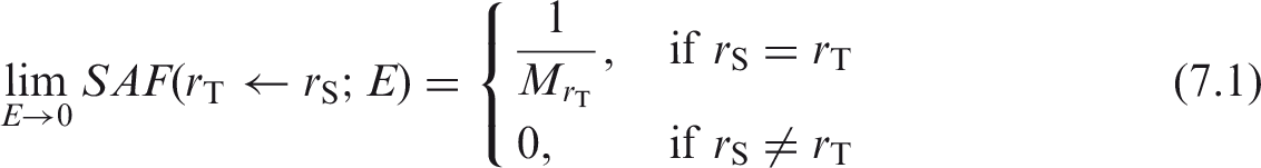
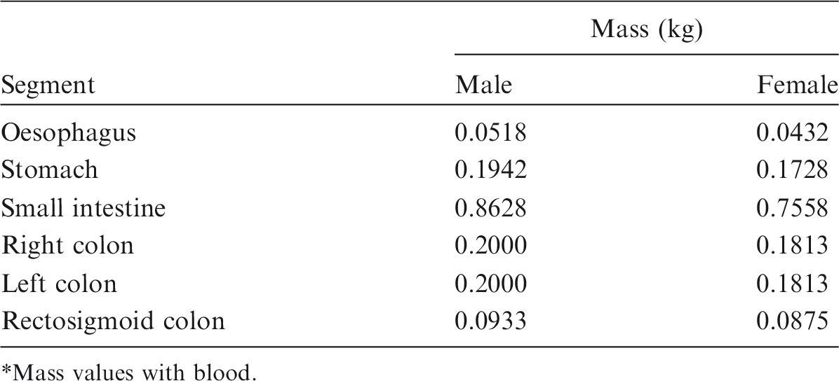
(67) The target regions of the HATM are specified at depths into the wall of each segment of the tract. In addition to the oesophagus, the segments include the stomach, small intestine, right colon, left colon, and rectosigmoid colon, denoted by St, SI, RC, LC and RS, respectively (see Table A.1 or A.2 for additional information). The source regions of the segment include: the contents, the mucosa region, the villi (only in the small intestine segment), and the wall. For each segment, a limiting SAF of zero is assigned when the source region is either the lumen contents (all alimentary tract segments) or the villa (small intestine only). Non-zero limiting values occur for the wall and mucosa as source regions. The non-zero limiting SAFs are:

$${lim}_{E\to 0}\mathrm{SAF}(X-\mathrm{stem}\to X-\mathrm{wall};E)=\frac{1}{M_{X-\mathrm{wall}}}$$

(7.6a)

$${lim}_{E\to 0}\mathrm{SAF}(\mathrm{Oesophagus}\to \mathrm{Oesophag}-w;E)=\frac{1}{M_{\mathrm{Oesophag}-w}}$$

(7.6b)

where X represents the segments other than the oesophagus. The mass of the segment walls are given in Table 7.1. For a source within the mucosa layer of segments other than the oesophagus, the limiting SAFs are:

${lim}_{E\to 0}\mathrm{SAF}(X-\mathrm{stem}\to X-\mathrm{mucosa};E)=\frac{1}{M_{X-\text{mucosa}}}$

(7.7)

where X denotes St, SI, RC, LC, and RS. The mass of the mucosa layer for these segments is given in Table A.3.

Table 7.1.

Mass of Human Alimentary Tract Model segment walls.*

	Mass (kg)
Segment	Male	Female
Oesophagus	0.0518	0.0432
Stomach	0.1942	0.1728
Small intestine	0.8628	0.7558
Right colon	0.2000	0.1813
Left colon	0.2000	0.1813
Rectosigmoid colon	0.0933	0.0875

*

Mass values with blood.

7.4. Limiting specific absorbed fraction values for the blood source region irradiating target regions

(68) The Monte Carlo calculations for a source in blood reflect a consideration of the distribution of blood in the body, including within the target region. The limiting SAF for target region $r_{\text{T}}$ due to blood as a source is:

${lim}_{E\to 0}\mathrm{SAF}(r_{\text{T}}\to \mathrm{Blood};E)=\frac{f_{r_{\text{T}}}}{M_{r_{\text{T}}}}$

(7.8)

where $f_{r_{\text{T}}}$ is the mass fraction of the body’s blood in target $r_{\text{T}}$ , as per Publication 89 (ICRP, 2002) (also see Tables A.1 and A.2 of this publication).

7.5. Low-energy specific absorbed fraction values based on the limiting specific absorbed fraction

(69) The source–target pair records of the SAF files include the limiting SAF at zero energy and SAF values for two additional low energies (i.e. at 0.001 and 0.005 MeV in the case of electrons and photons). For alpha particles, the additional low energies are 1 and 1.5 MeV. If the SAF for the lowest energy of the Monte Carlo calculation is non-zero, SAFs for the two additional energies were derived by log-log interpolation of the limiting SAF and the SAF at the lowest energy of the Monte Carlo calculation.

(70) If the limiting SAF for the source–target pair is non-zero, an energy value of 10⁻⁶ MeV is assumed for the purpose of the log-log interpolation. Similarly, if the limiting SAF is zero, but the Monte-Carlo-based SAF at the lowest energy is non-zero, the log-log interpolation assumed a limiting SAF of 10⁻¹²kg⁻¹ at 10⁻⁶ MeV.