Sage Journals: Discover world-class research

Abstract

Single case research is a viable way to obtain evidence for social and psychological interventions on an individual level. Across single case research studies various analysis strategies are employed, varying from visual analysis to the calculation of effect sizes. To calculate effect sizes in studies with few measurements per time period (<40 data points with a minimum of five data points in each phase), non-parametric indices such as Nonoverlap of All Pairs (NAP) and Tau-U are recommended. However, both indices have restrictions. This article discusses the restrictions of NAP and Tau-U and presents the description, calculation, and benefits of an additional effect size, called the Typicality of Level Change (TLC) index. In comparison to NAP and Tau-U, the TLC index is more aligned to visual analysis, not restricted by a ceiling effect, and does not overcompensate for problematic trends in data. The TLC index is also sensitive to the typicality of an effect. TLC is an important addition to ease the restrictions of current nonoverlap methods when comparing effect sizes between cases and studies.

Keywords

single case research NAP Tau-U effect sizes Typicality of Level Change

Introduction

In intervention studies on complex human behavior in the field of, for example, social work (Wong, 2010), forensic psychology (Spreen et al., 2010), special education (Horner et al., 2005), and counseling practices (Lenz, 2015), Single Case Research (SCR) has been applied. SCR is a viable alternative when between-group studies, such as Randomized Controlled Trials (RCTs), are not possible (Hein & Weeland, 2019). Due to practical reasons, such as difficulties to include sufficient respondents, finding adequate control groups and reluctant patients as forensic patients (Spreen, 1992), the assumptions of between-group studies are sometimes difficult to meet in intervention studies. In such situations, SCR can serve as an alternative, as causal associations can be assessed within the context of an individual or a small group of individuals. SCR enables systematic evaluation of interventions by repeated measurement of an outcome variable in typically one participant (Vannest & Ninci, 2015). The effect of interventions is then defined by the difference in outcomes between the phases in the experimentally controlled conditions. Typically, these conditions comprise A-phases (baseline or control) and B-phases (intervention or treatment) in reversal designs and multiple baseline designs, different conditions B (treatment 1) and C (treatment 2) in alternate treatment designs, or different criterions B (treatment 1) and B’ (reinforced treatment 1) in changing criterion designs (Heyvaert et al., 2015).

Analysis of SCR data usually starts with visual analysis that refers to reaching a judgment about the reliability or consistency of intervention-effects by eye (Kazdin, 2011). Six aspects of the graphical data are to be considered: the difference in mean values between phases (level), the stability of the measure during the phases (variability), the tendency of increasing or decreasing values within phases (trend), the consistency of change between two phases (overlap), the immediacy of the effect (intercept gap), and the replicability of the effect within the design (consistency) (Franklin et al., 1996; Kratochwill et al., 2013; Lane & Gast, 2014). Visual analysis can lead to type I errors when the effects are small to moderate and when data are autocorrelated (Barton et al., 2019; Brossart et al., 2006). Therefore, it is recommended to proceed with statistical analysis for more reliable and standardized decisions about the existence and size of an effect (Kratochwill et al., 2013; Parker & Brossart, 2003; Swann & Pustejovsky, 2018).

For SCR designs with statistical sufficient measurements in all phases, parametric analysis techniques such as standard t or F tests (Barlow et al., 2009), time series analysis (Yaffee & McGee, 2000), Standardized Mean Difference (Busk & Serlin, 1992), Bayesian analysis (Rindskopf, 2014a), multilevel analysis (Baek et al., 2014), randomization tests (Heyvaert & Onghena, 2014), regression analysis (Swaminathan et al., 2014), Generalized Least Squares analysis (GLS; Swaminathan et al., 2014), Hierarchical Linear Modeling (HLM; Gage & Lewis, 2014), and d-statistics (Shadish et al., 2014) can be used. For a more complete picture there are overviews of statistical techniques that can be used in SCR designs (see Manolov & Moeyaert, 2017). Most parametric tests are valid if strict distributional assumptions are met. Severe outliers, unbalanced variance between phases, no variance in one or more phases, or an insufficient number of measurements in the study or in one of the phases, would make it doubtful to use most parametric tests to provide valid results (Heyvaert & Onghena, 2014).

Current What Works Clearinghouse standards (WWC-standards) recommend reporting a d-statistic as effect size in SCR designs (What Works Clearinghouse [WWC], 2020). This is useful because the d-statistic is comparable across designs and the results are comparable to effect sizes in group designs (Shadish et al., 2014). To obtain this parametric statistic, the standard deviation across participants is used, rather than the standard deviation within participants (Odom et al., 2018).

In many SCR intervention studies, the assumptions to validly compute parametric effect sizes cannot be met because of too few data points. As mentioned earlier, this causes problems for parametric testing due to severe outliers, unbalanced variance between phases, or no variance in one or more phases. For research situations where less than 40 data points with a minimum of five data points are collected in each phase, non-parametric effect size indices are recommended. Percentage of Nonoverlapping Data (PND; Scruggs et al., 1987) has been one of the most widely used non-parametric effect sizes in SCR for a long time (Heyvaert & Onghena, 2014). However, this index does not always reflect the correct effects for outliers or because adverse effects due to treatment and trend are present. Also, PND cannot discriminate when there is complete nonoverlap. To address these limitations, modifications of PND have been developed, such as the Nonoverlap of All Pairs (NAP; Parker & Vannest, 2009) and Tau-U (Parker et al., 2011).

Both NAP (e.g., Abrahamsson et al., 2018; Baldwin & Powell, 2015; Collier-Meek et al., 2019; Jamieson et al., 2019; Spauwen et al., 2020) and Tau-U (e.g., Brodhead et al., 2019; Erhardsson et al., 2020; Kunze et al., 2021; McGoldrick et al., 2021) are frequently used in SCR designs with small data sets. Both measures include one or two of the six aspects of the data that are assessed in visual analysis (Tanious et al., 2020). Because of the emphasis on nonoverlap and trend, other aspects of visual analysis of the data, such as immediacy of the effect and level change, are unweighted in the effect size (Dart & Radley, 2017) or only indirect by nonoverlap.

To tackle these restrictions, we introduce the Typicality of Level Change (TLC) index that does consider all six aspects of visual analysis. First, we discuss the restrictions NAP and Tau-U have in correctly differentiating effect sizes between cases and studies. Next, we introduce the concept of Typicality of Level Change (TLC). Based on a hypothetical example of a non-concurrent multiple baseline design and an ABAB-design, we argue how TLC complements visual analysis regarding the restrictions of NAP and Tau-U. Although our example comprises two designs, TLC can be applied in any of the SCR designs that have two-phase comparison as the basic unit of analysis.

Restrictions of Nonoverlap Indices: Nonoverlap of All Pairs (NAP) and Tau-U

NAP uses the degree of overlap of data between two phases to express effect sizes (Parker & Vannest, 2009). NAP compares all data in the baseline phase with all data in the intervention phase. Whenever values in the intervention phase (B) exceed the values in the baseline phase (A), values of “1” are assigned; whenever values in B are smaller than values in A, values of “0” are assigned, and when values in both phases are identical, values of “0.5” are assigned. The assigned values for each pair of A- and B-data are added and divided by the total number of pairs between the two phases (Vannest & Ninci, 2015). Consequently, NAP is a value that varies between 0 and 1 (0 = decline without overlap between phases, 0.5 = as much overlap as nonoverlap between phases, 1 = increase without overlap between phases).

However, NAP has at least three restrictions. Firstly, NAP suffers from a ceiling effect. Beyond the point where there is complete nonoverlap between two phases the magnitude of level change is ignored (Parker et al., 2011). Parker et al. (2011) found that of the 176 data sets from a convenience sample of published articles using AB designs, 25% of these data sets yielded a maximum NAP (NAP = 1.00). The level change, immediacy of effect and trends differ between the studies despite a NAP of 1.00. With respect to level change, this means that a client whose condition improved from very dissatisfied to very satisfied and a client whose condition improved from very dissatisfied to dissatisfied can both receive a NAP of 1.00, while the magnitude of change in their conditions is clearly different. Secondly, because trend is not fully adjusted for by NAP, NAP is susceptible for overestimating the size of effects when trend is present (Parker et al., 2011). For a client already improving before the start of the intervention and continuing to improve during the intervention, NAP would lead to an overestimation of the size of the effect. Thirdly, there is the problem that we refer to as the problem of typicality. NAP does not account for the varying probabilities on nonoverlap between cases due to different baseline scores. When a client already has a relatively high score at baseline, it is statistically more difficult to improve compared to a client who has a relatively low score at baseline. Thus, it becomes more difficult or even impossible to exceed baseline data when scores are relatively close to the optimum at baseline. This means that the amount of possible change depends on baseline levels. The ceiling effect, problems to adjust for trend, and the problem of typicality, restrict NAP to properly compare the size of effects between studies or cases.

In contrast to NAP, Tau-U (Parker et al., 2011) adjusts for trend in the data in the baseline and intervention phase based on nonoverlap (Vannest & Ninci, 2015) and has different versions. The version used in this study is the initial version, called Tau-U_AB, that adjusts for trend in both the baseline and intervention phase (Vannest & Ninci, 2015). Other versions contain an adjustment for baseline trend only (Davis, 2014; Parker et al., 2011; Rakap, 2015). All versions are computed in the same way as the NAP and correct for trend in the baseline and/or intervention phase. This means that NAP is extended with comparisons of ties within phases, in the same way as is used in the calculation of Kendall’s Rank Correlation (KRC). Overlap between phases, positive trend during baseline and negative trend during intervention hinder the validity of the argument that behavior has changed because of the intervention. The three counterparts (nonoverlap between phases, the absence of positive trend during baseline phase, and the absence of negative trend during intervention phase) are aggregated and divided by the sum of pairs to obtain Tau-U_AB (Supplement 1 illustrates the computation).

By taking both nonoverlap and trend into account, two of the restrictions of NAP do not apply to Tau-U: (1) it discriminates between effect sizes beyond the point of nonoverlap, making the ceiling effect less problematic (Parker et al., 2011), and (2) it corrects for trend. However, known restrictions include dependency on phase length with respect to its correction of trend, doubtful alignment with visual analysis, vague or inconsistent terminology in SCR publications related to Tau-U, and the difficulty of graphing (Brossart et al., 2018; Tarlow, 2017). By adjusting for trend in situations with immediate and large level change, the correction can lead to counter-intuitive results. Consequently, Tau-U underestimates effect sizes when large immediate level changes occur in combination with a moderate trend. Like the NAP, the problem of typicality is also not covered by Tau-U.

The Typicality of Level Change Index

The Typicality of Level Change (TLC) index was developed to ease the restrictions of NAP and Tau-U. TLC is based on the logic of combinatorial inference in typicality tests (Rouanet et al., 2000). In such tests, from a known reference distribution of some statistic (such as the mean of a variable) a particular subset of size n is compared with all other samples of size n that are possible from the reference distribution. The proportion of samples that exceed the value of the particular sample expresses its typicality within the reference distribution. The smaller this proportion, the more atypical the particular sample. The TLC index can be computed for single case studies in which measurements of some numerical outcome variable is compared between two phases. The reference distribution is then defined as the combination of all possible values of the outcome variable between the n measurements (Figure 1).

Figure 1.

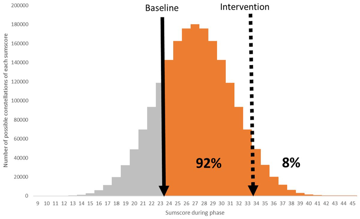
Visual illustration of a TLC of 0.92. The complete distribution of possible sum scores is the reference distribution, in this example based on five measurements with an outcome variable on an ordinal measurement scale from 1 to 9. The baseline sum score was 23 and the intervention sum score improved to 34, achieving 92% of the maximum possible improvement.

TLC is the percentage achieved improvement from the maximal possible improvement given the baseline score in the reference distribution. TLC can be calculated in an Excel spreadsheet (Supplement 3 provides a link to the sheet). Consider Figure 1, which shows the reference distribution of all sum scores which are possible by combining five measurements of an outcome variable having a scale of 1 to 9, resulting in a minimum score of 5 and a maximum of 45. Suppose in a single case study that the sum score of five measurements of the baseline phase was 23 and of five measurements during the intervention phase 34. The gray area in Figure 1 represents all sum scores that do not exceed the observed baseline sum score (maximal 23). The part of the reference population in which the sum scores exceed the baseline score and thus indicate an improvement is illustrated by the orange area (greater than 23). This improvement area can be divided into two parts. The orange area left to the intervention sum score, the numerator in the formula of TLC (Supplement 3), represents all sum scores between the baseline sum score and the achieved intervention sum score of 34. TLC is calculated as the percentage of the achieved improvement in the orange area. For Figure 1 TLC is 0.92, meaning that of the maximum possible change based on his baseline score, this participant achieved 92%. The remaining 8%, the orange area right to the intervention sum score, is what separates the participant from the optimal score.

Typical Values of TLC

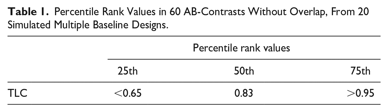
To explore what TLC outcomes may account for small, medium, or large effect sizes, we simulated data. In this study 20 SCR Designs having three nonoverlapping AB-contrasts each (multiple baseline designs with three participants) were simulated. The simulated designs had a phase length of minimum 3 and maximum 10 in each phase (meeting WWC-standards with reservations at least [Kratochwill et al., 2013]), and a measurement scale varying from a 5 point scale to a 12 point scale. All contrasts were completely nonoverlapping (NAP = 1). From the simulation we deduced typical values for small, medium, and large effect sizes of TLC. We used the same critical intervals as for benchmarks of NAP were obtained (Parker & Vannest, 2009). Figure 2 shows how TLC discriminates between samples without any overlap, with typical values of the percentiles being 0.65 for 25th, 0.83 for 50th, and 0.95 for 75th (Table 1).

Figure 2.

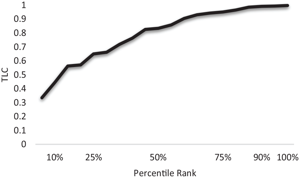
Uniform probability plot for TLC of 60 AB-contrasts without overlap, from 20 simulated multiple baseline designs.

Table 1.

Percentile Rank Values in 60 AB-Contrasts Without Overlap, From 20 Simulated Multiple Baseline Designs.

	Percentile rank values
	25th	50th	75th
TLC	<0.65	0.83	>0.95

Confidence Intervals of TLC

To obtain confidence levels to estimate the precision of the effect size (Vannest & Ninci, 2015), a modified jack-knife principle can be employed (Snijders & Borgatti, 1999). The basic idea of the jack-knife principle is to create a number of N_i artificial data sets from N sample elements, by excluding the i-th element. If a sample consists of elements A, B, C, D, and E, then one of the five artificial data sets consists for example of elements A, B, D, and E. The variability between the artificial data sets indicates the variability that may be expected when new data is collected from replicated studies. TLC is not calculated from one sample with size N but from two samples, consisting of size N₁ and N₂, respectively belonging to the baseline and intervention phase. Jack-knife would result in calculating the TLC for all different combinations of n₁ possible samples of size N₁−1 and n₂ possible samples N₂−1, such that n = n₁ × n₂. If the standard error of TLC, for example, is calculated by comparing five baseline samples and five intervention samples, 25 sample contrasts are made to calculate the standard error:

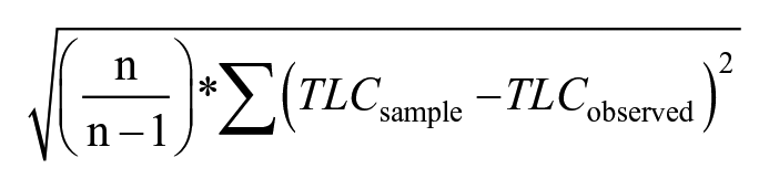
\sqrt{(\frac{n}{n - 1}) * \sum^{} {(T L C_{sample} - T L C_{observed})}^{2}}

This routine would mean that n₁ × n₂ calculations have to be made, which is very intensive especially when the number of measurements and the number of answer categories grow. Therefore, one could alternatively look at the 2.5 and 97.5 percentiles of the empirical distributions from the sample produced by the simulation of n₁ × n₂ samples. This technique is often used with Markov Chain Monte Carlo simulations (Rindskopf, 2014b). Since in the distribution of the example, 25 sample contrasts are created, the 2.5 and 97.5 percentiles are given by the minimum and maximum of these samples. The confidence interval (CI) of the TLC (0.92) in Figure 1 is [0.81, 0.95]. Calculating the confidence levels gives an indication of the precision of the effect and makes it possible to compare effects across cases. Calculation of the CI is shown in Supplement 2.

Material and Methods

To illustrate the usefulness of the TLC-index as an additional effect measure to NAP and Tau-U, consider the following two hypothetical studies. Study 1 consists of a non-concurrent multiple baseline design (MBD) to assess the functional relationship between intervention X and the quality of life in individuals with dementia. Participants are three elderly people, named Anne, Bob, and Chris. During a baseline period of 5, 7, and 9 weeks, baseline data is collected by weekly administration of a simple Quality of Life (QoL) question. The participants are asked “Taking everything in your life into account, please rate your overall Quality of Life on the following 10-point scale,” with 1 meaning “very distressing,” 5 to 6 “so-so,” and 10 “great.” After the baseline phase, the intervention period that lasts for the remaining of the 14 weeks started. For the sake of argument, it is assumed that further criteria for causal inference according to WWC-standards (WWC, 2020) are met.

Study 2 consists of an ABABAB withdrawal design to assess the functional relationship between intervention X and quality of life in individuals with dementia. The intervention X in study 2 is the same intervention as in study 1. In this case there is only one participant, an elderly lady called Jennifer. During the study, data is collected weekly by taking the same QoL-question during six phases: a baseline period of 5 weeks, a first period of intervening of 9 weeks (the first B), withdrawals of the intervention (the second and third A), and re-introductions of the intervention (the second and third B). Intervention X is supposed to have no learning effect: the withdrawal of the intervention should lead to a decline of quality of life back to baseline level, allowing for ABABAB design.

We constructed data for each case in the two studies, in a way that would show (a) how TLC can be used in different high validity designs, such as ABABAB designs and MBDs, and (b) how TLC deals with the restrictions of the NAP and Tau-U. Both studies contained at least three AB-replications: each of the participants in the MBD-study (Anne, Bob, Chris) and five phase changes in the ABABAB-study (of which we analyze A1B1, A2B2, and A3B3; B1A2 and B2A3 are ignored because of comparability of the two designs). We constructed data so that those replications are similar, but with subtle differences in pairs of replications with respect to the mean difference and trend. The first pair (Anne vs. A1B1) and the second pair (Bob vs. A2B2) differ with regard to mean level and trend in the first phase, and the third pair with regard to the typicality of the change (Chris vs. A3B3).

In Table 2, the manipulated characteristics of the data for each of the participants are shown. As an illustration, for case Bob, this means that his scores on QoL increases from baseline to intervention (small positive level change), with no overlap between phases and no large deviations within the phases (small variability). During baseline, scores did not show an upward or downward tendency (no positive trend). Also, there is an instant gap between baseline and intervention, (immediate change). The designs contain multiple phase shifts that show replications of an effect (consistency) between (MBD-study) and within participants (ABABAB-study).

Table 2.

Characteristics of the Data of the Two Studies Based on the Six Elements in Visual Analysis (Vannest & Ninci, 2015).

	Level-change	Immediacy	Overlap	Baseline trend	Variability	Consistency
Study 1	Increase (+)	Yes	Complete nonoverlap	No concern	Small	Yes, 3 supporting replications
P1: Anne	Small +	Yes	Complete nonoverlap	Unproblematic	Small
P2: Bob	Small +	Yes	Complete nonoverlap	Unproblematic	Small
P3: Chris	Medium +	Yes	Complete nonoverlap	Unproblematic	Small
Study 2	Increase (+)	Yes	Complete nonoverlap	Slight concern	Small	Yes, 3 supporting replications
R1: A1B1	Large +	Yes	Complete nonoverlap	Slight concern	Small
R2: A2B2	Large +	Yes	Complete nonoverlap	Slight concern	Small
R3: A3B3	Medium +	Yes	Complete nonoverlap	Unproblematic	Small

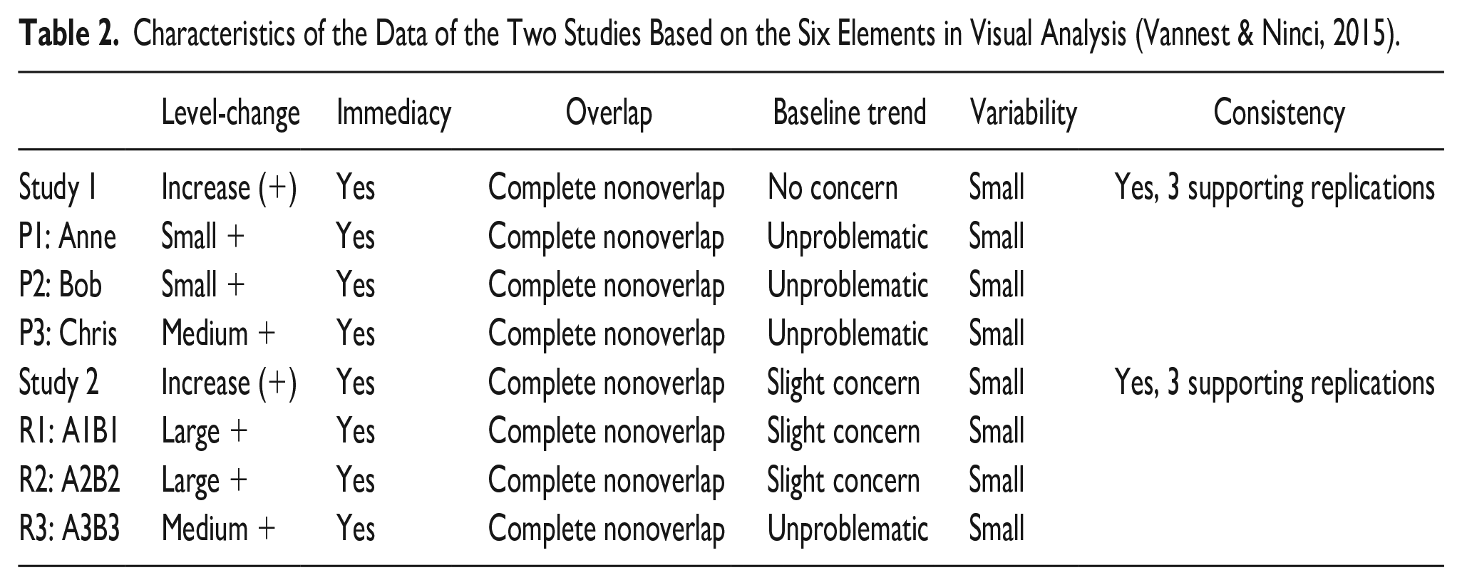
The effect sizes NAP, Tau-U, and TLC are calculated for each of the participants. Averaging the measures gives an indication of the functional relation between the intervention and QOL. Next, we focus on how the indices differentiate effect sizes between the participants. NAP, Tau-U, and TLC are compared on the three theoretical restrictions mentioned before: ceiling effect, correction for trend, and typicality. Computations were performed in Excel. Pairs of participants are compared to show how the indices differ from each other. The differences are compared with the conclusions from visual analysis, in which all relevant characteristics of the data can be justified.

Results

The change in QoL of the three participants in Study 1 and over phases in Study 2, divided into three AB contrasts, is illustrated in Figure 3. Trend lines are only included in the top four panels, the two panels in the bottom row do not have trends.

Figure 3.

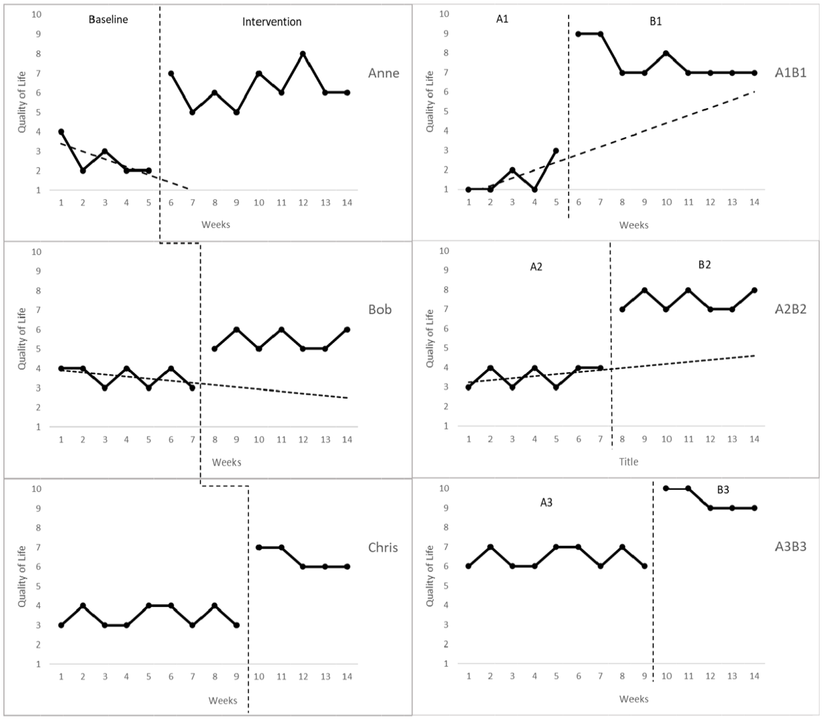
Three replications of the effect in the multiple baseline design (study 1, left panels) and the ABABAB-design (study 2, right panels).

To compare the magnitude of effects between the participants, NAP, Tau-U, and TLC are calculated for each of the phase shifts (Table 3). We rather compare two phases than the whole design, because each replication should reflect evidence, and the design could be hard to comprehend without looking to the individual phase shifts first.

Table 3.

Effect Sizes NAP, Tau-U, and TLC on Average and for Each of the Phase-Shifts in the Studies, With Indication of the Effect Size According to the Benchmarks Obtained in the Simulation in This Study.

	Mean A	Mean B	Trend A^a	Trend B^a	NAP	Tau-U_AB	TLC [low, high]	Effect size TLC
Study 1	3.20	5.98	−0.24	−0.15	1.00	0.54	0.71 [0.65, 0.75]	Medium
Anne	2.60	6.11	−0.50	0.06	1.00	0.59	0.79 [0.72, 0.90]	Medium
Bob	3.57	5.43	−0.29	0.10	1.00	0.63	0.49 [0.44, 0.54]	Small
Chris	3.44	6.40	0.06	−0.60	1.00	0.41	0.85 [0.78, 0.87]	Medium
Study 2	3.87	8.13	0.28	−0.31	1.00	0.39	0.99 [0.98, 0.99]	Large
A1B1	1.60	7.56	0.50	−0.44	1.00	0.26	0.99 [0.97, 1.00]	Large
A2B2	3.57	7.43	0.29	0.10	1.00	0.49	0.98 [0.98, 0.99]	Large
A3B3	6.44	9.40	0.06	−0.60	1.00	0.41	1.00 [1.00, 1.00]	Large

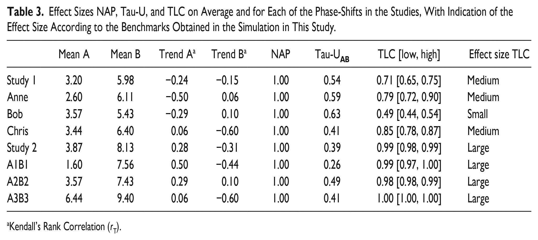
Kendall’s Rank Correlation (r_T).

The QoL of the three participants in study 1 improves between phases. The effect sizes NAP, Tau-U and TLC support the evidence that change in QoL can be attributed to intervention X (average ESs: NAP = 1.00; Tau-U = 0.54; TLC = 0.71; Table 3). Jennifer’s QoL (study 2) improved when the intervention was introduced (A1B1) and decreased when the intervention was withdrawn (B1A2). QoL improved again due to the intervention (A2B2). This pattern occurred again with the second reversal (B2A3 and A3B3). The effect sizes support the evidence of the study for the functional relationship between intervention X and QoL in study 2 as well (average ESs: NAP = 1.00; Tau-U = 0.39; TLC = 0.99; Table 3).

Although the immediacy of the effect is not as clear for each phase shift and there are some positive baseline trends, these two studies with both three demonstrations of the intervention effect point to evidence for the effectiveness of intervention X. NAP, Tau-U, and TLC differ with respect to which study shows more evidence (Table 3). NAP does not discriminate (1.00 = 1.00), Tau-U prefers study 1 (0.54 > 0.39), while TLC prefers study 2 (0.71 < 0.99). This shows that NAP, Tau-U, and TLC discern differently between the effect sizes. Closer inspection can reveal which of the three is most in line with an intuitive understanding based on all relevant aspects of a visual analysis of the data.

Ceiling Effect

In study 1 and 2, NAP clearly suffers from a ceiling effect, while Tau-U and TLC do not. NAP is 1.00 for all comparisons and therefore does not discriminate between the size of effects between the studies. Tau-U and TLC do discriminate between the two studies, albeit in a different order. The different order of effects by TLC and Tau-U occurs because they differ in how they deal with (over)compensating for trend and taking typicality into account. There is some undesirable trend in study 2 (Table 3 shows the upward trend during baselines (r_T = 0.28) and downward trend during intervention phases (r_T = −0.31) in study 2. In study 1 there is no undesirable trend in baseline r_T = −0.24) and less in intervention phase (r_T = −0.15). Therefore, Tau-U is higher in study 1. According to TLC however, there is a large effect in study 2, and a medium effect in study 1.

This is due to the greater level-change in study 2 (8.13−3.87 = 4.26) in comparison to study 1 (5.98−3.20 = 2.78), TLC is higher for study 2.

Correcting for Trend

Looking only at the upper panels of the two studies in Figure 3, the trend differs between the two studies. In the multiple baselines design, Anne’s baseline shows downward trend: her QoL declines over time and an improvement during the intervention phase would break this trend. Study 2 (ABABAB-design) starts with a slightly positive trend: Jennifer’s QoL seems to be improving gradually during the baseline phase, meaning the data shows a positive baseline trend. Even when no intervention was performed, this could hypothetically continue.

Tau-U may overcorrect for trend, as becomes apparent when we look closer in the pairwise comparisons. Although Anne (Tau-U = 0.59; TLC = 0.79) shows less positive trend during baseline than Jennifer’s first baseline A1 (Tau-U = 0.26; TLC = 0.99), the difference in immediacy and amount of level-change might be more important here in determining, which effect is stronger. The large consistent difference between the end of the baseline and the beginning of the intervention in Jennifer’s data (from maximally 3 during baseline to consistently more than 7 during intervention), indicates change while the modest trend that occurs can be relaxed, because of the convincing immediacy of the effect.

Also, when we compare the panel of Bob (Tau-U = 0.63; TLC = 0.49) with the panel of A2B2 (Tau-U = 0.49; TLC = 0.98), just looking at trend might lead to believe the phase-shift of Bob is more convincing. However, the change of QoL is less than 2 points in the case of Bob compared to over 3 in A2B2, while both having rather stable measurements in both phases. To interpret the increase in QoL from A2 to B2 as a consequence of a continued trend, is not plausible and one better ignores the problematic trend here in calculating an effect size after inspecting it in visual analysis.

TLC does not adjust for trend, making it prone to error when problematic trends occur. To detect a problematic trend, we propose an indirect technique that avoids the risk of overcompensation like Tau-U does. To investigate whether trend causes problems in the interpretation of the effect, two TLCs can be calculated from the data using a split-half technique when the design consists of phases with a length of at least five. If there is no trend, the split-half TLCs should be equal. Figure 4 shows situations in which there is no trend and trend: in the upper panel of Figure 4 there is no trend in both phases, because the short term effect (A2B1) does not differ from the long term effect (A1B2). The short term or immediate effect is reflected by TLC_S for the second half of data points during baseline (A₂) and the first half of data points during intervention phase (B₁). The long term effect is reflected by TLC_L for the first half of data points in baseline (A₁) and the second half of data points during intervention (B₂). In the second panel of Figure 4, there is a positive trend in both phases, so the long term difference in level will be much larger, and is reflected by TLC_L > TLC_S.

Figure 4.

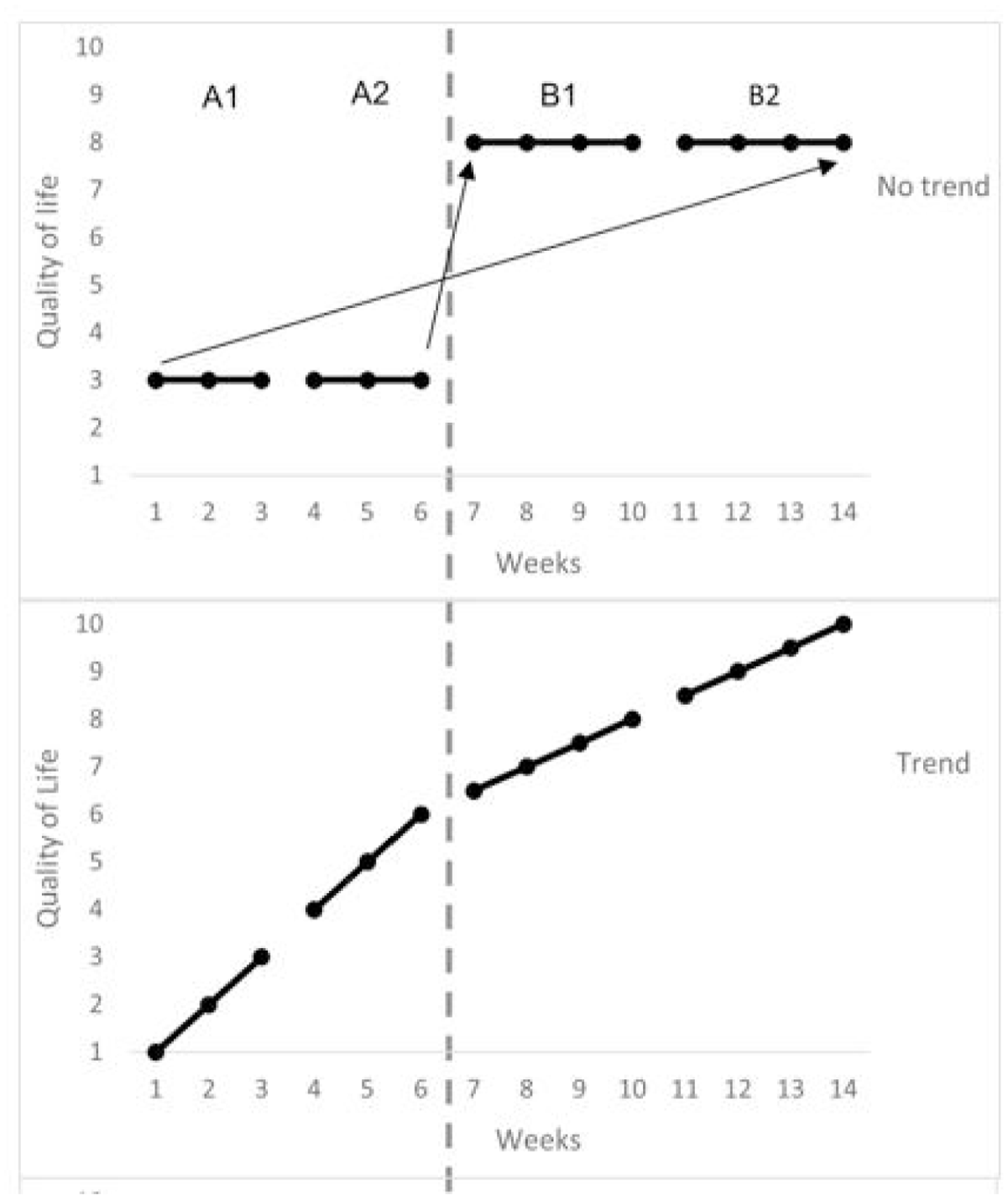
Examples of split-half techniques to detect problematic trend. No indication of trend (TLC_S = TLC_L) in panel 1, indication of trend (TLC_S < TLC_L) in panel 2.

For the A1B1-phaseshift in our example, TLC_L > TLC_S, but there is overlap between the confidence intervals (Table 4). Demonstration of an effect is not doubtful in this phase shift: if this applies to the other replications as well, it is plausible that the change in QoL was caused by the intervention. The calculation of the TLC_S and TLC_L of A1B1 is illustrated in Table 4.

Table 4.

Calculation of TLC_L and TLC_S to Obtain an Indication of Problematic Trend for the First Phase-Shift in the ABAB-Design of Study 2.

Term	Phase	Data	Sum score	Corrected^a sum score	Rounded^b corrected sum score	TLC [CI]
TLC_L	A₁	1 1 2	4	6.67	7	0.97 [0.95, 0.98]
TLC_L	B₂	8 7 7 7 7	36	36	36	0.97 [0.95, 0.98]
TLC_S	A₂	2 1 3	6	10	10	0.99 [0.98, 1.00]
TLC_S	B₁	9 9 7 7 8	40	40	40	0.99 [0.98, 1.00]

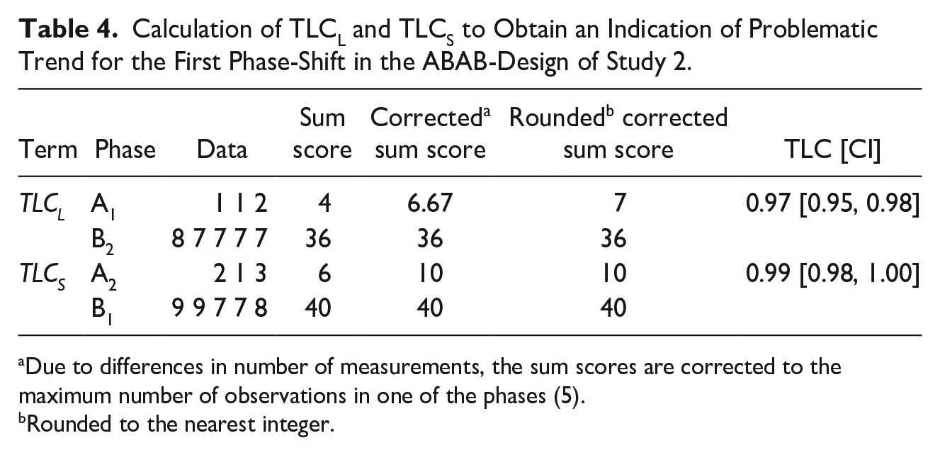
Due to differences in number of measurements, the sum scores are corrected to the maximum number of observations in one of the phases (5).

Rounded to the nearest integer.

Taking Typicality Into Account

Finally, when trend and difference in level between phases are identical, but the baseline value differs between participants, considering typicality of change helps to differentiate between effects. In the bottom panels of Figure 3, the development of Chris and Jennifer’s final replication A3B3 is depicted and shows that Jennifer consistently scores a point more than Chris. NAP (1.00) and Tau-U (0.41) are the same for both. The question remains whether Chris’ replication is as convincing as this phase shift in Jennifer: Jennifer could not have improved much more, because the measurement scale limits this. Her quality of life is almost as good as it can be in A3. Chris’ quality of life though could have been improved more (5.7 during the intervention). The concern here is that an improvement in the mean on a scale of 1 to 10, from 3.4 to (at least) 6.4 is not as typical as an improvement from 6.4 to (at least) 9.4, although the magnitude of difference in level between the phases is the same (3). When the data of Chris and Jennifer’s final replication A3B3 are presented alternatively (Figure 5), where the lowest score at baseline is recoded to 0% (3 for Chris and 6 for Jennifer) and the highest possible value (10 in both cases) would be recoded 100%, the graphs show the typicality of improved quality of life of both. From a typicality point of view, Jennifer’s development should be reflected with a larger effect size. Chris (TLC = 0.85) and Jennifer (TLC = 1.00) are ordered in a way that the change is greater for Jennifer when TLC is used as an effect measure.

Figure 5.

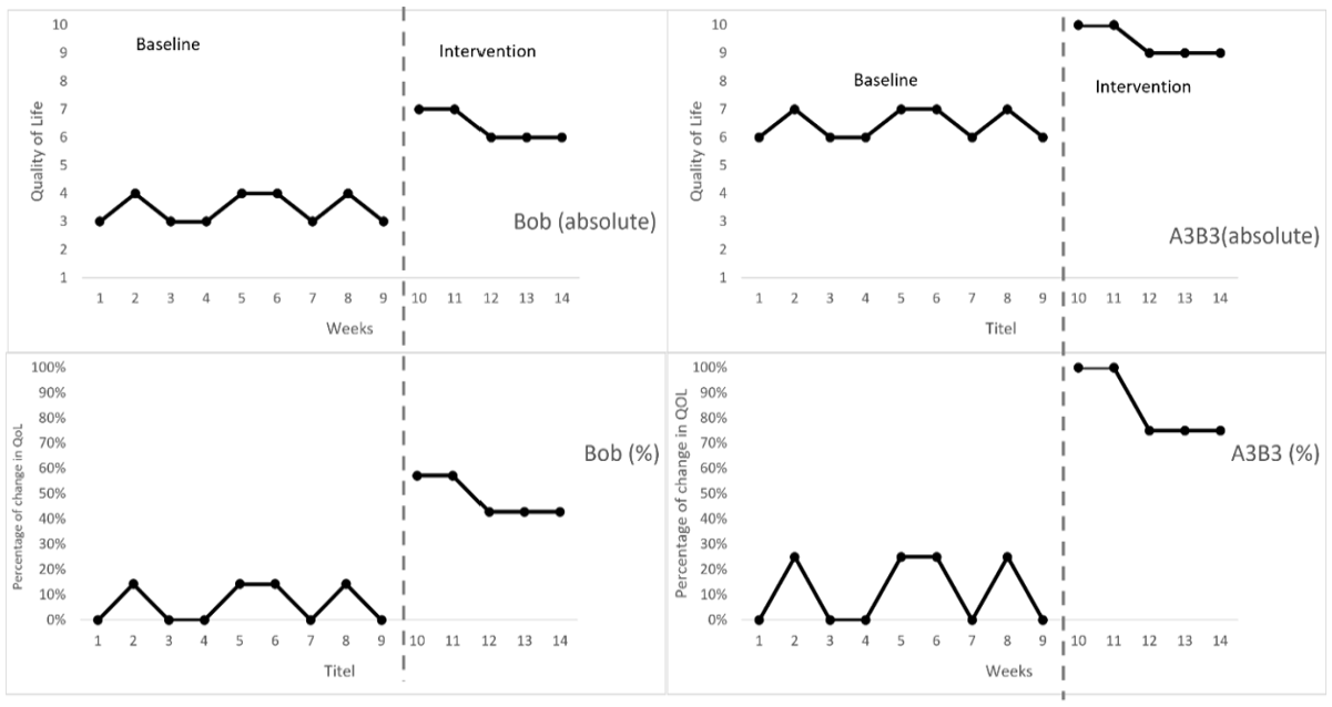
Comparison between Chris and Jennifer’s A3B3-phases, with respect to their percentage of improvement in comparison to their own lowest measured quality of life (bottom two panels): the improvement in the QOL is more typical in Jennifer’s phase-shift.

Some conclusions with respect to which effect is larger might be open to discussion, such as those regarding the typicality of level change, but from visual analysis of Figure 5, ordering the right panels over the left panels, favoring superior level changes over slightly troubling trends during the baseline phase, seems hardly doubtful. For Tau-U, this ranking is entirely different, consistently favoring the phase shifts in the MBD over the ABABAB-design. For NAP, this leads to no ranking at all because all NAPs are maximum due to the ceiling effect. With TLC, the ordering of effects fits the conclusions of the results of visual analysis.

Discussion

In SCR statistical effect sizes are used to formally decide the degree to which an intervention has worked. Conclusions based on visual analyses are sensitive for subjective interpretations, especially when the effects are visually difficult to discern. In a standardized visual analysis six aspects of the data are considered to formulate a decision. Statistical effect sizes must therefore as much as possible be in line with the categories of visual analysis. Violation of assumptions of parametric effect size indices and tests are not uncommon in SCR due to small amount of measurement points. For such situations nonoverlap methods, such as NAP and Tau-U, are recommended. Both indices partly cover the six categories of visual analyses. By not explicitly weighing the size of level-change in the effect size, nonoverlap methods are prone to three restrictions: a ceiling effect, ignoring or overcompensating trend, and not taking into account the typicality of the level-change. In this study, we introduced TLC as a statistical effect size index that can be used in situations where properties of the data in a SCR do not allow the use of parametric alternatives, and a researcher still wants to acquire, besides visual interpretation, formal information about the effect size for each change of conditions in the single case design. Other than NAP and Tau-U, TLC is explicitly computed from level-change: the first of six variables that is taken into consideration in a visual analysis (Kratochwill & Levin, 2010; Ray, 2015).

In SCR, typically the goal is to find or refute evidence for interventions. A ceiling effect or overcompensated trend is not much of a problem as these binary decisions do not often lead to Type I- and Type II-errors when using nonoverlap methods. Tau-U and NAP are sufficient if establishing evidence is the purpose of the study. Also, one could use a parametric alternative as recommended by the WWC (2020). However, if we want to obtain more detailed information about the size of effect of each replication, TLC does not assume normal distribution of the data and weighs in more relevant characteristics of the data, which enables to differentiate more in small data sets.

Limitations and Future Research

There are some limitations to the current study. Benchmarks for small, medium, and large effects have been obtained by simulation but are not yet validated by field data. Also, to calculate TLC, the measurement scale must have an absolute minimum and maximum value, which is not the case for count data. To use TLC for count data, the data should first be recoded into ordinal scale categories. Whether this is always possible and desirable depends on the research situation and the properties of the data.

Several directions for future research of this effect size index are recommended. Firstly, it would be interesting to reanalyze published data with TLC, to see if taking into account typicality of an effect leads to different results and different nuances to the effects that were found. For instance, Parker et al. (2011) found 25% from a convenience sample of published articles using AB designs, yielded a NAP of 1.00. Analyzing this data again with TLC would lead to more differentiated conclusions from this data. The simulations in this study to find typical values of TLC already showed that TLC can discriminate when there is complete nonoverlap between phases.

Secondly, the principle of TLC is quite easy to understand, but calculation can be hard, even in cases with few data. Syntax in SPSS or R are not yet available, but calculation of TLC is possible in Excel for a variety of designs (ABAB, alternate treatment and multiple baseline) by using the available link to the spreadsheets in Supplement 3. The use of TLC is not limited to these designs. TLC can be used in any single case design that has two-phase comparison as the basic unit of analysis. It could be worthwhile to expand the opportunity to calculate TLC to a greater variety of designs.

Also, simulations need to consider the possible influence of the length of phases and the type of measurement scales on benchmarks as well. In addition, TLC should be compared to other effect sizes such as standardized mean difference (Busk & Serlin, 1992), log response ratio (Swann & Pustejovsky, 2018), and d-statistic (Shadish et al., 2014). Also, the relative robustness of TLC to autocorrelation has not yet been clarified, but is an important threat to any effect-measure in the field of SCR (Franklin et al., 1996). Finally, TLC needs to be field-tested to show what results would be generated in practice.

Despite most SCRs are underpowered when insufficient randomization was built into the design (Ferron & Onghena, 1996), in SCR, the goal is usually to find large effects that can hardly be discarded (Kazdin, 2011). The TLC is a distribution free index, which can be applied to any data set that meets the WWC (2020) guidelines, despite that these designs may not have the statistical power to find rather small effects. The WWC guidelines instruct to include three replications in MBDs or Reversal Designs, with at least three data points in each phase to meet standards with reservations, and at least five data points in each phase to meet standards.

Conclusion

This article introduced a non-parametric effect size index TLC for small data in single case research designs. While visual analysis is prone to subjectivity, distributional properties of small data often rule out parametric approaches, and existing nonoverlap methods NAP and Tau-U do have restrictions, TLC gives a standardized indication of the size of an effect between phases in SCR designs with small data. We illustrated with two hypothetical studies that, unlike NAP and Tau-U, TLC differentiates effects more in line with the outcomes of visual analysis. The TLC enables researchers to compare effects between participants and between studies based on typicality, offering a more precise measure of effect than NAP and Tau-U.

Supplemental Material

sj-docx-1-bmo-10.1177_01454455231190741 – Supplemental material for Typicality of Level Change (TLC) as an Additional Effect Measure to NAP and Tau-U in Single Case Research

Supplemental material, sj-docx-1-bmo-10.1177_01454455231190741 for Typicality of Level Change (TLC) as an Additional Effect Measure to NAP and Tau-U in Single Case Research by Willem Landman, Stefan Bogaerts and Marinus Spreen in Behavior Modification

Supplemental Material

sj-docx-2-bmo-10.1177_01454455231190741 – Supplemental material for Typicality of Level Change (TLC) as an Additional Effect Measure to NAP and Tau-U in Single Case Research

Supplemental material, sj-docx-2-bmo-10.1177_01454455231190741 for Typicality of Level Change (TLC) as an Additional Effect Measure to NAP and Tau-U in Single Case Research by Willem Landman, Stefan Bogaerts and Marinus Spreen in Behavior Modification

Supplemental Material

sj-docx-3-bmo-10.1177_01454455231190741 – Supplemental material for Typicality of Level Change (TLC) as an Additional Effect Measure to NAP and Tau-U in Single Case Research

Supplemental material, sj-docx-3-bmo-10.1177_01454455231190741 for Typicality of Level Change (TLC) as an Additional Effect Measure to NAP and Tau-U in Single Case Research by Willem Landman, Stefan Bogaerts and Marinus Spreen in Behavior Modification

Footnotes

Author’ s Note

Stefan Bogaerts is also affiliated to Fivoor, Academy of Research Innovation and Development, Poortugaal, The Netherlands.

Declaration of Conflicting Interests

The author(s) declared no potential conflicts of interest with respect to the research, authorship, and/or publication of this article.

Funding

The author(s) received no financial support for the research, authorship, and/or publication of this article.

ORCID iD

Willem Landman

Supplemental Material

Supplemental material for this article is available online.

Author Biographies

Willem Landman is a PhD candidate at Developmental Psychopathology and Forensic Psychology, Tilburg University, School of Social and Behavioral Sciences, Department of Developmental Psychology, Tilburg, The Netherlands, and teacher in in Social Work, NHL Stenden University of Applied Sciences, Academy of Social Studies, Leeuwarden, The Netherlands.

Stefan Bogaerts is a professor of Developmental Psychopathology and Forensic Psychology, Tilburg University, School of Social and Behavioral Sciences, Department of Developmental Psychology, Tilburg, The Netherlands, and head research & treatment, Fivoor, Academy of Research Innovation and Development, Poortugaal, The Netherlands.

Marinus Spreen, fomer lector Small-n designs and teacher in Social Work, NHL Stenden University of Applied Sciences, Academy of Social Studies, Leeuwarden, The Netherlands.

References

Abrahamsson

Ahlund

Ahrin

Alfonsson

(2018). Video-based CBT-E improves eating patterns in obese patients with eating disorder: A single case multiple baseline study. Journal of Behavior Therapy and Experimental Psychiatry, 61, 104–112. https://doi.org/10.1016/j.jbtep.2018.06.010

Baek

E. K.

Moeyaert

Petit-Bois

Beretvas

S. N.

Van den Noortgate

Ferron

J. M.

(2014). The use of multilevel analysis for integrating single-case experimental design results within a study and across studies. Neuropsychological Rehabilitation: Single-Case Experimental Design Methodology, 24(3–4), 590–606. https://doi.org/10.1080/09602011.2013.835740

Baldwin

V. N.

Powell

(2015). Google calendar: A single case experimental design study of a man with severe memory problems. Neuropsychological Rehabilitation, 25(4), 617–636. https://doi.org/10.1080/09602011.2014.956764

Barlow

D. H.

Nock

M. K.

Hersen

(2009). Single case experimental designs: Strategies for studying behavior for change. Pearson.

Barton

E. E.

Meadan

Fettig

(2019). Comparison of visual analysis, non-overlap methods, and effect sizes in the evaluation of parent implemented functional assessment based interventions. Research in Developmental Disabilities, 85, 31–41. https://doi.org/10.1016/j.ridd.2018.11.001

Brodhead

Kim

Rispoli

Sipila

Bak

(2019). A pilot evaluation of a treatment package to teach social conversation via video-chat. Journal of Autism and Developmental Disorders, 49(8), 3316–3327. https://doi.org/10.1007/s10803-019-04055-4

Brossart

D. F.

Laird

V. C.

Armstrong

T. W.

(2018). Interpreting Kendall’s Tau and Tau-U for single-case experimental designs. Cogent Psychology, 5(1), 1518687. https://doi.org/10.1080/23311908.2018.1518687

Brossart

D. F.

Parker

R. I.

Olson

E. A.

Mahadevan

(2006). The relationship between visual analysis and five statistical analyses in a simple AB single-case research design. Behavior Modification, 30(5), 531–563. https://doi.org/10.1177/0145445503261167

Busk

P. L.

Serlin

R. C.

(1992). Meta-analysis for single-case research. In Kratochwill

T. R.

Levin

J. R.

(Eds.), Single-case research design and analysis (pp. 187–212). Lawrence Erlbaum Associates, Inc.

10.

Collier-Meek

M. A.

Sanetti

L. M. H.

Levin

J. R.

Kratochwill

T. R.

Boyle

A. M.

(2019). Evaluating implementation supports delivered within problem-solving consultation. Journal of School Psychology, 72, 91–111. https://doi.org/10.1016/j.jsp.2018.12.002

11.

Dart

E. H.

Radley

K. C.

(2017). The impact of ordinate scaling on the visual analysis of single-case data. Journal of School Psychology, 63, 105–118. https://doi.org/10.1016/j.jsp.2017.03.008

12.

Davis

J. L.

(2014). Non-overlap analysis for single-case research. In Parker

R. I.

Vannest

K. J.

(Eds.), Single-case intervention research: Methodological and statistical advances (pp. 127–151). American Psychological Association. https://doi.org/10.1037/14376-005

13.

Erhardsson

Alt Murphy

Sunnerhagen

K. S.

(2020). Commercial head-mounted display virtual reality for upper extremity rehabilitation in chronic stroke: A single-case design study. Journal of Neuroengineering and Rehabilitation, 17(1), 154. https://doi.org/10.1186/s12984-020-00788-x

14.

Ferron

Onghena

(1996). The power of randomization tests for single-case phase designs. Journal of Experimental Education, 64, 231–239.

15.

Franklin

R. D.

Gorman

B. S.

Beasley

T. M.

Allison

D. B.

(1996). Graphical display and visual analysis. In Franklin

R. D.

Allison

D. B.

Gorman

B. S.

(Eds.), Design and analysis of single-case research (1st ed., pp. 119–158). Erlbaum.

16.

Gage

N. A.

Lewis

T. J.

(2014). Hierarchical linear modeling meta-analysis of single-subject design research. The Journal of Special Education, 48(1), 3–16. https://doi.org/10.1177/0022466912443894

17.

Hein

Weeland

(2019). Introduction to the special issue. Randomized Controlled Trials (RCTs) in clinical and community settings: Challenges, alternatives and supplementary designs. In Hein

Weeland

(Eds.), New directions for child and adolescent development (Vol. 167, pp. 7–15). Wiley Periodicals, Inc.

18.

Heyvaert

Onghena

(2014). Analysis of single-case data: Randomisation tests for measures of effect size. Neuropsychological Rehabilitation, 24(3–4), 507–527. https://doi.org/10.1080/09602011.2013.818564

19.

Heyvaert

Saenen

Maes

Onghena

(2015). Comparing the percentage of non-overlapping data approach and the hierarchical linear modeling approach for synthesizing single-case studies in autism research. Research in Autism Spectrum Disorders, 11(3), 112–125. https://doi.org/10.1016/j.rasd.2014.12.002

20.

Horner

R. H.

Carr

E. G.

Halle

McGee

Odom

Wolery

(2005). The use of single-subject research to identify evidence-based practice in special education. Exceptional Children, 71(2), 165–179. https://doi.org/10.1177/001440290507100203

21.

Jamieson

Monastra

Gillies

Manolov

Cullen

McGee-Lennon

Brewster

Evans

(2019). The use of a smartwatch as a prompting device for people with acquired brain injury: A single case experimental design study. Neuropsychological Rehabilitation, 29(4), 513–533. https://doi.org/10.1080/09602011.2017.1310658

22.

Kazdin

A. E.

(2011). Single-case research designs. Oxford University Press.

23.

Kratochwill

T. R.

Hitchcock

J. H.

Horner

R. H.

Levin

J. R.

Odom

S. L.

Rindskopf

D. M.

Shadish

W. R.

(2013). Single-case intervention research design standards. Remedial and Special Education, 34(1), 26–38. https://doi.org/10.1177/0741932512452794

24.

Kratochwill

T. R.

Levin

J. R.

(2010). Enhancing the scientific credibility of single-case intervention research. Psychological Methods, 15(2), 124–144. https://doi.org/10.1037/a0017736

25.

Kunze

M. G.

Machalicek

Wei

St Joseph

(2021). Coaching via telehealth: Caregiver-mediated interventions for young children on the waitlist for an autism diagnosis using single-case design. Journal of Clinical Medicine, 10(8), 1654. https://doi.org/10.3390/jcm10081654

26.

Lane

J. D.

Gast

D. L.

(2014). Visual analysis in single case experimental design studies: Brief review and guidelines. Neuropsychological Rehabilitation, 24(3–4), 445–463. https://doi.org/10.1080/09602011.2013.815636

27.

Lenz

A. S.

(2015). Using Single-Case research designs to demonstrate evidence for counseling practices. Journal of Counseling & Development, 93(4), 387–393. https://doi.org/10.1002/jcad.12036

28.

Manolov

Moeyaert

(2017). Recommendations for Choosing Single-Case Data Analytical Techniques. Behavior Therapy, 48(1), 97–114. https://doi.org/10.1016/j.beth.2016.04.008

29.

McGoldrick

Crawford

Evans

J. J.

(2021). MindMate: A single case experimental design study of a reminder system for people with dementia. Neuropsychological Rehabilitation, 31(1), 18–38. https://doi.org/10.1080/09602011.2019.1653936

30.

Odom

L.S.

Barton

E. E.

Reichow

Swaminathan

Pustejovsky

J. E.

(2018). Between-case standardized effect size analysis of single case designs: Examination of the two methods. Research in Developmental Disabilities, 79, 88–96. https://doi.org/10.1016/j.ridd.2018.05.009

31.

Parker

R. I.

Brossart

D. F.

(2003). Evaluating single-case research data: A comparison of seven statistical methods. Behavior Therapy, 34(2), 189–211. https://doi.org/10.1016/S0005-7894(03)80013-8

32.

Parker

R. I.

Vannest

(2009). An improved effect size for single-case research: Nonoverlap of all pairs. Behavior Therapy, 40(4), 357–367. https://doi.org/10.1016/j.beth.2008.10.006

33.

Parker

R. I.

Vannest

K. J.

Davis

J. L.

Sauber

S. B.

(2011). Combining nonoverlap and trend for single-case research: Tau-U. Behavior Therapy, 42(2), 284–299. https://doi.org/10.1016/j.beth.2010.08.006

34.

Rakap

(2015). Effect sizes as result interpretation aids in single-subject experimental research: Description and application of four nonoverlap methods. British Journal of Special Education, 42(1), 11–33. https://doi.org/10.1111/1467-8578.12091

35.

Ray

D. C.

(2015). Single-Case research design and analysis: Counseling applications. Journal of Counseling & Development, 93(4), 394–402. https://doi.org/10.1002/jcad.12037

36.

Rindskopf

(2014a). Bayesian analysis of data from single case designs. Neuropsychological Rehabilitation: Single-Case Experimental Design Method-ology, 24(3–4), 572–589. https://doi.org/10.1080/09602011.2013.866903

37.

Rindskopf

(2014b). Nonlinear Bayesian analysis for single case designs. Journal of School Psychology, 52(2), 179–189. https://doi.org/10.1016/j.jsp.2013.12.003

38.

Rouanet

Bernard

J. M.

Bert

M. C.

Lecoutre

M. P.

Le Roux

(2000). New ways in statistical methodology: From significance tests to Bayesian inference (2nd ed.). Peter Lang AG.

39.

Scruggs

T. E.

Mastropieri

M. A.

Casto

(1987). The quantitative synthesis of single-subject research: Methodology and validation. RASE: Remedial & Special Education, 8(2), 24–33. https://doi.org/10.1177/074193258700800206

40.

Shadish

W. R.

Hedges

L. V.

Pustejovsky

J. E.

(2014). Analysis and meta-analysis of single-case designs with a standardized mean difference statistic: A primer and applications. Journal of School Psychology, 52(2), 123. https://doi.org/10.1016/j.jsp.2013.11.005

41.

Snijders

T. A. B.

Borgatti

S. P.

(1999). Non-parametric standard errors and tests for network statistics. Connections, 2, 61–70. https://www.stats.ox.ac.uk/~snijders/Snijders_Borgatti.pdf

42.

Spauwen

Ter Mors

van Harten

Domensino

Ponds

van Heugten

(2020). Efficacy and safety of amantadine as a treatment for apathy after brain injury: Two single-case experimental design studies. Neuropsychological Rehabilitation, 32(6), 872–896. https://doi.org/10.1080/09602011.2020.1842214

43.

Spreen

(1992). Rare Populations, Hidden Populations, and Link-Tracing Designs: What and Why? Bulletin of Sociological Methodology/Bulletin de Méthodologie Sociologique, 36(1), 34–58. https://doi.org/10.1177/075910639203600103

44.

Spreen

Timmerman

M. E.

Ter Horst

Schuringa

(2010). Formalizing clinical decisions in individual treatments: Some first steps. Journal of Forensic Psychology Practice, 10(4), 285–299. https://doi.org/10.1080/15228932.2010.481233

45.

Swaminathan

Rogers

H. J.

Horner

R. H.

Sugai

Smolkowski

(2014). Regression models and effect size measures for single case designs. Neuropsychological Rehabilitation: Single-Case Experimental Design Method-ology, 24(3–4), 554–571. https://doi.org/10.1080/09602011.2014.887586

46.

Swann

D. M.

Pustejovsky

J. E.

(2018). A gradual effects model for single-case designs. Multivariate Behavioral Research, 53(4), 574–593. https://doi.org/10.1080/00273171.2018.1466681

47.

Tanious

De Kumar

Michiels

Van den Noortgate

Onghena

(2020). Assessing consistency in single-case A-B-A-B phase designs. Behavior Modification, 44(4), 518–551. https://doi.org/10.1177/0145445519837726

48.

Tarlow

K. R.

(2017). An improved rank correlation effect size statistic for single-case designs: Baseline corrected tau. Behavior Modification, 41(4), 427–467. https://doi.org/10.1177/0145445516676750

49.

Vannest

K. J.

Ninci

(2015). Evaluating intervention effects in Single-Case research designs. Journal of Counseling & Development, 93(4), 403–411. https://doi.org/10.1002/jcad.12038

50.

Wong

S. E.

(2010). Single-case evaluation designs for practitioners. Journal of Social Service Research, 36(3), 248–259. https://doi.org/10.1080/01488371003707654

51.

What Works Clearinghouse. (2020). Chapter 4. What works clearinghouse procedures handbook (Version 4.1). U.S. Department of Education, Institute of Education Sciences, National Center for Education Evaluation and Regional Assistance. https://ies.ed.gov/ncee/wwc/handbooks

52.

Yaffee

R. A.

McGee

(2000). Introduction to time series analysis and forecasting. Academic Press.

Supplementary Material

Please find the following supplemental material available below.

For Open Access articles published under a Creative Commons License, all supplemental material carries the same license as the article it is associated with.

For non-Open Access articles published, all supplemental material carries a non-exclusive license, and permission requests for re-use of supplemental material or any part of supplemental material shall be sent directly to the copyright owner as specified in the copyright notice associated with the article.

0.00 MB

0.02 MB

0.01 MB