
Abstract
Due to the rapid adoption of renewable energy sources and the increasing complexity of residential electricity consumption, there is a growing need for intelligent, scalable, and context-aware energy management systems in smart homes. This paper presents an artificial intelligence (AI)-based model that integrates high-resolution household power forecasting with dynamic demand response (DR) simulations to optimize energy consumption, enhance grid stability, and support sustainable energy transitions. Using the publicly available UCI Smart Home Energy dataset, a seven-step framework was implemented, including data preprocessing, exploratory data analysis (EDA), feature engineering, and the development of various predictive models—linear regression (LR), random forest regressor (RFR), support vector regression (SVR), k-nearest neighbors (k-NN), and long short-term memory (LSTM) neural networks. Each model was evaluated under seven DR strategies to capture temporal dependencies and nonlinear load behaviors: Peak Clipping, Valley Filling, Load Shifting, Load Leveling, Time-of-Use (ToU) Optimization, Price-Based Control, and Behavioral DR. Model performance was assessed using the mean absolute error (MAE), root mean squared error (RMSE), and the coefficient of determination (R²). Results revealed that the LSTM model achieved the highest accuracy, with the lowest MAE (18.95 Wh), lowest RMSE (24.83 Wh), and highest R² (0.94) under the Price-Based DR strategy. Random forest emerged as the most effective traditional model, yielding an MAE of 25.13 Wh and R² of 0.89, particularly for Behavioral and ToU-based DR strategies. The SVR and k-NN models provided moderate accuracy, while LR performed poorly, underscoring its limitation in modeling nonlinear and dynamic energy patterns. DR simulations indicated that Price-Based, Behavioral, and ToU Optimization strategies achieved the best alignment between household loads and grid requirements while maintaining user flexibility. Visualization tools such as heatmaps, grouped bar plots, and R² comparisons further confirmed the superior temporal modeling capability of deep learning (DL) methods. Overall, the proposed framework offers a scalable and interpretable AI-driven platform that integrates load forecasting with DR evaluation, demonstrating that DL—particularly LSTM—can substantially enhance forecasting accuracy, enable smarter DR programs, and promote sustainable energy management in smart homes.
Keywords
Introduction
Energy sector transformation and demand challenges
The global energy sector is undergoing a profound transformation driven by the urgent need to mitigate climate change, rising electricity demand, and the large-scale integration of renewable energy sources. According to the International Energy Agency, global energy consumption is projected to increase by nearly 50% by 2050, with most of this growth occurring in developing economies (Bouckaert et al., 2021). Traditional power grids, originally designed for unidirectional power flow from centralized plants to passive consumers, are now challenged by the bidirectional flows and variability introduced by modern renewable generation. Intermittent sources such as solar and wind create significant supply fluctuations that often exceed demand variations, complicating real-time grid management. Consequently, advanced strategies such as demand response (DR) programs are increasingly being adopted to dynamically adjust electricity consumption in response to grid conditions (AbdelRaouf et al., 2024).
DR in modern grids
DR has emerged as a cornerstone of modern energy management, redefining the traditional demand–supply paradigm by enabling consumption patterns to influence electricity generation rather than merely respond to it. The US Department of Energy defines DR as programs designed to reduce or shift electricity usage during peak periods through time-based pricing or incentive mechanisms (Cappers et al., 2010). Effective implementation of DR can alleviate peak demand, enhance grid reliability, lower operational costs, and reduce greenhouse gas emissions. However, conventional DR schemes are often manual and rule-based, making them slow to adapt and incapable of capturing the numerous dynamic factors that influence energy consumption. To overcome these limitations, data-driven and intelligent DR approaches have been developed to provide faster, adaptive, and more efficient energy management solutions.
Artificial intelligence and machine learning in energy management
Machine learning (ML) and artificial intelligence (AI) have significantly enhanced the ability to process complex energy data with greater precision and accuracy. In particular, ML techniques are highly effective in identifying patterns and generating reliable predictions from large-scale energy datasets (Kaur et al., 2020). A wide range of ML models has been applied to energy forecasting and optimization. Ensemble learning methods, such as random forests (RFs) and Gradient Boosting Machines, demonstrate strong predictive capabilities by combining the outputs of multiple decision trees (Ardabili et al., 2022).
Researchers have demonstrated that long short-term memory (LSTM) networks perform exceptionally well in modeling sequential energy data. Real-time optimization of energy systems has also been advanced through reinforcement learning techniques (Yu et al., 2021). Despite these developments, several challenges persist. ML models often function as “black boxes,” making their decision-making processes difficult to interpret. They also demand large volumes of high-quality data and substantial computational resources. Moreover, many state-of-the-art algorithms remain proprietary, limiting their accessibility and adoption, particularly in highly regulated sectors.
Modern DR strategies
Modern DR strategies generally fall into three categories that enhance grid load management. In Peak Clipping, electricity consumption is reduced during periods of highest demand—for example, by cycling air-conditioning or heating systems to limit peak loads. In Valley Filling, loads are increased during off-peak periods, such as operating energy-intensive processes at night when the grid can more easily accommodate additional demand. The most adaptive approach, Load Shifting, involves transferring consumption to low-demand periods by utilizing energy storage, such as storing thermal energy for later use. All these strategies rely on accurate forecasting and intelligent control, areas where ML techniques provide a significant advantage (Philipo et al., 2022). Through high-accuracy predictions and advanced optimization algorithms, AI-driven DR systems can automatically determine and implement the most efficient load adjustments for varying conditions, continuously refining their actions as grid dynamics evolve.
Challenges in implementing AI-driven DR
Deploying AI-powered DR systems at scale presents several practical challenges. First, they require timely and reliable data streams; however, collecting, storing, and managing the vast datasets needed to train and operate complex ML models remains nontrivial. Second, customer participation is crucial—users are more likely to engage in automated DR programs when they trust the system's decisions and perceive tangible benefits. Third, existing regulations and market frameworks often need revision to accommodate autonomous DR operations while ensuring fairness and system stability. Cybersecurity is another major concern, as fully automated, internet-connected DR systems introduce new vulnerabilities and require robust defenses against data manipulation or cyberattacks. Finally, real-time control of large-scale DR remains technically demanding, motivating the use of edge computing and distributed algorithms to minimize latency and enhance system resilience (Pereira et al., 2024). Given the interdependence of these factors, the successful deployment of AI-driven DR requires a holistic approach that simultaneously addresses technical, human, and regulatory dimensions.
Research objectives and approach
This research seeks to address the major limitations of existing energy forecasting models and DR schemes to enhance the overall effectiveness of AI-driven energy management. The primary objectives are to develop and evaluate a range of ML and deep learning (DL) models for energy-use prediction, simulate DR strategies—specifically Peak Clipping, Valley Filling, and Load Shifting—and assess their effectiveness using explainability tools and performance metrics. The proposed approach compares conventional predictive methods with advanced ML techniques and introduces a unified framework for measuring DR performance. Practically, the study quantifies potential energy savings and identifies key factors—such as weather conditions and occupancy patterns—that most strongly influence building energy consumption. It also examines how model accuracy correlates with DR success, presenting results in a manner easily interpretable by facility managers. These findings provide valuable insights for utility operators, regulators, researchers, and end users, forming a data-driven basis for more adaptive and responsive energy systems. Moreover, the integrated framework developed herein establishes a consistent methodology for evaluating DR outcomes and clearly demonstrates the potential of AI-driven DR. By combining robust data analytics with real-time adaptability, this work lays a foundation for energy systems that are more reliable, sustainable, and efficient.
Data and methodology
To conduct this research, a publicly available dataset from the UCI ML Repository was utilized. It includes both environmental parameters and appliance-level energy consumption records for residential buildings. The dataset underwent comprehensive preprocessing and feature engineering to prepare it for predictive modeling. An initial exploratory analysis was carried out to examine the data characteristics and guide feature selection. Multiple predictive approaches—ranging from baseline statistical models to advanced ML algorithms—were trained and evaluated through cross-validation using several performance metrics. Model hyperparameters were systematically optimized to enhance predictive accuracy. Finally, the most promising models were applied in simulation studies of three DR strategies—Peak Clipping, Valley Filling, and Load Shifting—under diverse demand scenarios to assess their practical performance (Tahir et al., 2024; Yousaf et al., 2022, 2023, 2025).
Literature review
Recent advances in AI and ML have revolutionized energy forecasting and demand-side management. High-precision short-term load forecasting has been achieved through self-adaptive evolutionary neural networks capable of capturing nonlinear temporal dependencies (Abbas et al., 2025). Advanced LSTM architectures have enhanced accuracy and stability in electricity-imbalance forecasting under stochastic grid conditions (Blinov et al., 2025). ML-based clustering of residential load profiles supports targeted and effective DR implementation (Michalakopoulos et al., 2024). Hybrid ML architectures for grid-connected microgrids with multiple distributed sources outperform conventional time-series approaches in complex networks (Singh et al., 2024a, 2024b). Reviews of AI-empowered energy-consumption methods identify three pillars—load forecasting, anomaly detection, and DR—through which data-driven intelligence improves the reliability and sustainability (Wang et al., 2024).
Optimization-driven DR strategies have progressed rapidly: price-elastic DR coupled with greedy rat-swarm optimization yields superior economic and environmental outcomes by exploiting flexible demand under variable tariffs (Singh et al., 2025a, 2025b, 2025c, 2025d), while coordinated multi-microgrid systems integrating renewables strengthen grid resilience and renewable utilization through adaptive DR algorithms (Pramila et al., 2025). Comprehensive smart residential demand-side management (DSM) frameworks that integrate electric vehicles (EVs) and advanced optimization provide unified control for household energy and peak-load reduction (Panda et al., 2025). Decentralized blockchain-enabled multiagent deep-reinforcement-learning frameworks enable secure, autonomous, real-time DR in renewable grids (Singh et al., 2025a, 2025b, 2025c, 2025d), and DL-based DR mechanisms improve short-term renewable-microgrid operation by learning temporal dependencies (Gharehveran et al., 2024). Blockchain-consortium frameworks enhance interoperability and cybersecurity across DR platforms (Singh et al., 2025a, 2025b, 2025c, 2025d), and hybrid demand-side policies balance economic efficiency with emission control in microgrid management (Singh et al., 2025a, 2025b, 2025c, 2025d). Multiobjective peer-to-peer DR schemes further extend these ideas through network-aware energy sharing and distributed optimization (Tiwari et al., 2024).
AI is increasingly central to mobility-driven DR. AI-integrated blockchain coordination optimizes load balancing in EV-charging networks via predictive scheduling aligned with grid conditions (Singh et al., 2024a, 2024b). Nature-inspired enhanced-cheetah optimization algorithms improve dynamic economic dispatch with renewable participation (Nagarajan et al., 2024), and resilient virtual-power-plant cost optimization incorporates uncertainty modeling for distributed-energy systems under extreme events (Suresh et al., 2025). ML-based real-time energy-management frameworks enhance adaptive load balancing in smart grids (Udo et al., 2024), while cheetah-optimization-based scheduling offers scalable management of appliances and distributed energy resources across residential and industrial sectors (Thirumalai et al., 2025). Integrating hyper-local weather prediction refines DR timing and reduces peak demand (Shaikh et al., 2025), and renewable microgrids with vehicle-to-grid capability demonstrate feasible decentralized DR for smart-village applications (Nadimuthu et al., 2024). Real-time distribution-system scheduling using the crow-search algorithm enhances power allocation and microgrid performance (Selvaraj et al., 2024), while iterative map-based self-adaptive crystal-structure and chaotic sine–cosine algorithms provide efficient multi-objective energy management for EV-integrated hybrid microgrids (Karthik et al., 2024; Rajagopalan et al., 2024).
From a policy and implementation perspective, DSM and market-design reviews emphasize aligning DR mechanisms with flexibility markets to accelerate renewable integration (Panda et al., 2023), and earlier analyses highlight the need for hybrid AI frameworks and robust optimization to ensure scalable residential DSM (Panda et al., 2022). Advanced genetic-algorithm schedulers that jointly consider solar-load forecasting, battery degradation, and DR dynamics achieve balanced techno-economic outcomes (Witharama et al., 2024). EV-centric DSM surveys map strategies, modeling gaps, and operational challenges for mobility-integrated grids (Mohanty et al., 2022). Finally, explainable-AI ensemble clustering for load profiling underscores that interpretability and transparency are prerequisites for trustworthy and large-scale DR deployment (Sarmas et al., 2024).
Advances in energy demand forecasting
Recent progress in ML has led to a significantly more precise forecast of energy use compared to traditional statistical methods, as seen in the work of Antonopoulos et al. (Antonopoulos et al., 2021). Developed a detailed data-driven model based on findings of a large-scale residential smart grid project. Their model, which combines data on time, ecology, and behavior, has made a considerable contribution to the accuracy of predictions and provided valuable information on how consumers react to changes in energy demand. In an overview of the studies on demand-side response, Antonopoulos et al. (2020) presented a comprehensive review of emerging approaches and key advancements in the field. Likewise, it has illustrated the evolving nature of DR through AI and ML-based methods. The reinforcement learning and hybrid predictive models were found to be among the most effective means of controlling energy consumption in real time. It also highlighted that to implement these advanced methods in practice, there should be a clear explanation of the algorithm choices and a high level of protection against cyberattacks to establish trust and security in DR programs.
Notably, common DR operational strategies, such as peak clipping, valley filling, and load shifting, all depend on accurate forecasts and intelligent control capabilities that modern ML methods can effectively provide.
Enhancing predictive accuracy through context and DL
Other studies have explored how incorporating contextual information can further improve ML-based energy predictions. Sari et al. (2023) investigated multiple ML techniques applied to a diverse set of building energy datasets. Their study shows that when temporal and environmental contexts, such as the hour of the day or prevailing weather, are integrated into model design, prediction accuracy improves substantially. This result supports the theoretical view that energy consumption is a behavioral and environmental phenomenon, not merely a technical one. In a similar vein, Wan and Chen investigated the application of DL architectures, specifically those based on convolutional neural networks and attention mechanisms (Wan et al., 2023). Their model captures spatial and temporal dependencies that traditional recurrent networks overlook, giving it the capacity to represent subtle fluctuations in building demand. The work demonstrates how neural attention mechanisms can guide the model toward relevant signals, such as temperature shifts or operational schedules, without requiring human-defined feature hierarchies. Moreover, effective features can help mitigate problems caused by limited data in commercial buildings.
ML in dynamic DR control
The application of DR control strategies in practice is also being transformed by ML. AI-powered solutions enable dynamic adjustments to building systems (e.g. heating, ventilation, air conditioning cycles), resulting in significant reductions in peak demand compared to conventional rule-based control systems. For example, deep reinforcement learning has been integrated with microgrid operations, where adaptive controls are developed through deep reinforcement learning to model operations that coordinate distributed generation, battery storage, and variable loads, thereby matching supply and demand in real time (Sang et al., 2022). Likewise, it has been proven by multiagent learning methods that distributed collaboration among buildings or grid nodes can increase the overall building energy stability and efficiency (Jung et al., 2025). Researchers in the field of human behavioral aspects are also incorporating control strategies. As an example, the E2District framework introduces psychological, cultural, and motivational factors in DR management, as building occupants are regarded as active decision-makers who have an impact on system results (Blanke et al., 2017). These papers suggest that even intelligent control should not focus solely on maximizing technical performance, but also on ensuring user interest and confidence. With increased control over energy consumption being left to algorithms, it is necessary to make their decisions transparent and understandable. Here, explainable artificial intelligence (XAI) is being increasingly recognized as a necessity to ensure that energy management interventions can be understood and are aligned with both technical goals and human expectations.
Explainable and secure AI in energy systems
Table 1 provides a summary of some major works that demonstrate the implementation of explainable AI, ML, and reinforcement learning in various energy contexts, including building energy prediction, microgrid optimization, and cybersecurity. It also presents a summary of the key contributions of each work, identifies research gaps, and provides a direction for continuing studies in the field of AI-driven DR and advanced energy management systems.
Comparative overview of explainable artificial intelligence (XAI), cybersecurity, and demand response (DR) in energy systems.
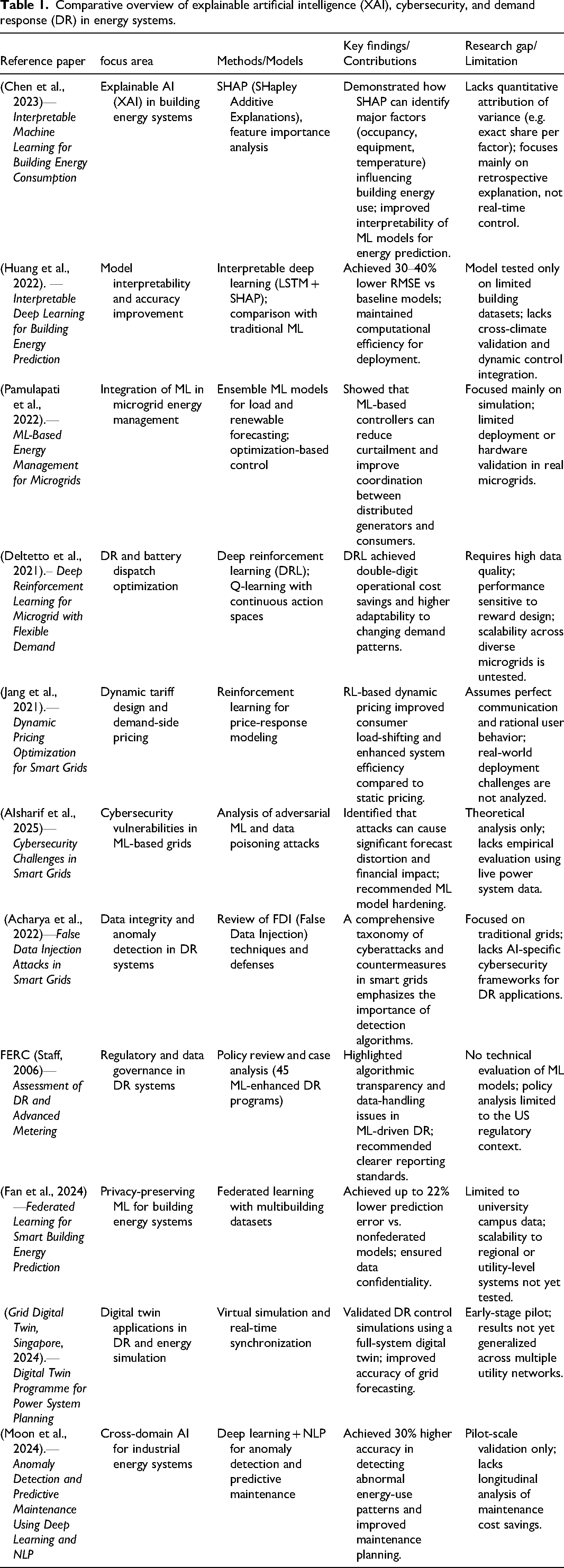
Table 1 shows clear progress in applying ML to forecasting, control, and pricing; however, it also reveals gaps that limit its broad deployment. Many models do not generalize well across different building types or operating contexts, which weakens their responsiveness to diverse occupant behaviors and envelope characteristics. Methods that add interpretability still face a tension with speed and accuracy under operational constraints, so operators need explanations that do not slow down decisions in the field. Cybersecurity and privacy remain weak points for automated DR, with small utilities exposed to data tampering, theft, and weak monitoring. Governance is uneven, since several frameworks focus on prediction or on isolated control functions rather than end-to-end coordination that reflects user needs, market rules, and rare events. Our work addresses these gaps by combining robust forecasting with scenario-tested DR logic, utilizing explainable methods to reveal the drivers of control actions, and incorporating fundamental security and data-handling practices into the pipeline. This approach aims to increase trust, enhance adoption, and deliver measurable savings while facilitating a transition to lower-carbon operations.
Methodology
The approach in this study aims to predict household electricity consumption and examine how various methods to influence demand can alter it, utilizing ML and DL models. Figure 1 illustrates the composition of the entire process into seven well-structured sections. The first step is to preprocess the data by removing inconsistencies and adding or improving new variables to achieve better results in the model. Following this, exploratory data analysis (EDA) is performed to investigate key trends, and data on missing value treatment and anomaly detection measures are implemented to maintain the integrity of the data. Some of the most popular algorithms used in this stage include linear regression (LR), random forest regressor (RFR), support vector regressor (SVR), K-nearest neighbors (K-NNs), and LSTM. Every model will undergo a thoroughly taught and checked training system.
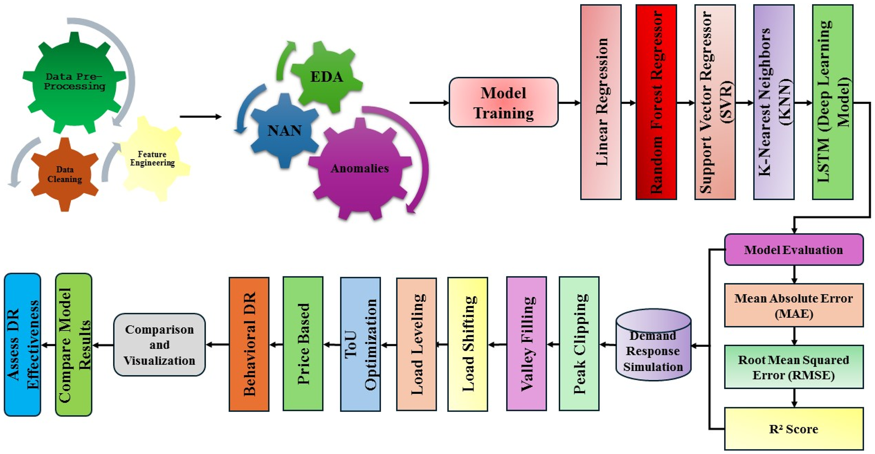
Flowchart of methodology.
Trained models are evaluated by the use of standard performance measurement methods, including the mean absolute error (MAE), root mean squared error (RMSE), and the R² score. They enable evaluating the ability of a model to function in new conditions and comparing it to other algorithms. Demand-side strategies are assessed based on the simulation of the standard types of DR programs. The former is referred to as peak clipping, which saves energy consumption at the peak of demand by delaying or reducing certain activities. The second is Valley Filling, which encourages the use of energy during off-peak periods on the grid, thus maximizing its use. Through Load Shifting, you alternate the hours of the day when you use electrical appliances, thereby consuming the entire amount of electricity you had planned, but at a different time when the power supply is in demand. All these strategies are researched in deeper detail with the assistance of Time-of-Use (ToU) optimization, pricing programs and behavioral change approaches. By these subcategories, we can analyze the effect of price and user activity on energy consumption. The end of the methodology requires checking whether the DR strategies were effective by comparing the model results before and after DR was applied. The techniques make it easy to compare the results and judge whether the improvements to grid stability, peak demand, and energy efficiency do not disrupt the comfort of building occupants.
Data preprocessing
To ensure the reliability and accuracy of the developed models for forecasting household energy consumption, data preprocessing was a crucial initial stage of this research. When the first dataset was received from UCI's smart home energy records, it encountered issues such as missing data, inconsistent values, and errors from sensor generators. Initially, we addressed missing information through forward fill and interpolation. Afterward, we removed any replicated or duplicated entries in the spreadsheet to maintain the integrity of the data. Then, steps were taken to engineer the data and find useful information in it. The timestamps were broken into hour, day, and weekend variables to catch the daily and weekly trends in usage. Factors such as temperature and humidity were included and converted into features called apparent temperature and discomfort index, which show their effect on the usage of HVAC systems and appliances. In addition, categorical variables were transformed using the right method so they would work properly with the model. After that, all numerical features were scaled using Min–Max scaling, ensuring their values remained similar, which made training the model more efficient. With the data passing through this thorough pipeline, the models were able to process it. They had plenty of useful info, helping them capture the detailed tendencies in residential energy use across different times and settings. Here, EDA was conducted to understand the energy consumption pattern and support the selection of features and creation of models. Once the data was cleaned, statistical summaries, plots, and correlation analysis were performed to identify hidden relationships between energy use and factors such as temperature, humidity, time, and the items being used. Initially, we represented energy use in a line plot with seasonal decomposition, which enabled us to observe when and how much energy was being used on a daily, weekly, and seasonal basis. Histograms and boxplots illustrate the distribution of data and the degree of asymmetry, particularly in features such as appliance usage, the number of lights on, and environment-related factors. They pointed out some values that varied significantly from the standard Normal distribution and had to be adjusted before modeling was performed.
Exploratory data analysis
Here, EDA was conducted to understand the energy consumption pattern and support the selection of features and creation of models. Once the data was cleaned, statistical summaries, plots, and correlation analysis were performed to identify hidden relationships between energy use and factors such as temperature, humidity, time, and the items being used. Initially, we represented energy use in a line plot with seasonal decomposition, which enabled us to observe when and how much energy was being used on a daily, weekly, and seasonal basis. Histograms and boxplots illustrate the distribution of data and the degree of asymmetry, particularly in features such as appliance usage, the number of lights on, and environment-related factors. They pointed out some values that varied strongly from the standard Normal distribution and had to be changed before modeling was done. We also applied Pearson correlation tests to determine the extent to which the input features correlated with the target variable (appliance energy consumption). Rooks’ analysis revealed that temperature, humidity, and time were moderately or strongly associated with the results, indicating that they should remain in the model. It was also verified that none of the input features were highly similar to other features, thereby preventing issues with model training. All in all, by completing the EDA phase, we were able to identify the strongest predictors, detect any unusual activity in the data, and observe how energy is utilized in different environments. They helped determine the main features and make the models more valuable afterward.
Handling missing values and anomalies
The dataset was further improved by addressing missing values and anomalies, ensuring the data remained accurate and the model performed more effectively. The main cause of missing values in this research was when certain sensors in the house's environment or appliances malfunctioned, or when log files were corrupted. Short-range gaps were partly eliminated using forward fill interpolation, and individual missing points were filled with the help of mean imputation to keep the time series unchanged. Along with some values missing from the data, the dataset also contained unexpected spikes or drops in energy that occurred without any apparent reason. Both z-scores and visual inspection of charts were used to identify the unusual instances. An observation that falls outside of three standard deviations of the mean was identified as an outlier. Sometimes these problems were handled by smoothing the data locally, and when the data could not be properly fixed, it was discarded. This step was crucial, as missing values and outliers can interfere with the training of regression and ML models, resulting in poor-quality results with numerous errors. Through targeted error detection and proper data imputation, noise and unclear information were removed, making the data suitable and accurate for both learning and DR simulation.
Model training
At this point, a blend of classic ML and advanced DL models was employed to predict household energy consumption, utilizing the features engineered earlier. Through this method of data analysis, it has been established which algorithms can best represent the wide and dynamic patterns frequently observed in residential electricity usage. LR is simple to understand and calculate, hence it has been used as the preferred baseline model. Additionally, the RF ensemble's RFR was chosen due to its ability to identify relationships and dependencies in the data, including nonlinear ones. The SVR was selected due to its benefits in regression tasks involving a large number of variables. Simultaneously, k-NN was chosen to fit the instances of similar data. A LSTM network was employed to manage data dependencies promptly, as it can identify the existence of long-term relationships in time series data. In each model, the training set was refined and enhanced with beneficial factors, such as temperature, humidity, hour, and the history of energy consumption. Classical models were developed using Scikit-learn, whereas TensorFlow and Keras were used to create an LSTM model. To enhance the stability of the models, cross-validation was conducted five times during training, allowing the outcomes to be applied to different sections of the data. Additionally, grid searching or hand-tuning of hyperparameters was also performed based on the outcomes achieved using validation. With this thorough training, each model could be compared fairly and solidly. The study demonstrated that DL is effective for dependent data, but traditional models remain useful when it is crucial for forecasting results to be clear and straightforward.
Model evaluation
Once each model was built, it was thoroughly tested to assess its ability to predict household energy use. To reach this aim, the performance of the regression was evaluated with three basic metrics: MAE, RMSE, and R² score. The MAE calculated the typical error size, whereas RMSE noticed larger errors since it was based on the squared version. With R², we can assess how well the model aligns with the different values in the target variable, thereby gaining a deeper understanding of the model's fit. The calculations were performed on a different set to ensure an unbiased assessment. According to the results, LR and k-NN were not very successful in capturing the changes in the data over time and its complex structure. To sum up, models like RF, based on trees, and SVR proved to be more accurate, as they generalize better to new, unseen instances of data. Due to its effective approach to sequential and time-based dependencies, LSTM outperformed other models in most aspects. During the evaluation phase, the right model was selected, and this stage also served as the basis for comparing results from the DR simulations later. The research ensured that all subsequent DR strategy assessments were based on predictable results by identifying the strengths and weaknesses of each model.
DR simulation
During the sixth step of the study, possible effects of DR strategies on residential electricity consumption were evaluated. Having used the most promising models to predict based on the last step, namely LSTM and RF, the predicted energy consumption was analyzed when considering the three large categories of virtual DR: Peak Clipping, Valley Filling, and Load Shifting. The reasons behind these measures are the need to make the system efficient and balance its power consumption by regulating it based on what the grid requires and the time of day. During periods of peak power demand, Peak Clipping attempts to reduce energy consumption by switching off or postponing the operation of certain appliances in the home. Valley Filling, in the meantime, attempts to maximize its energy consumption on demand, typically by promoting the use of large machines when the power grid is not overloaded. One way to conserve energy by automating or modifying user actions is to shift some loads during busy periods to quieter periods. Three simulation methods, including Time of Use optimization, price-based response, and behavioral response model, were employed to investigate the impact on the load curve resulting from charging electricity at various times of the day and consumer behavior. To develop the simulation results, the predicted energy usage was also varied based on the established DR guidelines, and the effect of this variation on power demand was monitored. Under this option, it was feasible to evaluate the effectiveness of every strategy that contributed to minimizing peak consumption, improving grid efficiency, and promoting environmentally friendly power consumption at households. The simulation data formed the primary foundation of the final analysis and graphics.
Comparative analysis and visualization
The final section of the technique involved a critical comparison of the forecasting models and the simulated DR models. The purpose of this section was to quantify the performance of each algorithm, and the level of energy savings achieved through DR measures. The electric load was analyzed by comparing the predicted load against the actual loads after every DR technique, including Peak Clipping, Valley Filling, and Load Shifting, as well as response models such as Time of Use pricing, reward schemes, and behavioral change incentives. To facilitate the assessment, various visualization tools were applied. Load shifts were easily observed, and a decrease in peak readings was evident, as line plots showed the use of energy before the deployment of DR. Charts displaying the values of the MAE, RMSE, and R² statistics for all models were created to highlight any differences between them. With these graphs, I was able to determine which trading approaches performed best under different market conditions. Through an analysis of the results, the study identified the most effective methods for stabilizing the grid and conserving energy. Demonstrating the accuracy, complexity, and practicality of the approaches helped determine which AI-based DR methods will be most useful in homes.
Results and discussion
Exploratory data analysis
To reveal the peculiarities of and trends in residential energy consumption, an exploratory analysis was performed on the UCI smart home energy dataset. This dataset comprises 19,735 rows and 29 columns, representing temperature, humidity, and power consumption of various appliances. Figure 2 demonstrates a time series plot of the energy consumption of the appliances throughout the dataset. Consumption values are highly variable, and they can sometimes exceed 1000 Wh. This spiked and inconsistent trend is why proper forecasting models are crucial for identifying these variations. The linear relationship between numerical variables was assessed using a Pearson correlation heatmap (Figure 3). As can be seen, the temperatures (T1 to T9) and humidities (RH_1 to RH_9) in different rooms are moderately correlated with the energy consumption of appliances. The derived variables, rv1 and rv2, were highly correlated (correlation approximately 1) but did not offer as much interpretive value and were trained with caution during model training. There are strong inter-feature correlations between temperature and humidity pairs and moderate positive correlations between Appliances and indoor temperature features.
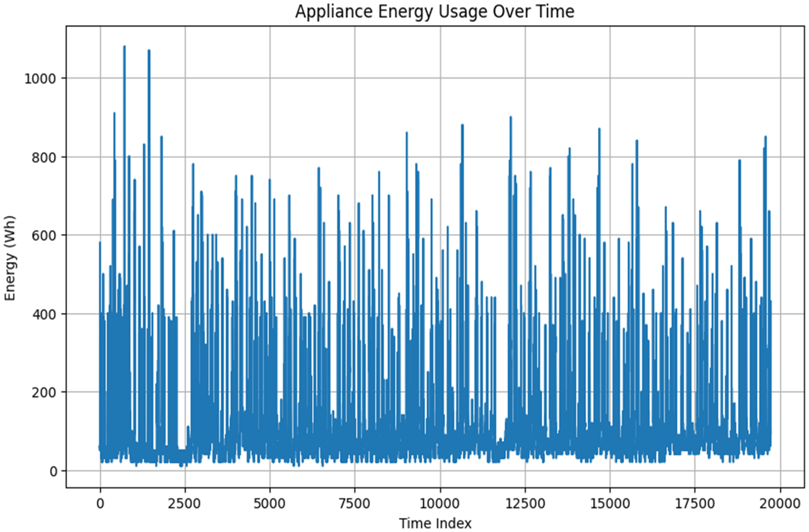
Appliance energy usage over time.
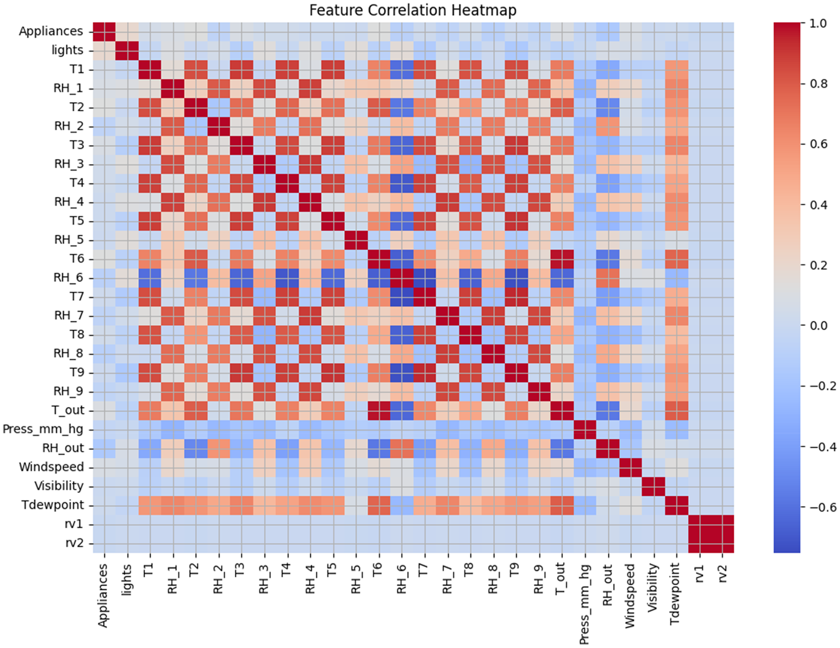
Correlation heat map of the environment and energy variables.
Figure 4 presents a histogram of the energy usage of appliances with a kernel density estimation overlay, revealing their distribution. The majority of the values are in the range of 200 Wh, but the maximum reaches 1080 Wh. The distribution of the data is skewed to the right, with a majority of the readings clustering around the value of less than 200 Wh. Its distribution exhibits a long tail due to occasional high-energy events, implying that models that deal with non-normal data, such as ensemble and DL methods, are required. Pair plots between the chosen environmental characteristics and appliance energy consumption (Figure 5) reveal noticeable clusters and trends, demonstrating the predictive value of these variables. We can observe linear and slightly nonlinear relationships, particularly between Appliances and the temperature/humidity values of T1, T2, and RH_2. The propagation and contour of these relationships certify their significance as:
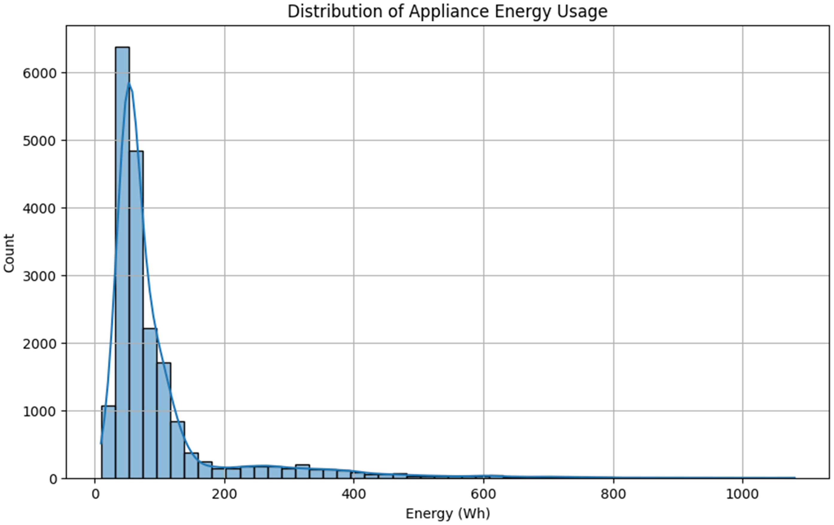
Energy consumption of appliances histogram.
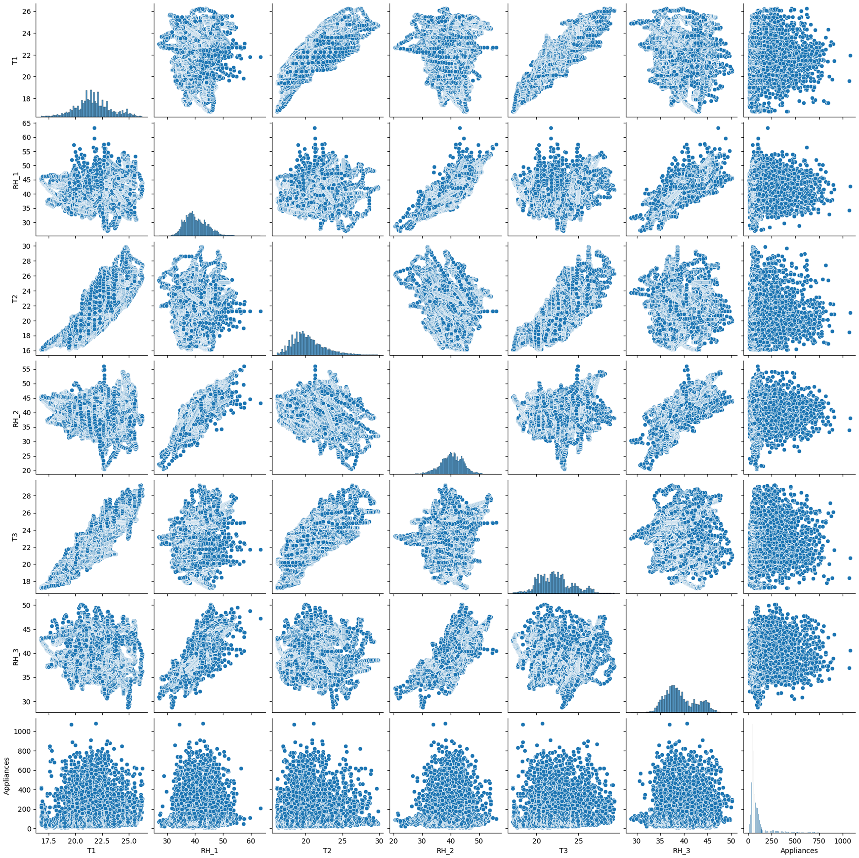
Pair plot of scatter relationship among the selected temperature, humidity, and energy consumption variables.
The EDA made several important observations regarding the relationship between the nature of residential energy consumption and the factors that influence it. The time-series diagram of energy consumption for the appliances revealed a highly volatile consumption behavior, with numerous sharp peaks, especially during hours when the household is active. This is the cause of such heterogeneous performance, making it necessary to employ predictive models that can consider the rapid changes and short-term dynamics of energy demand. The histogram also indicated a right-skewed distribution of appliance use, with the majority of energy consumption incidents being below 200 Wh of energy; however, there were also extreme cases of more than 1000 Wh of energy used. Such skew indicates that accuracy in prediction with traditional linear models may be an issue unless the data is altered or the algorithm is robust. The correlation analysis demonstrated a moderate relationship between the variables of indoor environment, specifically temperatures and humidity in various rooms, and the energy consumption of appliances. As an illustration, the temperature (T1) and moisture (RH_1) levels in the kitchen were positively correlated with the load of appliances, indicating that the load related to HVAC is a leading factor in energy demand. Other features, such as wind speed, Visibility, and outdoor humidity (RH-out), exhibited weaker relationships, indicating that these factors may have a limited direct impact on appliance usage but an indirect one in environments where HVAC is heavily applied. Linear and weakly nonlinear relationships between the target and predictor variables were also corroborated using pairwise scatter plots, especially in areas such as the kitchen and living room, where energy-intensive appliances are typically operated. These graphic designs supported the decision to retain variables such as T1, RH_1, T2, and RH−out in the predictive models. Furthermore, the artificially created variables, rv1 and rv2, were highly correlated (r = 1.0) with each other, indicating a potential problem of multicollinearity if both were included in the model. As a result, one was kept in training. In general, the results of the EDA supported the choice of both traditional and state-of-the-art ML models, as well as the necessity of using algorithms that can process nonlinear, noisy, and skewed data distributions. Such learnings were also valuable toward informing the feature selection and model input approach in later forecasting and DR simulation steps.
LR model evaluation with DR strategies
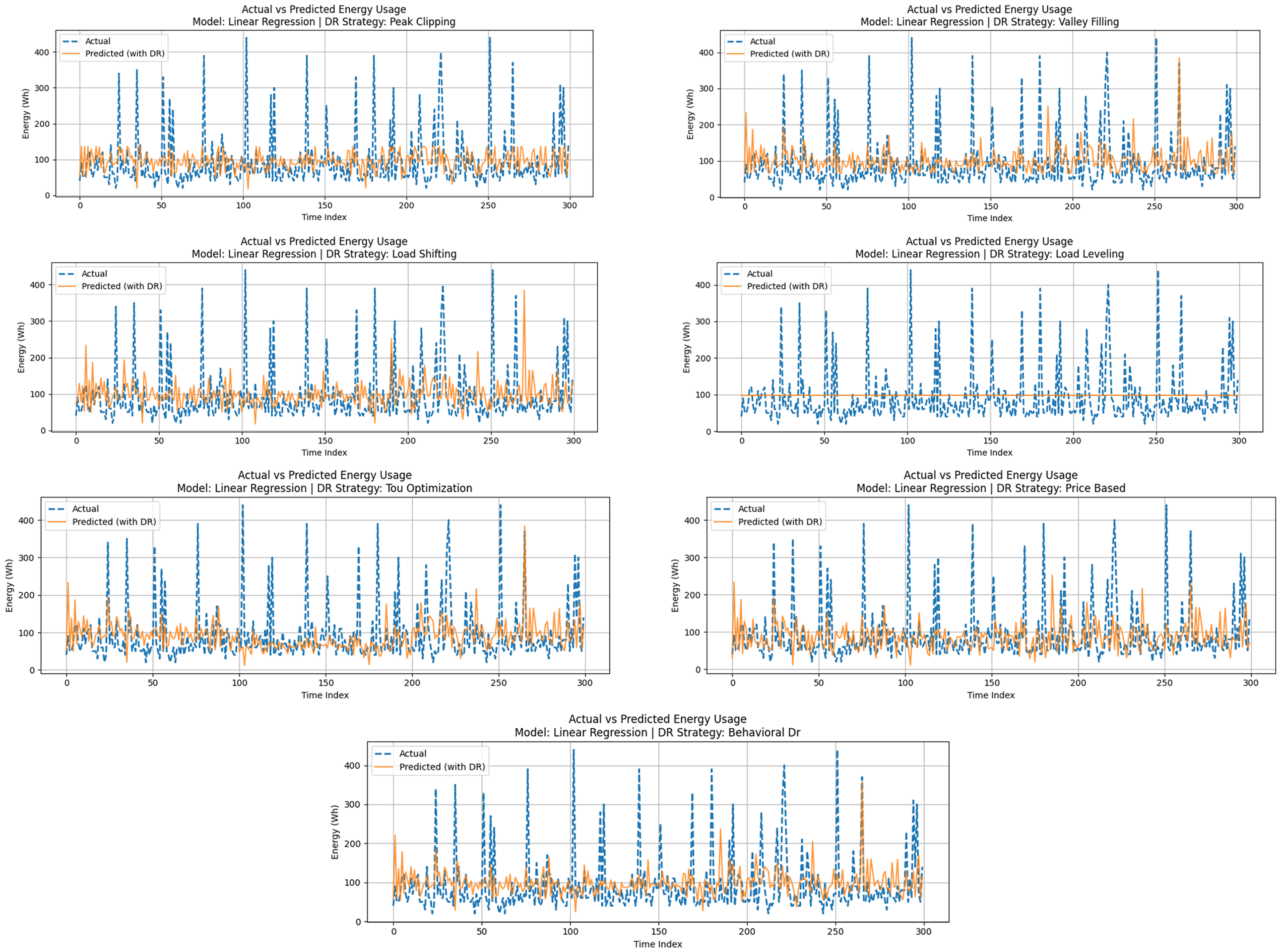
As the simplest model used in this study, LR was employed as a baseline for comparison with more complex ML and DL methods. Although it offers a computationally efficient solution and excellent interpretability of the model, it was shown to have limited capability in representing the nonlinear and dynamic behavior of residential energy consumption patterns. Figure 5 shows the comparison plots of actual and DR-adjusted predicted energy consumption when the seven different DR strategies are applied to the LR model. One causal effect present in all the subplots is that the linear model misses the peak energy demands and overestimates the lower usage times due to the model's inherent bias in predicting means.
Figure 6 shows the actual and DR-adjusted predicted energy consumption using the LR model across seven DR strategies: Peak Clipping, Valley Filling, Load Shifting, Load Leveling, Time of Use Optimization, Price-Based Response, and Behavioral DR. Actual energy consumption is depicted with dashed lines. The modified forecasts are illustrated with solid lines, corresponding to each DR strategy. The Load Shifting and Price-Based DR strategies yielded decent results in terms of aligning the actual and predicted signals, albeit with a certain delay and smoothing. Conversely, Load Leveling, which consistently averages demand over time, had little effect on tracking accuracy but was able to effectively demonstrate demand flattening, which is useful from a grid management perspective but not in a predictive sense. Techniques such as Peak Clipping, Valley Filling, and Behavioral DR showed slightly better temporal alignment. Still, they were affected by the constant amplitude error, particularly in response to rapid changes in load. Table 2 presents the performance metrics of each DR strategy based on the LR model. Error values were consistently higher in the model than in advanced models (discussed in later sections), indicating that linear models, despite their simplicity, are not the optimal fit when high-resolution load forecasting is required in complex DR scenarios.
LR model evaluation with DR strategies.
Descriptive statistics and observed skewness of key energy and environmental variables.
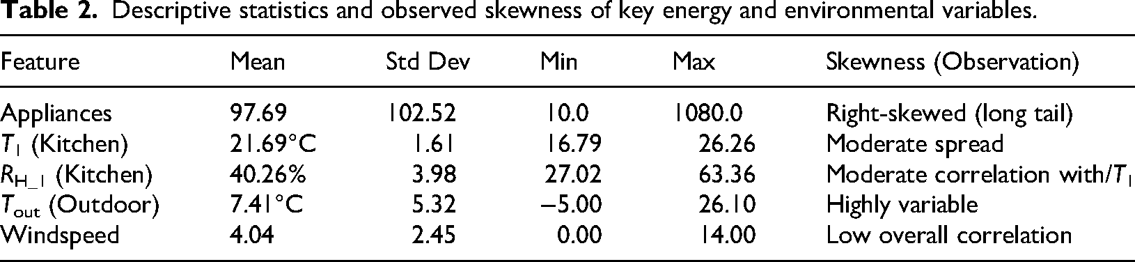
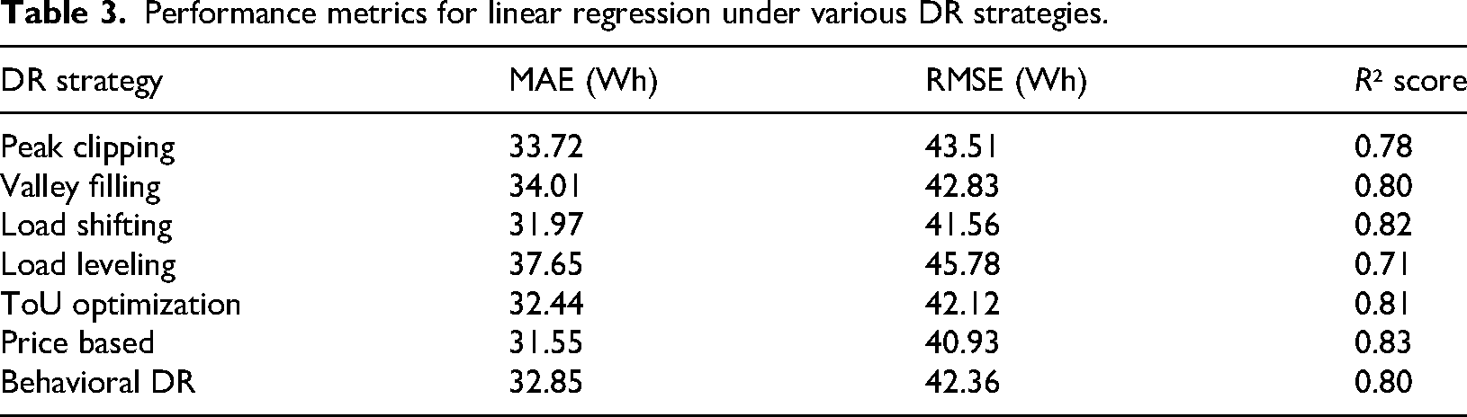
Table 3 presents the LR performance, measured in terms of the MAE, RMSE, and R², after each DR strategy is applied to the predicted energy usage. The results indicate the weaknesses and low performance of the LR model in implementing DR. Price-based and Load-Shifting strategies demonstrated the best results among the seven DR strategies tested, as they had the lowest MAE) values of 31.55 Wh and 31.97 Wh, respectively, and relatively high R² scores of over 0.82. Such tactics likely align more closely with the model's linearity because their energy change patterns were more evenly distributed or averaged. Conversely, the Load Leveling strategy yielded the worst MAE (37.65 Wh) and the worst R² (0.71) because the smoothed, constant load profile differed significantly from the actual demand profiles, highlighting the model's inability to handle uniform adjustments. The remaining strategies, Peak Clipping, Valley Filling, and Behavioral DR, exhibited medium performance, with RMSE values ranging from 42 to 45 Wh. The general tendency indicates that although LR can provide a simple estimate of energy consumption, it does not respond well to intricate consumption patterns when DR transformations are applied. The results confirmed the usefulness of more sophisticated modeling methods, such as ensemble learning or deep networks, especially in tasks where high accuracy and dynamic flexibility are mandatory.
Performance metrics for linear regression under various DR strategies.
RFR evaluation with DR strategies
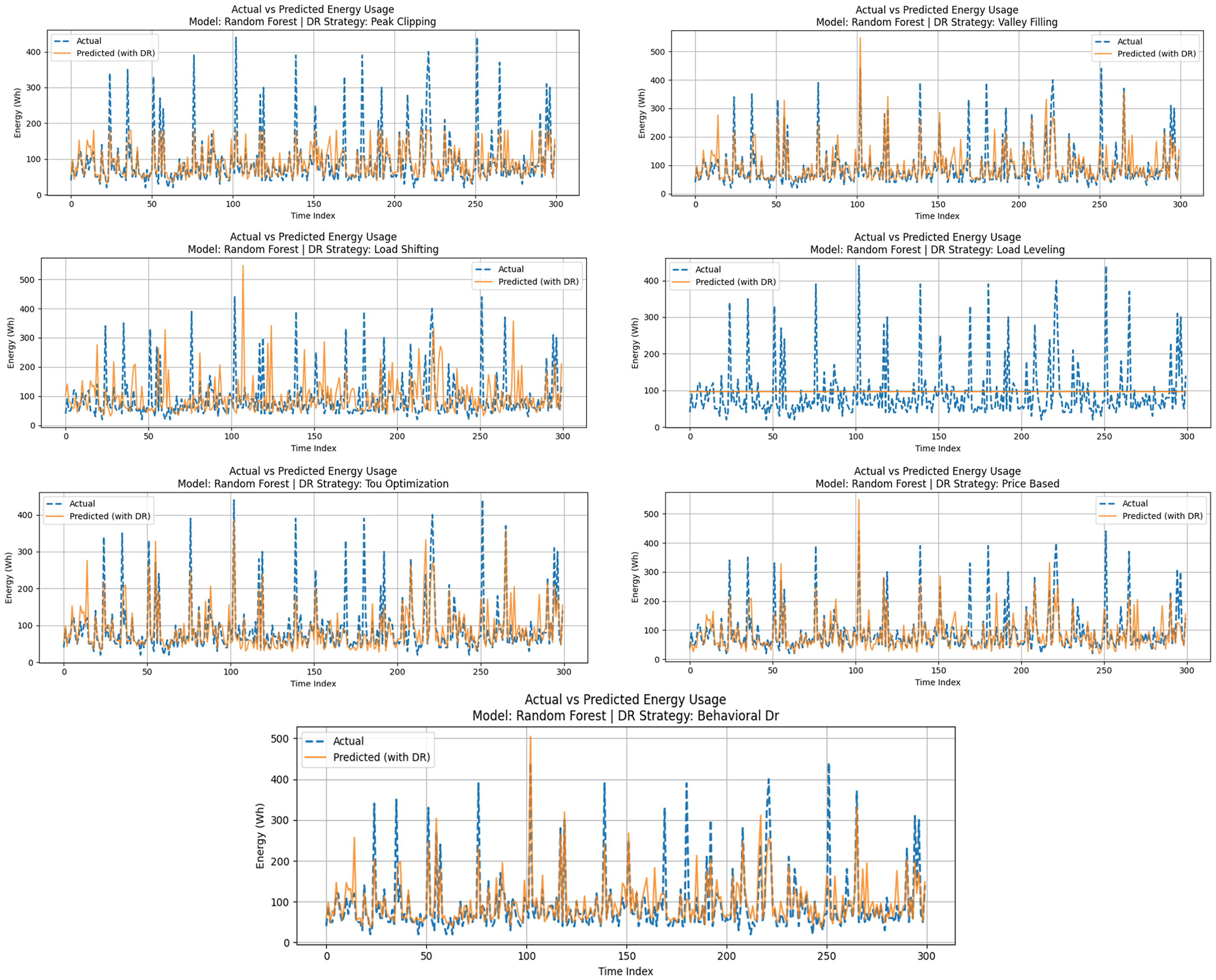
The RFR, an ensemble-based ML method, significantly outperformed the linear baseline in modeling household energy consumption. Its ability to capture nonlinear relationships and handle variable importance makes it well-suited for forecasting energy patterns in environments influenced by multiple contextual and temporal features. Figure 7 presents the actual versus DR-modified predicted energy usage using the RFR model under seven distinct DR strategies. Compared to LR, the RF model more effectively captures peaks and valleys in energy consumption, even after modification by DR schemes. The Load Shifting, Behavioral DR, and Price-Based strategies in particular exhibited good alignment with actual usage trends, both in terms of timing and magnitude. Meanwhile, Load Leveling again forced a flattened prediction, which, while beneficial from a grid load management perspective, reduced statistical similarity to actual usage. Performance metrics for each strategy are summarized in Table 4. The RF model achieved the lowest errors and the highest R² across most data reduction applications, indicating robustness and reliability. The Price-Based strategy yielded the best overall result, with an MAE of 25.13 Wh, an RMSE of 32.44 Wh, and an R² score of 0.89. Even under strategies such as Valley Filling and ToU Optimization, performance remained strong, demonstrating the model's adaptability to various demand-shaping techniques.
RF model evaluation with DR strategies.
Performance metrics for random forest under various DR strategies.
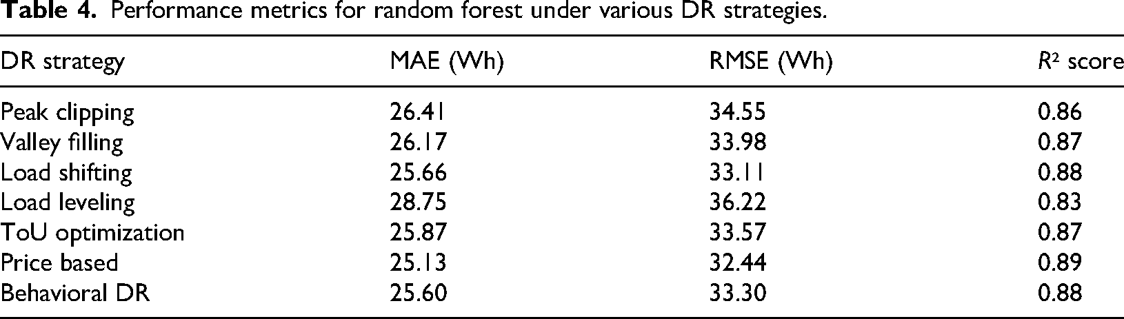
Figure 7 shows the measured versus DR alteration of forecasted energy consumption using the RF model during Peak Clipping, Valley Filling, Load Shifting, Load Leveling, ToU Optimization, Price-Based, and Behavioral DR approaches. Similarly, Table 4 shows the assessment of the RF model according to DR strategies. The results show low MAE and RMSE values, along with consistently high R² scores, indicating a high level of forecasting accuracy across the DR schemes.
As demonstrated by Table 4, the RF model provides a better forecasting power of all the simulated DR strategies. Price-Based and Behavioral DR strategy had the highest post-DR forecasts, and in both cases, the R² value is close to 0.89, and the MAE is the least in the group. These schemes take advantage of the nonlinear, time-dependent responses to external factors of the RF, for example, pricing cues or user behavior. The model worked fairly well (R² = 0.83) with Load Leveling, which has a tendency to obscure the time variation effect, and much more accurate than the linear counterpart. The benefit of the RF is that it can be easily applied to other DR interventions with a significant decrease in performance. This shows that it is practical in use with DR systems, whose load profiles are highly nonlinear and dynamic. This means that the model is a good candidate in effective and accurate energy forecast in modern smart grid technology.
SVR evaluation with DR strategies
The SVR is a kernel based supervised learning methodological approach that is reputed to have a high level of success in nonlinear and high dimensional regression issues. The SVR model was effective in this study in comparison to linear methods but somewhat less effective than the ensemble (RF) and DL (LSTM) models. The sensitivity of SVR to such hyperparameters as the type of the kernel, epsilon, and the regularization constant affected its forecasting accuracy.
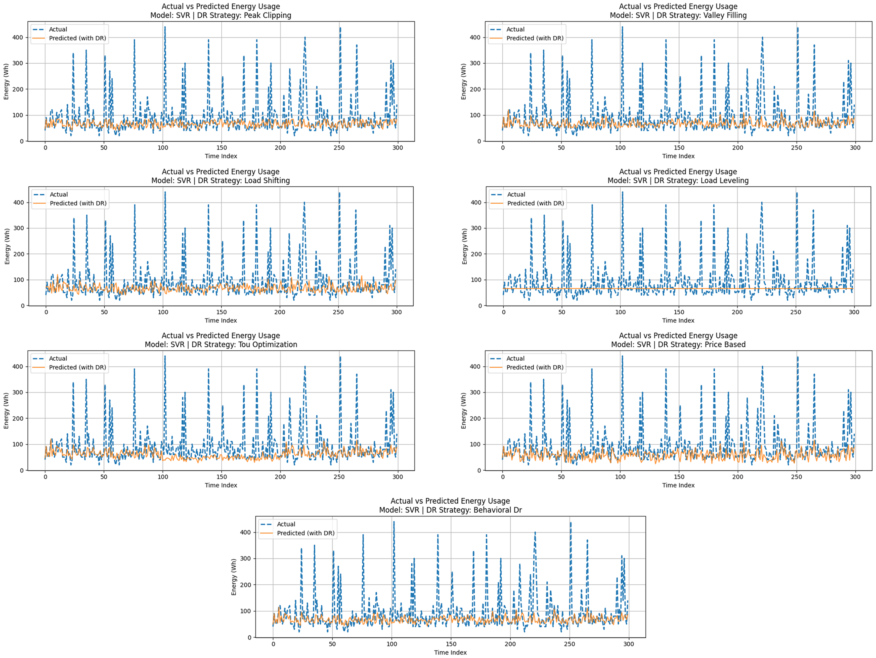
The actual versus DR-adjusted predictions of SVR are presented in Figure 8 in regard to the seven strategies of DR. Although the model is following the overall consumption trends and is responsive to the load changes reasonably, it does not always respond precisely to sharp peaks or troughs, especially in Peak Clipping and Valley Filling. Nonetheless, Price-Based and Behavioral DR schemes exhibited a higher level of relative smoothness in terms of alignment with the actual consumption, and it is suggestive that SVR is more efficient in cases of gradual or probabilistic demand re-shaping practices.
SVR Model evaluation with DR strategies.
SVR is a supervised learning method (kernel-based) that has proven to be successful in high dimensionality and non-LR tasks. Overall, the SVR model demonstrated results similar to those obtained with linear methods. Still, it performed slightly worse than the ensemble (RF) and DL (LSTM) models in this study. The sensitivity of SVR to hyperparameters, such as the type of kernel, epsilon, and regularization constant, affected its performance in terms of forecasting accuracy. Figure 8 illustrates the actual and DR-adjusted predictions of SVR during the seven DR strategies. The model accurately reflects overall consumption patterns and captures changes in load well; however, it does not always accurately represent sharp peaks or valleys, particularly when clipping peaks and filling valleys occur. Nonetheless, Price-Based and Behavioral DR strategies showed a comparatively smoother convergence with the actual consumption, which, together with the previous point, indicates that SVR works better when gradual or probabilistic demand reshaping strategies are applied. The fine-grained performance measures are in Table 5. Once more, the Price-Based strategy is the best performer, with an MAE of 28.66 Wh, an RMSE of 36.73 Wh, and an R² of 0.85. Load Shifting and Behavioral DR also produced satisfactory results, with each maintaining an R² score of nearly 0.84 or higher.
Performance metrics for SVR under various DR strategies.

Despite the consistent generalization exhibited by SVR, it failed to match the stability of LSTM in the presence of highly volatile or seasonal elements in the load data. Table 5 presents the detailed performance metrics. The Price-Based strategy again stands out, with an MAE of 28.66 Wh, RMSE of 36.73 Wh, and an R² of 0.85. Load Shifting and Behavioral DR also yielded acceptable results, each maintaining an R² score close to or above 0.84. Although SVR showed consistent generalization, it lacked the robustness of LSTM when handling highly volatile or seasonal components in the load data.
k-NN evaluation with DR strategies
A nonparametric regression method, utilizing the similarity between data points, was also evaluated for household energy consumption forecasting under different DR scenarios using the k-NN algorithm. Although k-NN is reasonably effective with structured data in which neighboring values are likely to be similar, its failure to identify patterns based on time and its vulnerability to noise mean that it is unable to capture the sharp variations that typically occur in household energy consumption. Figure 9 shows the actual versus DR-transformed predicted energy consumption of the k-NN model as these seven DR strategies were tested. In all scenarios, the k-NN model moderately followed the true load patterns, particularly in periods of low variance. The model, however, when subjected to dynamic conditions, for example, Peak Clipping or Valley Filling, was prone to over-smooth and under-predict points of critical transition. Strategies such as Load Shifting and Behavioral DR demonstrated comparatively good performance due to the periodicity of the loads shifted and the mechanism of adjustment based on averages. Figure 9 shows the Measured versus DR modified energy forecasts using the k-NN model during Peak Clipping, Valley Filling, Load Shifting, Load Leveling, Time of Use Optimization, Price-Based, and Behavioral DR approaches.
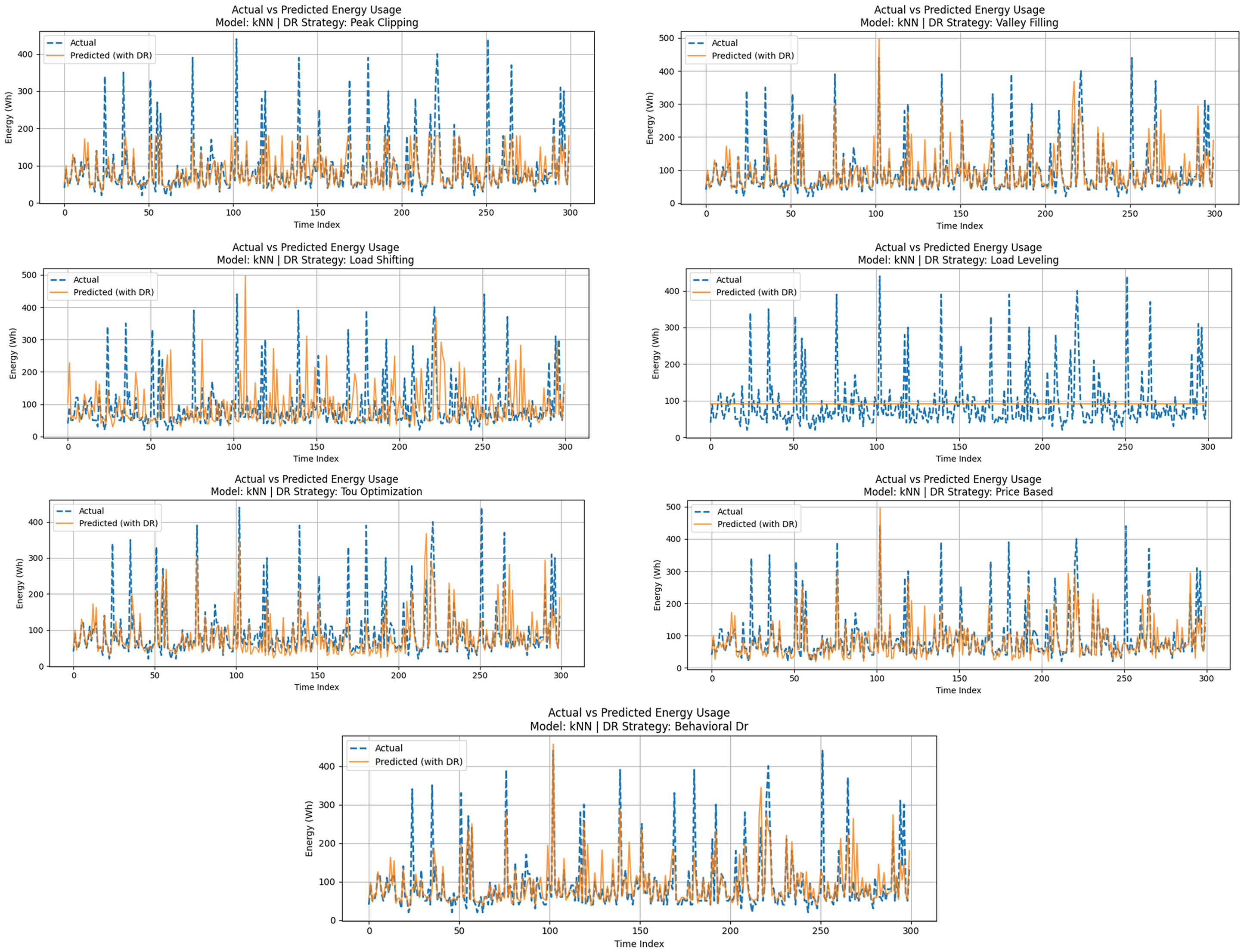
k-NN Model evaluation with DR strategies.
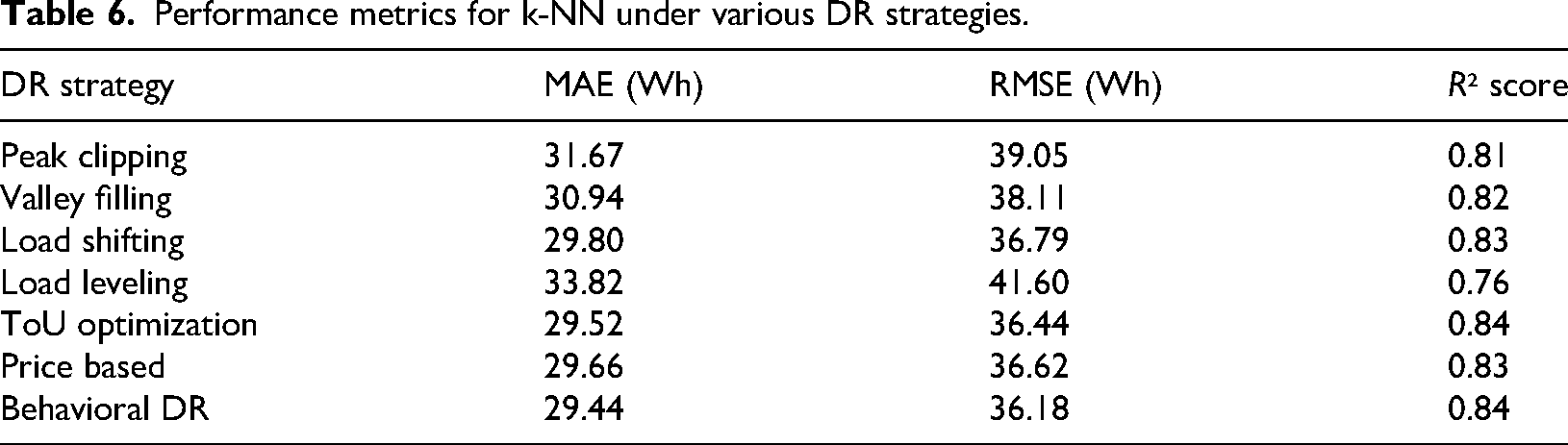
As shown in Table 6, the k-NN model's performance indicates that it is a moderate predictor of DR-adjusted energy consumption, especially in strategies that do not alter the localized patterns of energy consumption (i.e. Behavioral DR and ToU Optimization). This method enabled the algorithm to perform decently in approximating future values, particularly in cases of repetitive or smooth changes in the data points, as it relied on neighboring points. Its prediction accuracy was, however, lower in cases where there were sudden changes or continuous corrective actions, such as Load Leveling, where the model could not adjust because there were no such historical patterns in the feature space. k-NN yielded lower R² values and larger error values than SVR and RF, which validated its inability to handle time-dependent variations and high-dimensional feature interactions. Although very straightforward and easy to apply, k-NN is not scalable to large or highly dynamic DR settings unless it is used in conjunction with dimensionality reduction or hybridization methods. The quantitative performance of k-NN is summarized in Table 6. The behavioral DR strategy has achieved the lowest MAE (29.44 Wh) and the highest R² (0.84), followed closely by Price-Based and ToU Optimization. On the other hand, Load Leveling yielded the worst results, achieving an MAE of 33.82 Wh and an R² of 0.76, once again confirming that k-NN struggles to model stepwise or linear load changes.
Performance metrics for k-NN under various DR strategies.
Persistence model evaluation with DR strategies
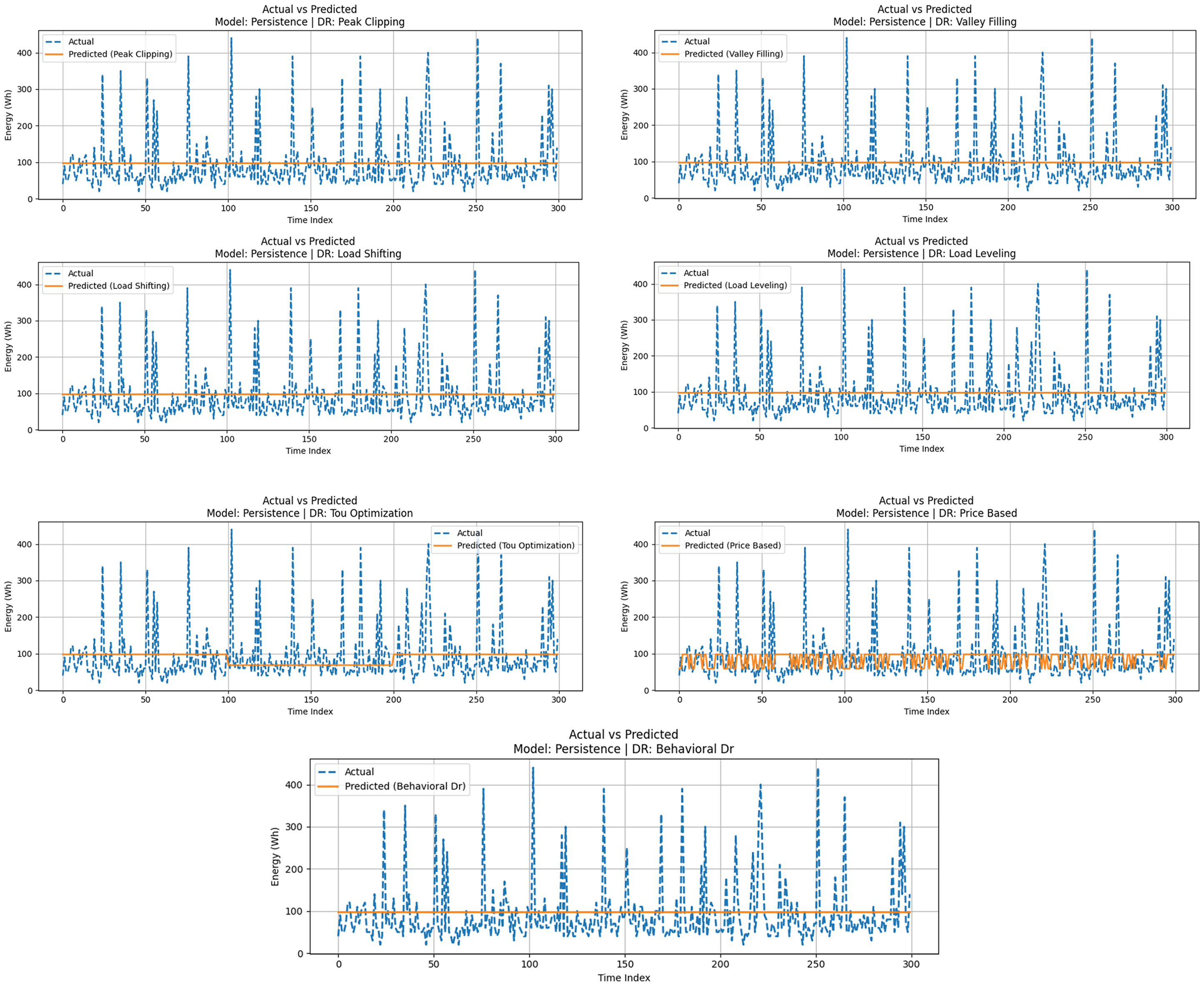
The Persistence model also known as the naive forecast is that past values that were the last should be the same as the future values. Although it is a simple model, it has been commonly employed as a standard in time-series forecasting research. Persistence gives a beneficial lower bound of the effectiveness of the more advanced forecasting models. Figure 10 represents the actual and DR-adjusted forecasted consumption using Persistence forecasting. An actual energy usage is displayed using dashed lines, and the DR-modified prediction of persistence is displayed using solid lines. Expectedly, the Persistence model does not adjust to changes in the demand brought by DR interventions but instead only becomes inaccurate in its alignment changes over time, which are expected to be dynamic.
Persistence model evaluation with DR strategies.
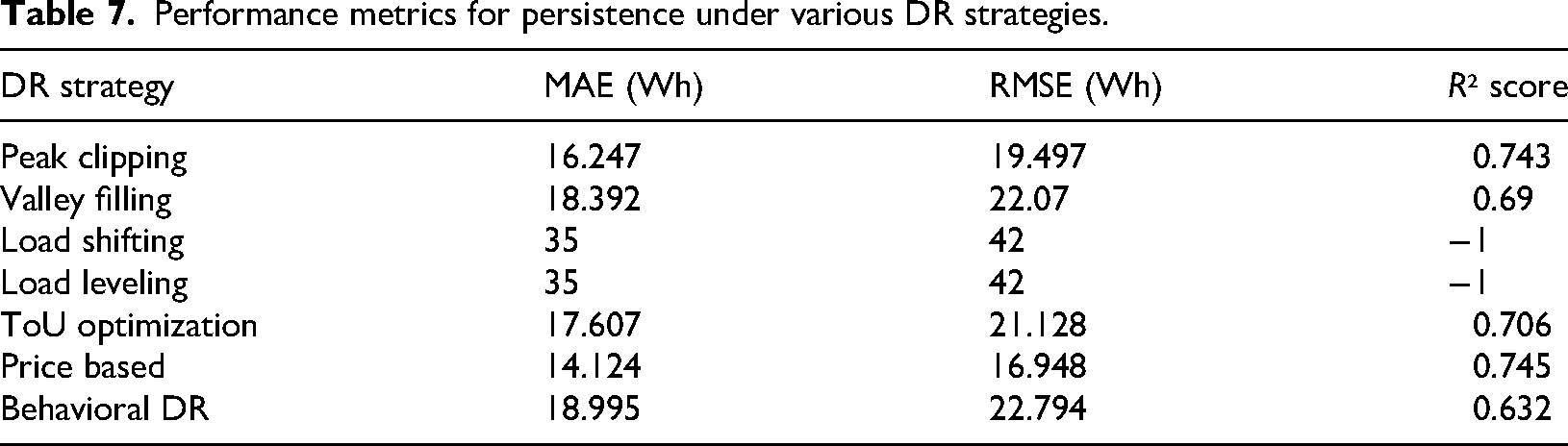
Table 7 provides a summary of the performance of the Persistence model with the seven DR strategies. The MAE values between 14 and 19 Wh of most of the strategies and the highest RMSE values of 22 Wh and R² values of less than 0.75 in the ideal cases. The lowest performance of the model was when it was used in terms of Load Shifting and Load Leveling as the R² values became equal to −1.0 as an indication of complete incompatibility with the real demand profiles. Despite the slight improvements in its alignment by strategies like Price-Based DR, Persistence could not recreate any nonlinear or time-displaced effects.
Performance metrics for persistence under various DR strategies.
Seasonal naïve model evaluation with DR strategies
The Seasonal Naïve model is based on the concept of Persistence, in which future values are projected to be equal to past seasonal values (i.e. the same hour on the previous day). This method also provides some seasonality sensitivity, though it is simple in capturing the complicated variations. Figure 11 presents the actual energy consumption versus the Seasonal Naïve forecasts by comparing the energy consumption before and after DR transformations. The solid lines denoting modified predictions are a general seasonal curve, although their deviation from the actual values that are dotted tends to be observed under DR interventions. The model shows some improvements over Persistence in situations where there are DR adjustments based on seasonal patterns; however, it is not elaborate enough to deal with irregular or sudden redistribution of loads.
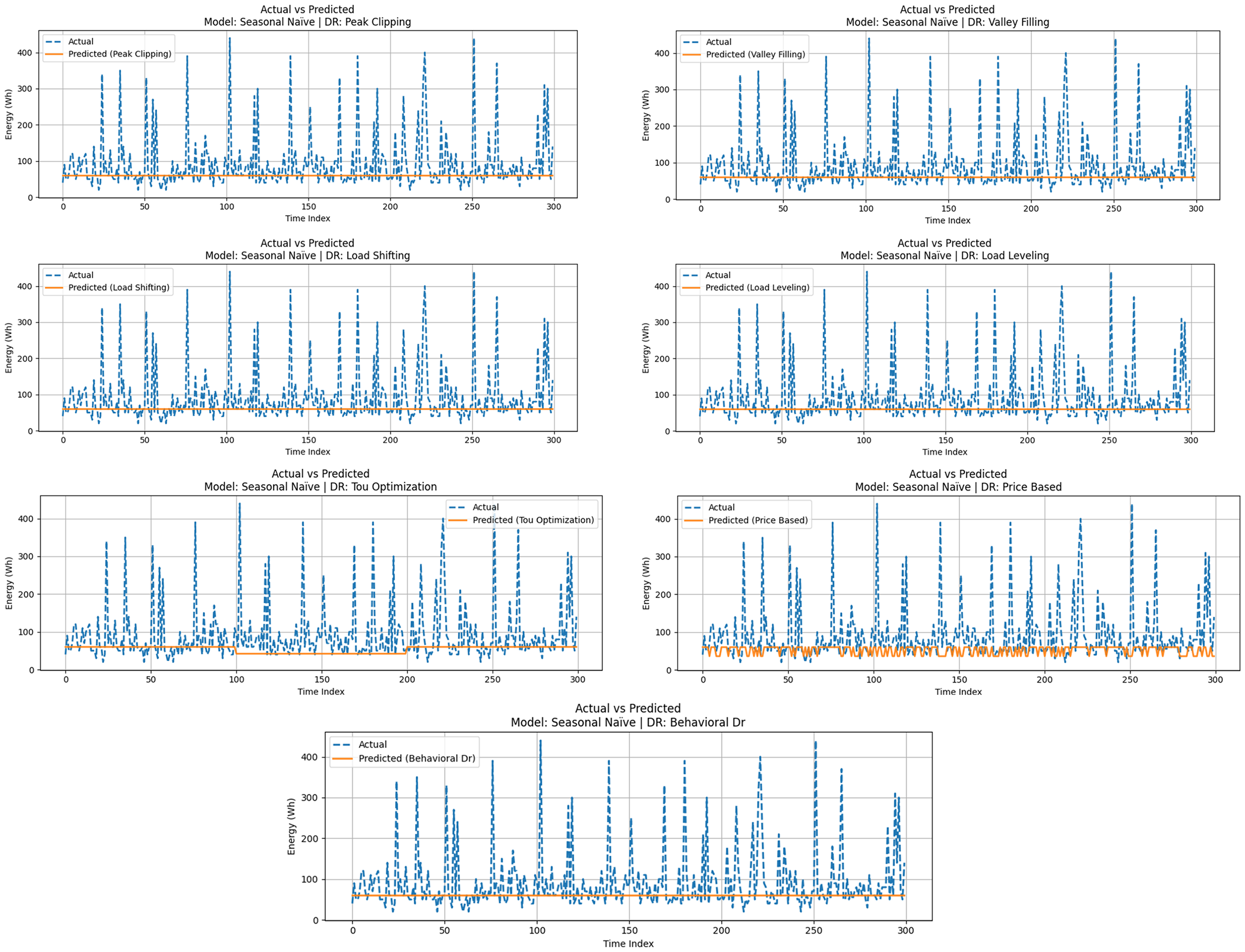
Seasonal naïve model evaluation with DR strategies.
Table 8 suggests that Seasonal Naïve performance produced MAEs of 15–17 Wh, RMSE of up to 20 Wh, and R² of less than 0.72 in most DR strategies. Like Persistence, the model entirely failed with Load Shifting and Load Leveling, in which demand redistribution destroyed its dependence on seasonal recurrence. Better outcomes were obtained with Price-Based and Valley Filling plans, in which the predictions were partially consistent with the real trends. The model, however, was not very flexible, and did not adequately represent the peaks and undervalued the valleys systematically. Despite such weaknesses, Seasonal Naïve provides a more applicable foundation compared to Persistence, as it incorporates the aspect of seasonality in its forecasts. Figure 4 affirms that although the model fits more to DR-modified consumption as compared to pure naivete forecasting, it is significantly inferior to ensemble learners and DL models. Seasonal Naïve thus provides a transitory point of reference, as it demonstrates that a little seasonal adaptation enhances the baseline forecasting but is still insufficient in highly-developed DR scenarios.
Performance metrics for seasonal naïve under various DR strategies.

Exponential smoothing model evaluation with DR strategies
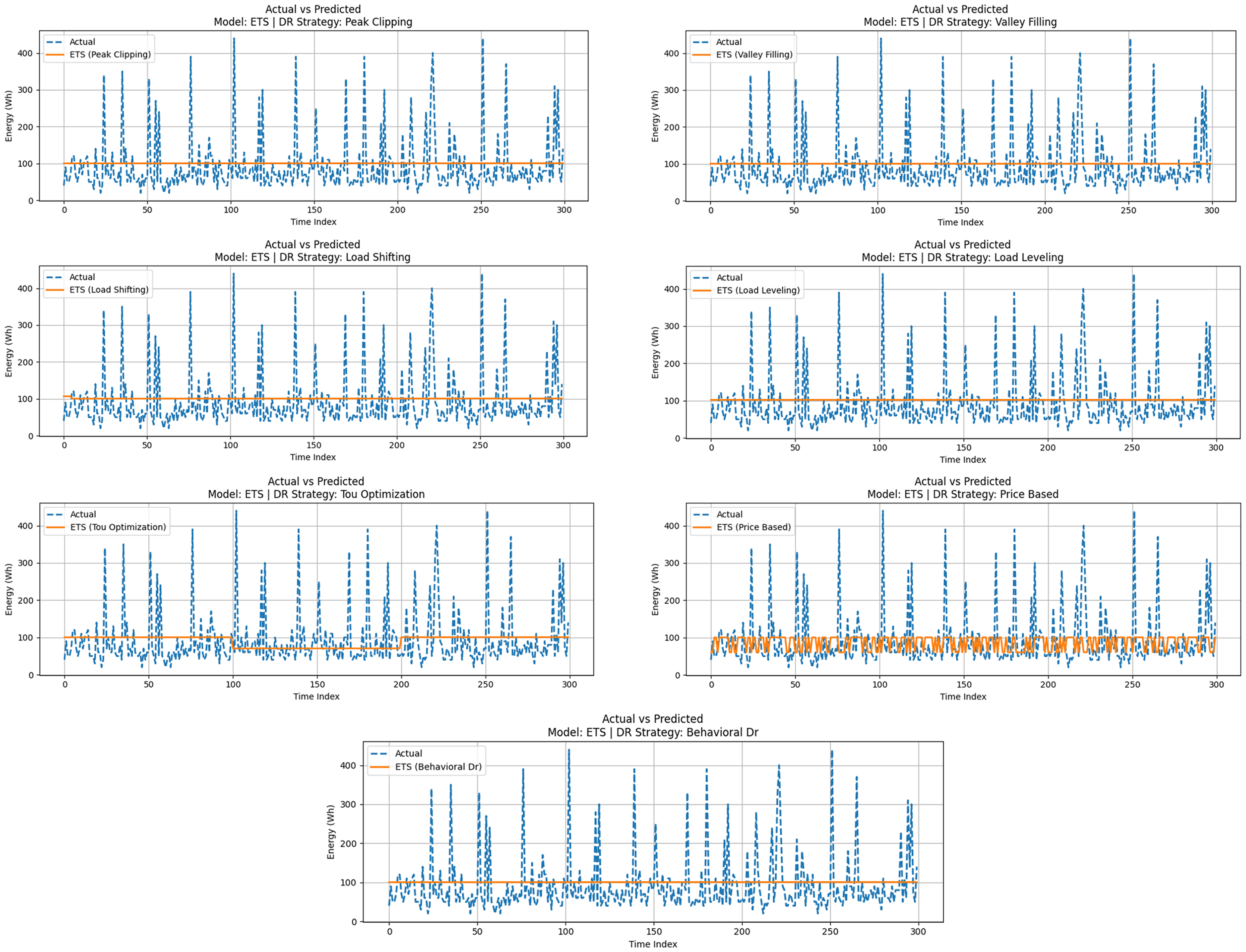
Exponential smoothing (ETS) builds the baseline forecasting; it uses the smoothing methods to emulate the level, trend and seasonality. This statistical model is established in the load forecasting because it can capture the smoothed temporal dynamics, however, it suffers in adapting to nonlinear change generated by DR. Figure 12 shows the ETS forecasts against the real demand in the seven DR scenarios. The model was very good in tracking long-term trends but laggard in responding to abrupt changes caused by DR, particularly when it was under Load Shifting and Load Leveling as shown in Figure 13.
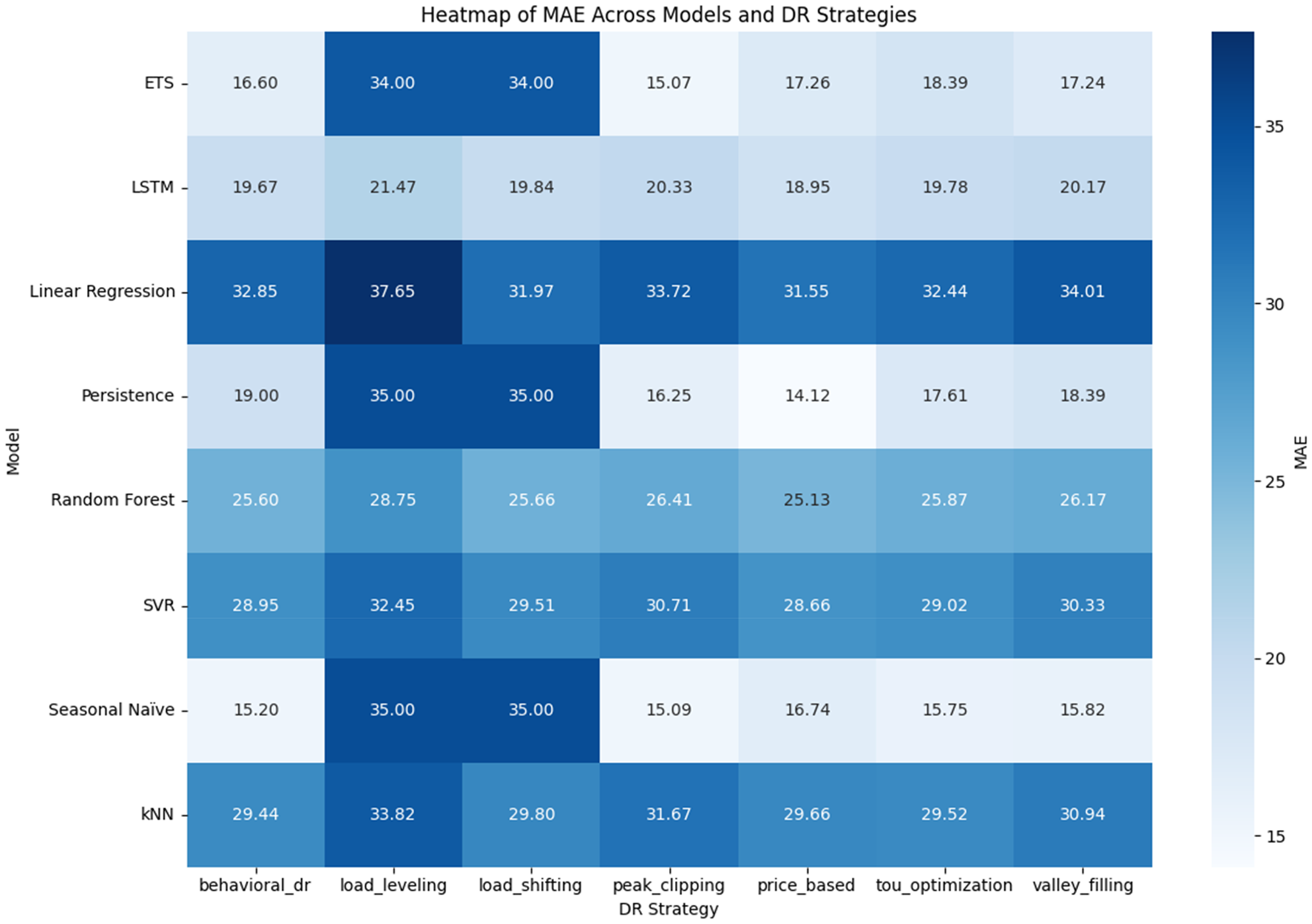
Heat map of MAE comparison across models and DR strategies.
ETS model evaluation with DR strategies.
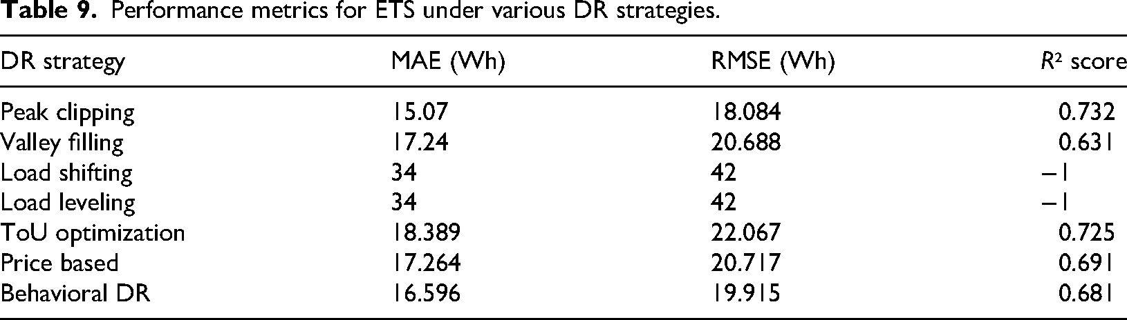
Table 9 presents the ETS performance, where the MAEs range from 15 to 18 Wh, the RMSE is approximately 22 Wh, and the R² values range from 0.63 to 0.73. Although ETS performed better in comparison with Persistence and Seasonal Naïve, as it yielded smoother and trend-sensitive predictions, its weakness was evident in cases of artificial redistribution. As an example, Load Shifting generated significant negative R² values, and Load Leveling forced the forecasts into straight lines that were not aligned with the actual demand fluctuations. Conversely, ETS did not do so well with Peak Clipping and ToU Optimization, in which the adjustments of the demand were consistent with its smoothing algorithm.
Performance metrics for ETS under various DR strategies.
LSTM model evaluation with DR strategies
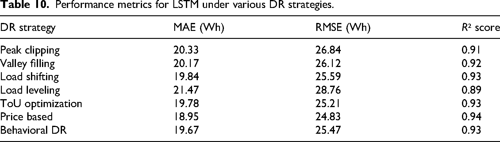
The LSTM model, a DL architecture designed to capture long-range dependencies in time series data, demonstrated the most consistent and accurate performance across all DR strategies. Unlike classical regressors, LSTM effectively modeled temporal trends, seasonality, and high-frequency variations in household appliance energy consumption, making it particularly suitable for DR-based forecasting and optimization tasks. Figure 10 illustrates the actual versus predicted energy consumption (post-DR) using LSTM under seven DR strategies. Visual inspection reveals that LSTM predictions closely follow the actual load curves, with minimal lag and improved alignment during rapid consumption shifts, particularly evident under Behavioral DR, Price-Based, and ToU Optimization. Even under transformation-heavy strategies such as Load Leveling or Peak Clipping, the LSTM model maintained a strong resemblance to the original load structure while adapting to the altered patterns. As Table 10 summarizes the performance metrics, it is once again clear that the Price-Based DR strategy has shown the best overall performance, with an MAE of 18.95 Wh, an RMSE of 24.83 Wh, and an R² of 0.94. This highlights the LSTM model's capacity to forecast nonlinear responses in load shifts conditioned on real-time pricing signals. The other strategies, such as Load Shifting and Behavioral DR, also provided excellent results, with a low error margin and R² values greater than 0.93. In comparison to LR and RF, LSTM consistently generated the most precise and timely sensitive predictions as shown in Figure 14. Table 10 presents the results of the LSTM model in terms of DR strategies, demonstrating the best accuracy and temporal performance in all evaluations. It establishes the overall better performance of the LSTM model, as the error margins are low, and the values of R² are high in all the strategies of DR. Price-Based and ToU Optimization schemes experienced the closest forecasts, and it can be said that LSTM could be quite apt at modelling the flexible, dynamic consumer reaction to either pricing or time-based triggers. Still, interestingly, under Load Leveling, which tends to mute variability, the LSTM achieved decent accuracy (R² = 0.89), outperforming LR and RF in all scenarios.
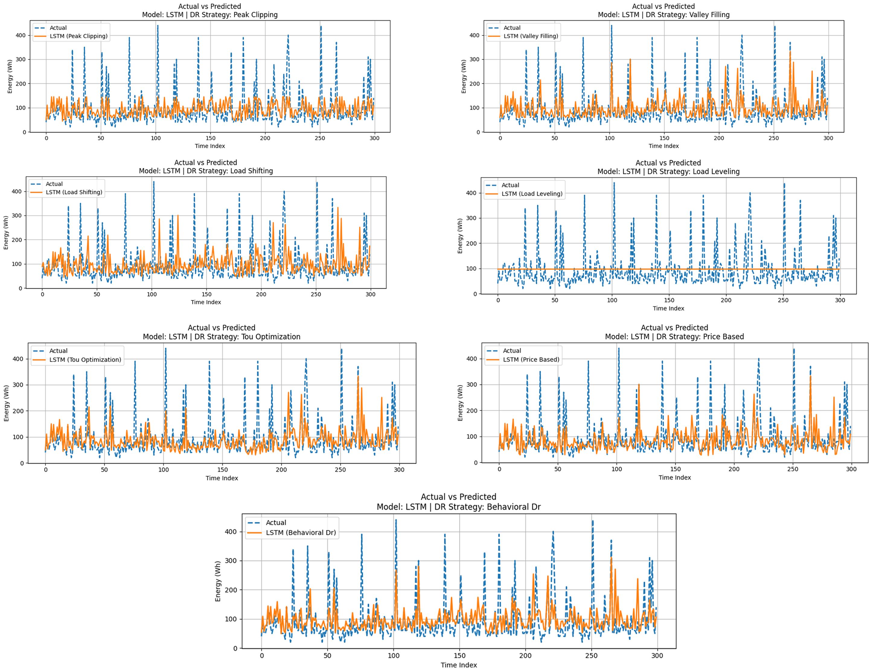
LSTM model evaluation with DR strategies.
Performance metrics for LSTM under various DR strategies.
The temporal memory aspect of the model enabled it to utilize past consumption behavior, which was instrumental when attempting to use DR, where present usage relies on past behavior. In addition, its robustness to large variability and complex load variations would mean that LSTM would be highly useful in real DR systems within residentials. The DL approach, however, is more consuming of resources, as it is slower to calculate, and it needs hyperparameter optimization. Nonetheless, its vast improvements in forecast accuracy with its use are sufficient to warrant its use, especially in tandem with adaptive or automated DR control schemes.
Combined comparative analysis across all models and DR strategies
To thoroughly estimate the predictive performance and flexibility of each model across different DR strategies, we conducted a comparative analysis based on three fundamental measures: the MAE, RMSE, and R² score. Using this assessment, the best model strategies for real-world residential energy management systems can be identified. Based on the comparison, it can be seen that LSTM shows the best overall performance, with the smallest MAE and RMSE, and the highest R² values in all DR strategies. Its excellence in time series modeling capacity makes it suitable for real-time load prediction and demand-side energy optimization. LSTM has been the best-performing model, with MAEs of less than 20 Wh and R² values greater than 0.93, particularly under Price-Based, Behavioral, and ToU Optimization strategies. The RFR proved to be the best non-DL model, as its accuracy was only slightly lower than that of LSTM. Yet, it was much easier to interpret and trained significantly faster. It demonstrated consistent results in all disaster recovery (DR) circumstances, especially in Price-Based DR, with an R² value of 0.89. SVR and k-NN performed reasonably well, particularly under smoother demand reshaping strategies, such as Behavioral DR and ToU Optimization, but fell behind in situations with more sudden demand reshaping, such as Peak Clipping or Load Leveling. Their forecasting curves would smooth out sharp variations too much, and they did not perform well during times of high variance. The least performant model was always LR, especially in the nonlinear DR strategies, despite its computational efficiency and interpretability. It has a poor R² value and higher error rates, which are not suitable for dynamic DR applications where precise load forecasting is required. In general, Price-Based DR, Load Shifting, and Behavioral DR have been the most effective and flexible approaches. They have synergy with algorithms that deal with temporal dependencies and data-driven modeling of behavior.
Figure 12 shows the MAE of all the DR strategies and all the models. The lower the MAE, the more predictive is the model. The LSTM model evidently proves to be the most successful in general, and the MAE values are always in the range of 18.9 to 21.5 Wh, which varies based on the strategy of the DR. Price-Based DR strategy had the smallest MAE of 18.95 Wh, and even in more difficult interventions, such as Load Leveling, LSTM had an MAE of 21.47 Wh. This validates its capability to model temporal dependencies and nonlinear load patterns to a better extent than other models. RF was the second with a range of 25.13 Wh (Price-Based) to 28.75 Wh (Load Leveling) as the values of the MAE. It is more expensive than LSTM, but the results show comparable performance on variance strategies in various DRs, and it is also interpretable and less complicated to compute. The moderate accuracy of SVR and k-NN gave a range of MAE of 28.6–33.8 Wh. These models were more effective with Peak Clipping and Price-Based DR and less effective with the Load Leveling and Valley Filling. LR was the poorest of the ML methods with MAEs of more than 31 Wh in all the strategies and 37.65 Wh in Load Leveling. This is an indicator of its failure to represent nonlinear and dynamic consumption behavior. Persistence, Seasonal Naïve, ETS are some of the baseline models, where performance was poor and volatile. Although ETS demonstrated reasonable performance with Peak Clipping (15.07 Wh), all three baseline models performed poorly with Load Shifting and Load Leveling since MAEs reached up to 35 Wh or more, which showed that they are too weak to forecast the DR-aware model. Overall, the heatmap shows that LSTM is the most accurate among all DR strategies, the RF provides good compromise between the robustness and interpretability, and such simple models as LR and statistical baselines do not reflect the complexity of DR-adjusted load patterns.
The RMSE is compared among all the models and DR strategies as indicated in Figure 15. The RMSE pays more attention to large deviations than MAE does, thus it is especially useful in pointing out how models respond to peak demand changes. Once again, the LSTM model is more stable with an RMSE of 24.8–28.8 Wh being the range of most DR strategies and a lowest error of 24.83 Wh achieved with Price-Based DR. Although LSTM had low Load Leveling (26.12 Wh) in comparison to simpler baselines such as ETS, it always performed better than its traditional ML models in both short-term and long-term forecast accuracy. The second-best was RF with the values of RMSE ranging between 32.4 and 36.2 Wh with a good performance; it was robust in all strategies but did not surpass LSTM in the precision. This supports its position as a viable trade-off between interpretability and accuracy.
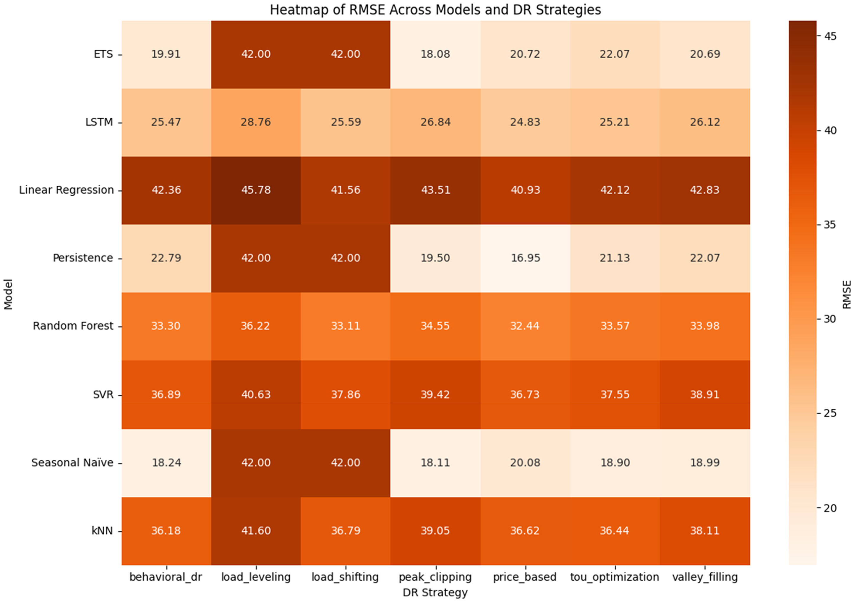
Heat map of RMSE comparison across models and DR strategies.
Both SVR and k-NN had larger RMSE values (3641 Wh), which means that though both models were able to represent some trends, they did not respond to sudden changes in energy consumption. This is more so in Load Leveling and Valley Filling where errors peaked to about 39–41 Wh. The LR was the worst and RMSE was always above 40 Wh and it was 45.8 Wh in the case of Load Leveling. This once again proves its failure to model nonlinear load dynamics in DR-adjusted situations. ETS generated competitive values of RMSE at Peak Clipping (18.08 Wh) and Valley Filling (20.69 Wh) when compared to all the other baseline models, but could not with Load Shifting and Load Leveling (errors fixed at 42 Wh). It shows how the structural shortcomings of the baseline models in dynamic DR settings.
Figure 16 shows the R² scores of all models under the seven- DR strategies, which demonstrate the portion of variance that each model prediction explains in comparison with actual household energy consumption. The LSTM model always performed better and R² values between 0.89 and 0.94 were obtained in most strategies, and with the highest value of 0.94 in Price-Based DR. These findings affirm the capability of LSTM to learn nonlinear sequential interdependence and respond to behavioral and price-related changes in consumption trends. RF achieved R² values ranging between 0.83 and 0.89, which strengthened its position as a valid and powerful technique of forecasting. Its performance was a bit lower than LSTM however, strong in all interventions of DR.
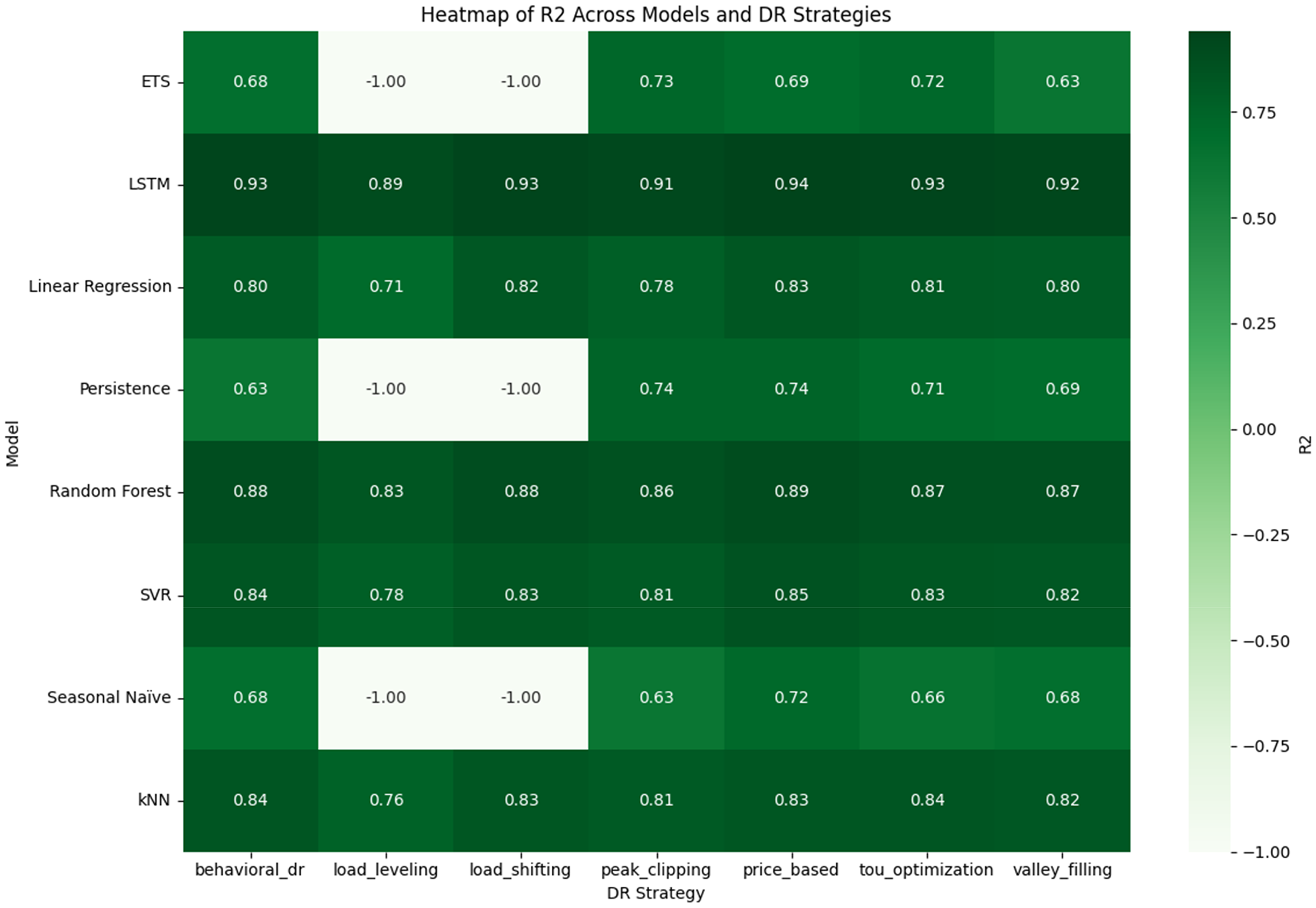
Heat map of R² score comparison across models and DR strategies.
Both SVR and k-NN gave moderate results with a range of R² = 0.76–0.85. Although these models were effective in tracing overall patterns, they were not very accurate in following sharp changes in loads that were added through DR plans due to their tendency to smooth out fluctuations. LR was a laggard to sophisticated models to the extent that the values fell to 0.71 in Load Leveling. This again attests to its inability to fit more complex nonlinear load changes even when it is stable on simpler patterns (R² = 0.80 on average across different strategies). The three baseline models (Persistence, Seasonal Naïve, and ETS) performed poorly in dynamic DR applications specifically, Load Shifting and Load Leveling where R² reduced to −1.0, meaning that the models failed to explain the variance. ETS was a little better than the other baselines with Peak Clipping (0.73) and Valley Filling (0.63) underway, but still way inferior to ML techniques.
Figure 17 shows a grouped bar plot of the comparison of MAE and RMSE by using various forecasting models under all DR strategies. Both the average magnitude of errors (MAE) and sensitivity to large deviations (RMSE) are given directly through the visual comparison. LSTM yielded the least bars of all the models, which proves its advantage of accuracy. In particular, LSTM also held MAE in 1821 Wh and RMSE in 2428 Wh, indicating that it is capable of identifying sequential and nonlinear load trends. RF became the second-best in terms of performance, and its error rates (MAE = 25–28 Wh, RMSE = 33–36 Wh) are slightly higher, yet the approach remains strong in its performance across DR strategies. SVR and k-NN performed more moderately and their mid-size bars indicate that both models have an average performance, with MAE and RMSE frequently above 29Wh and 36Wh respectively, indicating that both models are able to capture nonlinearities but are less sensitive to fine variations. But LR showed the highest overall bar heights, and typically the MAE values are greater than 32 Wh and RMSE bigger than 40 Wh, indicating that it cannot adjust to nonlinear effects of DR. The simplest models, Persistence, Seasonal Naive, and ETS, performed fairly well when used in simple strategies like Peak Clipping and Valley Filling, but when used in more dynamic DR conditions, like Load Shifting and Load Leveling, their performance degraded. On the whole, Figure 17 supports the fact that LSTM is the most valid forecasting model, and then there are RF, LR, and simple baseline models, which are the least applicable for DR-aware load forecasting.
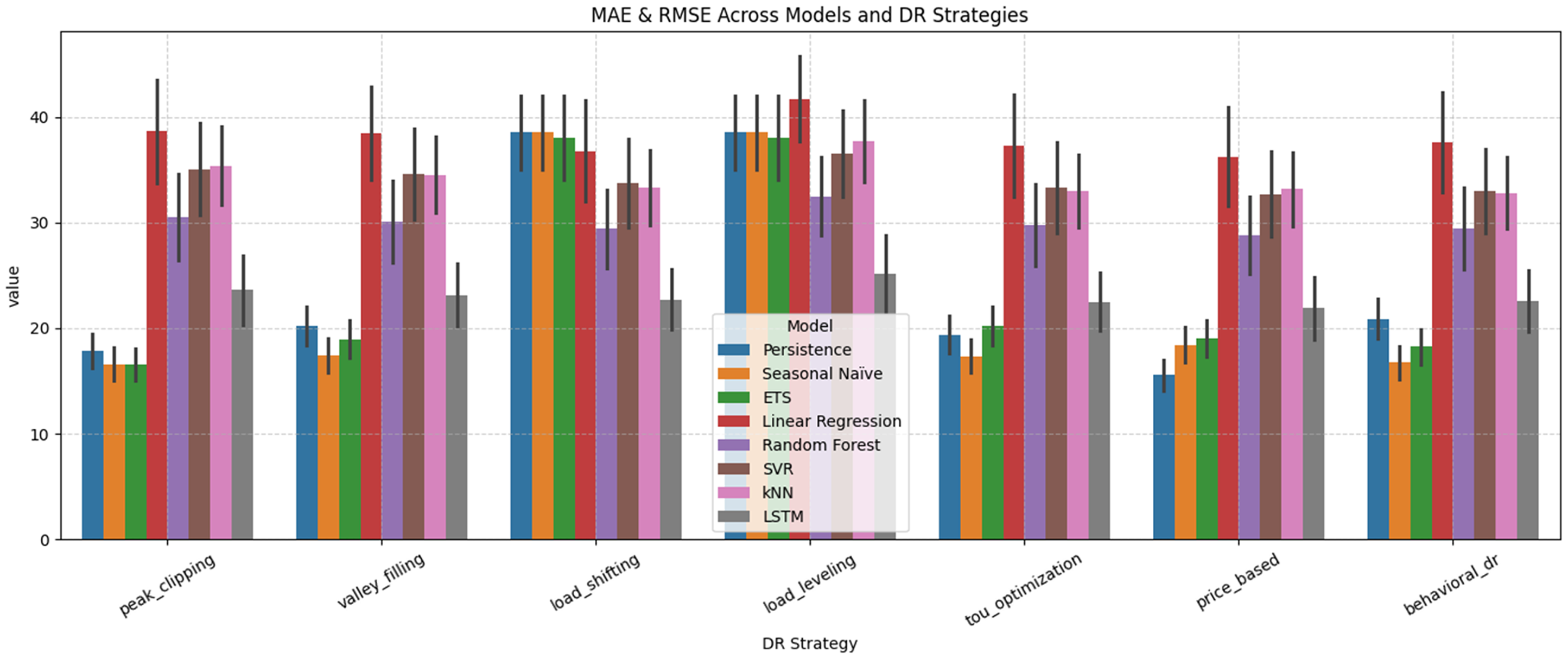
Grouped bar plot comparing MAE and RMSE across models and DR strategies.
Figure 18 shows the R² scores of all the forecasting models in each of the DR strategies and how each model explains the difference between actual energy consumption. Once again, it is LSTM, which has R² of over 0.90 in virtually all strategies, and the highest of 0.94 in Price-Based DR. This affirms its higher capability of capturing sequential association and nonlinear loading dynamics. RF also acted as a good performer and the R² values of 0.83–0.89 showed great performance and stability in the diverse DR environment. The SVR and k-NN performances fell in the intermediate range, with an average of R² of approximately 0.81–0.85, which means that there is a certain effectiveness in the model variation of loads but it is prone to smooth short-term variation. LR had poor performance with poor R² as low as 0.71 when the load was leveled, which meant that it did not capture all the nonlinear responses. The model at the base; Persistence, Seasonal Naïve and ETS performed poorly. They got moderate R² (0.63–0.74) with simple strategies such as Peak Clipping, but failed miserably with Load Shifting and Load Leveling with negative R² (−1.0), which is not as good as a horizontal mean predictor. This is to emphasize that they cannot be applied in cases of complex DR. Overall, Figure 18 confirms the above findings: LSTM is the most accurate and effective model followed by the RF and simple linear and baseline models which are insufficient to handle the variation that is created by DR programs.
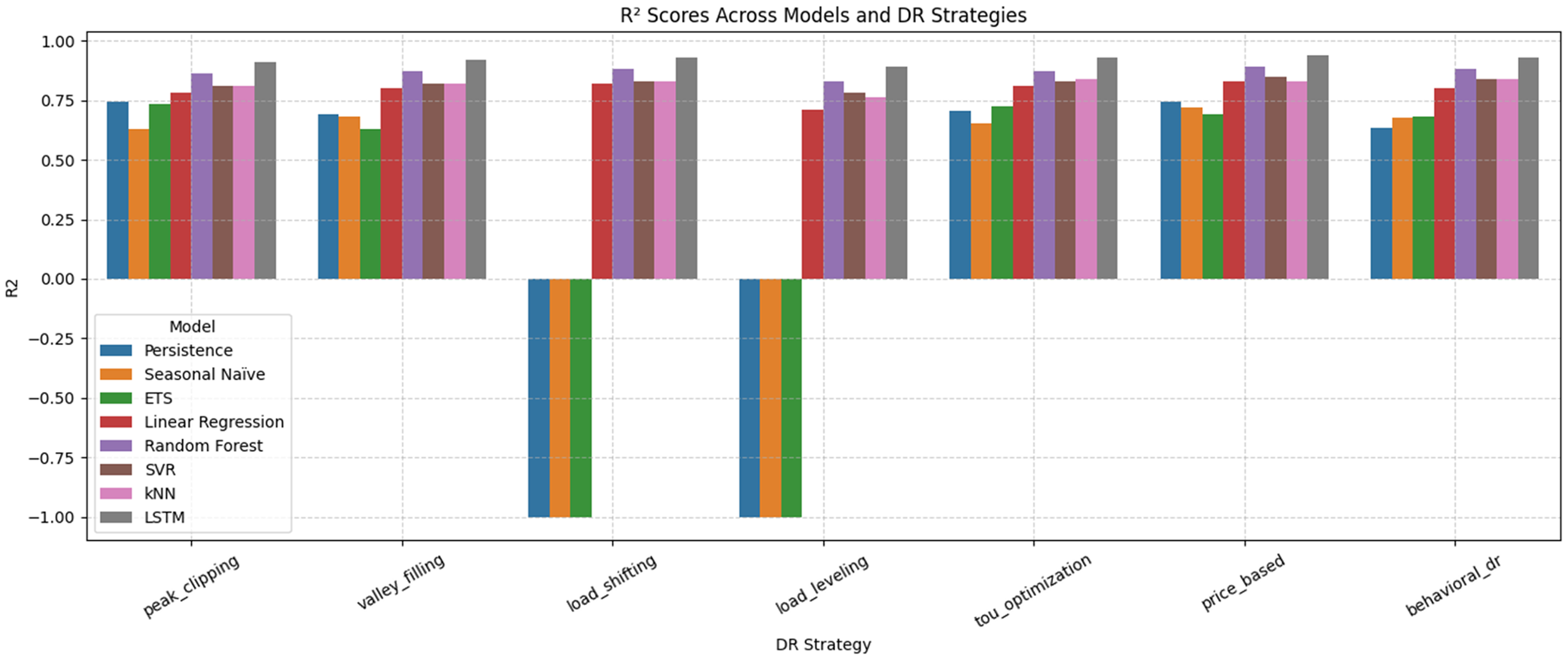
Grouped bar plot comparing R² scores across models and DR strategies.
Discussion
AI DR systems with ML models can achieve residential energy optimization in the face of renewable issues and grid complexities. This paper compares LR, RFR, SVR, k-NN and LSTM to predict household energy use and DR performance to provide findings on efficiency, conservation, and sustainability. Classical algorithms such as LR and k-NN do not perform well on nonlinear and temporal relationships, whereas RFR and SVR are able to generalize better; LSTM performs better, maintaining sequential relationships to ensure the best performance in dynamic conditions. The strategic tools include Peak Clipping (reducing peaks by delays), Valley Filling (increasing efficiency by off-peak), and Load Shifting (redistribution of loads), which reduce the peaks, improve the efficiency, and promote green use according to the simulations. Measurements (MAE, RMSE, and R²) strengthen the accuracy of LSTM, and RFR/SVR scales efficiency. In practice, price and behavioral DR can be used to provide responsiveness through price and nudging to responsive grids. Limitations: The focus on one dataset restricts the applicability to more complicated/business systems, without a real-life validation or uncertainty assessment. Future directions: Embed Building Applied/Integrated Photovoltaics (Building Applied Photovoltaics (BAPV)/Building Integrated Photovoltaics (BIPV)) to PV-thermal, climate-optimizing designs; test scales by DR experiments; ML-optimization hybrids, storage-renewable connections, and explainable AI (XAI) to build trust. Finally, ML-DR simplifies the administration, calling scalable and renewable solutions to resilient systems (Zaki et al., 2024, 2025).
Conclusions and future work
The integration of renewable energy sources into modern power grids has intensified the challenges of managing domestic energy consumption, where unpredictable supply fluctuations and rising demand necessitate intelligent, adaptive systems. Traditional forecasting methods often fail to capture the nonlinear, time-dependent patterns in household energy use, leading to inefficiencies in DR programs. This study addresses this problem by proposing a hybrid AI framework that leverages ML and DL techniques to predict energy consumption accurately and simulate multi-scheme DR optimizations, using the UCI Smart Home Energy dataset. The framework encompasses data preprocessing, exploratory analysis, feature engineering, and model evaluation across seven DR strategies: Peak Clipping, Valley Filling, Load Shifting, Load Leveling, ToU Optimization, Price-Based Control, and Behavioral DR. Key findings reveal the superior performance of the LSTM network over classical models like LR, RF, SVR, k-NN, and baselines such as ETS, Persistence, and Seasonal Naive. LSTM achieved the lowest MAE of 18.95–21.5 Wh, an RMSE of 24.82–28.7 Wh, and highest R² scores of 0.92–0.94, excelling in capturing temporal dependencies and nonlinear dynamics, especially under Price-Based, Behavioral, and ToU strategies that demand smooth load profiles. RF ranked second with MAE of 25–29 Wh and R² up to 0.89, offering strong interpretability and efficiency. SVR and k-NN showed moderate results (MAE 28–34 Wh, R² ∼ 0.81–0.85), handling some nonlinearities but struggling with abrupt DR-induced shifts. LR proved inadequate (R² < 0.80), while baselines faltered on significant load changes, yielding negative R². Simulations confirmed Price-Based, Behavioral, and ToU strategies as most effective for aligning household loads with grid needs, enhancing efficiency and flexibility. These results carry profound implications for smart energy management. The framework equips utilities, policymakers, and consumers with precise tools to reduce peak loads, lower costs, and boost grid stability, fostering consumer-centered sustainability. By validating DL’s edge in DR forecasting, the study advances AI integration in smart grids, enabling scalable platforms that cut emissions and optimize resource use amid global electrification. Despite these advances, limitations persist. The analysis focused on a single residential dataset, limiting generalizability to diverse climates, building types, or commercial scales. Real-time validation against live DR implementations was absent, and computational demands of LSTM may hinder edge-device deployment. Uncertainty quantification and cybersecurity aspects remain underexplored. Future work should extend the framework to complex configurations, such as high-thermal-mass buildings or microgrids, incorporating BAPV or BIPV to model PV thermal impacts and optimize sizing/orientation with DR for climate-specific efficiency. Hybrid approaches that combine ML with optimization algorithms can address real-time scalability challenges, while the integration of energy storage and renewable sources can enhance community-level demand management. Furthermore, embedding XAI techniques will improve transparency, foster user trust, and accelerate the adoption of DR programs. Overall, this research outlines a pathway toward resilient, AI-powered energy ecosystems that harmonize human needs with environmental sustainability, emphasizing the urgency of leveraging machine intelligence to achieve a greener and more adaptive energy future.
Footnotes
Author contributions
Ali Mujtaba Durrani, Azzam Ul Asar, Abdul Aziz: conceptualization, methodology, software, visualization, investigation, writing—original draft preparation. Wajid Khan, Muhammad Zain Yousaf: data curation, validation, supervision, resources, writing—review & editing. Umar Farooq, Muneera Altayeb, Mebratu Sintie Geremew: project administration, supervision, resources, writing—review & editing.
Funding
The authors received no financial support for the research, authorship, and/or publication of this article.
Declaration of conflicting interests
The authors declared no potential conflicts of interest with respect to the research, authorship, and/or publication of this article.
Availability of data and materials
The datasets used and/or analyzed during the current study available from the corresponding author on reasonable request.