Sage Journals: Discover world-class research

Abstract

Supercritical/dense-phase CO₂ pipeline transportation is a critical link in carbon capture, utilization, and storage technology, which is a major approach to reducing emissions. The thermo-hydraulic simulation of CO₂ pipelines usually applies numerical methods developed for oil and gas pipelines. However, the CO₂ properties are highly sensitive to temperature and pressure, compared to natural gas, which may lead to numerical instability. This study improves finite volume method (FVM) with staggered grids and an explicit discretization method of convective terms. The results show that under conditions with rapid flow state changes, the improved FVM enhances the computational stability. Additionally, an adaptive time-step adjustment algorithm is introduced to dynamically adjust the time step based on the rate of flow state changes, ensuring both computational accuracy and efficiency. The proposed algorithm is validated with a pipeline shutdown scenario, where the fluid state along the pipeline undergoes relatively intense changes, demonstrating the stability of the numerical solutions proposed. Furthermore, a comparative analysis of water hammer pressure during shutdown is conducted with theoretical equations and simulations, showing that in addition to direct compression pressure, the pipeline endpoint is also subjected to fluid packing pressure, which should be considered in water hammer control.

Keywords

numerical solution finite volume method self-adaptive time step simulation

Introduction

The development of carbon capture, utilization, and storage (CCUS) is crucial for mitigating greenhouse gas emissions, thereby protecting the environment (Ojuekaiye, 2024). Supercritical/dense-phase CO₂ pipelines are a primary approach to transport large amounts of CO₂ over long distances, considering the investment over the life cycle (Dong et al., 2025). The numerical simulation and flow assurance for supercritical CO₂ pipeline transportation are critical to the successful implementation of CCUS projects (El-Kady et al., 2024; Kim et al., 2024; Li et al., 2025). Commercial software, such as OLGA and Ledaflow, which are primarily developed for multi-phase flow and natural gas pipeline simulation, have been adapted and adjusted for CO₂ fluid pipeline in recent years (Aursand et al., 2013; Drescher et al., 2017). OLGA and Ledaflow have become primary tools in CO₂ pipeline design and flow assurance analysis.

The simulation accuracy and numerical convergence of CO₂ pipeline flow models are influenced by several key factors, including the choice of equations of state (EoSs), formulation of conservation equations, discretization methods, and numerical solving approaches. Reliable EoSs play a crucial role in the simulation of engineering design and hazard scenario identification (Raimondi, 2014). Existing oil and gas fluid equations, such as Peng–Robinson (PR) (Peng and Robinson, 1976), Soave-Redlich-Kwong (SRK), and GERG-2008 (Kunz and Wagner, 2012), can be used to calculate CO₂ fluid properties, along with the SW equation (Span and Wagner, 1996) specifically for pure CO₂. Each of these equations has its own advantages and disadvantages in terms of accuracy, computational speed, and applicable range. Based on comprehensive analysis, the PR and GERG-2008 are suggested in CO₂ fluid properties modeling by DNVGL-RP-F104 (2021) and ISO 27913:2016 (2016) standards, respectively, and are widely adopted in both research and industrial applications. Comparative studies (Botros et al., 2017; Diamantonis et al., 2013; Luo and Chirkov, 2021) have evaluated these models, demonstrating that GERG-2008 offers superior predictive accuracy on vapor–liquid equilibrium, density, entropy (Luo and Chirkov, 2021), and decompression wave speed (Botros et al., 2017). However, the applicability of GERG-2008 model has a limited component library, resulting in reduced predictive accuracy when impurities such as CO, Ar, or H₂ are contained in fluid. Furthermore, the mathematical complexity of GERG-2008 demands greater computational effort, making it more resource-intensive compared to the PR equation.

The homogeneous equilibrium mixture (HEM) model, two-fluid model, and drift-flux model are usually applied in pipeline simulation. Because CO₂ fluid is typically controlled in the dense or supercritical phase during normal pipeline operation, HEM model is suitable for most operating conditions. It is widely employed to simulate the flow characteristics of CO₂ pipelines, such as normal operation (Lu et al., 2024), rupture scenario (Martynov et al., 2018; Munkejord et al., 2021; Zheng et al., 2017), and line packing process (Martynov et al., 2024). The continuity, momentum, and energy conservation equations are applied in HEM model as governing equations to describe flow behavior, offering high computational efficiency and robust numerical stability.

The application of two-fluid model and drift-flux model in CO₂ pipeline simulation is compared (Aursand et al., 2013). Two-fluid model is widely applied in pipeline simulations due to its physical comprehensiveness, but it is mathematically challenging to solve. In contrast, drift-flux model is mathematically well-posed, but its accuracy is limited to specific flow regimes. In the event of a pipeline rupture or gas release, a decompression process may lead to rapid phase transition and flow regime changes; two-fluid model is more recommended to be adopted to achieve more accurate predictions of decompression wave speed and pressure (Brown et al., 2014).

Employing stable and efficient numerical methods to solve the governing equations is crucial for simulations. Both finite difference method (FDM) and finite volume method (FVM) can be used for discretizing partial equations. FVM, in most cases offering better conservation properties and numerical stability (Liu et al., 2013), is typically employed by mainstream commercial software. An explicit FVM is applied to handle the homogeneous flow equations, simulating the phase transition process of supercritical CO₂ fluid within pipelines (Martynov et al., 2016). FDM employs differences to approximate differentials. Although the underlying principle of these two discretization methods differs, the discrete equations derived can be identical under certain conditions, such as in the case of the central scheme in FVM and central differencing in FDM. An implicit central difference method has been utilized for transient simulations of supercritical CO₂ pipelines, where the fluid operates above the critical pressure (Lu et al., 2024). An explicit difference method can be used for the simulation of relatively quick state variations of the pipeline, such as leak or venting scenarios. While the Courant-Friedrichs-Lewy (CFL) condition must be considered to ensure stability and accuracy in both steady-state and transient simulations, it requires a relatively small time step (Teng et al., 2016). Especially, the method of characteristics (MOC) transforms the partial differential equations into a set of ordinary differential equations along the fluid wave propagation paths (i.e. the “characteristic lines”) to achieve high computational efficiency, which is especially designed for a fast transient process of one-dimensional pipeline simulation. Yu et al. (2024) utilize MOC to simulate the rupture process of a pure CO₂ pipeline, based on which the risk of crack propagation under different phase states is analyzed. In addition to simulations inside the pipeline, it is also necessary to conduct dispersion characteristics of CO₂ leakage, since it poses a risk of personnel suffocation (Bielka et al., 2024).

Current thermo-hydraulic simulation methods for CO₂ follow the simulation algorithms used for oil and gas fluid pipelines (Xu et al., 2025). Compared to natural gas pipelines, the physical properties of CO₂ fluid exhibit more drastic variations with temperature and pressure, leading to oscillations in numerical solutions. This paper conducts a stability improvement of FVM algorithms specifically for CO₂ pipelines. An FVM algorithm, combined with a staggered grid scheme and an adaptive time-stepping strategy, is developed to enhance the numerical stability of CO₂ pipeline simulations.

In this paper, the second section details the governing equations for transient simulation, the discretization methods employed, and the boundary conditions. The third section presents a case study of pipeline shutdown operation. It compares the numerical solutions obtained from FVM and improved FVM. Based on the simulation result and water hammer mechanism, the applicability of liquid water hammer formulas to supercritical/dense-phase CO₂ pipelines is analyzed, and water hammer control measures during pipeline shutdown are proposed.

Thermo-hydraulic simulation model

A thermo-hydraulic coupled transient simulation model for a CO₂ pipeline is established based on an HEM model. Because GERG-2008 offers relatively high computational accuracy, while all fluid components involved in this study are covered by the database, the model is built referring to ISO 20765-2:1015 (2015), to calculate the fluid properties involved in the equations, including fluid density, enthalpy, viscosity, and Joule–Thomson (JT) coefficient. Among these, density and enthalpy are directly used for solving thermo-hydraulic equations, viscosity for calculating the hydraulic friction factor, and the JT coefficient for calculating the temperature drop across valves.

Governing equations

The state parameters of a pipeline with space and time are described by the continuity equation, momentum equation, and energy equation. The differential forms are given by equations (1) to (3). Due to the high density of supercritical/dense-phase CO₂, the pressure along the pipeline is sensitive to elevation changes. Thus, it is necessary to consider elevation variations in the model.

A \frac{\partial ρ}{\partial t} + \frac{\partial m}{\partial x} = 0

(1)

\frac{\partial m}{\partial t} + \frac{1}{A} \frac{\partial}{\partial x} (\frac{m^{2}}{ρ}) + A \frac{\partial P}{\partial x} + \frac{λ m | m |}{2 d A ρ} + \frac{A ρ g d s}{d x} = 0

(2)

\frac{\partial}{\partial t} (h ρ - P + \frac{m^{2}}{2 A^{2} ρ}) + \frac{\partial}{\partial x} (\frac{m}{A} h + \frac{m^{3}}{2 A^{3} ρ^{2}}) + \frac{4 K (T - T_{U})}{d} + \frac{m g}{A} \frac{d s}{d x} = 0

(3)

where A is the cross-sectional area of the pipeline, m²; ρ is the fluid density, kg·m⁻³; m is the gas mass flow rate, kg·s⁻¹; x is the axial dimension, m; P is the gas pressure, Pa; λ is the friction coefficient; d is the inner diameter of the pipeline, m; h is the enthalpy, J·kg⁻¹; K is the overall heat transfer coefficient, W·m⁻²·K⁻¹; T and T_U are the fluid temperature and ambient temperature, respectively, K; and s is the elevation, m.

The flow regime of supercritical/dense-phase CO₂ pipelines is generally in the turbulent region. However, the actual gas velocity is relatively low compared to natural gas pipelines, and the flow pattern varies over a wide range, covering the hydraulically smooth region, mixed friction region, and hydraulically rough region.

The convective term, that is, the second term in momentum equation (2) can be neglected in the following analysis, due to the low gas velocity when compared to the sound speed in the fluid, which corresponds to a flow with a low Mach number.

The absolute value of the mass velocity is handled with equation (4). This method enables faster computation, compared to introducing an absolute value function, where ε is an extremely small value to ensure the radicand is non-zero in mathematical operations:

| m | = (m^{2} + ε)^{0.5}

(4)

Discretization method

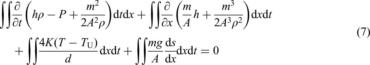
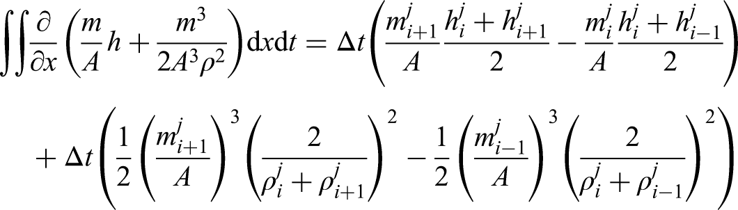
The partial equations (1) to (3) are discretized using FVM with collocated and staggered grids, respectively. The difference of grid partitioning methods for the approaches illustrated in Figure 1, where the horizontal coordinate represents the axial direction of the pipeline, and the vertical axis denotes the time dimension. The space and time step for the two different schemes are Δx and Δt, respectively; and the pipeline length is denoted as L.

Figure 1.

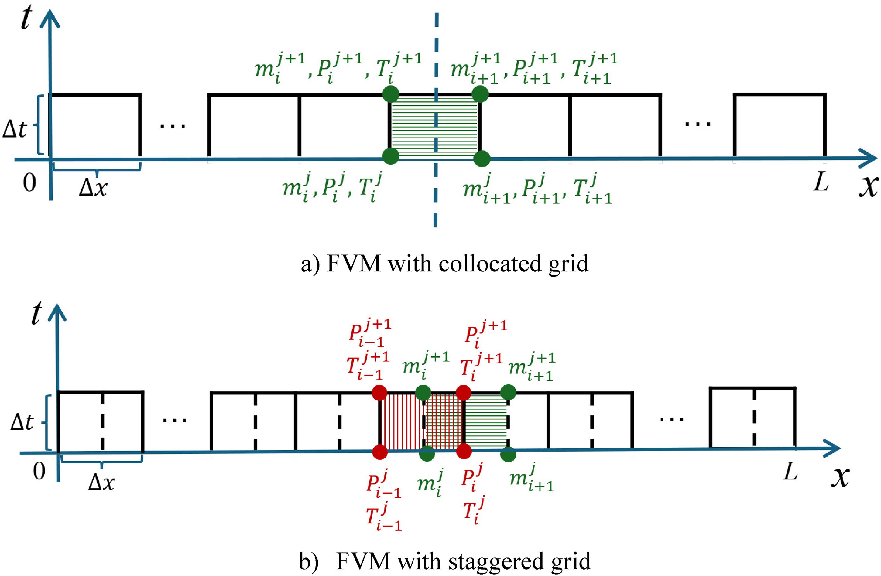
Schematic diagram of FVM with (a) collocated and (b) staggered grids. All flow variables are defined at the cell nodes in the collocated arrangement. In the staggered arrangement, the primary grid (green) and the velocity grid (red) are distinct. The scalar variables (pressure and temperature) are located at the nodes of the primary grid, while the velocity vectors are defined at the nodes of the velocity grid. FVM: finite volume method.

All the variables after discretization are located at the grid points in the FVM scheme with collocated grids. A grid cell denotes a control volume, with a space step of Δx and a time step of Δt. In the staggered grid arrangement, the primary grids and the velocity grids are staggered along the pipeline direction, with an offset of 0.5Δx between adjacent grids. The scalar variables, temperature and pressure parameters, are positioned at the velocity grid nodes, while vector variables, flow rate, are located at the primary grid nodes. In the staggered grid, the space step of all the velocity grid cells is Δx, with a total count of cells equal to L/Δx. For the primary grid, half-grids exist at the pipeline's inlet and outlet boundaries. The space step of the first primary grid cell at the inlet of the pipeline, and the last at the outlet of the pipeline, is 0.5Δx; whereas the remaining primary grid cells have a step size of Δx. The total count of primary grids is L/Δx + 1.

FVM with collocated grids

The partial differential equations (1) to (3) are discretized using the FVM with the central scheme, which has second-order accuracy, sufficient for most of the scenarios. Integrate each term of equations (1) to (3) over the grid cell from distance i to i + 1 and time j to j + 1, as shown in the below equations:

A \int \int \frac{\partial ρ}{\partial t} d t d x + \int \int \frac{\partial m}{\partial x} d x d t = 0

(5)

\int \int \frac{\partial m}{\partial t} d t d x + A \int \int \frac{\partial P}{\partial x} d x d t + \int \int \frac{λ m | m |}{2 d A ρ} d x d t + \int \int \frac{A ρ g d s}{d x} d x d t = 0

(6)

\begin{aligned} \int \int \frac{\partial}{\partial t} (h ρ - P + \frac{m^{2}}{2 A^{2} ρ}) d t d x + \int \int \frac{\partial}{\partial x} (\frac{m}{A} h + \frac{m^{3}}{2 A^{3} ρ^{2}}) d x d t \\ + \int \int \frac{4 K (T - T_{U})}{d} d x d t + \int \int \frac{m g}{A} \frac{d s}{d x} d x d t = 0 \end{aligned}

(7)

Thus, the discretized integral terms using FVM are shown below:

\int \int \frac{\partial X}{\partial t} d t d x = \frac{Δ x}{2} (X_{i}^{j + 1} + X_{i + 1}^{j + 1} - X_{i}^{j} - X_{i + 1}^{j})

(8)

\int \int \frac{\partial X}{\partial x} d x d t = \frac{Δ t}{2} (X_{i + 1}^{j} + X_{i + 1}^{j + 1} - X_{i}^{j} - X_{i}^{j + 1})

(9)

\int \int X d x d t = \frac{Δ t Δ x}{4} (X_{i + 1}^{j} + X_{i + 1}^{j + 1} + X_{i}^{j} + X_{i}^{j + 1})

(10)

where X represents the gas state variables, which can denote m, P, or T; Δx is the spatial step of the discretized grid, m; Δt is the time-step size, s; i denotes the space node

i \in {0, \dots, L / Δ x - 1}

; and j denotes the time node, j ≥ 0.

Substituting equations (8) to (10) into the integrated equations (5) to (7) yields the numerical equation system under the FVM with collocated grids.

Improved FVM with staggered grids

When the flow state of the CO₂ pipeline fluctuates intensely, the computational results may exhibit oscillations with FVM. The staggered grids method has been used in one-dimensional (Brodskyi et al., 2025) or multi-dimensional (Divahar et al., 2024) simulations to improve stability. It will enhance numerical stability by storing velocity and pressure at different points, effectively avoiding non-physical pressure oscillations. The continuity equation is discretized in the primary grid as shown below:

A \frac{ρ_{i}^{j + 1} - ρ_{i}^{j}}{Δ t} + \frac{m_{i + 1}^{j} + m_{i + 1}^{j + 1} - m_{i}^{j} - m_{i}^{j + 1}}{2 Δ x} = 0

(11)

The momentum equation is discretized in the velocity grid cell, as shown below:

\begin{aligned} \frac{m_{i}^{j + 1} - m_{i}^{j}}{Δ t} + A \frac{P_{i + 1}^{j + 1} + P_{i + 1}^{j} - P_{i}^{j + 1} - P_{i}^{j}}{2 Δ x} + \frac{λ (m_{i}^{j + 1} + m_{i}^{j}) \sqrt{{(m_{i}^{j + 1} + m_{i}^{j})}^{2} + ε}}{8 d A (ρ_{i + 1}^{j + 1} + ρ_{i + 1}^{j} + ρ_{i}^{j + 1} + ρ_{i}^{j})} \\ + \frac{A (ρ_{i + 1}^{j + 1} + ρ_{i + 1}^{j} + ρ_{i}^{j + 1} + ρ_{i}^{j}) g (s_{i + 1} - s_{i})}{4 Δ x} = 0 \end{aligned}

(12)

The discretization of the convection term in the energy equation (3) is specially treated to ensure numerical stability. Its partial differential form is presented below:

\frac{\partial}{\partial x} (\frac{m}{A} h + \frac{m^{3}}{2 A^{3} ρ^{2}})

Through discrete analysis and trial simulations, it is identified that the implicit discretization of the convection term introduces significant dispersion errors, causing the non-physical oscillations in the velocity field. These oscillations are non-diffusive but persistent and compromise the validity of the results. To address this issue, an explicit scheme is applied to suppress the high-frequency oscillations caused by dispersion error. The explicit discretization of the convection term, dependent only on the current time step j, is implemented in the primary grid cells as follows:

\begin{aligned} \int \int \frac{\partial}{\partial x} (\frac{m}{A} h + \frac{m^{3}}{2 A^{3} ρ^{2}}) d x d t = Δ t (\frac{m_{i + 1}^{j}}{A} \frac{h_{i}^{j} + h_{i + 1}^{j}}{2} - \frac{m_{i}^{j}}{A} \frac{h_{i}^{j} + h_{i - 1}^{j}}{2}) \\ + Δ t (\frac{1}{2} {(\frac{m_{i + 1}^{j}}{A})}^{3} {(\frac{2}{ρ_{i}^{j} + ρ_{i + 1}^{j}})}^{2} - \frac{1}{2} {(\frac{m_{i - 1}^{j}}{A})}^{3} {(\frac{2}{ρ_{i}^{j} + ρ_{i - 1}^{j}})}^{2}) \end{aligned}

Therefore, a hybrid discretization approach is employed in the energy equation. While the convection term is treated explicitly, all other terms in the energy equation retain the implicit central difference scheme. The energy equation is discretized in the primary grid cell, given below:

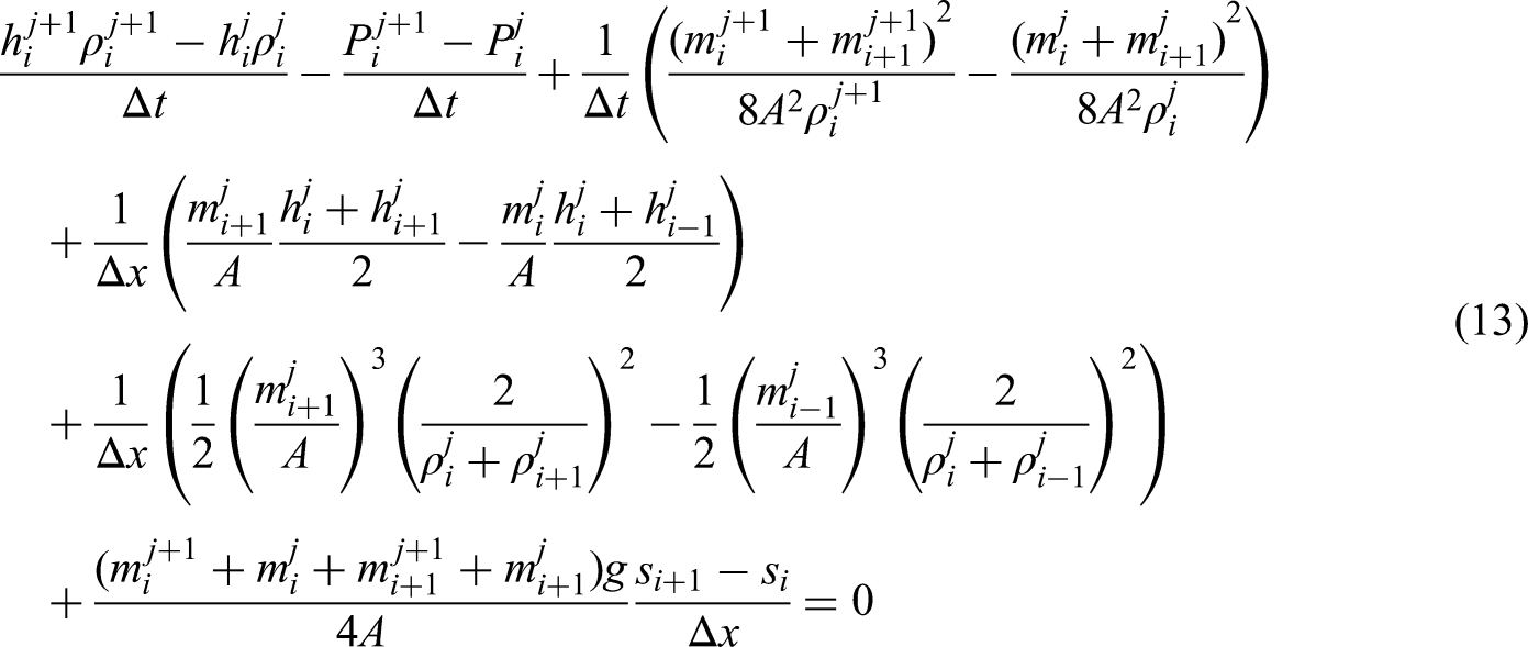
\begin{aligned} \frac{h_{i}^{j + 1} ρ_{i}^{j + 1} - h_{i}^{j} ρ_{i}^{j}}{Δ t} - \frac{P_{i}^{j + 1} - P_{i}^{j}}{Δ t} + \frac{1}{Δ t} (\frac{{(m_{i}^{j + 1} + m_{i + 1}^{j + 1})}^{2}}{8 A^{2} ρ_{i}^{j + 1}} - \frac{{(m_{i}^{j} + m_{i + 1}^{j})}^{2}}{8 A^{2} ρ_{i}^{j}}) \\ + \frac{1}{Δ x} (\frac{m_{i + 1}^{j}}{A} \frac{h_{i}^{j} + h_{i + 1}^{j}}{2} - \frac{m_{i}^{j}}{A} \frac{h_{i}^{j} + h_{i - 1}^{j}}{2}) \\ + \frac{1}{Δ x} (\frac{1}{2} {(\frac{m_{i + 1}^{j}}{A})}^{3} {(\frac{2}{ρ_{i}^{j} + ρ_{i + 1}^{j}})}^{2} - \frac{1}{2} {(\frac{m_{i - 1}^{j}}{A})}^{3} {(\frac{2}{ρ_{i}^{j} + ρ_{i - 1}^{j}})}^{2}) \\ + \frac{(m_{i}^{j + 1} + m_{i}^{j} + m_{i + 1}^{j + 1} + m_{i + 1}^{j}) g}{4 A} \frac{s_{i + 1} - s_{i}}{Δ x} = 0 \end{aligned}

(13)

Based on the above functions, the inherent limitation of the FVM with collocated grids can be further discussed. A key issue lies in the discretization of temperature-related source terms in the energy equation, as expressed below:

\frac{4 K (T_{i}^{j} + T_{i}^{j + 1} + T_{i + 1}^{j} + T_{i + 1}^{j + 1} - 4 T_{U})}{d}

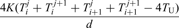
In this formulation, the energy equation only computes the average temperature values at adjacent nodes, meaning that spatial oscillations in the temperature field remain undetected by the discrete equation system. Once initiated, these oscillations persist and propagate, leading to the development of a checkerboard pattern in the temperature distribution. This unphysical pattern subsequently affects the computation of other flow variables through thermo-physical property coupling. In the case of supercritical CO₂, the strong temperature sensitivity of fluid properties intensifies system non-linearities, making such temperature oscillations particularly prone to arising under collocated grid frameworks.

However, with the application of staggered grids, the storage locations of the temperature and velocity variables are offset by half a grid spacing. The direct node value of the temperature T_i^j and T_i^j⁺¹, rather than its interpolated average, is employed in the energy equation, as demonstrated in equation (13). This approach fundamentally resolves the issue of decoupling between temperature and velocity in the discretization.

Boundary conditions

Boundary conditions must be defined at the inlet and/or outlet for all time steps to ensure that the system of equations is mathematically closed. During valve closure in a shutdown scenario, the terminal end of the pipeline applies a valve boundary condition, while the starting end uses a flow rate boundary condition. When the valve opening decreases below 1%, both ends switch to zero-flow-rate boundary conditions. Throughout the shutdown process, the fluid temperature decreases based on the energy equation, governed by heat transfer with the surroundings.

Valve boundary conditions

The thermo-hydraulic behavior of the valve component is modeled using its flow characteristic curve. Under normal operating conditions, the fluid entry node is defined as the valve front, and the exit node as the valve rear. A positive flow velocity corresponds to higher pressure at the valve front than at the rear, while the opposite holds for negative flow. Therefore, the pressure drop across the valve is calculated with the below equation:

P_{1} - P_{2} = \frac{Q | Q | ρ}{C_{v}^{2} ρ_{water}}

(14)

where P₁ and P₂ are the pressures at the valve front and rear, respectively, Pa; Q is the volumetric flow rate at the standard condition, m³·h⁻¹; ρ is the fluid density under local condition, kg·m⁻³; ρ_water is the water density, kg·m⁻³; and C_v is the valve flow coefficient, interpolated from the valve characteristic curve based on valve opening.

The temperature drop across the valve is calculated with the below equation:

T_{1} - T_{2} = μ_{JT} (P_{1} - P_{2})

(15)

where T₁ and T₂ are the temperatures at the valve front and rear, respectively, K and μ_JT is the J–T coefficient, K·Pa⁻¹.

Dirichlet boundary conditions

The Dirichlet boundary condition (i.e. fixed-value constraint) directly assigns values to state variables at pipeline boundaries. During shutdown scenarios, a flow rate boundary condition is applied at the pipeline inlet. Following complete valve closure, a flow rate condition of m = 0 is enforced at the downstream end. The relationship between these conditions and the state variables in the discrete formulation is given by below equations:

m_{0}^{j} = m_{S}^{j}

(16)

m_{N_{x}}^{j} = m_{E}^{j}

(17)

where subscripts denote spatial nodes, while superscripts j indicate time nodes; S represents the start point of the pipeline; and E denotes the end point of the pipeline, with m_S and m_E denoting known boundary conditions.

Self-adaptive time step

Compared to natural gas, CO₂ fluid displays a stronger dependence of its physical properties on temperature and pressure. If the time-step size is too large to accurately capture the rapidly varying flow conditions, the numerical solution may become non-convergent or exhibit oscillations.

Therefore, adaptive time-stepping is required to balance computational efficiency and accuracy. While conventional methods typically adjust the time step based on error estimation (Söderlind, 2002; Söderlind and Wang, 2006), the proposed scheme actively detects flow instability onset and reduces time steps during rapid state transitions to accurately capture water hammer peaks. The proposed algorithm dynamically optimizes step sizes by evaluating flow transition intensity. Additionally, minimum and maximum time-step sizes are specified as Δt_min and Δt_max, respectively.

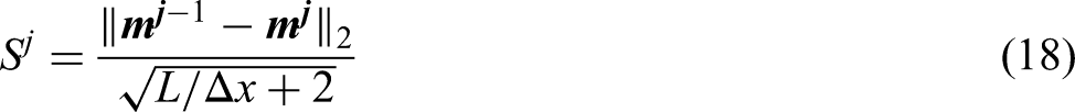
The pipeline flow fluctuations under transient conditions necessitate using the inter-step m-difference as a state-change indicator. The instantaneous variation intensity S^j is defined as below:

S^{j} = \frac{‖ m^{j - 1} - m^{j} ‖_{2}}{\sqrt{L / Δ x + 2}}

(18)

where L/

Δ

x + 2 is the dimension of the flow rate vector m ^j ;

\sqrt{L / Δ x + 2}

is a normalization factor introduced to eliminate the effects of discrete grid numbers.

The adaptive time-stepping strategy operates as follows:

Perform a tentative simulation at time step j with the proposed step size Δt^j. Then go to step (b).

Compute the flow state variation magnitude S^j with equation (18). The time-step size for either the current step j or the next step j + 1 is adjusted based on the value of S^j, as specified in the below equation:

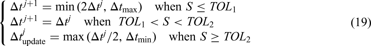
{\begin{matrix} Δ t^{j + 1} = min (2 Δ t^{j}, Δ t_{max}) when S \leq T O L_{1} \\ Δ t^{j + 1} = Δ t^{j} when T O L_{1} < S < T O L_{2} \\ Δ t_{update}^{j} = max (Δ t^{j} / 2, Δ t_{min}) when S \geq T O L_{2} \end{matrix}

(19)

When S^j ≤ TOL₁, indicating minor flow state variation between steps j and j + 1, the next time step is set to double the current step size or the maximum time step. Then go to step (c).

When TOL₁ < S^j < TOL₂, the flow state fluctuation amplitude is regarded as compatible with the simulation step size, thus maintaining identical step sizes for j and j + 1. Then go to step (c).

When S^j ≥ TOL₂, significant flow state variation implies the time step Δt^j is too large; recompute the current step with an updated Δt^j_update. Then go back to step (a).

(c)Go to time step j + 1 with the proposed step size Δt^j⁺¹.

The values of TOL₁ and TOL₂ are determined through fixed-step trial simulations, which are illustrated using a simulation of a pipeline in the Case study section.

The thermo-hydraulic simulation for supercritical CO₂ pipelines is modeled in Python, with the Newton–Raphson method provided by the Fsolve to solve the iterative equations.

Case study

The proposed model is used to simulate CO₂ pipeline shutdown scenarios and validated against OLGA results. Thus, water hammer analysis is conducted with the proposed model.

Pipeline parameters

A CO₂ pipeline transport system is simulated as a case study, which is illustrated in Figure 2. The pipeline has a total length of 78 km, a pipe diameter of 304.8 mm, a wall thickness of 3.15 mm, and an internal surface roughness of 0.05 mm. The ambient temperature is 13.1 °C with an overall heat transfer coefficient of 15 W·m⁻²·K⁻¹. Fluid composition details are provided in Table 1.

Figure 2.

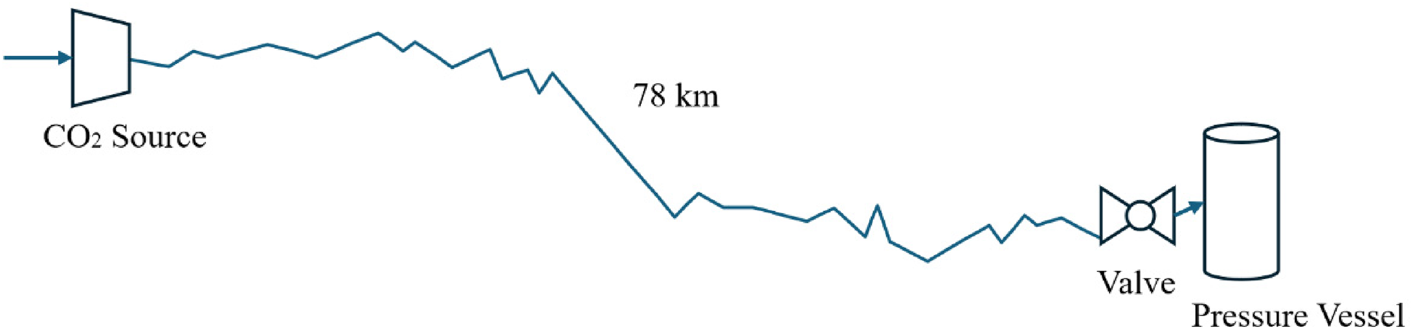
Diagram of the CO₂ pipeline system.

Table 1.

Composition of CO₂ fluid with impurities.

Component	CO₂	N₂	CH₄	H₂S	H₂O
Mole fraction (%)	97	0.8	1.9	0.02	0.01

A ball valve is installed at the pipeline outlet and connected to a pressure tank. The maximum flow coefficient of the valve is C_Vmax = 5000. The relative flow coefficient is defined as C_V/C_Vmax. The relationship between the relative flow coefficient and valve opening position is shown in Figure 3.

Figure 3.

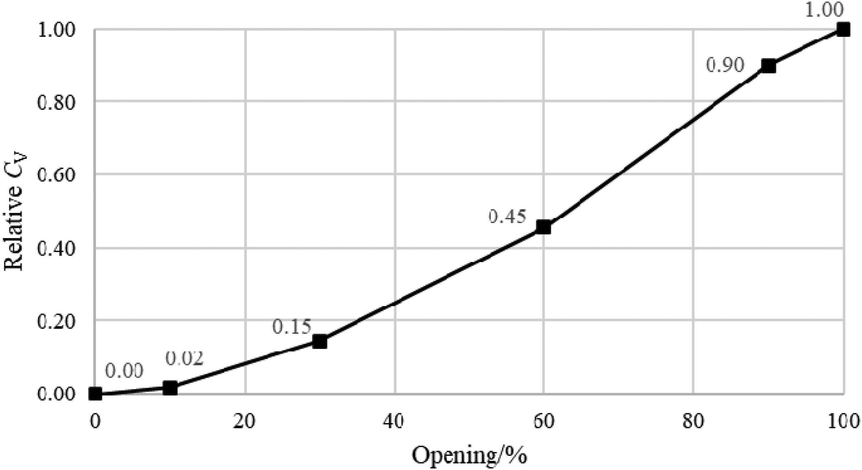
Relative C_V versus opening curve of the shutdown valve at the outlet of the pipeline.

Simulation results

Model validation is performed using OLGA simulation software, with fluid properties calculated with the GERG-2008 equation in Multiflash. The computational accuracy for pressure, temperature, flow rate, and density distributions along the pipeline is verified. For the shutdown scenario simulations in both OLGA and the proposed models, corresponding initial pre-shutdown conditions are established through steady-state simulations.

Spatial convergence analysis was conducted to identify an optimal fixed spatial step size of 500 m. This discretization preserves numerical accuracy while reducing computational load by 63% compared to a 250 m step size. Additionally, adaptive time-stepping (Δt ∈ [0.1 s, 60 s]) was employed to maintain computational efficiency during transient simulations.

Steady-state initial conditions

Steady-state simulation results from the FVM, improved FVM, and OLGA models are presented and compared. All three models yield highly consistent and stable computational outcomes under both supercritical and dense-phase conditions. The initial flow rate is 1 million tons per year (33.3 kg·s⁻¹), with a fluid temperature of 33 °C. The pressure in the vessel behind the valve remains constant at 8600 kPa, which is approximately 1.1 times the critical pressure (Figure 4).

Figure 4.

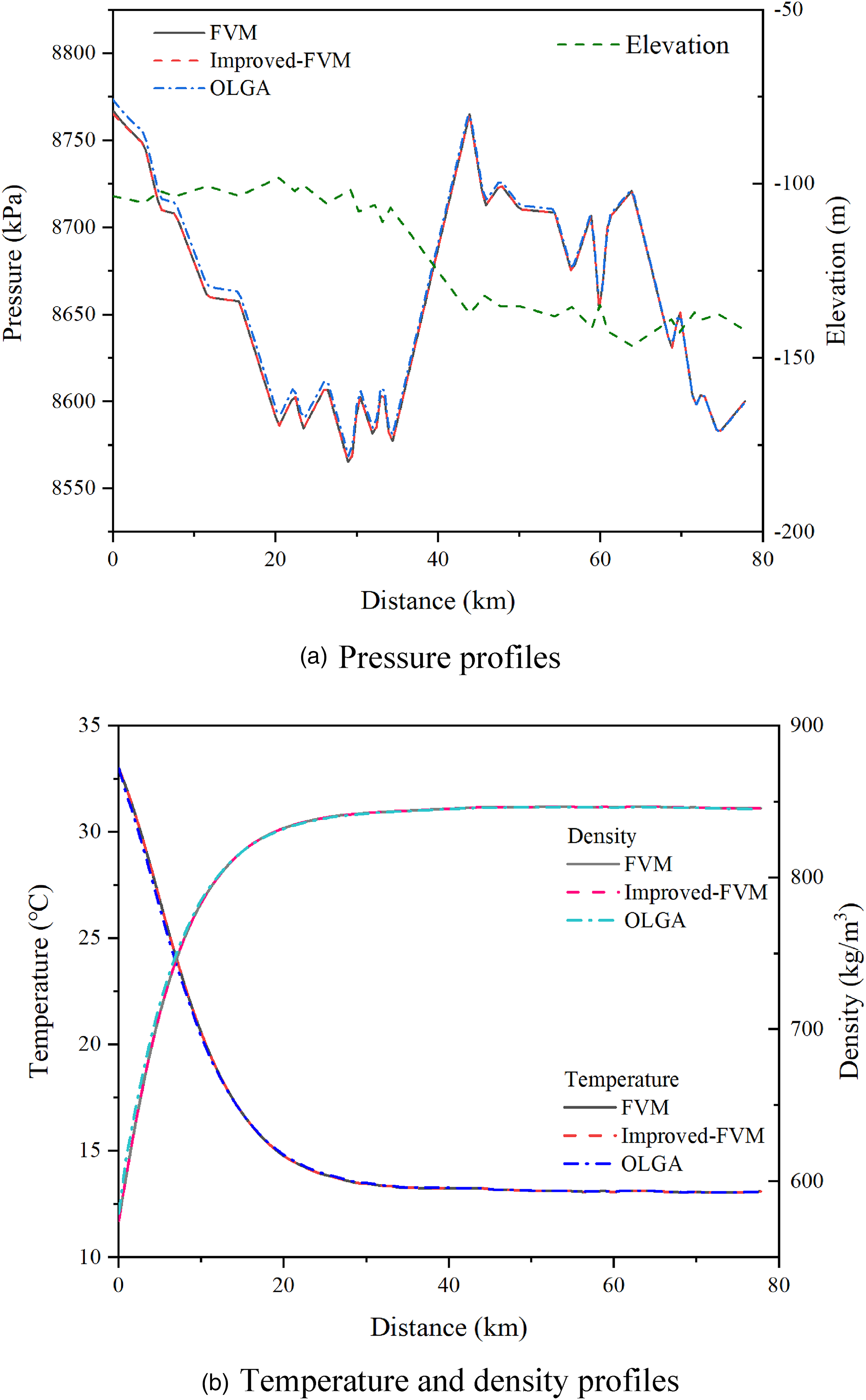
Steady-state profiles of (a) pressure and (b) temperature and density along the pipeline simulated with FVM, improved FVM, and OLGA. All three simulators demonstrate strong agreement in steady-state simulation. FVM: finite volume method.

Transient simulation results

Transient simulations were initialized using the steady-state solutions obtained in the previous section and involved a linear valve closure event over 12 s (from 100% opening to 0%). The conventional FVM shows significant temperature oscillations at about 19 min, then propagating hydraulic errors. In contrast, the staggered-grid-enhanced FVM algorithm effectively suppresses these numerical instabilities. The temperature and flow profiles at this time step for both the conventional and improved FVM methods are compared in Figure 5.

Figure 5.

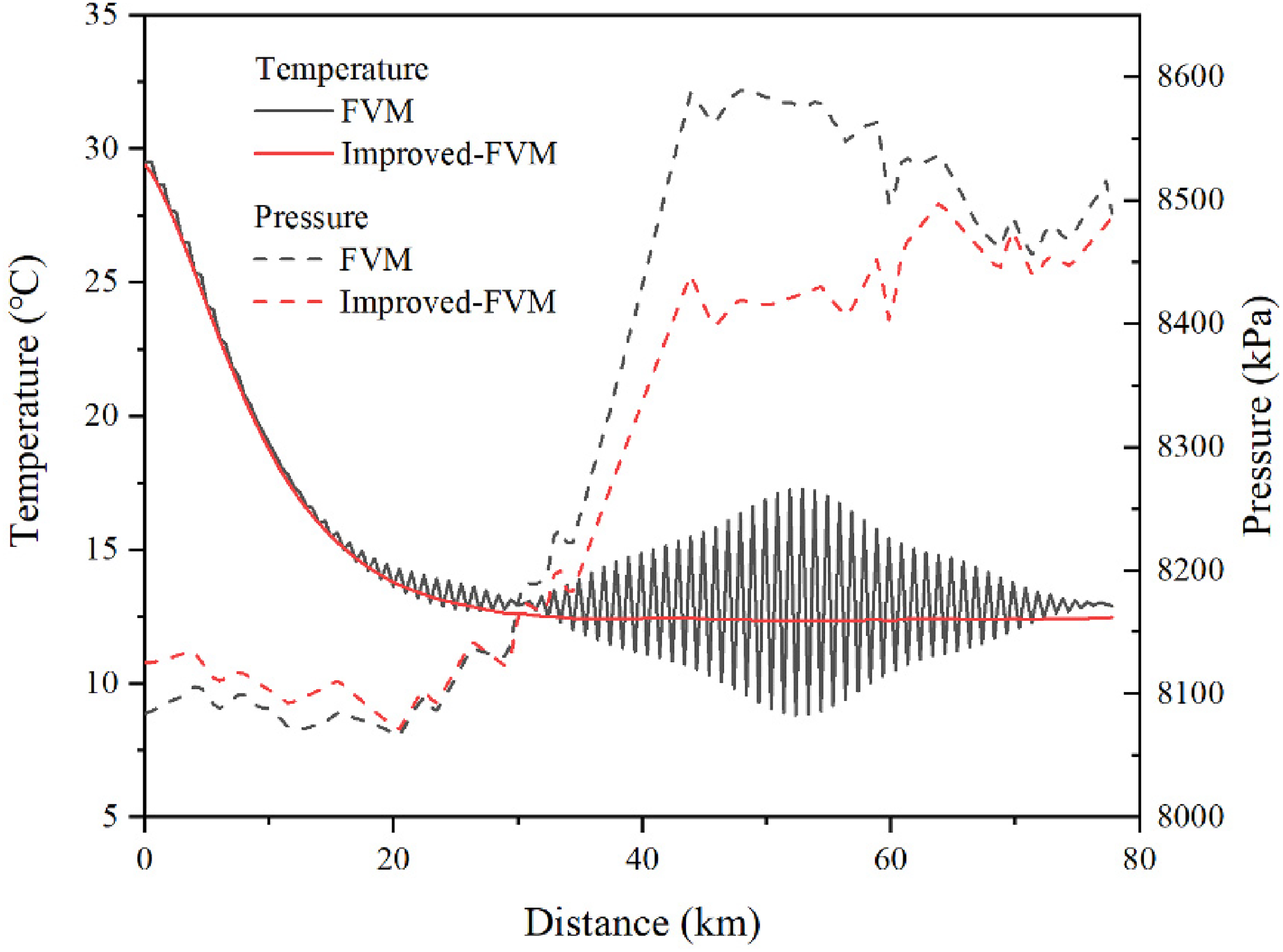
Comparison of temperature and pressure profiles of the FVM and improved FVM model during pipeline shutdown (t = 19 min). The original FVM produces unphysical oscillations in its temperature prediction. In contrast, the improved FVM yields a stable solution, confirming the enhanced numerical stability and accuracy of the improved FVM with staggered grids. FVM: finite volume method.

Reducing the time step can mitigate but not eliminate temperature oscillations in the conventional FVM, as this is an underlying limitation of the collocated grids. When the time step is reduced to 5 s, oscillations persist at the pipeline outlet by the 19th minute, as shown in Figure 6(a), and continue to propagate. Even with a time step of 0.1 s, these oscillations still remain, as evidenced in Figure 6(b). In contrast, the present improved FVM based on a staggered grid completely eliminates this issue.

Figure 6.

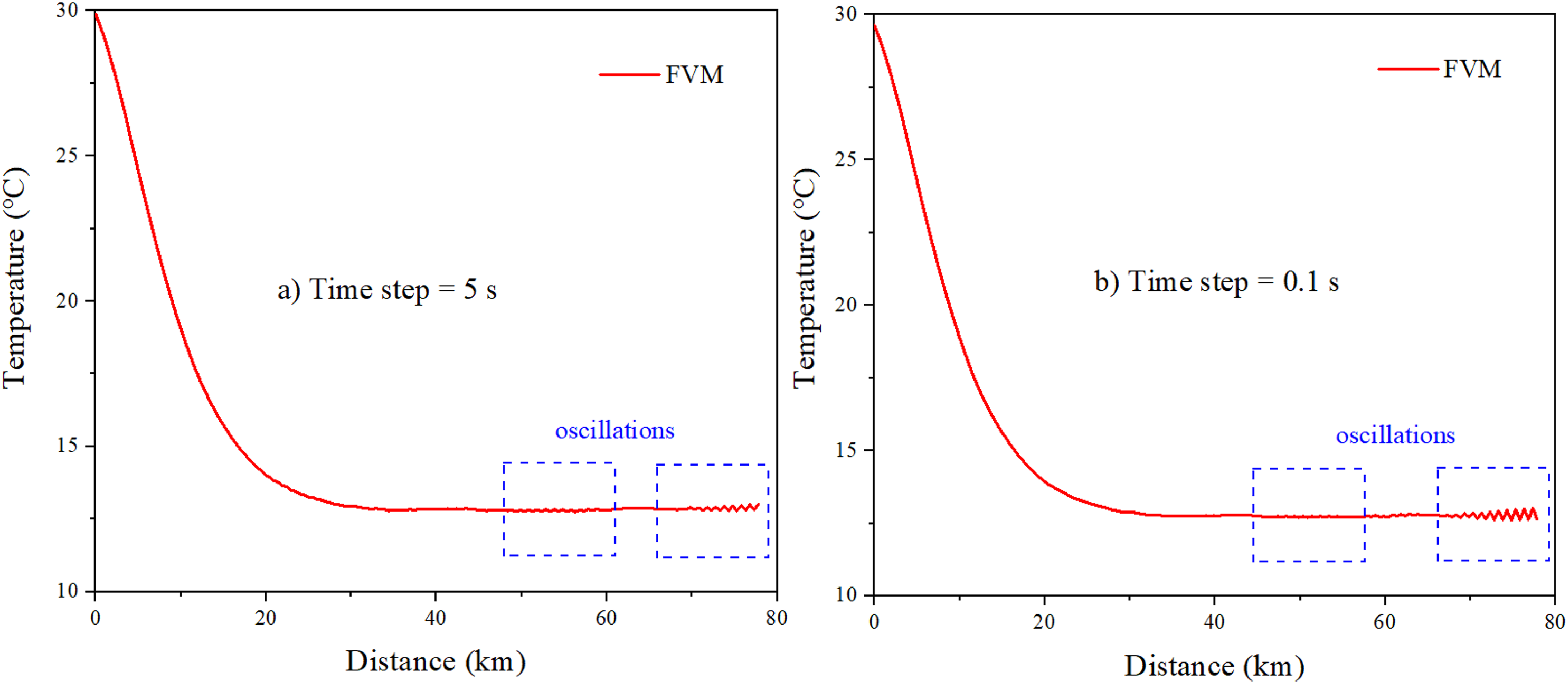
Temperature oscillations with the original FVM model during pipeline shutdown under different time steps: (a) 5 s and (b) 0.1 s. Reducing the time step to 5 s or 0.1 s can mitigate the numerical oscillations but cannot eliminate them, indicating an inherent instability in the original model formulation. FVM: finite volume method.

An adaptive time-step adjustment strategy is applied in the transient simulation. TOL₁ and TOL₂ represent the critical thresholds for the variation amplitude of the flow state, with TOL₁ ≤ TOL₂. Setting both values too large increases the computational time step, which may lead to numerical oscillations and/or reduced accuracy. Conversely, if the values are set too small, the computational time step decreases, resulting in excessive resource consumption.

A sensitivity analysis is conducted to compare the computational results under different sets of TOL₁ and TOL₂. Since the flow state stabilizes after 30 min and the time step under various cases has reached 60 s, only the results from the first 30 min are compared. The variations of the pipeline outlet pressure under different cases are shown in Figure 7. The analysis includes the following cases:

TOL₁ = 4, TOL₂ = 8: The results exhibit oscillations.

TOL₁ = 2, TOL₂ = 4: The results deviate significantly with low computational accuracy.

TOL₁ = 0.5, TOL₂ = 1: The results meet both accuracy and stability requirements, taking 212 steps and 403 s to simulate a 30-min shutdown process.

TOL₁ = 0.2, TOL₂ = 0.5: The results satisfy the accuracy requirements but are computationally intensive, taking 717 steps and 1286 s to simulate a 30-min shutdown process.

Figure 7.

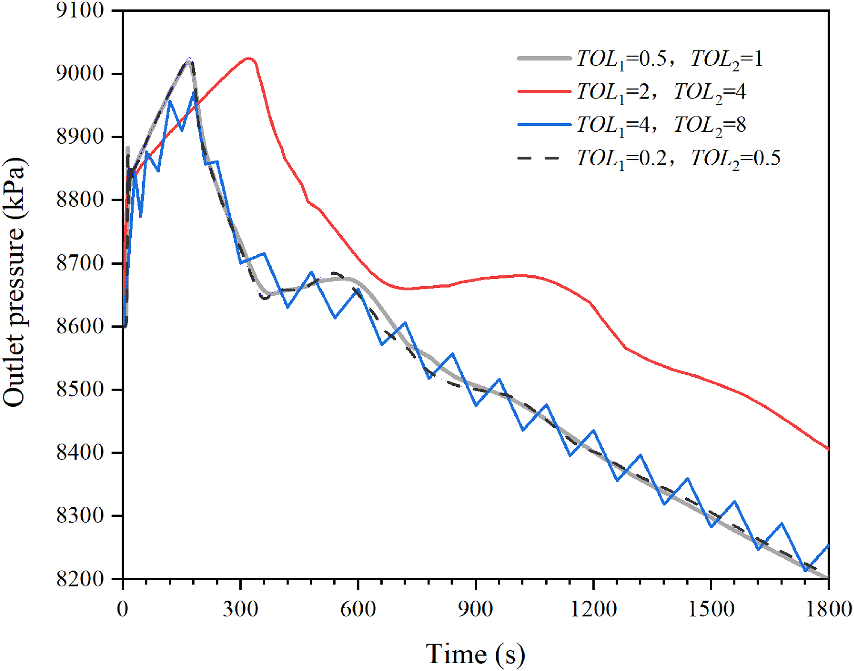
Sensitivity of simulation results to the adaptive time-step thresholds values (TOL₁ and TOL₂) in the 30-min shutdown simulation. The computational results progressively converge with decreasing TOL₁ and TOL₂.

Consequently, the thresholds TOL₁ = 0.5 and TOL₂ = 1 are selected for time-step adjustment using equation (17), considering simulation accuracy and computational cost. Over the 12-h simulation period, the temporal evolution of step sizes demonstrates progressive growth toward Δt_max as flow conditions asymptotically stabilize, as shown in Figure 8.

Figure 8.

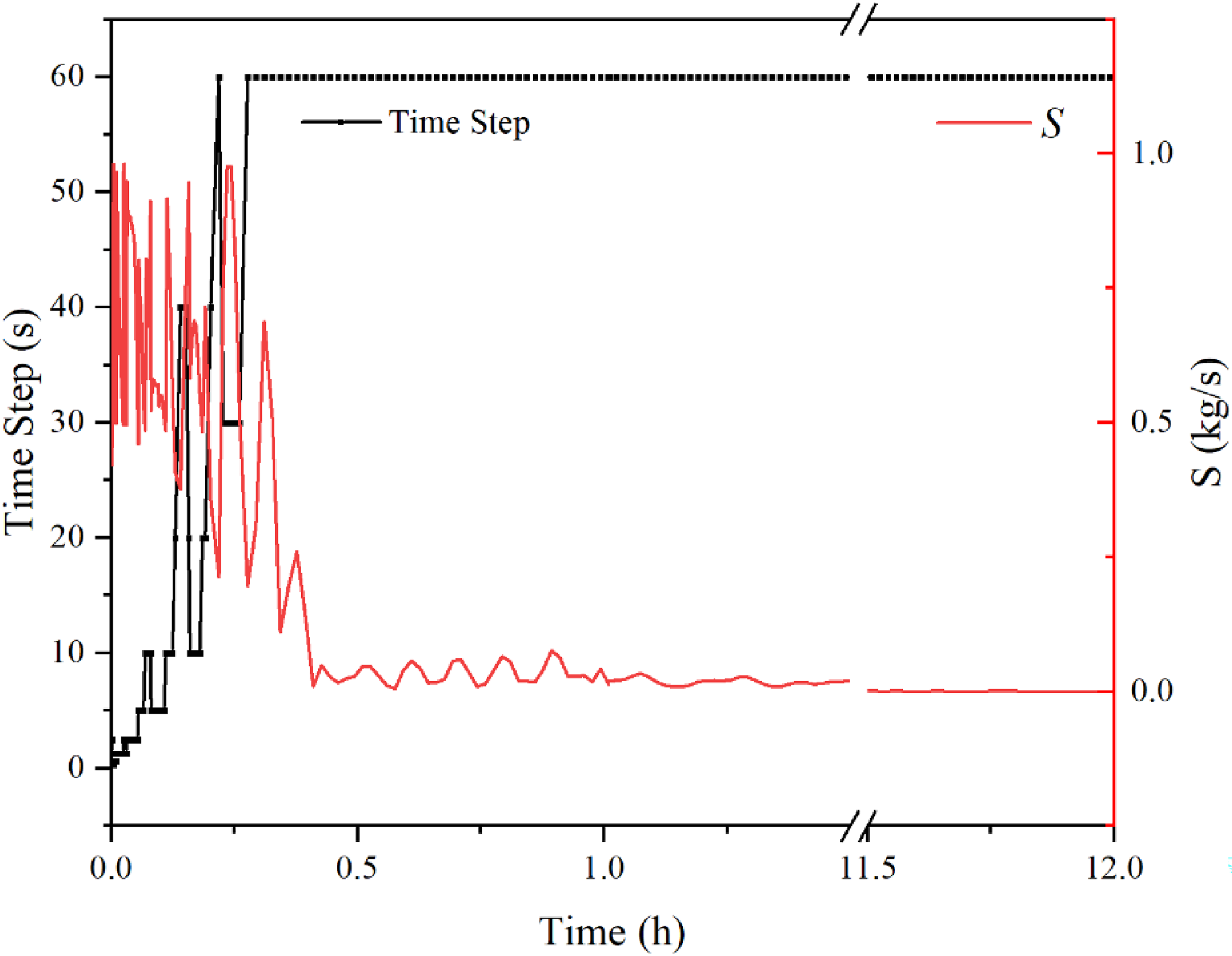
Evolution of the time step during the transient pipeline shutdown simulation. The time step was adaptively increased to a predefined maximum as the flow field stabilized.

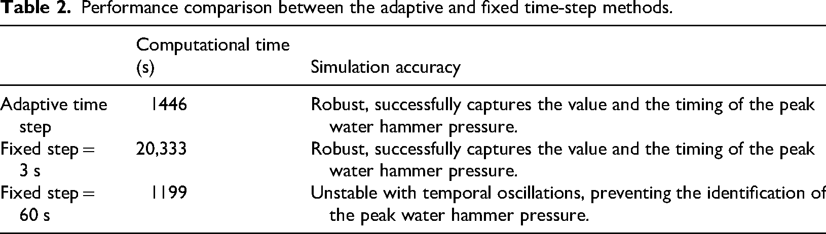
The adaptive time-step method significantly enhanced computational efficiency while maintaining accuracy. Compared to a fixed time step of 3 s, the adaptive approach reduced the number of iterations and the overall computational time by 94% in a 12-h shutdown simulation. In contrast, while a 60-s fixed time step performs a comparable computational cost to the adaptive method, it is too coarse to resolve the rapid transients of the initial valve closure, resulting in pronounced numerical oscillations in the results (Table 2).

Table 2.

Performance comparison between the adaptive and fixed time-step methods.

	Computational time (s)	Simulation accuracy
Adaptive time step	1446	Robust, successfully captures the value and the timing of the peak water hammer pressure.
Fixed step = 3 s	20,333	Robust, successfully captures the value and the timing of the peak water hammer pressure.
Fixed step = 60 s	1199	Unstable with temporal oscillations, preventing the identification of the peak water hammer pressure.

Based on the above analysis, the improved FVM algorithm offers better computational stability in transient simulation, while the adaptive time step can accommodate fluctuations under pipeline conditions. Therefore, all subsequent studies are conducted using the improved FVM algorithm with an adaptive time step.

First, the simulation results from the improved FVM are benchmarked against OLGA. The axial temperature distributions along the pipeline at 0 min, 5 min, 30 min, 90 min, and 12 h are presented in Figure 9.

Figure 9.

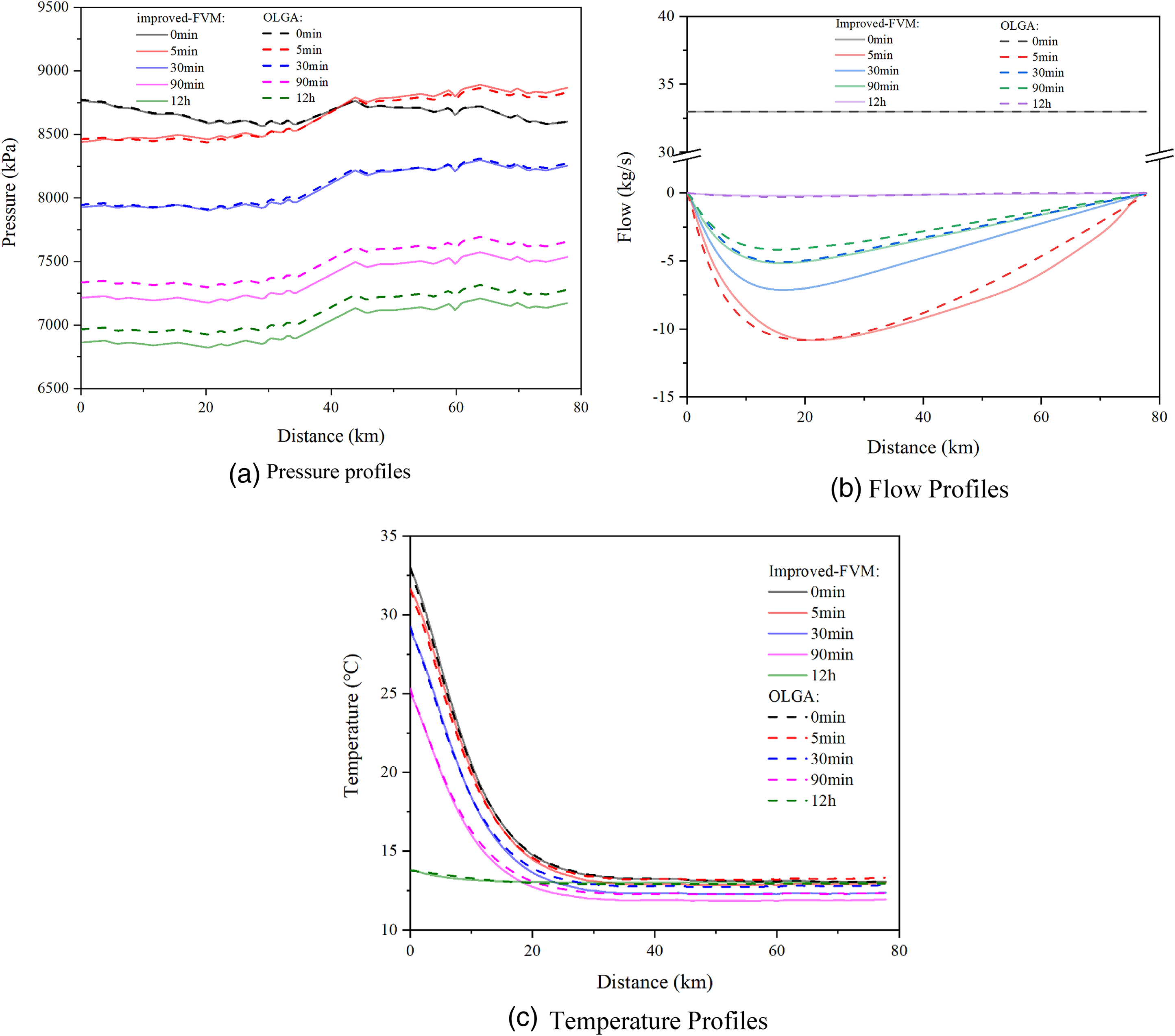
Model validation of the improved FVM against OLGA for CO₂ pipeline shutdown scenario. Comparisons of (a) pressure, (b) flow rate, and (c) temperature profiles along the pipeline at 0, 5, 30, 90, and 720 min. Results from the developed model (solid lines) show strong agreement with those from the OLGA simulator (dashed lines). The consistent match across the parameters confirms the reliability of the proposed model in predicting the complex thermo-dynamic behavior of CO₂ during transient pipeline operations. FVM: finite volume method.

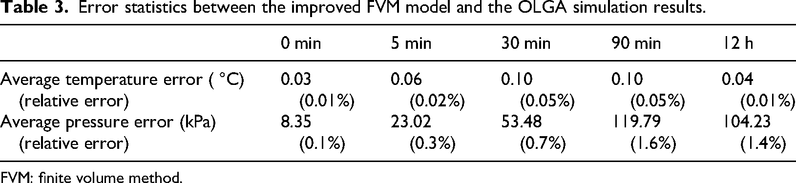
Simulation results from both OLGA and the improved FVM model show a consistent decrease in pressure and temperature. The average errors in the along-pipeline distributions of pressure and temperature between the two models per time step are quantified in Table 3. The maximum average temperature and pressure errors are 0.05% and 1.6%, respectively, indicating that the improved FVM model is in excellent agreement with the OLGA results.

Table 3.

Error statistics between the improved FVM model and the OLGA simulation results.

	0 min	5 min	30 min	90 min	12 h
Average temperature error ( °C) (relative error)	0.03 (0.01%)	0.06 (0.02%)	0.10 (0.05%)	0.10 (0.05%)	0.04 (0.01%)
Average pressure error (kPa) (relative error)	8.35 (0.1%)	23.02 (0.3%)	53.48 (0.7%)	119.79 (1.6%)	104.23 (1.4%)

FVM: finite volume method.

During the shutdown process, progressive cooling of the fluid occurs when the ambient temperature is lower than that of the fluid. Supercritical/dense-phase CO₂ exhibits a high sensitivity of density to temperature variations. The temperature decline at the upstream end leads to a reduction in pressure below that of the downstream section, resulting in a reversal of flow direction from forward to backward until the flow eventually stabilizes at zero. As a result, the pressure profile decreases continuously throughout the shutdown process. Ultimately, the pressure distribution along the pipeline becomes elevation-dependent under stagnant conditions.

The results emphasize the critical importance of monitoring thermally-induced pressure drop during shutdown to prevent potential phase transitions. The fluid in the case transitions from a supercritical phase to a dense phase and finally to a liquid phase. It is important to note that the fluid should be prevented from reaching the gas phase during the shutdown process. Phase transitions between supercritical/dense/liquid phases and the gas phase may cause severe pressure fluctuations in the pipeline, affecting the structural safety of the pipeline. Therefore, it is recommended to simulate the shutdown process before executing the operation, and to control the fluid's phase state by regulating the pressure inside the pipeline before or during shutdown.

For the 78-km CO₂ pipeline case study, a spatial step of 500 m discretizes the pipeline into 157 primary grids and 156 velocity grids. The discretization resulted in a system of transient simulation equations with a size of 472. The simulation cost an average computational time of 1.6 s per time step, with a duration of about 24 min for a 12-h shutdown simulation (CPU: AMD Ryzen 7 5800H, 3.20 GHz; RAM: 16.0 GB). The computational speed is generally acceptable for engineering applications.

However, the computational cost exhibits a strong dependence on the equation system size. For instance, when the pipeline length is doubled to 156 km while maintaining the same space step, the size of the equation system nearly doubles to 937, and the computational time per step increases to 7.2 s. A further increase in length to 234 km led to a sharp rise in the per-step simulation time to 39.2 s. This trend demonstrates a non-linear growth in computational cost with increasing system scale. Therefore, for the simulation of long-distance pipeline systems, increasing the spatial step size can be a practical strategy to maintain computational time within feasible engineering limits while retaining acceptable accuracy.

Water hammer analysis

Theoretical calculations of water hammer pressure and wave speed are performed using analytical formulas to establish two-way validation with simulation results. This approach involves applying theoretical formulas to interpret the simulation outcomes, while utilizing simulation to verify whether conventional water hammer equations—typically applied to liquid pipelines—remain valid for supercritical/dense-phase CO₂ systems.

The water hammer pressure can be calculated with the Joukowsky equation as shown below:

Δ P = ρ \cdot a \cdot Δ v

(20)

where ΔP is the water hammer pressure, Pa; ρ denotes fluid density, kg·m⁻³; a denotes pressure wave speed, m·s⁻¹; and Δv is the change in fluid velocity, m·s⁻¹.

The pressure wave speed is calculated with the below equation:

a = \frac{c}{\sqrt{1 + K d / E e}}

(21)

where c is the local sound speed, m·s⁻¹; K denotes the bulk modulus of the fluid, Pa; d is the inner diameter of the pipe, m; e is the pipe wall thickness, m; and E is the pipe elastic modulus, Pa.

Derived from the fundamental acoustic velocity definition, the computational formulation for sound speed in supercritical CO₂ is provided in the below equation: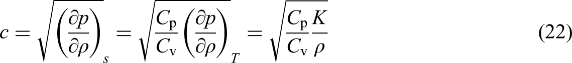

c = {\sqrt{(\frac{\partial p}{\partial ρ})}}_{s} = {\sqrt{\frac{C_{p}}{C_{v}} (\frac{\partial p}{\partial ρ})}}_{T} = \sqrt{\frac{C_{p}}{C_{v}} \frac{K}{ρ}}

(22)

where C_p and C_v are isobaric heat capacity and isochoric heat capacity, respectively, J·mol⁻¹·K⁻¹.

For conventional liquid pipelines, sound speed is calculated with equation (23), since C_p/C_v is approximately 1. However, equation (23) is invalid for supercritical/dense-phase CO₂ fluid. The original equation (22) must be applied instead:

c_{l} = \sqrt{K / ρ}

(23)

The steel pipeline has an elastic modulus of 2.06 × 10¹¹ Pa. The thermo-physical properties of the CO₂ fluid are calculated using GERG-2008 and equations (21) and (22). Parameters related to water hammer at the pipeline inlet and outlet are provided in Table 4.

Table 4.

Physical parameters of CO₂ fluid under operating conditions.

Position	ρ (kg·m⁻³)	K (Pa)	C_p (J·mol⁻¹·K⁻¹)	C_v (J·mol⁻¹·K⁻¹)	c (m·s⁻¹)	a (m·s⁻¹)
Start-point status (P = 8763 kPa, T = 33 °C)	574.1	3.7 × 10⁶	390.3	49.3	227.4	225.2
End-point status (P = 8600 kPa, T = 13 °C)	846.0	6.7 × 10⁷	116.3	41.0	472.5	468.8
Average status (P = 8661 kPa, T = 15 °C)	831.7	5.9 × 10⁷	120.3	41.1	454.3	449.9

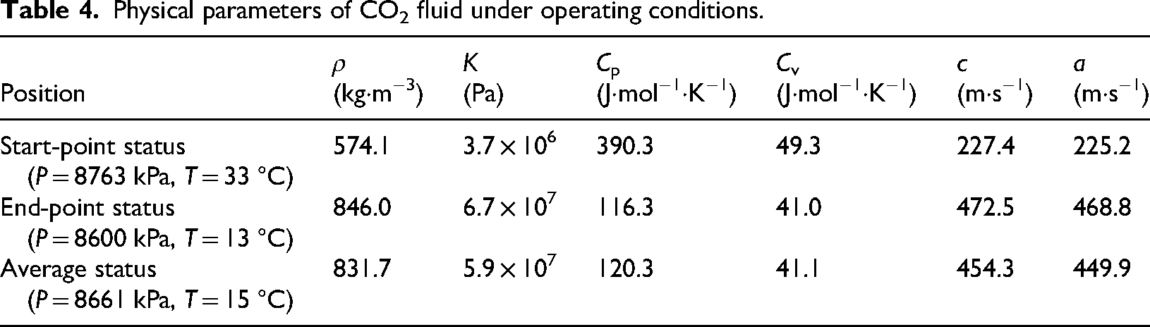
Based on equation (20), the direct water hammer pressure generated at the terminal valve closure is 221 kPa, while the decompression wave magnitude is 106 kPa at the inlet. Compared to pure liquid pipelines (e.g. oil or water), the water hammer pressure in supercritical/dense-phase CO₂ is approximately one-fourth to one-tenth that magnitude. Using the average water hammer wave speed of 449.9 m·s⁻¹, the propagation time from pipeline outlet to inlet t_wh is calculated as follows:

t_{wh} = L / a = 78, 000 / 449.9 = 173.4 s

The water hammer analysis is also performed based on the simulation results, which allows for cross validation with the formula-based calculation results. Figure 10 shows inlet and outlet pressure variations during shutdown. The pressure curves of the improved FVM model and OLGA show errors within 160 kPa (2.2%). Analysis of water hammer pressures at both pipeline ends shows consistent results between the proposed model and OLGA simulations, validating the model's accuracy in predicting water hammer pressure.

Figure 10.

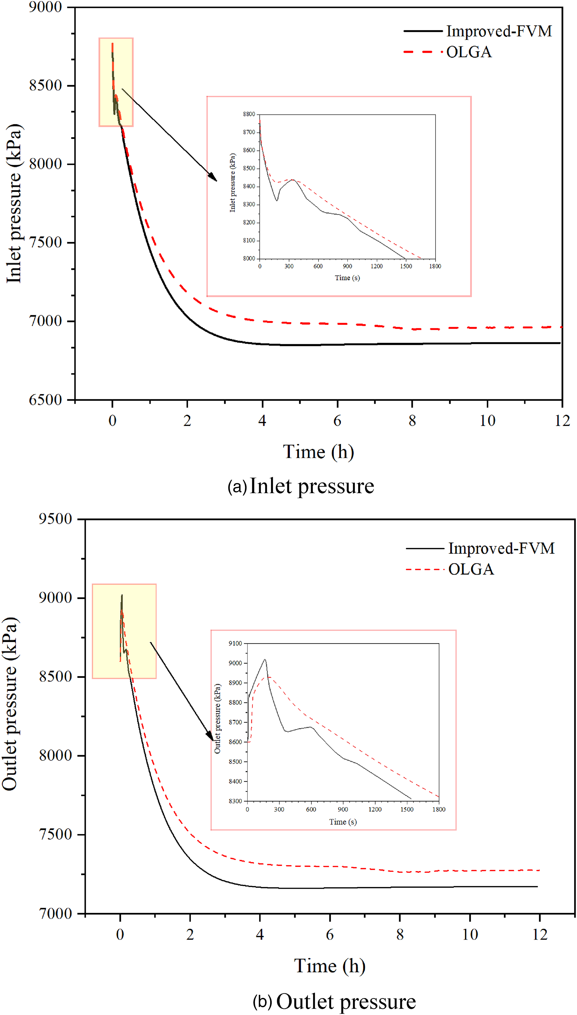
Transient pressure response at the (a) inlet and (b) outlet during pipeline shutdown. The maximum water hammer pressure at the inlet reaches 8437 kPa at 350 s, whereas a peak pressure of 9020 kPa occurs at the outlet at 165 s. The timing of these peaks is consistent with theoretical wave speed predictions. The observed water hammer pressure, however, deviates from theory due to physical mechanisms: wave attenuation reduces the peak pressure at the inlet, while additional packing pressure amplifies it at the outlet.

The pressure variation at the pipeline inlet, as shown in Figure 9(a), can be divided into three distinct stages:

1. Initially, the inlet pressure decreases in response to the reduction in inlet flow rate at the onset of shutdown.

2. Subsequently, a compression wave arrives at approximately 160 s, which aligns well with the theoretical wave propagation time (t_wh) from the pipeline outlet to the inlet. The water hammer pressure peak occurs at 350 s (0.1 h), with the inlet pressure reaching its maximum of 8437 kPa.

The observed peak water hammer pressure at the pipeline inlet is 112 kPa, significantly lower than the theoretical value of 221 kPa. This discrepancy can be attributed to the higher elastic modulus of CO₂ than that of the regular liquid, which causes wave attenuation during propagation. In addition, the superposition between the incoming compression wave and the decompression wave traveling downstream from the inlet further reduces the pressure peak.

3. Finally, as the fluid temperature gradually decreases to ambient levels, the inlet pressure continues to decline until a steady state is reached.

The pressure variation at the front of the outlet valve, as shown in Figure 9(b), can be explained as two stages:

First, the pressure at the valve front continuously rises in duration 0–165 s (0–0.05 h), reaching a maximum water hammer pressure of 9020 kPa. The simulated water hammer pressure near the valve is 380 kPa, which exceeds the theoretical value of 221 kPa. This discrepancy arises because the valve is subjected not only to direct water hammer effects but also to an additional packing pressure. The packing pressure is generated as the fluid continues to move downstream, driven by both the hydraulic pressure difference. Consequently, it is recommended to employ shutdown simulations for accurate water hammer assessment, as the Joukowsky formula tends to underestimate the pressure at the pipeline outlet while overestimating it at the inlet.

Following this, a decompression wave originating upstream arrives at 165 s. Then the pressure then gradually decreases due to the cooling effect until it eventually stabilizes.

The valve closure time influences the magnitude of water hammer pressure by reducing the packing pressure, while the direct water hammer pressure remains unchanged. The relationship between water hammer pressure at the valve front and closure time under different valve closure strategies is shown in Figure 11. When the valve closure time is extended by 10 times from 12 to 120 s, the total water hammer pressure decreases by only 20%. It is shown that prolonging the closure time can help reduce water hammer pressure with limited effect. Therefore, for pipeline systems where extending valve closure time proves insufficient, the implementation of dedicated surge protection measures is recommended. Primary alternatives include surge relief valves, which mitigate pressure peaks by diverting a small volume of fluid. The selection of an optimal strategy should be based on a comprehensive evaluation of the system requirements and constraints.

Figure 11.

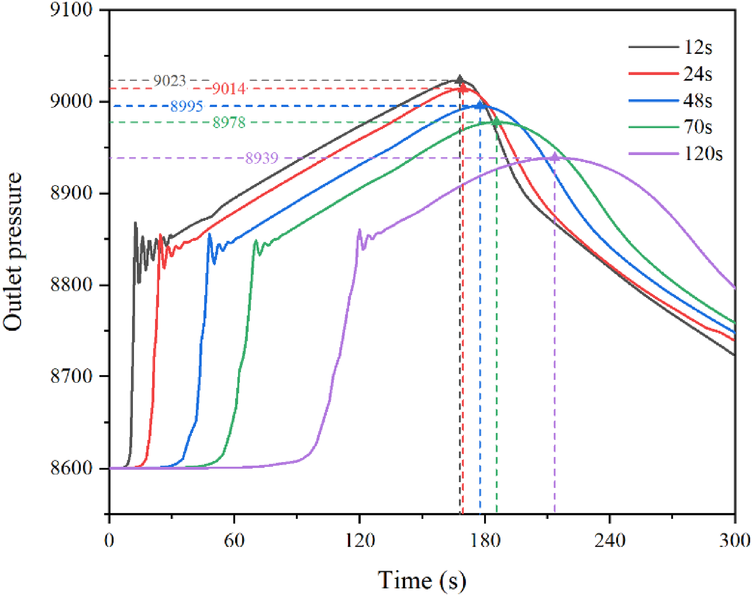
Transient pressure response at the terminal valve at different valve closure times. Increasing the closure time from 12 to 120 s reduces the water hammer pressure by merely 20%, highlighting the practical limitation of relying solely on valve closure time for pressure control.

Conclusions

A modified FVM for simulating supercritical and dense-phase CO₂ pipelines is proposed, which combines a staggered grid arrangement with an explicit differencing scheme for convective terms to eliminate numerical oscillations. An adaptive time-step strategy is introduced to effectively handle rapid state fluctuations. The model is validated under shutdown scenarios while retaining its applicability to normal operating conditions involving variations in pressure, flow rate, and temperature.

A modified FVM for simulating supercritical and dense-phase CO₂ pipelines is proposed, which combines a staggered grid arrangement with an explicit differencing scheme for convective terms to eliminate numerical oscillations. An adaptive temporal resolution strategy is introduced to effectively handle rapid state fluctuations. The model is validated under shutdown scenarios while retaining its applicability to normal operating conditions involving variations in pressure, flow rate, and temperature.

A comparison between the Joukowsky formula and simulation results shows good agreement in predicting the water hammer wave speed in CO₂ pipelines. However, the formula relies on a sound speed equation applicable to supercritical fluids. Simulations further reveal the presence of significant packing pressure upstream of the valve during shutdown. Therefore, simulation-based analysis is necessary for accurate water hammer pressure assessment, as the Joukowsky formula accounts only for direct water hammer effects and yields insufficient estimates under these conditions.

This improved HEM model is proposed to simulate the thermo-hydraulic characteristics of CO₂ pipelines. However, the HEM model neglects interfacial forces, which can introduce significant errors in certain scenarios, such as during leakage or venting. The present methodology provides a foundation for future application to a two-fluid model to address this limitation.

Footnotes

ORCID iD

Yaran Bu

Funding

The authors disclosed receipt of the following financial support for the research, authorship, and/or publication of this article: The research was funded by “Research on Key Technologies and System Integration for Intelligent Production of Floating Deepwater Oil and Gas Production, Storage, and Offloading Units” (2024ZD1403306), a sub-topic of the National Science and Technology Major Project “Key Technologies and Equipment for Dry Production and Processing Platforms in Deepwater Oil and Gas”.

Declaration of conflicting interests

The authors declared no potential conflicts of interest with respect to the research, authorship, and/or publication of this article.

References

Aursand

Hammer

Munkejord

, et al. (2013) Pipeline transport of CO₂ mixtures: Models for transient simulation. International Journal of Greenhouse Gas Control 15: 174–185.

Bielka

Kuczyński

Włodek

, et al. (2024) Risks and safety of CO₂ pipeline transport: A case study of the analysis and modeling of the risk of accidental release of CO₂ into the atmosphere. Energies 17(16): 3943.

Botros

Geerligs

Rothwell

, et al. (2017) Measurements of decompression wave speed in binary mixtures of carbon dioxide and impurities. Journal of Pressure Vessel Technology, Transactions of the ASME 139(2): 1–11.

Brodskyi

Gyrya

Zlotnik

(2025) Simulation of gas mixture dynamics in a pipeline network using explicit staggered-grid discretization. Applied Mathematical Modelling 137(PB): 115717.

Brown

Martynov

Mahgerefteh

, et al. (2014) Modelling the non-equilibrium two-phase flow during depressurisation of CO₂ pipelines. International Journal of Greenhouse Gas Control 30: 9–18.

Diamantonis

Boulougouris

Mansoor

, et al. (2013) Evaluation of cubic, SAFT, and PC-SAFT equations of state for the vapor–liquid equilibrium modeling of CO₂ mixtures with other gases. Industrial and Engineering Chemistry Research 52(10): 3933–3942.

Divahar

Roberts

Mattner

, et al. (2024) Staggered grids for multidimensional multiscale modelling. Computers and Fluids 271(January): 106167.

DNVGL-RP-F104 (2021) Design and operation of carbon dioxide pipelines.

Dong

Jiang

, et al. (2025) Comparative life cycle assessment of CO₂ onshore transport in China: Pipeline or tanker truck? Journal of CO₂ Utilization 94(January): 103057.

10.

Drescher

Fahmi

Aursand

, et al. (2017) Towards a thorough validation of simulation tools for CO₂ pipeline transport. Energy Procedia 114(November 2016): 6730–6740.

11.

El-Kady

Amin

Khan

, et al. (2024) Analysis of CO₂ pipeline regulations from a safety perspective for offshore carbon capture, utilization, and storage (CCUS). Journal of Cleaner Production 439(October 2023): 140734.

12.

ISO 20765-2:2015 (2015) Natural gas—Calculation of thermodynamic properties—Part 2: Single-phase properties (gas, liquid, and dense fluid) for extended ranges of application.

13.

ISO 27913:2016 (2016) Carbon dioxide capture, transportation and geological storage—Pipeline transportation systems.

14.

Kim

Yoon

Lee

(2024) Review on carbon capture and storage (CCS) from source to sink; part 1: Essential aspects for CO₂ pipeline transportation. International Journal of Greenhouse Gas Control 137(September 2023): 104208.

15.

Kunz

Wagner

(2012) The GERG-2008 wide-range equation of state for natural gases and other mixtures: An expansion of GERG-2004. Journal of Chemical and Engineering Data 57(11): 3032–3091.

16.

Wang

, et al. (2025) Thermohydraulic characterization of supercritical and dense-phase CO₂ pipeline transportation with impurities. Journal of Supercritical Fluids 224(January): 106666.

17.

Liu

Wang

Zhang

, et al. (2013) Comparison study on the performances of finite volume method and finite difference method. Journal of Applied Mathematics 2013.

18.

Zhang

, et al. (2024) Numerical simulation of impurity-containing supercritical CO₂ pipeline transport in CCUS. International Journal of Greenhouse Gas Control 138(August): 104236.

19.

Luo

Chirkov

(2021) Calculation of thermodynamic properties of mixtures in two-phase equilibrium. Journal of Physics: Conference Series 2039(1).

20.

Martynov

Zheng

Brown

, et al. (2016) Numerical simulation of CO₂ flows in pipes with phase transition. In: International conference on heat transfer, fluid mechanics and thermodynamics, Costa de Sol, 2016, pp. 1080–1085.

21.

Martynov

Zheng

Mahgerefteh

(2018) Numerical study of the effect of heat transfer on solid phase formation during decompression of CO2 in pipelines. In: MATEC Web of conferences, EDP Science, pp. 01026.

22.

Martynov

Porter

RTJ

Mahgerefteh

(2024) Estimating the line packing time for pipelines transporting carbon dioxide. Carbon Capture Science & Technology 11(December 2023): 10188.

23.

Munkejord

Deng

Austegard

, et al. (2021) Depressurization of CO₂-N₂ and CO₂-He in a pipe: Experiments and modelling of pressure and temperature dynamics. International Journal of Greenhouse Gas Control 109(December 2020): 103361.

24.

Ojuekaiye

(2024) CO₂ utilization and transportation. ASME Open Journal of Engineering 3: 1–12.

25.

Peng

Robinson

(1976) A new two-constant equation of state. Industrial & Engineering Chemistry Fundamentals 15(1): 59–64.

26.

Raimondi

(2014) CO₂ transportation with pipelines—Model analysis for steady, dynamic and relief simulation. Chemical Engineering Transactions 36: 619–624.

27.

Söderlind

(2002) Automatic control and adaptive time-stepping. Numerical Algorithms 31(1–4): 281–310.

28.

Söderlind

Wang

(2006) Adaptive time-stepping and computational stability. Journal of Computational and Applied Mathematics 185(2): 225–243.

29.

Span

Wagner

(1996) A new equation of state for carbon dioxide covering the fluid region from the triple-point temperature to 1100 K at pressures up to 800 MPa. Journal of Physical & Chemical Reference Data 25(6): 1509–1596.

30.

Teng

Zhao

, et al. (2016) Decompression characteristics of CO₂ pipelines following rupture. Journal of Natural Gas Science and Engineering 36: 213–223.

31.

Martynov

Mahgerefteh

(2025) A review of optimization methods for pipeline monitoring systems: Applications and challenges for CO₂ transport. Energies 18(14): 3591.

32.

Yan

, et al. (2024) Establishment of a one-dimensional model for CO₂ pipeline rupture process and design recommendations. Energy 308(May): 132955.

33.

Zheng

Mahgerefteh

Martynov

, et al. (2017) Modelling of CO₂ decompression across the triple point. Industrial & Engineering Chemical Research 56(37): 10491–10499.

Enhanced numerical stability in transient flow modeling of CCUS pipelines: A finite volume method with application to water hammer analysis

Abstract

Keywords

Introduction

Thermo-hydraulic simulation model

Governing equations

Discretization method

FVM with collocated grids

Improved FVM with staggered grids

Boundary conditions

Valve boundary conditions

Dirichlet boundary conditions

Self-adaptive time step

Case study

Pipeline parameters

Simulation results

Steady-state initial conditions

Transient simulation results

Water hammer analysis

Conclusions

Footnotes

ORCID iD

Funding

Declaration of conflicting interests

References