Sage Journals: Discover world-class research

Abstract

The net output power of biomass, influenced by proximate analysis factors, is pivotal for enhancing efficiency in bioenergy applications, necessitating accurate predictive tools. This study employs a gradient boosting machine (GBM) model, refined through four advanced optimization methods: batch Bayesian optimization (BBO), evolution strategies, Bayesian probability improvement (BPI), and Gaussian process optimization (GPO). The model is constructed using a dataset comprising 980 experimental samples, with 90% allocated for training and 10% for testing, incorporating key input variables such as temperature, moisture content, fixed carbon, volatile matter, and air-to-fuel ratio to forecast biomass net output power. To prevent overfitting, k-fold cross-validation is applied during the training phase. The performance of each optimization method is assessed via computational runtime and metrics such as R²), mean-squared error, and average absolute relative error. Correlation analysis reveals that temperature exhibits the strongest positive correlation with net output power (correlation coefficient: 0.62), followed by fixed carbon (0.14), while moisture content (−0.29), volatile matter (−0.01), and air-to-fuel ratio (−0.06) show negative correlations. Among the optimization techniques, GBM–BPI delivers the highest accuracy, achieving an R² of 0.998521 for the training set and 0.9947336 for the test set, outperforming other approaches. Regarding computational speed, GPO is the most efficient, requiring 212.54 s, whereas BBO is the slowest at 521.14 s. Sensitivity analysis elucidates the influence of each input variable on net output power, underscoring the strength of data-driven methods in addressing intricate systems. These models offer reliable tools for predicting biomass net output power, reducing reliance on expensive, time-consuming, and labor-intensive experimental processes.

Keywords

Machine learning-based modeling biomass net output power predictive modeling gradient boosting machine optimization algorithms

Introduction

Amid growing concerns about energy security and environmental impacts, policymakers are increasingly prioritizing renewable energy sources to meet escalating energy demands (Begum et al., 2014; Dinca et al., 2018; Pettinau et al., 2013). Biomass, as a sustainable energy resource, has emerged as a cornerstone of eco-friendly energy production (George et al., 2018; Safarian et al., 2020b). It stands out as the only renewable energy source capable of effectively substituting fossil fuels, supporting continuous power generation while also enabling the production of transportation fuels and chemical products (Puig-Arnavat et al., 2013; Safarian et al., 2018, 2019a; Safarian and Unnthorsson, 2018). Biomass gasification, a highly efficient and environmentally friendly technology, transforms a variety of biomass feedstocks into versatile products for diverse applications (Puig-Arnavat et al., 2013). These systems emit significantly lower levels of air pollutants, and their byproducts are nontoxic with commercial utility. A key advantage of this technology is its compatibility with decentralized power generation units, making it an ideal solution for energy supply in remote regions lacking access to centralized grids, where localized heat and power production are essential (Safarian et al., 2020a, 2020d).

Biomass gasification is a thermochemical process involving the partial oxidation of carbon-rich solid materials at elevated temperatures, using agents such as steam, carbon dioxide, oxygen, nitrogen, air, or their combinations, to produce syngas. This gas mixture comprises hydrogen, carbon monoxide, carbon dioxide, methane, light hydrocarbons, tar, char, ash, and trace impurities (Mikulandrić et al., 2014). Roughly half of the syngas's energy content is derived from hydrogen and carbon monoxide, with the remainder from methane and heavier aromatic hydrocarbons. Biomass typically has a moisture content of 5–35%, which is reduced to below 5% during the drying phase. In pyrolysis (200–700 °C with limited oxygen), volatile components are converted into H₂, CO, CO₂, CH₄, tar, and water vapor, leaving behind carbon-rich char.

During the oxidation phase, oxygen reacts with combustible materials to form CO₂ and H₂O. These compounds are subsequently reduced back to CO and H₂ upon interaction with char from pyrolysis. Some hydrogen in the biomass also oxidizes to form water. The endothermic reduction phase, driven by combustion energy from char and volatiles, produces combustible gases such as H₂, CO, and CH₄ (Safarian et al., 2019b). Extensive research on biomass gasification systems has identified feedstock characteristics, reactor design, and operational conditions as critical determinants of gasifier efficiency, syngas composition, and overall system performance (Damartzis et al., 2012; Safarian et al., 2020c; Safarianbana et al., 2019). Key feedstock properties include ash content, moisture content, volatile matter, thermal conductivity, fixed carbon, and organic/inorganic compositions. Given the complexity of thermochemical reactions within reactors, empirical optimization is often labor-intensive and costly. In contrast, predictive modeling offers a more efficient and cost-effective approach to determining optimal conditions and selecting suitable feedstocks (Baruah et al., 2017).

Standard experimental techniques for assessing the net output power of biomass through proximate analysis are typically resource-heavy, requiring advanced equipment and significant time investments. Conversely, data-driven strategies have risen as an effective substitute, offering substantial promise for high-precision predictions across multiple domains. Despite the rising need for reliable biomass power output data under diverse conditions, the application of cutting-edge machine learning (ML) methods to predict this attribute remains largely untapped. ML techniques have repeatedly proven their exceptional accuracy and versatility in a wide range of applications. Thus, employing ML to forecast biomass net output power presents a valuable opportunity for researchers and practitioners. This research utilizes an advanced gradient boosting machine (GBM) model, optimized using four state-of-the-art algorithms: batch Bayesian optimization (BBO), evolution strategies (ES), Bayesian probability improvement (BPI), and Gaussian process optimization (GPO). Essential operational parameters, including temperature, moisture content, fixed carbon, volatile matter, and the air-to-fuel ratio, are incorporated into the model to estimate net power output. A detailed sensitivity analysis is subsequently carried out to assess the individual and combined effects of these inputs on the model response. Data reliability is maintained through approaches aimed at identifying potential anomalies. The model's performance is thoroughly evaluated using critical metrics, including R², mean squared error (MSE), and average absolute relative error (AARE%), as well as optimization runtimes. To ensure a comprehensive assessment of the model's capabilities, a variety of performance measures and visualization tools are applied. The approach is thoroughly illustrated in Figure 1.

Figure 1.

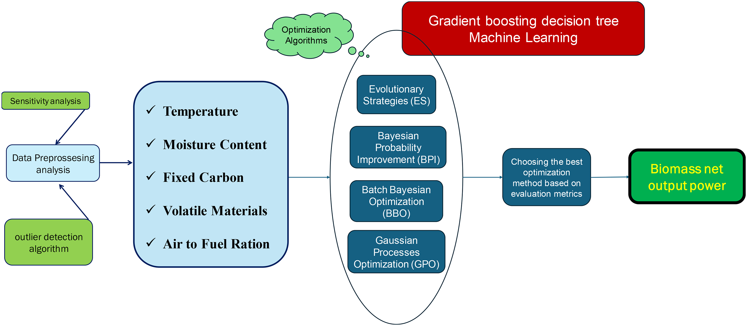
The step-by-step procedural framework adopted in this study.

GBM and optimization algorithms background

Gradient boosting machine

This study develops a predictive model utilizing the GBM framework to forecast the net output power of biomass based on proximate analysis, incorporating key input variables such as temperature, moisture content, fixed carbon, volatile matter, and air-to-fuel ratio. GBM model's hyperparameters are fine-tuned using four advanced optimization methods: BBO, ES, BPI, and GPO. The following sections describe the GBM approach and offer a brief overview of the optimization techniques applied. The GBM is a robust ML technique that combines multiple weak decision trees to form a highly accurate predictive model. Belonging to the family of boosting algorithms, GBM builds models iteratively, with each new model correcting the errors of its predecessors (Dou et al., 2025; Xiang et al., 2025). Commonly utilized for both classification and regression tasks, GBM is highly regarded for its precision and capability to model intricate, nonlinear patterns (W. Liu et al., 2022). GBM process initiates with a basic model, and in each successive iteration, a new model is incorporated into the ensemble to correct errors from prior models. These errors, known as residuals, are determined by computing the gradient of the loss function, with each new tree trained to reduce this gradient based on the ensemble's existing predictions.

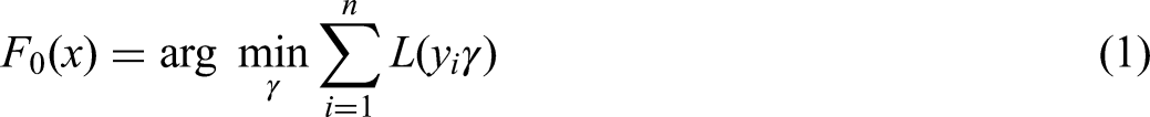
Initial model: The process starts with a rudimentary model, often a constant value, defined as follows:

F_{0} (x) = \arg min_{γ} \sum_{i = 1}^{n} L (y_{i} γ)

(1)

In this equation, L(y_i, γ) represents the loss function (e.g. MSE for regression), where γ is the initial prediction.

Residual calculation: For each iteration (m = 1, 2, …, M), residuals, or negative gradients, are computed using the below expression (Alcolea and Resano, 2021):

r_{i m} = - {[\frac{\partial L (y_{i} F (x_{i}))}{\partial F (x_{i})}]}_{F (x) = F_{m - 1} (x)}

(2)

Here, r_im denotes the residual for the i-th sample at iteration m.

Training: A new decision tree, h_m(x), is constructed to fit the residuals rim:

h_{m} (x) = \arg min_{h} \sum_{i = 1}^{n} (r_{i m} - h (x_{i}))^{2}

(3)

Ensemble update: The model is refined by incorporating the new tree, weighted by a learning rate η:

F_{m} (x) = F_{m - 1} (x) + ν h_{m} (x)

(4)

The learning rate η regulates the influence of each tree, helping to mitigate overfitting.

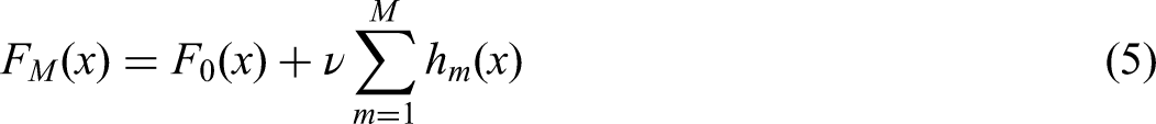
Final model: After M iterations, the complete predictive model is obtained by aggregating all trees:

F_{M} (x) = F_{0} (x) + ν \sum_{m = 1}^{M} h_{m} (x)

(5)

Optimization algorithms

Batch Bayesian optimization

BBO improves upon traditional Bayesian optimization by addressing the challenge of optimizing expensive black-box functions through the concurrent evaluation of multiple points, or batches, rather than sequential assessments. This approach capitalizes on parallel computing resources, making it particularly effective in distributed systems and high-performance computing environments where simultaneous evaluations are practical. By employing parallelism, BBO substantially reduces the total optimization time while preserving the robustness of Bayesian optimization in identifying the global optimum (González et al., 2016).

BBO evaluates several points at once instead of one by one. This demands adjustment of the acquisition function to consider how each point's evaluation may influence the others within the batch. Typically, BBO uses a Gaussian process (GP) as a surrogate model to estimate the target function, offering a probabilistic framework for predicting function behavior and quantifying uncertainty (Ren and Sweet, 2024).

BBO commonly uses acquisition functions that balance exploration and exploitation across batches. The parallel expected improvement (q-EI), an extension of EI for multiple points, estimates the expected gain over the current best value for q correlated points modeled by a GP. It is formulated as:

q - E I (x) = E [max f (x) - f (x^{+}) \cdot 0]

(6)

Here, X = [x₁, x₂, …, x_q] denotes the batch of q concurrently evaluated points, f(X) the corresponding function values, and f(x⁺) the current best observed value. The expectation E is taken over the joint posterior of the GP. Another approach in BBO is Thompson sampling, which entails sampling from the posterior distribution of the GP and selecting a batch of points that optimize the sampled function. This method effectively balances exploration and exploitation, making it well-suited for scenarios involving parallel evaluations (J. Liu et al., 2021a).

In summary, BBO enhances Bayesian optimization by leveraging parallel computing to assess multiple points simultaneously. It employs specialized acquisition functions, such as q-EI and Thompson sampling, to select batches of points that efficiently balance exploration and exploitation, ensuring robust optimization (Miyata et al., 2023). BBO excels in environments where parallel evaluations are feasible, significantly reducing optimization time while retaining the ability to locate the global optimum. Its capacity for parallel optimization positions BBO as a potent tool for tackling costly black-box functions across various applications (Tamura et al., 2025).

Bayesian probability improvement

BPI is a pivotal optimization technique within Bayesian optimization frameworks, designed to address intricate, computationally intensive functions where analytical solutions are unfeasible. This method excels in scenarios involving costly function evaluations, effectively minimizing computational overhead while proficiently locating optimal solutions (Y. Liu et al., 2021b). BPI guides optimization by balancing exploration of uncertain zones and exploitation of regions with high improvement potential.

BPI aims to raise the probability of finding points better than the current best. Unlike EI, it focuses solely on the likelihood of improvement, making it well-suited for problems where maximizing discovery chances outweighs optimizing expected gains (Jiang et al., 2018).

The theoretical foundation of BPI centers on calculating the probability that a new point x will surpass the current best value f(x*), leveraging the posterior distribution derived from GP models. These models, integral to Bayesian optimization, provide predictive mean μ(x) and variance σ²(x) across the search space. The probability of improvement is determined using the cumulative distribution function of the standard normal distribution (Y. Liu, Su et al., 2021b). The mathematical expression for BPI is given as:

BPI (x) = Φ (\frac{μ (x) - f (x^{+})}{σ (x)})

(7)

where Φ represents the cumulative distribution function of the standard normal distribution, μ(x) and σ(x) denote the predictive mean and standard deviation from the GP model at point x, and f(x⁺) signifies the best observed value of the target function so far.

The BPI acquisition function is designed to select the next points for evaluation, with higher values indicating a greater probability of exceeding the current best solution. This approach ensures consistent progress with each evaluation by prioritizing the likelihood of improvement over the scale of potential gains. As a probability-driven strategy, BPI capitalizes on the predictive uncertainties provided by GPs to steer the search for optimal solutions (Farid and Rahman, 2010). BPI focuses on improvement probability, making it a key tool in Bayesian optimization, especially when function evaluations are expensive and the aim is to maximize the chance of better results.

Evolutionary strategies

ES are optimization methods inspired by natural evolution, designed to tackle continuous optimization problems. These algorithms evolve a set of candidate solutions over generations through processes like mutation, recombination, and selection (Chen et al., 2022). Each population member is expressed as (x, σ), where x is the solution vector and σ defines the mutation step size for each variable. The process starts by initializing a population of μ individuals, with each x randomly sampled within the problem's bounds and each σ set to a small positive value, such as: x_i ∼ Uniform(x_i_min, x_i_max) and σ_i ∼ Uniform(σ_min, σ_max). In each generation, λ offspring are generated via mutation, which alters both the solution vector x and the strategy parameters σ. The new strategy parameters (σ′) are obtained as follows (Hansen et al., 2015):

\overset{'}{σ_{i}} = σ_{i} \exp (τ N (0, 1) + \overset{'}{τ} N_{i} (0, 1))

(8)

where N(0, 1) is a random variable drawn from a standard normal distribution, N_i(0, 1) is an independent random variable for each dimension, and τ and τ′ are learning rates, typically set as τ ∝ 1/√2D and τ′ ∝ 1/√(2√D). The new solution vector x′ is then determined by (Beyer and Schwefel, 2002):

\overset{'}{x_{i}} = x_{i} + \overset{'}{σ_{i}} N_{i} (0, 1)

(9)

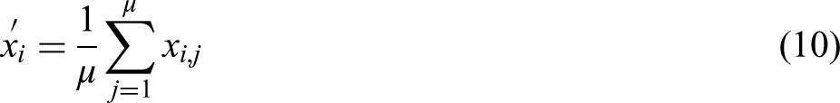
When recombination is used, it integrates information from multiple parents. For example, in intermediate recombination, the offspring (x′, σ′) is computed as the weighted average of μ parents:

\overset{'}{x_{i}} = \frac{1}{μ} \sum_{j = 1}^{μ} x_{i, j}

(10)

\overset{'}{σ_{i}} = \frac{1}{μ} \sum_{j = 1}^{μ} σ_{i, j}

(11)

After offspring are created, selection identifies the next generation. The (μ + λ)-ES scheme picks the best μ from both parents and offspring, while the (μ, λ)-ES approach selects μ only from the offspring (λ ≥ μ). ES's key strength is its self-adaptive ability to adjust the mutation parameters (σ) during optimization (Glasmachers et al., 2010). This feature enables ES to effectively balance exploration and exploitation, making it well-suited for complex, high-dimensional optimization challenges. Additionally, ES can be enhanced with advanced techniques like covariance matrix adaptation to boost its performance. In summary, ES iteratively apply mutation, recombination, and selection to refine a population of solutions. The algorithm's ability to autonomously tune its strategy parameters makes it a powerful and adaptable tool for continuous optimization. The algorithm initializes a population, generates offspring through mutation and recombination, evaluates fitness, and selects the best individuals until the stopping condition is reached. The final output corresponds to the best solution identified (X. Li et al., 2025; Mezura-Montes and Coello, 2008).

Gaussian process optimization

GPO is a powerful Bayesian optimization technique that models the target function through a GP. A GP is defined by its mean function μ(x) and covariance kernel k(x, x′), where x represents the input parameters (Majumdar et al., 2025). The covariance kernel typically adopts the squared exponential form:

k (x \overset{'}{x}) = σ_{f}^{2} \exp (\frac{{‖ x - x^{'} ‖}^{2}}{2 l^{2}}) + σ_{n}^{2} δ_{x x^{'}}

(12)

In this formula, σ_f² denotes the signal variance, l is the length scale, and σ_n² indicates the noise variance. This configuration allows GPO to provide predictions for both the mean and uncertainty across the input domain. The optimization process iteratively selects the next evaluation point by maximizing an acquisition function, such as expected improvement (EI):

EI (x) = (μ (x) - f (x^{+}) - ξ) Φ (Z) + ϕ (Z) σ (x)

(13)

Here, Φ and ϕ represent the cumulative distribution function and probability density function of the standard normal distribution, f(x⁺) signifies the best observed value to date, and ξ controls the balance between exploration and exploitation (Wang et al., 2024). This approach effectively navigates the trade-off between exploring uncertain areas and exploiting regions with high potential for improvement. GPO is particularly effective for optimizing expensive-to-evaluate functions, achieving convergence with fewer evaluations. Following each evaluation, the GP surrogate model is refined, enhancing its approximation of the target function. The posterior distribution is given by:

p (f_{*} (X y x_{*}) = N (\bar{f_{*}} cov (f_{*}))

(14)

In this expression, X encompasses all observed data points, y denotes their corresponding function values, and x* represents a new point for evaluation. This probabilistic framework facilitates efficient global optimization while offering uncertainty estimates throughout the process (Kharkovskii et al., 2020).

Methodology

Analysis of the collected database

The dataset employed to construct the ML models in this research is derived from experimental investigations into the net output power of biomass energy systems under varied conditions. Consisting of 980 data points, the dataset includes essential input variables such as temperature (°C), moisture content (%), fixed carbon (%), volatile matter (%), and air-to-fuel ratio (kg/kg), compiled from multiple sources (Safarian et al., 2020e). These parameters are critical in influencing the power output of biomass systems, making them indispensable for precise predictive modeling. The dataset captures the maximum, minimum, and average values for each variable. Of the 980 experimental samples, 90% are designated for training and validation, utilizing k-fold cross-validation with 5-fold, while the remaining 10% are set aside to evaluate the performance of the developed models.

To enhance the clarity and comprehensiveness of the dataset description, it is important to provide additional background on the biomass types included in this study. The dataset was derived from a downdraft biomass gasification–power production system modeled in Aspen Plus, incorporating 86 distinct biomass feedstocks from diverse categories. These feedstocks encompass wood and woody biomasses (e.g. pine, oak, and forest residues, accounting for approximately 35% of samples), herbaceous and agricultural biomasses (e.g. rice husk, wheat straw, sugarcane bagasse, and corn stalks, about 30%), animal-origin biomasses (e.g. poultry litter and manure, about 10%), mixed and processed biomasses (e.g. refuse-derived fuel and paper waste, about 15%), and contaminated or industrial by-product biomasses (e.g. sludge and food-processing residues, about 10%).

This diverse dataset was compiled from the thermodynamic simulation results based on the elemental and proximate analyses reported by Vassilev et al. (Adhab et al., 2025), ensuring a wide coverage of biomass compositions across different origins and processing conditions. Such diversity enables the developed ML models to capture a broad range of thermochemical behaviors, thereby improving their robustness, generalizability, and predictive reliability when applied to real-world biomass gasification systems operating under varied feedstock and process conditions.

Furthermore, Figure 2 illustrates raincloud plots for each variable, offering a comprehensive visual representation of their distributions.

Figure 2.

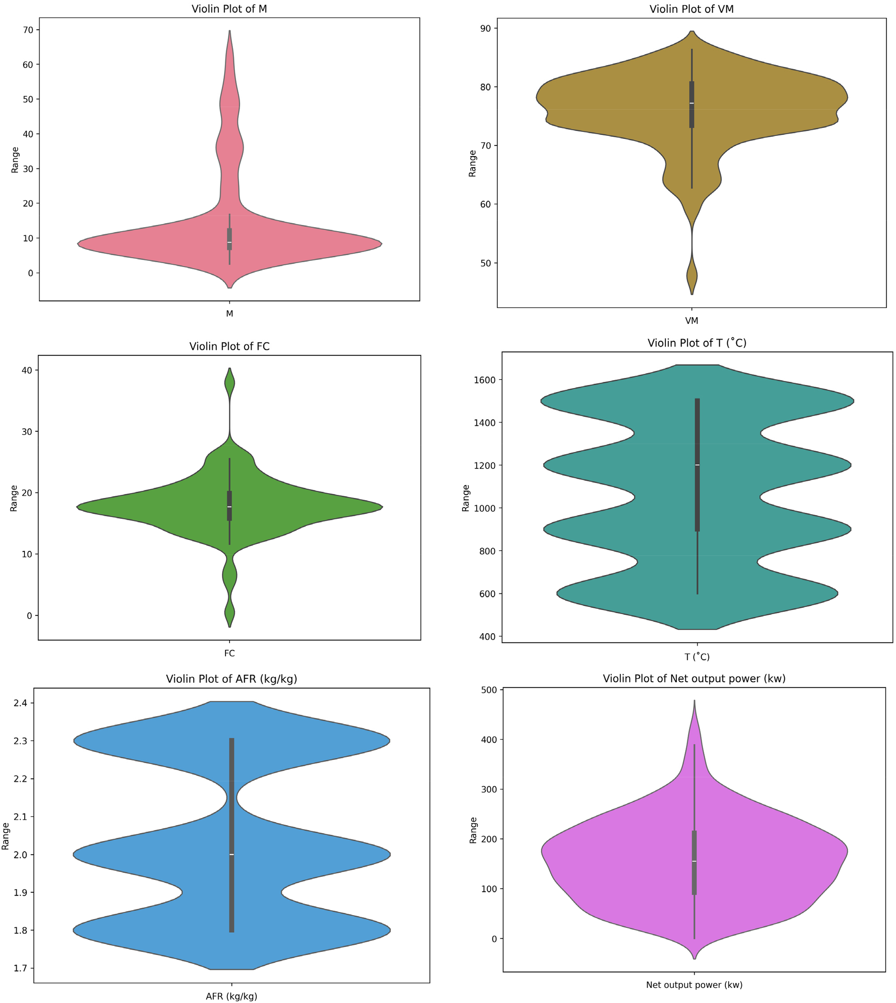
Visualization of frequency distribution and cumulative distribution for input and output data. Note that AFM means air-to-flow mass flow ratio, T is the temperature (°C), VM is the volatile materials (%), FC is the fixed carbons (%), and M is the moisture content (%).

The experimental data used for model development were generated through a thermodynamic equilibrium-based simulation of a downdraft biomass gasification integrated power production system using ASPEN Plus software. The simulated system parameters and equipment configuration were benchmarked against typical small- to medium-scale downdraft gasifiers with a thermal input capacity ranging from 25 to 250 kW. This range reflects the operational specifications of experimental and pilot-scale units reported in prior studies. For validation and data comparison, temperature measurements within the simulation framework were calibrated based on experimental findings that typically employ K-type thermocouples (chromel–alumel) with an accuracy of ±1 °C and a measurement range up to 1300 °C. The moisture content of biomass feedstocks was determined in accordance with ASTM E871-82 standard test methods for moisture analysis, while proximate and elemental analyses were performed following ASTM D3172-13 and ASTM D5373-16, respectively. These standard-based definitions and validated parameters were incorporated into the simulation to ensure the physical and chemical accuracy of the generated dataset and to maintain consistency with real-world biomass gasification operations.

Evaluation of models

The algorithm initializes a population, generates offspring through mutation and recombination, evaluates fitness, and selects the best individuals until the stopping condition is reached. The final output corresponds to the best solution identified. This approach is favored for its simplicity and ability to produce dependable, unbiased results, making it an ideal choice for various ML tasks. Its systematic structure and equitable data distribution enhance its applicability across diverse predictive modeling scenarios.

To demonstrate the k-fold cross-validation process, consider an example with 5-fold. The dataset is split into five equal parts. During the first iteration, the first fold is set aside as the validation set, with the other 4-fold used for training. In the next iteration, the second fold becomes the validation set, while the remaining folds support training. This process repeats sequentially until each fold has served as the validation set exactly once (He et al., 2025; Vujović, 2021).

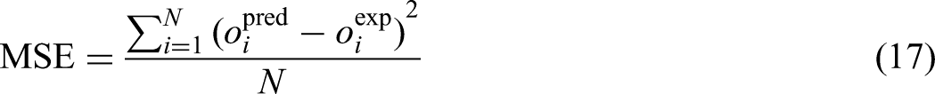
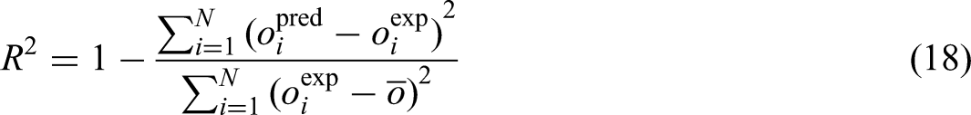
To assess the precision and reliability of the models developed in this study, a robust array of performance metrics was applied (Zhou, 2025). These include Relative Error percent or RE%, AARE%, MSE, and R². Each metric offers a unique perspective on the model's performance, as detailed in subsequent sections (Bassir and Madani, 2019; Hasanzadeh and Madani, 2024; Madani et al., 2017; Madani and Alipour, 2022):

RE % = (\frac{o^{pred} - o^{\exp}}{o^{\exp}}) \times 100

(15)

AARE % = \frac{100}{N} \sum_{i = 1}^{N} (| \frac{o_{i}^{pred} - o_{i}^{\exp}}{o_{i}^{\exp}} |)

(16)

MSE = \frac{\sum_{i = 1}^{N} {(o_{i}^{pred} - o_{i}^{\exp})}^{2}}{N}

(17)

R^{2} = 1 - \frac{\sum_{i = 1}^{N} {(o_{i}^{pred} - o_{i}^{\exp})}^{2}}{\sum_{i = 1}^{N} {(o_{i}^{\exp} - \bar{o})}^{2}}

(18)

Here, i refers to each data sample, pred and exp denote the predicted and experimental values, and N specifies the total number of samples analyzed.

The dataset for this research includes 980 data points, offering a substantial sample size for ML applications, though careful measures are still required to prevent overfitting and enhance model generalizability. To ensure balance, the distribution of the target variable (biomass net output power) was analyzed using statistical measures and visualized via density plots, revealing a broad and continuous range of output values. k-Fold cross-validation, with k = 5, was implemented to assess model performance across various data subsets, minimizing biases from training-test splits. Additionally, leverage-based outlier detection and sensitivity analysis were performed to evaluate the representativeness and impact of individual data points. Despite the advantages of a larger dataset, the use of ensemble learning through the GBM, combined with iterative cross-validation and multiple optimization techniques, ensures robustness against data variability and bolsters model stability. These integrated approaches significantly enhance the reliability of the proposed predictive framework, effectively addressing challenges related to dataset characteristics.

Results and discussion

Outlier detection

The leverage algorithm identifies data points that diverge from model expectations by combining standardized residuals with the hat matrix (H), defined as follows (Abbasi et al., 2023; Bemani et al., 2023; Madani et al., 2021):

H = X (X^{T} X)^{- 1} X^{T}

(19)

In this formula, X is an n × m matrix comprising the input variables and their respective data points, where n represents the number of samples (980) and m indicates the number of input variables (Vaja et al., 2024). The term X^T denotes the transpose of matrix X. The diagonal elements of the hat matrix H provide the hat values for each data point, measuring the influence of individual points on the predictive model. The leverage threshold (H*) is computed using the below formula (Bemani et al., 2020):

H * = 3 (n + 1) / m

(20)

Here, m and n maintain their prior definitions. For the current dataset, with n = 980 and m = 5, the leverage threshold H* is calculated as H* = 3(5 + 1)/980 ≈ 0.0184. This threshold, referred to as the leverage limit (hat value of 0.0184), serves as a critical benchmark for detecting influential data points. Data points with hat values surpassing this limit are classified as high-leverage, indicating they may disproportionately affect the model's predictions. The algorithm evaluates each point's hat value against H* to pinpoint such cases, enabling further examination of potential outliers.

This analysis is depicted through a Williams’ plot, which differentiates between trustworthy and questionable regions based on leverage values and residuals. The trustworthy region encompasses data points with low leverage (below H* = 0.0184) and small residuals, while the questionable region highlights points with either high leverage or significant residuals. Points in the questionable region warrant closer scrutiny due to their potential to compromise model accuracy. As illustrated in Figure 3, the majority of data points fall within the trustworthy region below the leverage threshold of 0.0184, labeled as Valid Data in blue. However, approximately 10 points, marked as Suspect Data in orange, exceed this threshold and are flagged as potentially problematic. This visualization tool aids in assessing data quality and the influence of anomalous points on the modeling process. Nevertheless, all points are retained in the model development to enhance the generalizability of the predictive models.

Figure 3.

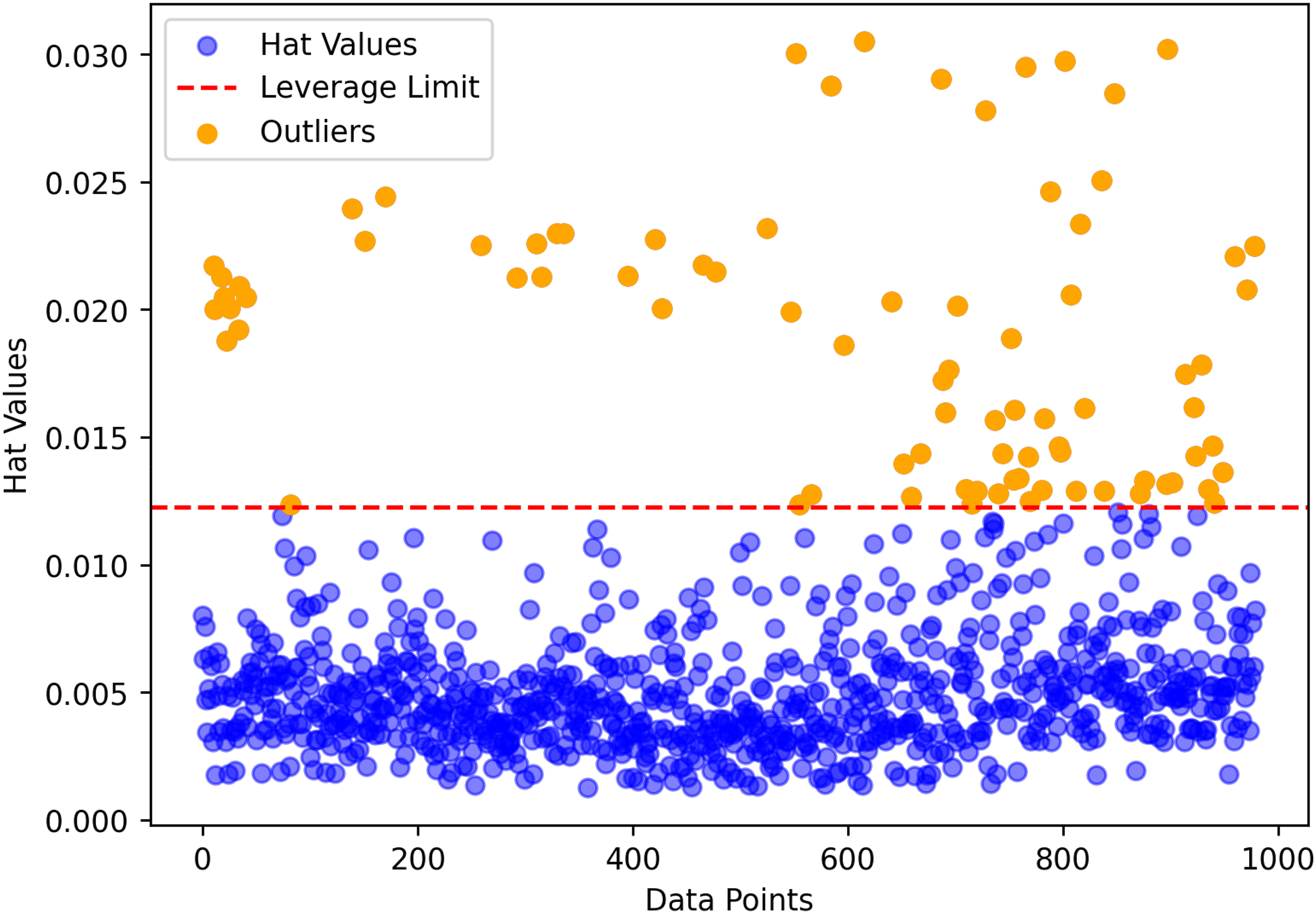
The leverage approach, a well-established technique, identifies potential outlier observations.

Sensitivity study

This section analyzes the relative impact of input variables including temperature, moisture content, fixed carbon, volatile matter, and air-to-fuel ratio on the prediction of biomass net output power based on proximate analysis. The significance of each variable is evaluated, and the correlation coefficient is calculated using the methodology described below (Bemani et al., 2023):

r_{j} = \frac{\sum_{i = 1}^{n} (x_{j, i} - {\bar{x}}_{j}) (y_{i} - \bar{y})}{\sqrt{\sum_{i = 1}^{n} {(x_{j, i} - {\bar{x}}_{j})}^{2} \sum_{i = 1}^{n} {(y_{i} - \bar{y})}^{2}}}

(21)

Here, j denotes the input variable being analyzed. The correlation coefficient (−1 to +1) reflects how strongly and in what direction the input relates to the output: values near +1 show a strong positive link, and those near −1 show a strong negative one. A positive value shows a direct link between variables, whereas a negative one signifies an inverse relation. As shown in Figure 4, the computed correlation coefficients for the input variables reveal varied relationships with biomass net output power. Among these, temperature demonstrates the strongest positive correlation (0.62), indicating that higher temperatures significantly enhance power output. Temperature is a pivotal factor in optimizing energy production, making it a crucial consideration for biomass applications. Fixed carbon exhibits a weaker positive correlation (0.14), suggesting a modest influence on power output. Moisture content shows a moderate negative correlation (−0.29), implying that higher moisture levels reduce power output to a notable extent. Volatile matter and air-to-fuel ratio have minimal negative correlations (−0.01 and −0.06, respectively), indicating negligible impacts. These findings highlight temperature as the dominant factor affecting biomass net output power, followed by moisture content and fixed carbon, with volatile matter and air-to-fuel ratio exerting minimal influence.

Figure 4.

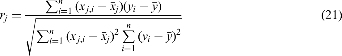
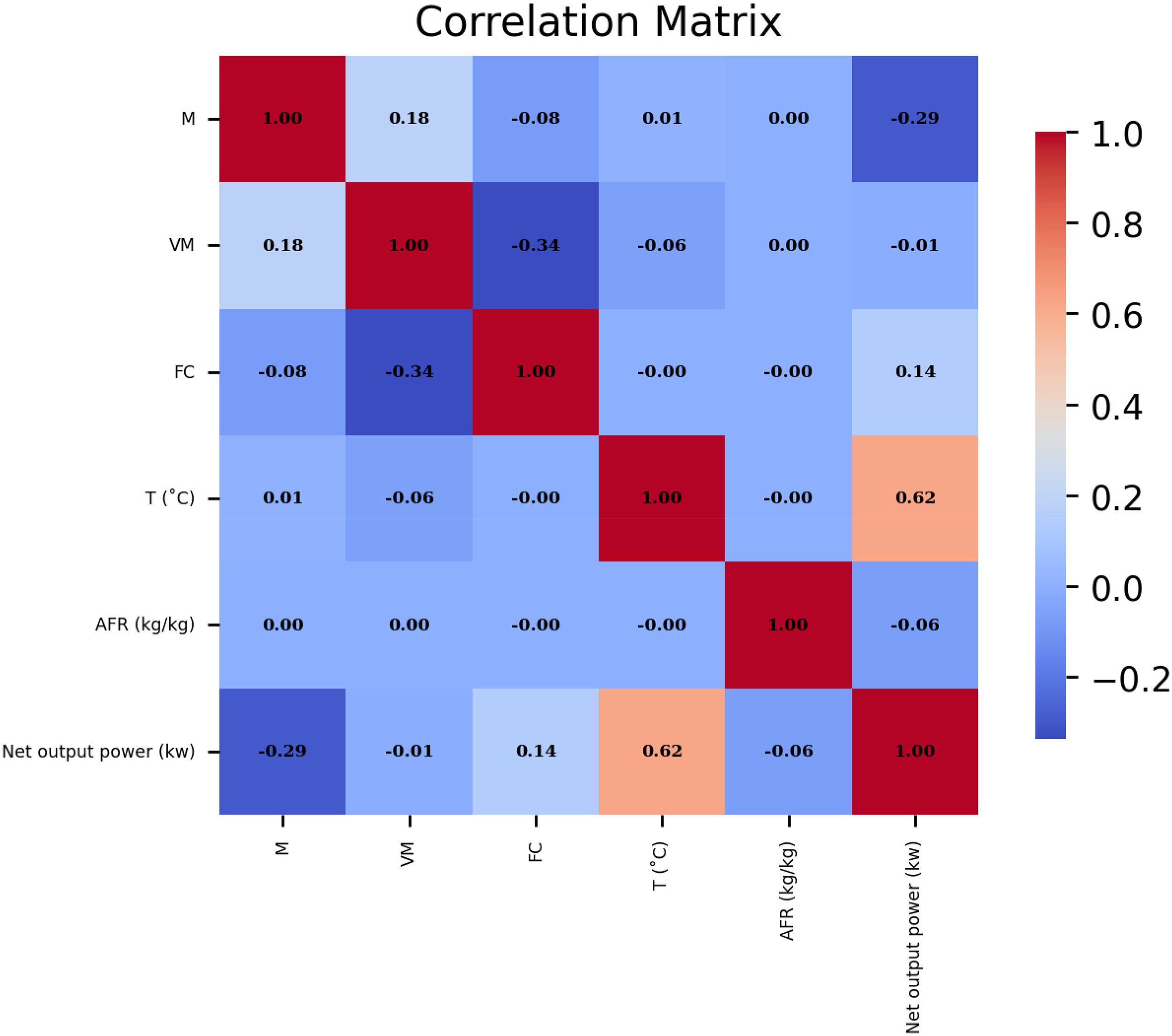
The interrelationship dynamics between paired variables as revealed through correlation analysis.

To deepen the interpretation of the correlation analysis results, the physical mechanisms underlying the observed relationships between input parameters and biomass net output power are discussed in light of thermodynamic principles. The strong positive correlation between temperature and output power (correlation coefficient: 0.62) can be attributed to the enhancement of endothermic gasification reactions at elevated temperatures. Higher temperatures accelerate the decomposition of complex biomass compounds and volatile matter, promoting the formation of combustible gases such as hydrogen (H₂), carbon monoxide (CO), and methane (CH₄). These reactions increase the energy density of the produced syngas, leading to higher net power output. Moreover, elevated temperatures facilitate tar cracking and secondary reforming reactions, further improving gas quality and combustion efficiency.

Conversely, the moderate negative correlation between moisture content and output power (correlation coefficient: −0.29) is consistent with the thermodynamic limitations imposed by high moisture levels. Excess moisture requires additional heat for evaporation during the drying and pyrolysis phases, resulting in significant energy consumption that reduces the available thermal energy for gasification reactions. This endothermic heat absorption lowers the reactor temperature and diminishes the rate of conversion of carbonaceous materials into syngas, ultimately reducing system efficiency and net power output. Therefore, the correlation findings are closely aligned with the physical and thermochemical behavior of biomass gasification, validating the model's predictive insights through both data-driven and process-based reasoning.

Models’ optimization

In this research, the hyperparameter optimization of the GBM model was performed using four advanced optimization techniques: BBO, BPI, ES, and GPO. These methods were selected to assess their effectiveness and precision in fine-tuning complex models, providing enhanced performance over traditional methods like grid search or random search due to their capability to efficiently navigate high-dimensional parameter spaces with fewer iterations. BBO and GPO utilize probabilistic surrogate models, such as GPs, to intelligently explore the hyperparameter space, while BPI emphasizes maximizing improvement probability through Bayesian acquisition functions. Conversely, ES adopts an evolutionary strategy, iteratively refining parameters during optimization. Each technique optimized five critical GBM hyperparameters: learning rate, number of estimators, minimum child weight, maximum depth, and subsample ratio. The performance of these methods is evaluated based on predictive accuracy metrics and computational efficiency, as elaborated in later sections.

These optimization algorithms were applied independently and in combination with cross-validation to fine-tune the GBM model's hyperparameters, namely the learning rate, number of estimators, minimum child weight, maximum depth, and subsample ratio. The tested ranges and the optimal values identified for each algorithm are detailed in Table 1. Additionally, Figure 5 illustrates the evolution of MSE across multiple optimization cycles, with a total of 200 iterations conducted. The hyperparameter settings resulting in the lowest MSE are documented in Table 1 (Abdelfattah et al., 2025).

Figure 5.

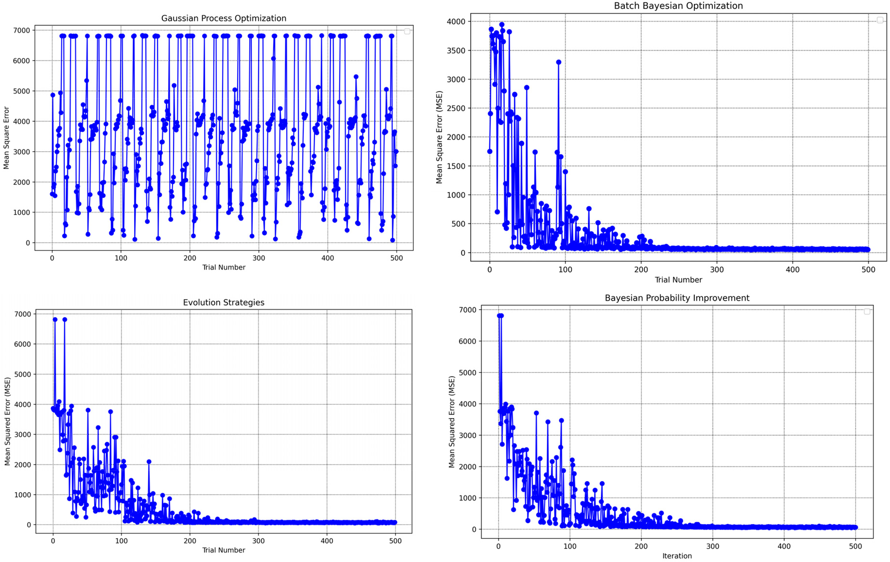
Training progression analysis: mean-squared error across iterations for various optimization approaches validated through k-fold cross-validation.

Table 1.

The random forest’s hyperparameter configurations: initial search spaces and optimized values.

Tuning parameter	Considered range	Gaussian process optimization (GPO)	Batch Bayesian optimization (BBO)	Bayesian probability improvement (BPI)	Evolution strategies (ES)
n_estimators	[50–300]	229	297	273	271
max_depth	[5–20]	13	15	13	11
max_features	[0.1–1]	0.7811200000000001	0.902533790410372	0.8177821645025559	0.9876940780718243
min_samples_split	[0.01–0.5]	0.22448979591836735	0.19276118478163176	0.2587171987260794	0.17712398218131
learning_rate	[0.01–0.3]	0.2481442524417731	0.2897394274230507	0.27492257257673836	0.27799716923669654
subsample	[0.5–1]	0.9945380063723259	0.8891173154667571	0.9983805296536963	0.8851426091109647
min_samples_leaf	[0.01–0.5]	0.030445756157134136	0.029704236969215807	0.017300956729299898	0.02788311734731056

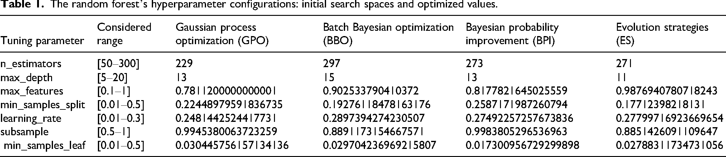
Table 2 outlines the computational time required for each optimization algorithm. BBO is the most computationally intensive, requiring 521.14 s to complete. In contrast, GPO is the most efficient, completing in 212.54 s. ES takes 437.6 s, while BPI requires 437.4 s. As indicated in Table 2, GPO achieves optimal performance relatively quickly, whereas BBO and BPI demonstrate slower but consistent improvements over iterations.

Table 2.

Assessment metrics identified for every optimization algorithm concerning training, testing, and total points.

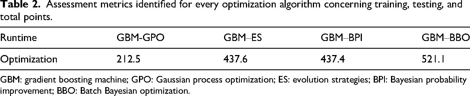
Runtime	GBM-GPO	GBM–ES	GBM–BPI	GBM–BBO
Optimization	212.5	437.6	437.4	521.1

GBM: gradient boosting machine; GPO: Gaussian process optimization; ES: evolution strategies; BPI: Bayesian probability improvement; BBO: Batch Bayesian optimization.

Table 3 provides a detailed summary of the performance metrics, including R², MSE, and AARE%, for GBM models optimized using four distinct algorithms: BBO, BPI, ES, and GPO. As shown in Figure 6, test results confirm that the BPI algorithm provides the most accurate biomass power predictions, achieving R² = 0.9947, MSE = 35.68, and AARE% = 4.5. These findings highlight BPI's capability to effectively capture the intricate relationships within the dataset while delivering robust predictive performance. In contrast, the GPO algorithm exhibits the lowest predictive accuracy, with an R² of 0.992483, a higher MSE of 50.925478, and an AARE% of 5.9032663%, making it less effective than BPI. Although BBO systematically explores the parameter space, its prolonged optimization runtime (521.14 s) diminishes its computational efficiency. Notably, the GPO algorithm demonstrates the shortest optimization time (212.54 s), underscoring its efficiency in hyperparameter tuning.

Figure 6.

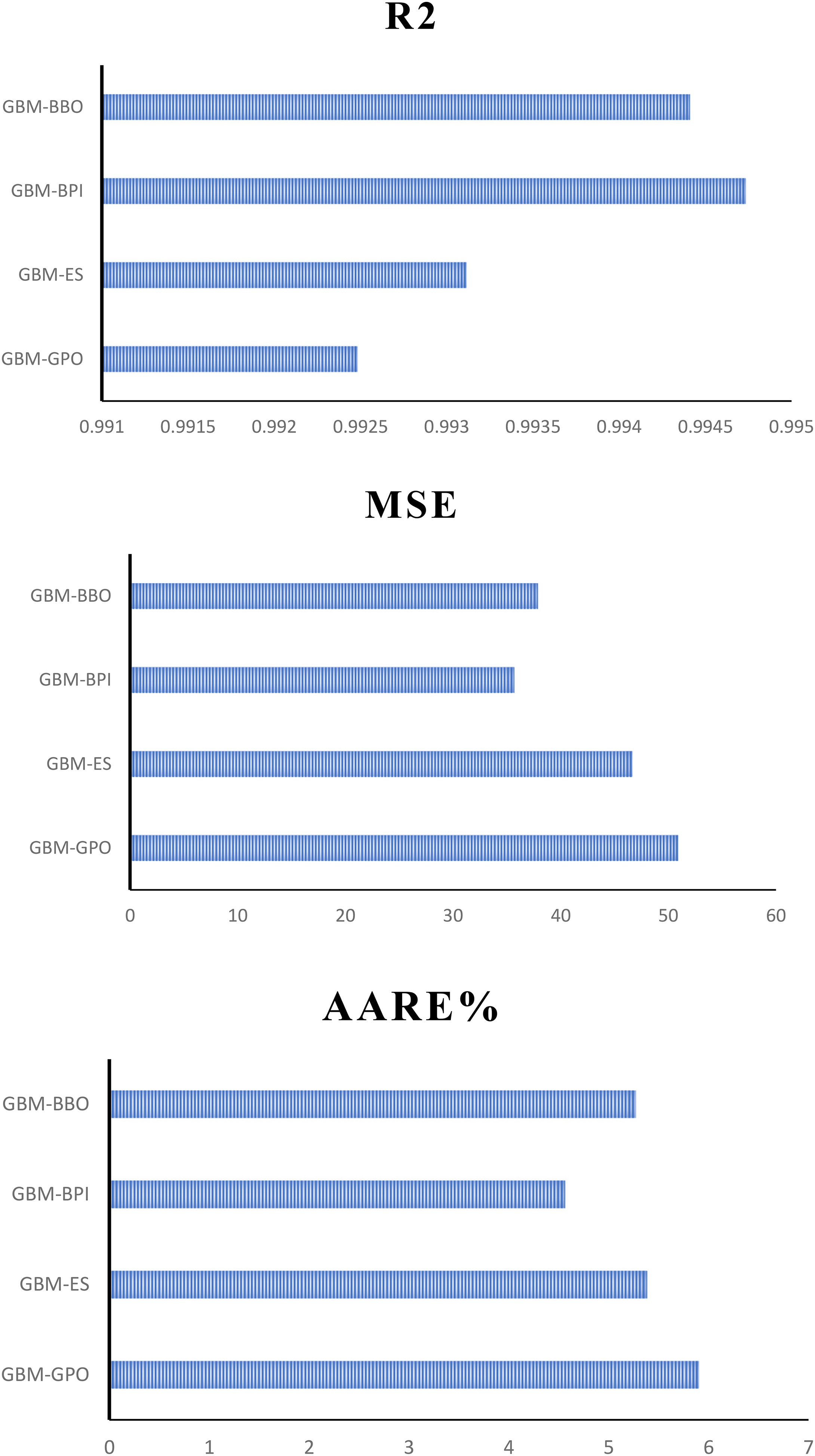
Performance assessment using R², mean-squared error, and absolute average relative error percentage during testing across all optimization approaches.

Table 3.

Assessment criteria identified for every optimization method for training, testing, and total points.

Optimization Algorithm	R ²			MSE			AARE%
Optimization Algorithm	Training	Test	Total	Training	Test	Total	Training	Test	Total
GBM–GPO	0.9972	0.9924	0.9968	18.4393	50.9254	21.6879	5.7188	5.9032	5.7372
GBM–ES	0.9983	0.9931	0.9978	12.1520	46.6467	14.3652	4.6121	5.3821	4.6891
GBM–BPI	0.9985	0.9947	0.9981	10.1536	35.6783	12.6598	4.2502	4.5601	4.2812
GBM–BBO	0.9984	0.9944	0.9980	10.6726	37.8712	13.3924	4.1272	5.2681	4.2413

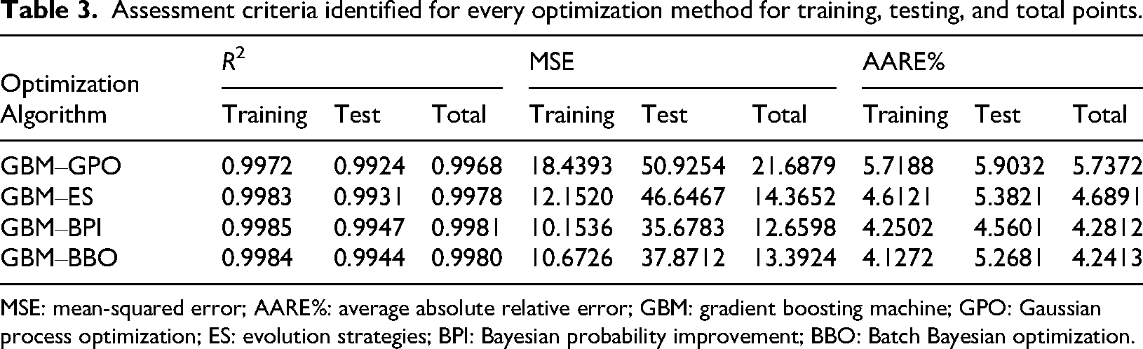
MSE: mean-squared error; AARE%: average absolute relative error; GBM: gradient boosting machine; GPO: Gaussian process optimization; ES: evolution strategies; BPI: Bayesian probability improvement; BBO: Batch Bayesian optimization.

To thoroughly assess the predictive capabilities of GBM models optimized with different techniques, Figures 7 and 8 provide visual insights into their performance. Figure 6 presents scatter plots comparing predicted versus actual biomass net output power values, for GBM models tuned with BBO, BPI, ES, and GPO. For GBM–BPI, the data points closely align with the ideal line (y = x), achieving an R² of 0.9947336 on the test set, indicating outstanding predictive precision and minimal deviations between the predicted and experimental values. Conversely, GBM–GPO (R² = 0.992483) and GBM–ES (R² = 0.9931145) show slightly more dispersed distributions, suggesting reduced accuracy, while GBM–BBO (R² = 0.9944099) displays greater scatter, underscoring its limited capacity to model the dataset's complex relationships. The regression line equations in Figure 7 for GBM–BPI closely approximate the ideal bisector (e.g. slope ≈ 1, intercept ≈ 0), affirming its excellent fit.

Figure 7.

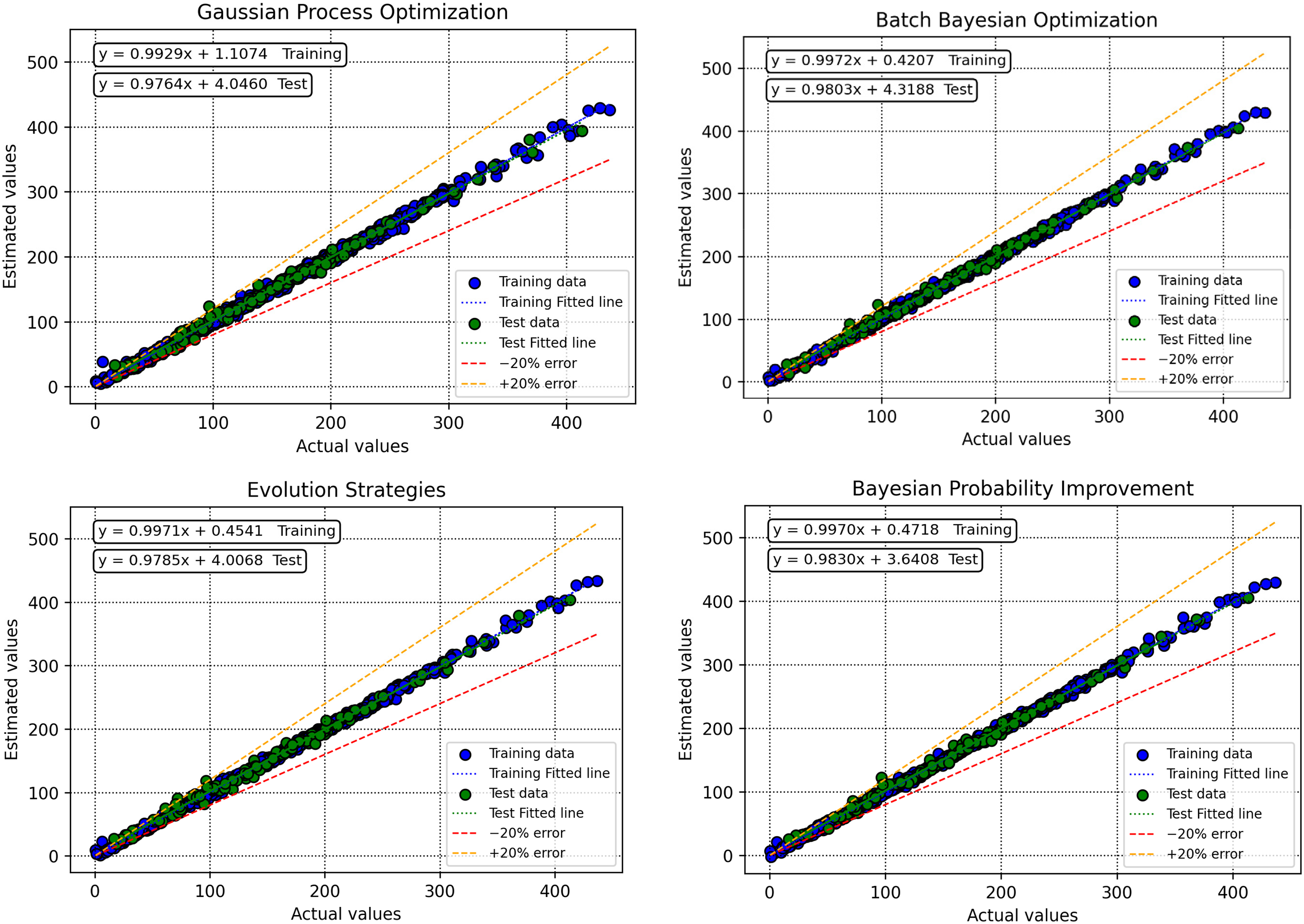
Comparison between predicted and actual values across all optimization methods during model development and evaluation.

Figure 8.

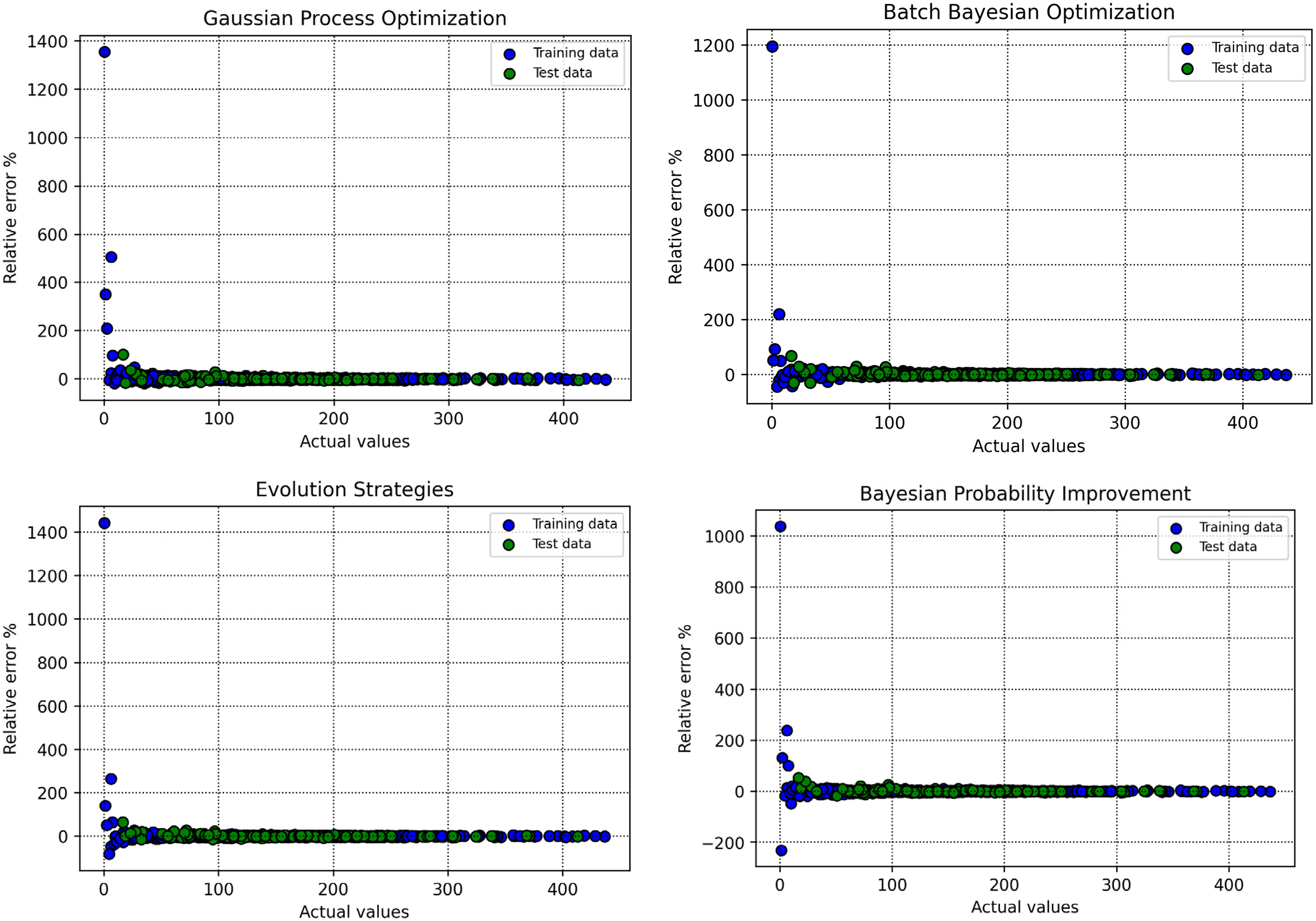
Percentage error relative to actual measurements across optimization methods during model development and validation.

Figure 8 complements this analysis by illustrating the distribution of relative errors (percentage deviations) for each optimization method. For GBM–BPI, the errors are tightly clustered around the y = 0 line, with a narrow spread and an AARE% of 4.560187% on the test set, reflecting consistent and low-error predictions. This compact error distribution underscores GBM–BPI's dependability in generating accurate biomass net output power estimates. In contrast, GBM–GPO (AARE% = 5.9032663%) and GBM–ES (AARE% = 5.3821186%) exhibit wider error ranges, while GBM–BBO (AARE% = 5.2681493%) performs less effectively. These visual trends corroborate the quantitative findings in Table 3, confirming that GBM–BPI offers the highest accuracy and reliability in predictions. This enhanced precision is particularly valuable for bioenergy applications, where accurate power output predictions can optimize system performance and minimize uncertainties in energy production. Additionally, Figure 9 compares predicted and actual data points across the four optimization algorithms.

Figure 9.

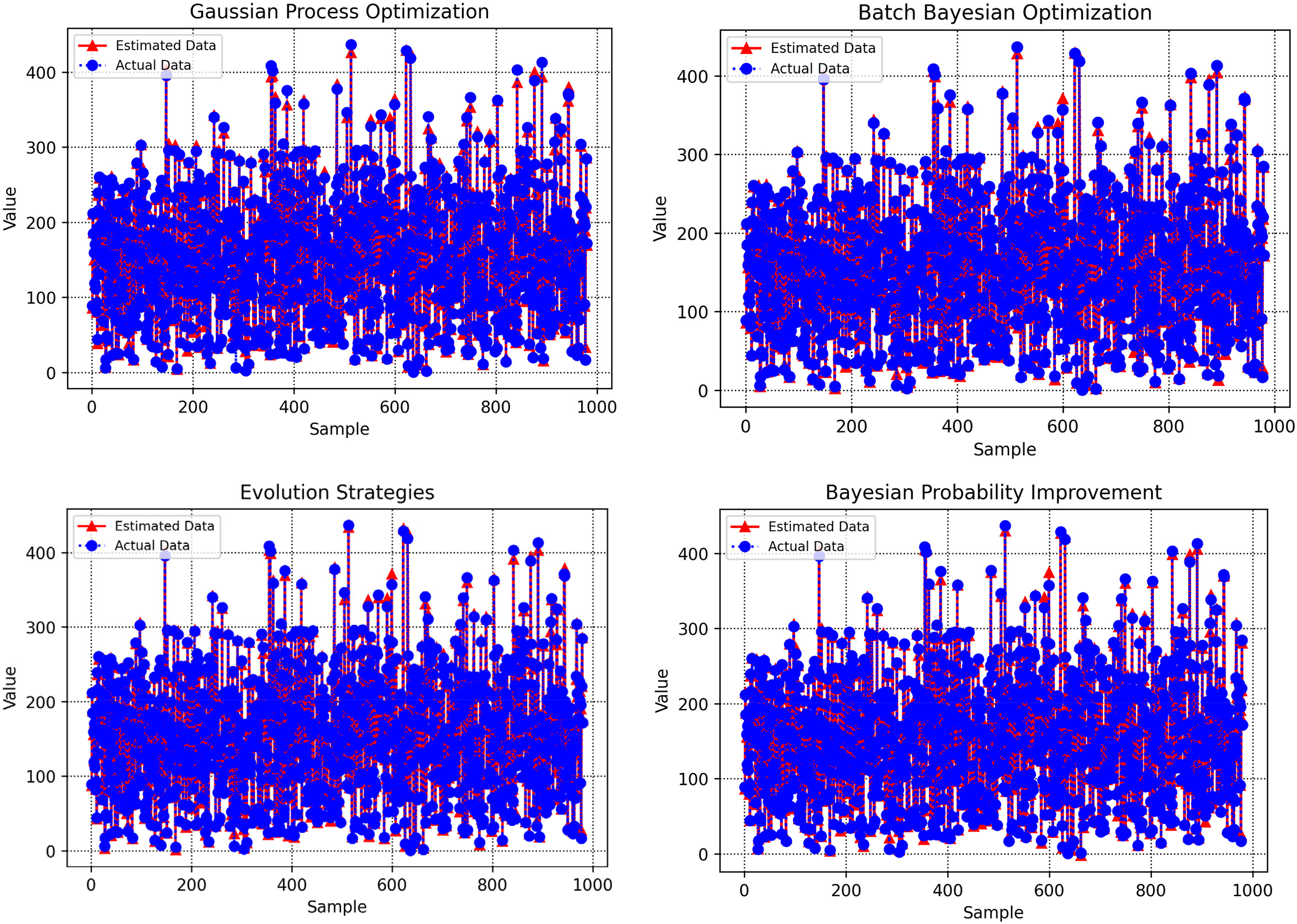
Estimated versus real data points visualization for all optimization algorithms.

Industrial applications

The predictive models established in this research, particularly the gradient boosting machine model optimized with Bayesian probability improvement (GBM–BPI), demonstrate significant potential for bioenergy applications involving biomass net output power prediction. These models provide a powerful tool for researchers and engineers to forecast power output with high precision (R² = 0.9947336 on the test set), enabling advancements across multiple domains. In bioenergy and power generation, accurate predictions of biomass net output power under varying proximate analysis conditions support the design of efficient energy production systems, capitalizing on the combustion properties of biomass to optimize performance in applications such as electricity generation, cogeneration, and biofuel production. Reliable power output predictions are essential for enhancing boiler designs and turbine efficiencies, where biomass serves as a renewable fuel source. In agricultural and waste-to-energy sectors, these models facilitate the optimization of biomass feedstock selection by predicting power output, ensuring consistent energy yields during processing. These forecasts enable precise adjustments to operational parameters, improving system reliability and energy efficiency. Moreover, in sustainable energy initiatives, such as carbon-neutral power generation and renewable energy integration, the models assist in refining process conditions by predicting power output, thereby improving energy conversion efficiency and reducing environmental impact. By minimizing reliance on expensive and labor-intensive experimental measurements, these data-driven models foster innovation, reduce operational costs, and enhance scalability. Additionally, the sensitivity analysis identifying temperature as the primary influencing factor (correlation coefficient: 0.62) provides engineers with critical insights to prioritize key variables, streamlining system optimization. Collectively, these models enable industries to leverage the energy potential of biomass, driving improved performance, sustainability, and cost-effectiveness in alignment with global demands for renewable energy solutions.

Looking forward, several opportunities exist to further enhance the predictive modeling of biomass net output power. Incorporating a broader variety of biomass compositions, temperatures, and air-to-fuel ratios would make the model more robust and improve understanding of biomass behavior in diverse settings. Investigating alternative advanced ML approaches, such as deep learning or hybrid ensemble methods beyond GBM, may better capture intricate nonlinear patterns in the data. Incorporating additional input variables, such as ash content or biomass particle size, could further refine prediction accuracy. Finally, validating these models in real-world bioenergy settings, such as biomass power plants or waste-to-energy facilities, would bridge the gap between theoretical predictions and practical applications, promoting wider adoption of data-driven strategies in energy system design and optimization.

To clarify the applicability of the proposed models in real-world settings, it is essential to specify their relevance to different types of gasification systems and discuss their computational practicality. The predictive framework developed in this study is primarily applicable to downdraft and fluidized-bed gasifiers, which are widely used in small- to medium-scale biomass power generation systems. These reactors share similar thermochemical characteristics with the data used for model training, including partial oxidation, moderate temperature ranges, and mixed feedstock compositions. Consequently, the model can reliably predict the net output power under varying operational conditions in such configurations. For large-scale or fixed-bed updraft systems, however, additional calibration or retraining with system-specific data would be necessary to prevent prediction deviations caused by differing reaction zones, gas flow dynamics, and heat transfer mechanisms.

Regarding computational efficiency, the results indicate that the GPO-based model achieved the fastest optimization time of 212.54 s, which is satisfactory for most offline design, planning, and process optimization tasks. However, for real-time or online industrial regulation, where near-instantaneous predictions are desirable, further model refinement and lightweighting are recommended. Future work may incorporate strategies such as model pruning, parameter quantization, or hybrid reduced-order modeling to minimize computational overhead while maintaining predictive accuracy. These improvements would enhance the model's suitability for embedded control systems and adaptive process management in industrial biomass gasification applications.

Industrial applications

The proposed hybrid GBM framework optimized with BPI and GPO exhibits strong potential for generalization to other complex engineering systems. In future studies, this approach can be extended to domains where predictive modeling and optimization play critical roles. Additionally, future work may focus on adapting the proposed model for process and system optimization in mechanical, industrial, and energy domains.

Conclusions

In this study, the hyperparameters of GBM model are optimized using four sophisticated optimization methods: BBO, BPI, ES, and GPO. These hybrid models are developed to forecast the net output power of biomass based on proximate analysis, utilizing a dataset of 980 experimental samples, with 90% designated for training and 10% for testing. To mitigate overfitting, k-fold cross-validation is implemented during the training process. The performance of each optimization algorithm is evaluated through critical metrics, including R², MSE, AARE%, and computational runtime. The results highlight varying degrees of influence among the input variables (temperature, moisture content, fixed carbon, volatile matter, and air-to-fuel ratio) on the target variable, net output power. Correlation analysis reveals that temperature has the most substantial effect on power output, followed by moisture content and fixed carbon, with volatile matter and air-to-fuel ratio showing minimal impact. Quantitatively, the GBM–BPI model exhibits the highest accuracy, achieving an R² of 0.9947336 on the test dataset, surpassing other optimization approaches. Its MSE is 35.678312, with an AARE% of 4.560187%. Conversely, the GBM–GPO model demonstrates the lowest performance, with a test R² of 0.992483. In terms of computational efficiency, GPO is the fastest, completing optimization in 212.54 s, compared to 521.14 s for BBO. These findings emphasize the robust potential of the proposed modeling framework for accurately and efficiently predicting biomass net output power. Future work should focus on expanding the dataset, exploring more advanced ML algorithms, and validating predictions in real-world bioenergy applications to further enhance the modeling of biomass power output.

Footnotes

ORCID iD

Abdolali Yarahmadi Kandahari

Funding

The authors disclosed receipt of the following financial support for the research, authorship, and/or publication of this article: Fujian Provincial Vocational and Technical Education Center Project (ZJGB2024049).

Declaration of conflicting interests

The authors declared no potential conflicts of interest with respect to the research, authorship, and/or publication of this article.

Data availability statement

The datasets generated in this study are available upon request from the corresponding author, subject to providing a legitimate reason for access.

References

Abbasi

Aghdam

S-y

Madani

(2023) Modeling subcritical multi-phase flow through surface chokes with new production parameters. Flow Measurement and Instrumentation 89: 102293.

Abdelfattah

Mohsin

Vora

, et al. (2025) Hybrid machine learning models for nanocomposite drilling fluid viscosity optimization. Geosystem Engineering: 1–23.

Adhab

Mahdi

Kanabar

, et al. (2025) Density of CO₂-saturated polyethylene glycol: Rigorous data evaluation and development of intelligent data-driven models. Journal of Macromolecular Science, Part B: 1–18.

Alcolea

Resano

(2021) FPGA accelerator for gradient boosting decision trees. Electronics 10(3): 314.

Baruah

Hazarika

(2017) Artificial neural network based modeling of biomass gasification in fixed bed downdraft gasifiers. Biomass and Bioenergy 98: 264–271.

Bassir

Madani

(2019) A new model for predicting asphaltene precipitation of diluted crude oil by implementing LSSVM-CSA algorithm. Petroleum Science and Technology 37(22): 2252–2259.

Begum

Rasul

Akbar

(2014) A numerical investigation of municipal solid waste gasification using ASPEN Plus. Procedia Engineering 90: 710–717.

Bemani

Baghban

Mohammadi

, et al. (2020) Estimation of adsorption capacity of CO₂, CH₄, and their binary mixtures in Quidam shale using LSSVM: Application in CO₂ enhanced shale gas recovery and CO₂ storage. Journal of Natural Gas Science and Engineering 76: 103204.

Bemani

Madani

Kazemi

(2023) Machine learning-based estimation of nano-lubricants viscosity in different operating conditions. Fuel 352: 129102.

10.

Beyer

H-G

Schwefel

H-P

(2002) Evolution strategies—A comprehensive introduction. Natural Computing 1: 3–52.

11.

Chen

, et al. (2022) Improved slime mould algorithm hybridizing chaotic maps and differential evolution strategy for global optimization. IEEE Access 10: 66811–66830.

12.

Damartzis

Michailos

Zabaniotou

(2012) Energetic assessment of a combined heat and power integrated biomass gasification–internal combustion engine system by using ASPEN Plus®. Fuel Processing Technology 95: 37–44.

13.

Dinca

Slavu

Cormoş

C-C

, et al. (2018) CO₂ capture from syngas generated by a biomass gasification power plant with chemical absorption process. Energy 149: 925–936.

14.

Dou

Zhang

, et al. (2025) Development and process simulation of a biomass driven SOFC-based electricity and ammonia production plant using green hydrogen; AI-based machine learning-assisted tri-objective optimization. International Journal of Hydrogen Energy 133: 440–457.

15.

Farid

Rahman

(2010) Anomaly network intrusion detection based on improved self adaptive Bayesian algorithm. Journal of Computers 5(1): 23–31.

16.

George

Arun

Muraleedharan

(2018) Assessment of producer gas composition in air gasification of biomass using artificial neural network model. International Journal of Hydrogen Energy 43(20): 9558–9568.

17.

Glasmachers

Schaul

, et al. (2010) Exponential natural evolution strategies. In: Proceedings of the 12th annual conference on Genetic and evolutionary computation, pp. 393–400.

18.

González

Dai

Hennig

, et al. (2016) Batch Bayesian optimization via local penalization.

19.

Hansen

Arnold

Auger

(2015) Evolution strategies. In: Kacprzyk J and Pedrycz W (eds) Springer Handbook of Computational Intelligence. Berlin, Heidelberg: Springer, 871–898.

20.

Hasanzadeh

Madani

(2024) Deterministic tools to predict gas assisted gravity drainage recovery factor. Energy Geoscience 5(3): 100267.

21.

Zio

Yang

, et al. (2025) A systematic resilience assessment framework for multi-state systems based on physics-informed neural network. Reliability Engineering & System Safety 257: 110866.

22.

Jiang

Liang

Gao

, et al. (2018) An improved constraint-based Bayesian network learning method using Gaussian kernel probability density estimator. Expert Systems with Applications 113: 544–554.

23.

Kharkovskii

Ling

Low

BKH

(2020) Nonmyopic Gaussian process optimization with macro-actions.

24.

Liu

Wang

, et al. (2025) Catalytic cracking of biomass tar for hydrogen-rich gas production: Parameter optimization using response surface methodology combined with deterministic finite automaton. Renewable Energy 241: 122368.

25.

Liu

Jiang

Zheng

(2021a) Batch Bayesian optimization via adaptive local search. Applied Intelligence 51(3): 1280–1295.

26.

Liu

Fan

Xia

(2022) Credit scoring based on tree-enhanced gradient boosting decision trees. Expert Systems with Applications 189: 116034.

27.

Liu

, et al. (2021b) Improved naive Bayesian probability classifier in predictions of nuclear mass. Physical Review C 104(1): 014315.

28.

Madani

Abbasi

Baghban

, et al. (2017) Modeling of CO₂-brine interfacial tension: Application to enhanced oil recovery. Petroleum Science and Technology 35(23): 2179–2186.

29.

Madani

Alipour

(2022) Gas-oil gravity drainage mechanism in fractured oil reservoirs: Surrogate model development and sensitivity analysis. Computational Geosciences 26(5): 1323–1343.

30.

Madani

Moraveji

Sharifi

(2021) Modeling apparent viscosity of waxy crude oils doped with polymeric wax inhibitors. Journal of Petroleum Science and Engineering 196: 108076.

31.

Majumdar

Mojahed

Nazari

(2025) Inverted Gaussian process optimization for nonparametric Koopman operator discovery. arXiv preprint arXiv:2504.00304.

32.

Mezura-Montes

Coello

CAC

(2008) An empirical study about the usefulness of evolution strategies to solve constrained optimization problems. International Journal of General Systems 37(4): 443–473.

33.

Mikulandrić

Lončar

Böhning

, et al. (2014) Artificial neural network modelling approach for a biomass gasification process in fixed bed gasifiers. Energy Conversion and Management 87: 1210–1223.

34.

Miyata

Kasahara

Yamada

, et al. (2023) Exploring autonomous optimal experimental conditions for in vitro tissue maturation with batch Bayesian optimization.

35.

Pettinau

Ferrara

Amorino

(2013) Combustion vs. gasification for a demonstration CCS (carbon capture and storage) project in Italy: A techno-economic analysis. Energy 50: 160–169.

36.

Puig-Arnavat

Hernández

Bruno

, et al. (2013) Artificial neural network models for biomass gasification in fluidized bed gasifiers. Biomass and Bioenergy 49: 279–289.

37.

Ren

Sweet

(2024) Optimal initialization of batch Bayesian optimization. arXiv preprint arXiv:2404.17997.

38.

Safarian

Richter

Unnthorsson

(2019a) Waste biomass gasification simulation using ASPEN Plus: Performance evaluation of wood chips, sawdust and mixed paper wastes.

39.

Safarian

Saryazdi

SME

Unnthorsson

, et al. (2020e) Dataset of biomass characteristics and net output power from downdraft biomass gasifier integrated power production unit. Data in Brief 33: 106390.

40.

Safarian

Sattari

Hamidzadeh

(2018) Sustainability assessment of biodiesel supply chain from various biomasses and conversion technologies. Biophysical Economics and Resource Quality 3: 1–15.

41.

Safarian

Unnþórsson

Richter

(2019b) A review of biomass gasification modelling. Renewable and Sustainable Energy Reviews 110: 378–391.

42.

Safarian

Unnthorsson

(2018) An assessment of the sustainability of lignocellulosic bioethanol production from wastes in Iceland. Energies 11(6): 1493.

43.

Safarian

Unnthorsson

Richter

(2020a) Performance analysis and environmental assessment of small-scale waste biomass gasification integrated CHP in Iceland. Energy 197: 117268.

44.

Safarian

Unnthorsson

Richter

(2020b) Simulation and performance analysis of integrated gasification–syngas fermentation plant for lignocellulosic ethanol production. Fermentation 6(3): 68.

45.

Safarian

Unnthorsson

Richter

(2020c) Simulation of small-scale waste biomass gasification integrated power production: A comparative performance analysis for timber and wood waste.

46.

Safarian

Unnthorsson

Richter

(2020d) Techno-economic and environmental assessment of power supply chain by using waste biomass gasification in Iceland. Biophysical Economics and Sustainability 5: 1–13.

47.

Safarianbana

Unnthorsson

Richter

(2019) Development of a new stoichiometric equilibrium-based model for wood chips and mixed paper wastes gasification by ASPEN Plus.

48.

Tamura

Job

Chang

, et al. (2025) Autonomous organic synthesis for redox flow batteries via flexible batch Bayesian optimization.

49.

Vaja

Rana

Thakor

, et al. (2024) AC/Dc conductivity and ML-based evaluation of electric characteristics of methylene blue solution. Journal of Molecular Liquids 410: 125676.

50.

Vujović

(2021) Classification model evaluation metrics. International Journal of Advanced Computer Science and Applications 12(6): 599–606.

51.

Wang

Zhang

, et al. (2024) Continuous Gaussian process pre-optimization for asynchronous event-inertial odometry. arXiv preprint arXiv:2412.08909.

52.

Xiang

Wang

, et al. (2025) Enhancing beef tallow flavor through enzymatic hydrolysis: Unveiling key aroma precursors and volatile compounds using machine learning. Food Chemistry 477: 143559.

53.

Zhou

(2025) GWO-GA-XGBoost-based model for radio-frequency power amplifier under different temperatures. Expert Systems with Applications 278: 127439.

Hybrid gradient boosting machine for precise prediction of biomass net output power in terms of proximate analysis

Abstract

Keywords

Introduction

GBM and optimization algorithms background

Gradient boosting machine

Optimization algorithms

Batch Bayesian optimization

Bayesian probability improvement

Evolutionary strategies

Gaussian process optimization

Methodology

Analysis of the collected database

Evaluation of models

Results and discussion

Outlier detection

Sensitivity study

Models’ optimization

Industrial applications

Industrial applications

Conclusions

Footnotes

ORCID iD

Funding

Declaration of conflicting interests

Data availability statement

References