
Abstract
Among various fuel cells (FCs), Polymer exchange membrane FC (PEMFC) plays a vital role in the transportation era because they operate at moderate temperatures, have quick start-up, are highly efficient, have scalable size, have high energy density etc. With a high degree of accuracy, machine learning algorithms (MLAs) can be applied to solve nonlinear problems in FCs, including performance prediction, service life prediction, and fault diagnostics. In addition to carrying out the optimization of operational parameters and design, MLAs when paired with optimization techniques may effectively and accurately accomplish a variety of optimization goals. The main objective of this study is to explain the significance of MLAs in PEMFC research and describe the prediction of operating parameters at which the PEMFC performance is maximized. This paper is structured to study the influence of different process parameters such as system temperature, fuel supply pressure, air supply pressure, fuel flow rate and air flow rate on the output voltage of the FC. It is clearly observed that the system temperature has significant percentage contribution as 96.92% on FC current and 86.22% on FC voltage compared to other parameters. Different MLAs are modelled to explore the PEMFC performance and results proved that gradient boosting regression provides better predictions compared to other algorithms such as decision tree regressor, support vector machine regressor, and random forest regression.
Introduction
Fossil fuel has become the worst concern among people all over the globe since it is on the verge of extinction. It is expected to last for the next 30 years as per International Energy Agency Statistics (IEA) statics 2016. Because of its ill effects, people have started to use non-conventional energy resources in their day-to-day activities (Awad et al., 2024), (Awad et al., 2023), (Atia et al., 2024). Among the non-conventional resources, hydrogen energy possesses the most significant features such as low operating temperature, moderate efficiency, quick start up and scalable size and affordable to the end user. The fuel cell is a fascinating hydrogen technology as it does not pollute the environment, is silent in operation, has moderate operating temperature and quick start-up. Based on the electrolyte used in the fuel cell (FC), there are five types of FC, namely: alkaline, molten carbonate, phosphoric acid, polymer electrolyte membrane (PEM), solid oxide, direct methanol. PEM plays a vital role in the transportation era because it is operating at moderate temperatures, have quick start-up, is highly efficient, is scalable in size, have high energy density etc. The following describes the prediction of operating parameters at which the PEM performance is maximized (Ashfaq et al., 2024), (Joga et al., 2024), (Krishnan et al., 2024), (Kassem et al., 2024).
Various machine learning algorithms have been used to model the PEM operation and its attributes (Almodfer et al., 2022), (Ashraf et al., 2022), (Legala, Zhao and Li, 2022), (Metwally Mahmoud, 2023), (Yue et al., 2022). In their study, they found that the support vector model (SVM) was effective when the output of the FC was one variable and the artificial neural network (ANN) model was found accurate when there was multiple output variable regression. The evaluation methods for PEM performance, life span and fault detection using a machine learning model have been proposed (Su et al., 2023), (Deng et al., 2022), (Elmetwaly et al., 2023), (Paciocco, Cawte and Bazylak, 2023). They used common machine learning algorithms (MLAs) such as ANN, SVM and random forest model (RFM) for evaluation. They reported that the proper selection of machine models was essential for the evaluation of PEM attributes.
The dynamic humidity was considered to analyze the performance of the PEM by (Saco et al., 2022), (Ibrahim et al., 2023). There were three MLAs used to maximize the performance such as SVM, linear regression model (LRM) and K-nearest neighbor model (KNNM). The LRM yielded better results than other methods and reported to use deep learning network model in future to analyze the performance. The parameters estimation using honey badger optimization (HBO) for accurate modelling and optimizing the performance of PEM by (Almodfer et al., 2022), (Wang et al., 2024), (Zhang et al., 2024). The data set was obtained by conducting an experimental series on 250-W stack, 500-W stack and Nedstack PS6 which were analyzed using the proposed HBO algorithm. The results outperformed the other algorithms used in the literature.
A survey was conducted by (Ashraf et al., 2022) to study the parameter estimation methods proposed by various researchers in the engineering era to enhance the performance of PEM. Various meta-heuristic algorithms used over the decade were studied in this survey. There were 34 Meta-heuristic algorithms compared comprehensively to make a clear picture of algorithm performance to the readers. A single-solid oxide chamber fuel cell was modelled using ANN and GA by (Le, Nguyen and Nguyen, 2019). It was reported that the ANN-based model could describe the SOFC attributes effectively without having knowledge of the electrochemical model of the system. The power density was considered to be a fitness function and maximized the performance when the operating temperature and fabrication temperature were kept at the prescribed value.
A novel parameter estimation of PEM has been proposed by (Fathy, Abdel Aleem and Rezk, 2021). The proposed technique called the Lshade- Epsin optimization method was applied to commercial PEM and compared the results against former optimization methods to prove the effectiveness of the proposed scheme. MLAs and ANN had the potential to make the PEM feasible for transportation and static power generation applications. (Wang et al., 2020) reviewed the effectiveness of ANN and MLA in the optimization of PEM geometry, prediction of dynamic operating parameters and selection of materials used for catalyst based on past data. The fault diagnosis methods for PEM using electrochemical spectroscopy impedance and deep learning networks were proposed by (Lv et al., 2024). The proposed framework had good computational efficiency and greater feasibility in diagnosing the fault in PEM cells.
The operating parameter maintenance of the PEM was the crucial task and identification of the most dominating parameter of the PEM became difficult as reported by (Dhanya and Hareendran, 2021). A 25 V/20A PEM was tested with different ML models and concluded that the Tertius model was found better for the prediction of dynamic operating parameters. The pressure and flow rates of fuel and air were the most significant parameters and helpful in finding the voltage and power of PEM as reported by (Wilberforce and Biswas, 2022). Their study revealed that the optimized parameters could yield better performance using ANN. The operating parameters and design specifications must be optimized for better performance of the PEM reported by (Karthikeyan et al., 2013). The optimization was carried out using Multiphysics COSMOL software 4.2 packages. The Tuguchi method yielded the result that fuel pressure had a great impact on the performance of the PEM cell.
The voltage degradation and life span of PEM have become major concerns when it is adopted for transportation applications. The MLAs were constructed to forecast the voltage degradation and durability of the FCs (Liu et al., 2022). The combination of the SVM with a long short-term memory model yielded better forecasting capability than other methods. The gas distribution quality parameter had a greater impact on the performance of the PEM when it was used in a high-temperature range as stated by (Deng et al., 2022). A data-driven surrogate model was developed to forecast the gas distribution parameter. This study revealed the guidelines to forecast the durability of FCs for high-temperature usage.
Background of PEM
A PEM-FC is an electrochemical device which produces electricity through chemical reactions. The hot water is produced as a by-product which can be utilized for some other purposes. The hydrogen fuel is supplied at the anode in which the hydrogen ion and electron are separated. The electrons liberated from the anode reach the cathode through an external resistance which constitutes an electric current whereas the hydrogen ion transfers through a porous polymer electrolyte to reach the cathode. The oxygen is supplied at the cathode where the hydrogen ion reacts with oxygen and electrons to form hot water as a by-product (Ahmad et al., 2022), (Unnikrishnan, Rajalakshmi and Janardhanan, 2018).
Mechanistic model of PEM
It is an accurate model since it estimates flow of input and changes in energy inside PEM are being taken into account. This mathematical model is derived based on some assumptions like conservation of energy, electrochemical reactions and heat transfer. The simulation of electrochemical mathematical equations provides the performance of electrodes and electrolytes thereby the output performance indicators can be revealed. The thermodynamics simulation provides information regarding energy conversion efficiency under different temperature and thermal management design can be carried out easily. The fluid mechanics simulation yields information regarding pressure drops due to distribution of hydrogen and oxygen in its channel and useful in designing water management system. Though it possesses lot of advantages, but it is difficult to use in experimental analysis because of involvement of more parameters and its analysis (Ahmad et al., 2022), (Dudek et al., 2020).
Mathematical modelling is quite important to know the operating parameters which determine the behavior of FCs. The thermodynamics modelling does not give information about the rate at which electricity is produced due to chemical reactions and hence electrochemistry modelling is preferred in this research. The loss that occurred during the chemical reaction can easily be predicted by this modelling. The following section elucidates the electrochemistry modelling of PEM cells (Ghasemi et al., 2022), (Atyabi et al., 2019).
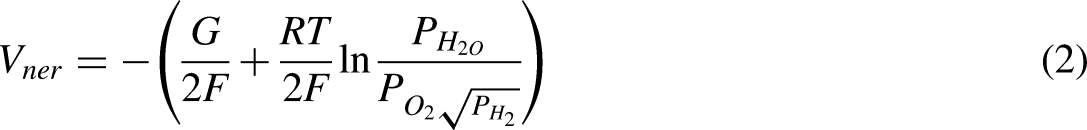
The output voltage of the PEM can be written as:

Activation loss
Due to slowness of chemical reaction taking places at both anode and cathode initially, the voltage drop is resulted. It occurs at both the electrodes, though the impact is more on cathode electrode because the reduction reaction takes more potential than oxidation reaction. The activation loss can be minimized by any of the methods addressed below (Arshad et al., 2019).
use the most effective and appropriate catalytic material making irregular surface of electrodes Increasing the concentration of oxygen in air Increasing the operating pressure
α is the coefficient of charge transfer, id is the current density, and ir is the current density corresponds to reaction exchange, and iL is the limiting current density.

Mass transport loss
This loss is mainly due to concentration of fuel and air used as the concentration of reactants has major impact on output voltage. Since the reduction of concentration of reactants would result in slow down or stopping the reactants transport to the surface of electrodes, it is often called as mass transport loss (Xu et al., 2024).

Ohmic loss
The resistance offered by electrolyte membrane and electrode causes voltage drop called ohmic loss. The electrolyte offers a resistance to the protons and electrode offers a resistance to the flow of electrons. The total resistance can be minimized by using any of the following methods (Xu et al., 2024).
Using the high conductivity electrode material proper designing of contact surface and electrodes By reducing the thickness of electrolyte used.
R(ano + cat) is the resistance of anode and cathode. From the electrochemistry modelling of the PEM, it is obvious that the operating parameters like fuel supply pressure, fuel flow rate, temperature, air supply pressure, and airflow rate decide the output voltage of the PEM at any cost.

Experimentation
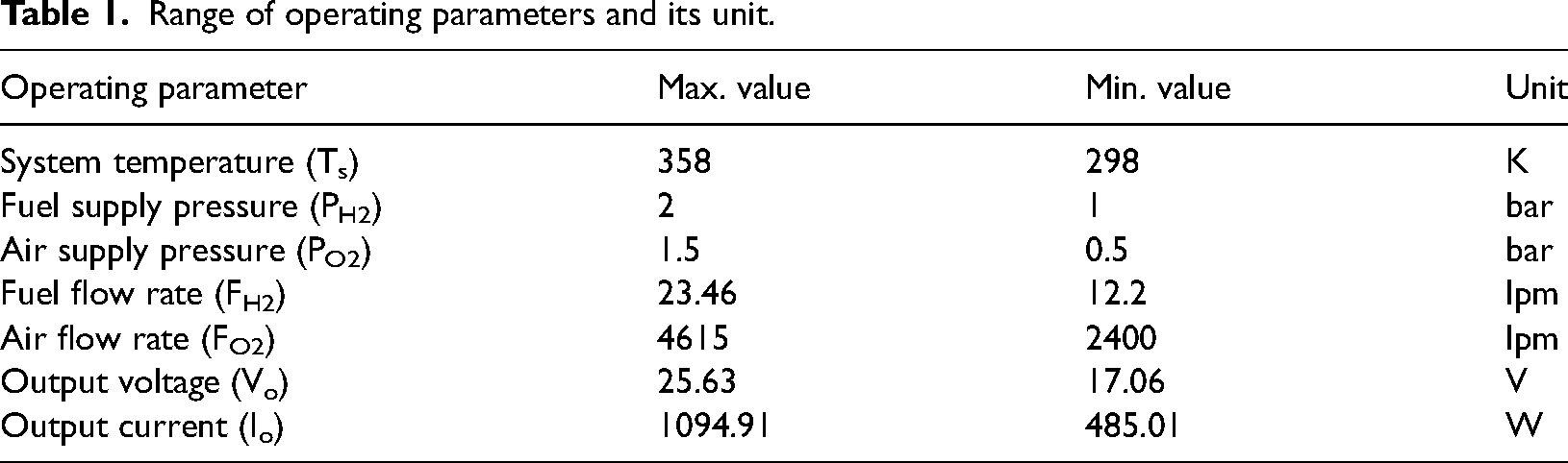
From the mathematical modelling of PEM, there are a number of factors that influence the output voltage and output power of PEM as seen in Figure 1. To predict the optimized operating conditions, it is essential to carry out experimentation on PEM. A 1.26 kW PEM with an open circuit voltage of 24 V is considered for this study in which 42 cells are connected in the stack. The hydrogen fuel, oxygen and water are supplied with a ratio of 98.3:27.3:1. The expected nominal efficiency of the stack is 46% and the nominal voltage and current of the proposed PEM are 52 A and 24.3 V, respectively. The polarization characteristics of PEM are depicted in Figure 2 and Figure 3. The operating parameters such as system temperature, fuel supply pressure, air-supply pressure, fuel flow rate and air-flow rate are varied from minimum value to maximum value as listed in Table 1. To find the most significant factor using statistical analysis, it is required to conduct level number of operating parameters experiments to be carried out. Here there are 3 levels and 5 parameters are considered and hence total of 243 experiments carried out. A statistical analysis has been carried out to find the percentage significance of operating parameters in deciding the output voltage and output power of PEM. It is inferred that the system temperature (51.3%) is the most significant factor and air-flow rate (0.02%) is the least significant factor as shown in Figure 4. The interaction of the most significant factor i.e., system temperature Vs least significant factor i.e., air flow rate Vs output parameters i.e., output voltage and output power are depicted in Figure 5. Recognizing that system temperature is the most significant parameter influencing PEM performance has wide-ranging implications for both the design and operation of these cells. Effective thermal management is crucial, impacting everything from material selection and stack design to operational strategies and system integration. By optimizing temperature control, designers and operators can significantly enhance the efficiency, reliability, and durability of PEM, making them more viable for a variety of applications.
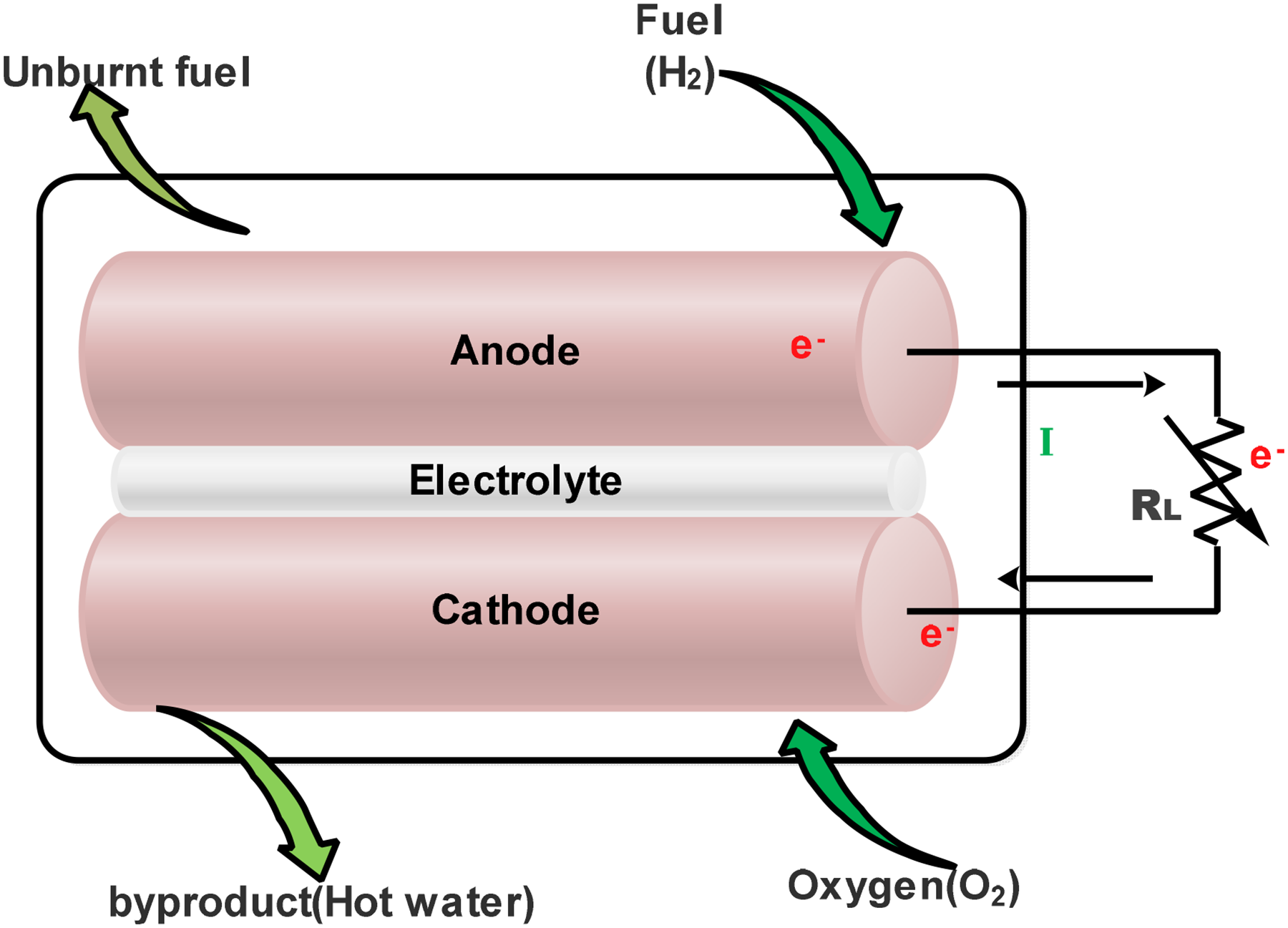
The construction of PEMFC.
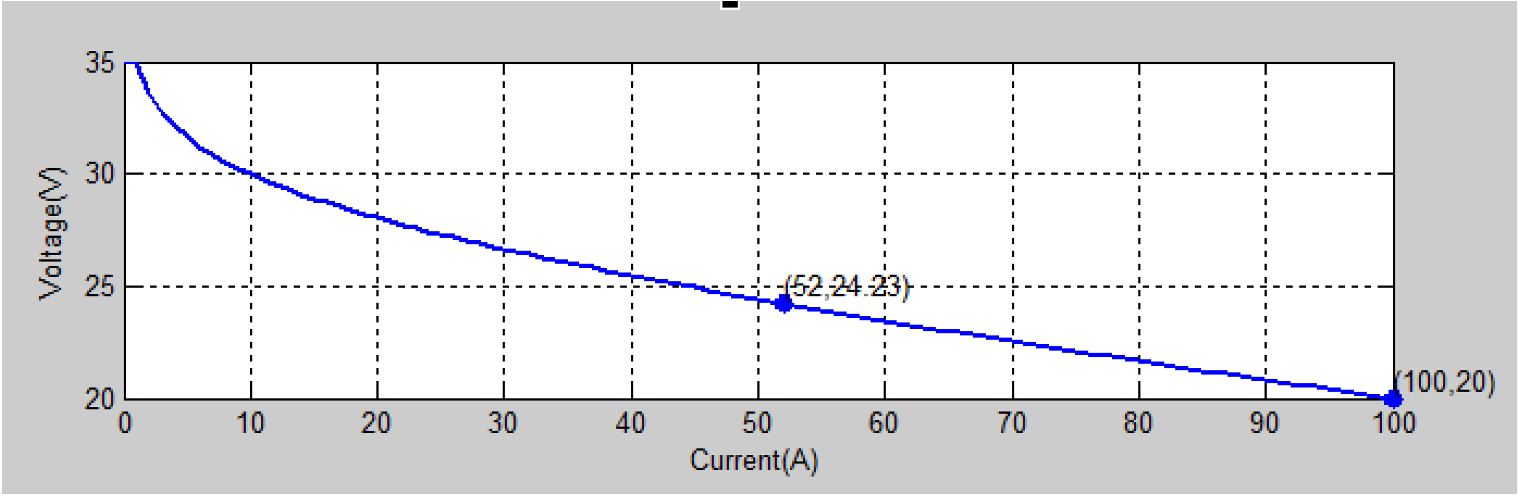
Voltage Vs current characteristics of 1.26 kW PEM.
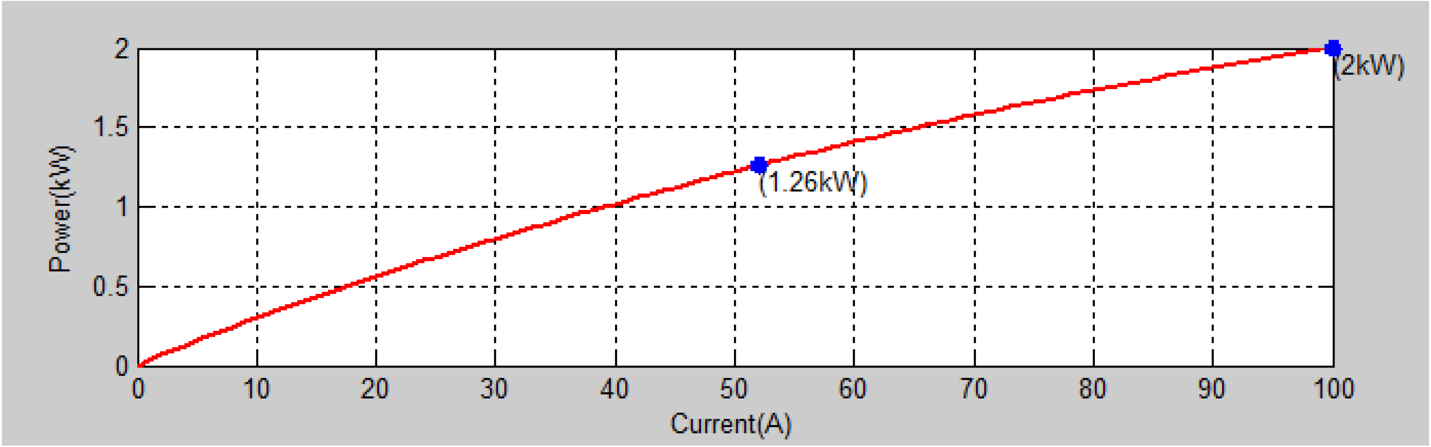
Power Vs current characteristics of 1.26 kW PEM.
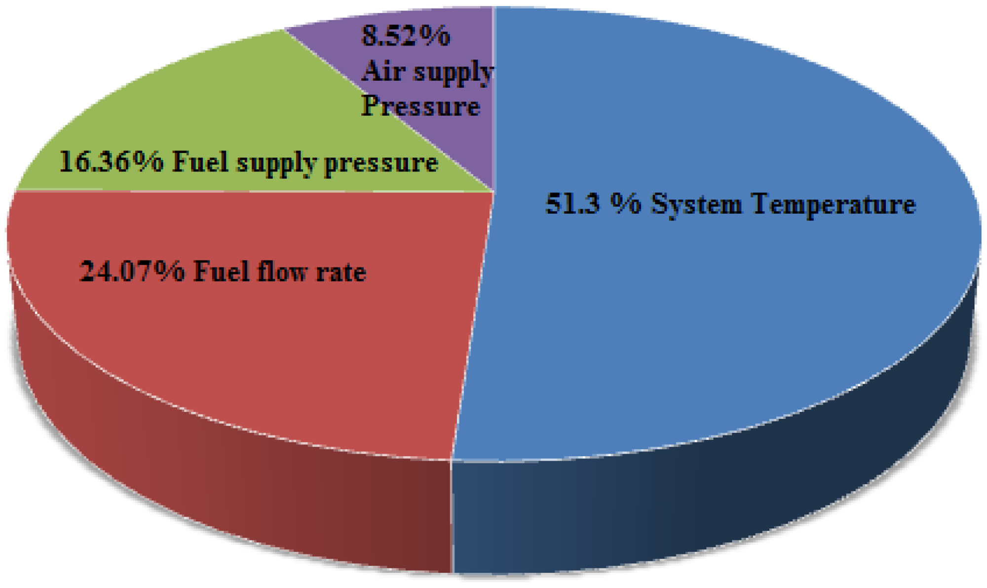
The percentage significance of operating parameters. (a) Output voltage Vs system temperature, and Vs air-flow rate. (b) Output power Vs system temperature Vs air-flow rate.
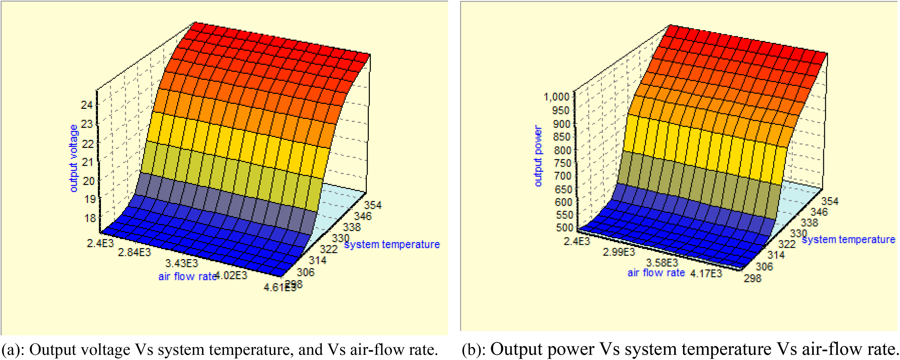
Output voltage and power Vs system temperature, and Vs air-flow rate.
Range of operating parameters and its unit.
Regression analysis: FC current (A)
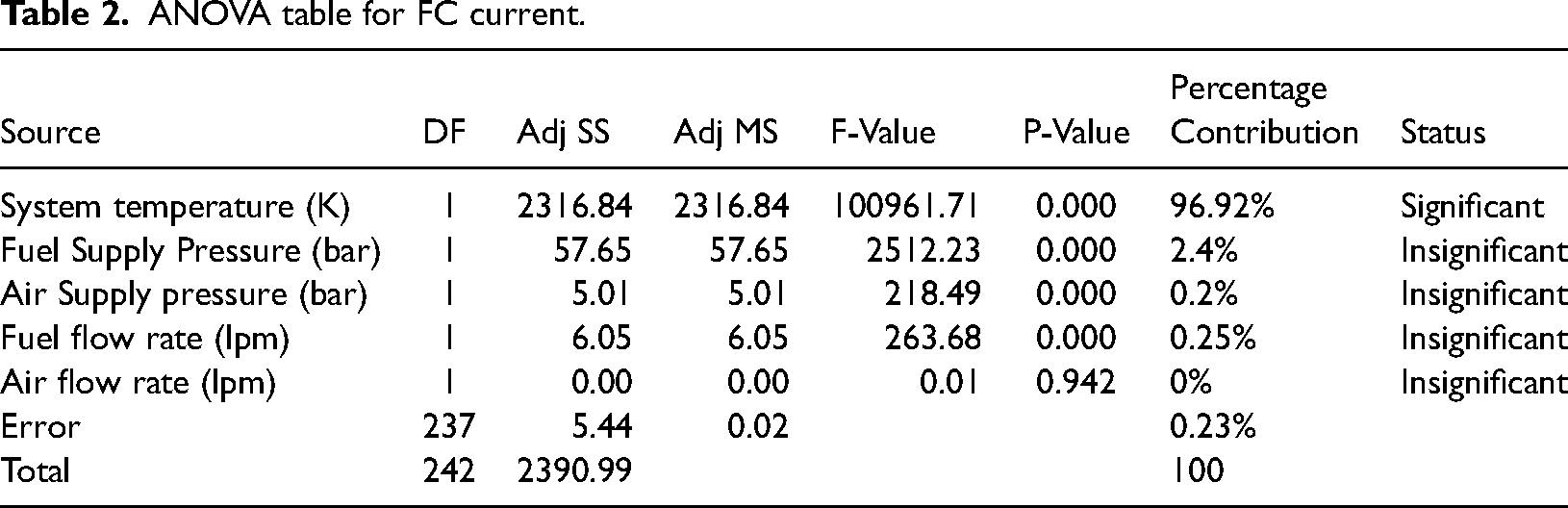
Regression equation of fuel cell current is developed using Minitab in terms of system temperature, fuel supply pressure, air supply pressure, fuel flow rate and air flow rate and also ANOVA table is also generated using Minitab to find the significant parameter on fuel cell current which is shown in Table 2. It is clearly observed that the system temperature has significant percentage contribution as 96.92% compared to other parameters.
ANOVA table for FC current.
FC current = -23.216 + 0.126058 System temperature (K)
+ 1.1931 Fuel Supply Pressure (bar)
+ 0.3519 Air Supply pressure (bar) + 0.03433 Fuel flow rate (LPM)
+ 0.000001 Air flow rate (LPM)
Regression analysis: FC voltage (V)
Regression equation of FC voltage is developed using minitab in terms of system temperature, fuel supply pressure, air supply pressure, fuel flow rate and air flow rate and also ANOVA table is also generated using Minitab to find the significant parameter on fuel cell current which is shown in Table 3. It is clearly observed that the system temperature has significant percentage contribution as 86.22% compared to other parameters.
ANOVA table for FC voltage.
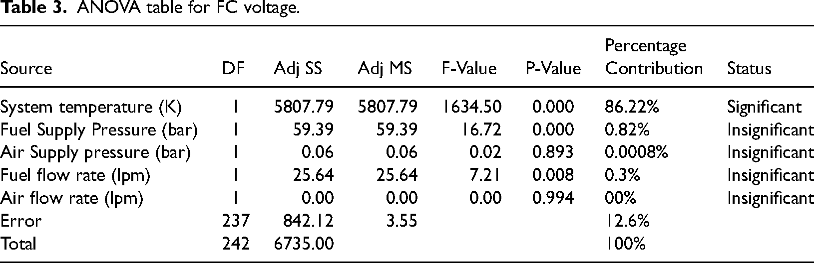
Fuel cell voltage (V) = -33.95 + 0.19958 System temperature (K)
+ 1.211 Fuel Supply Pressure (bar) - 0.040 Air Supply pressure (bar)
+ 0.0707 Fuel flow rate (lpm) + 0.000001 Air flow rate (lpm)
Machine learning model selection
There are broadly two types of MLAs, supervised and unsupervised algorithms. They differ in the way the training data and the way the models are trained. Supervised MLAs are used when there is labelled data which contains both input and output. The algorithm learns the representation between the input and the output variables so that it can be used to classify new and unseen datasets and predict outcomes. Supervised MLAs are usually used to classify items or forecast values. Unsupervised MLAs are used where the training data is unlabelled and has only input data. The algorithm learns the representation of the data without any interference from humans and comes up with its own insights. Unsupervised machine learning algorithms are used to cluster similar data into similar groups.
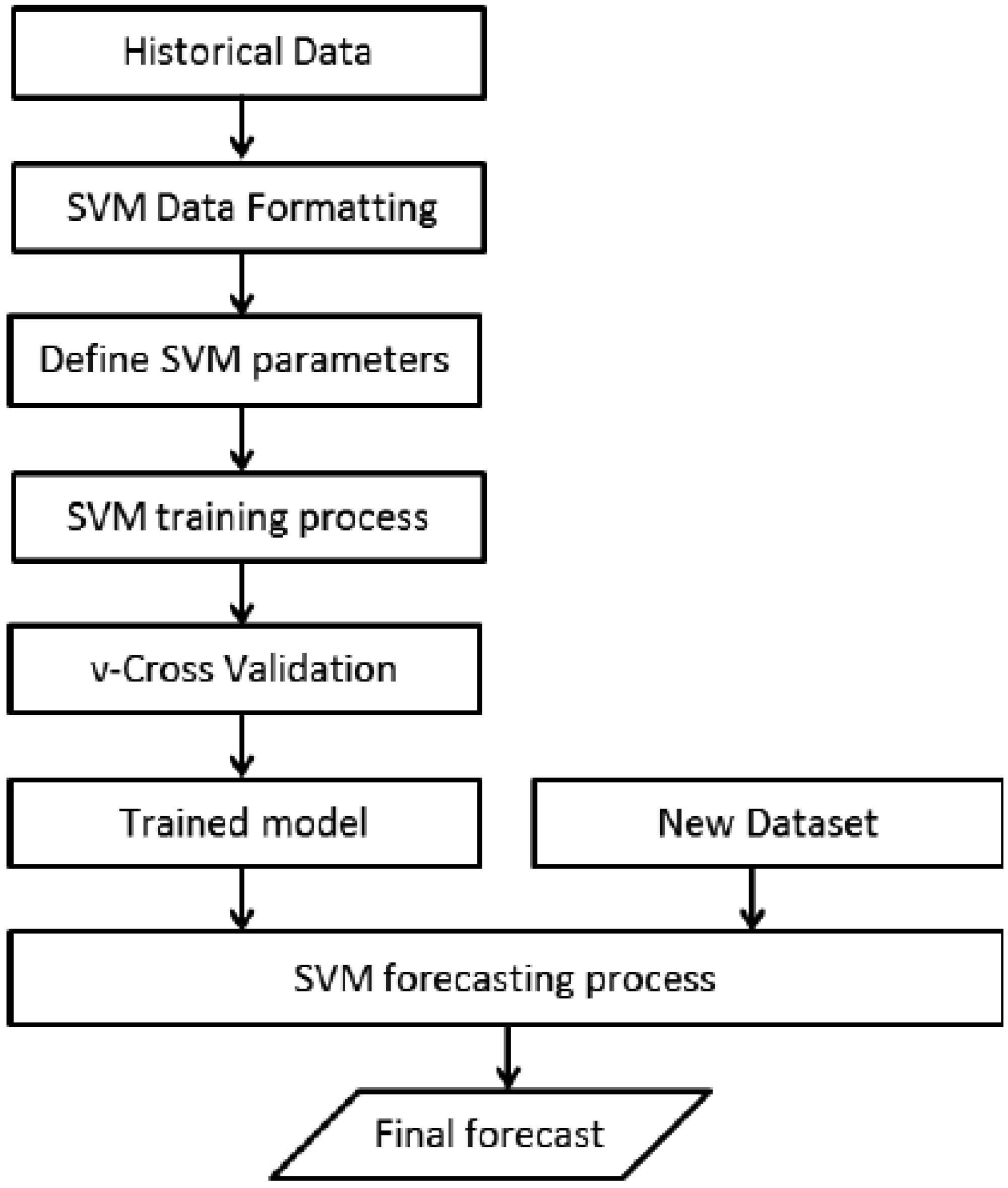
In this scenario, data from PEM experiments have input parameters such as system temperature, fuel supply pressure, air supply pressure, fuel flow rate and air flow rate to measure the output parameters like FC current, FC voltage and FC output power. Since both the input and the output parameters are there, Supervised MLAs can be used to learn the representation of the input parameters to the output parameters. The working model of the MLAs is explained using a flowchart which is shown in Figure 6.
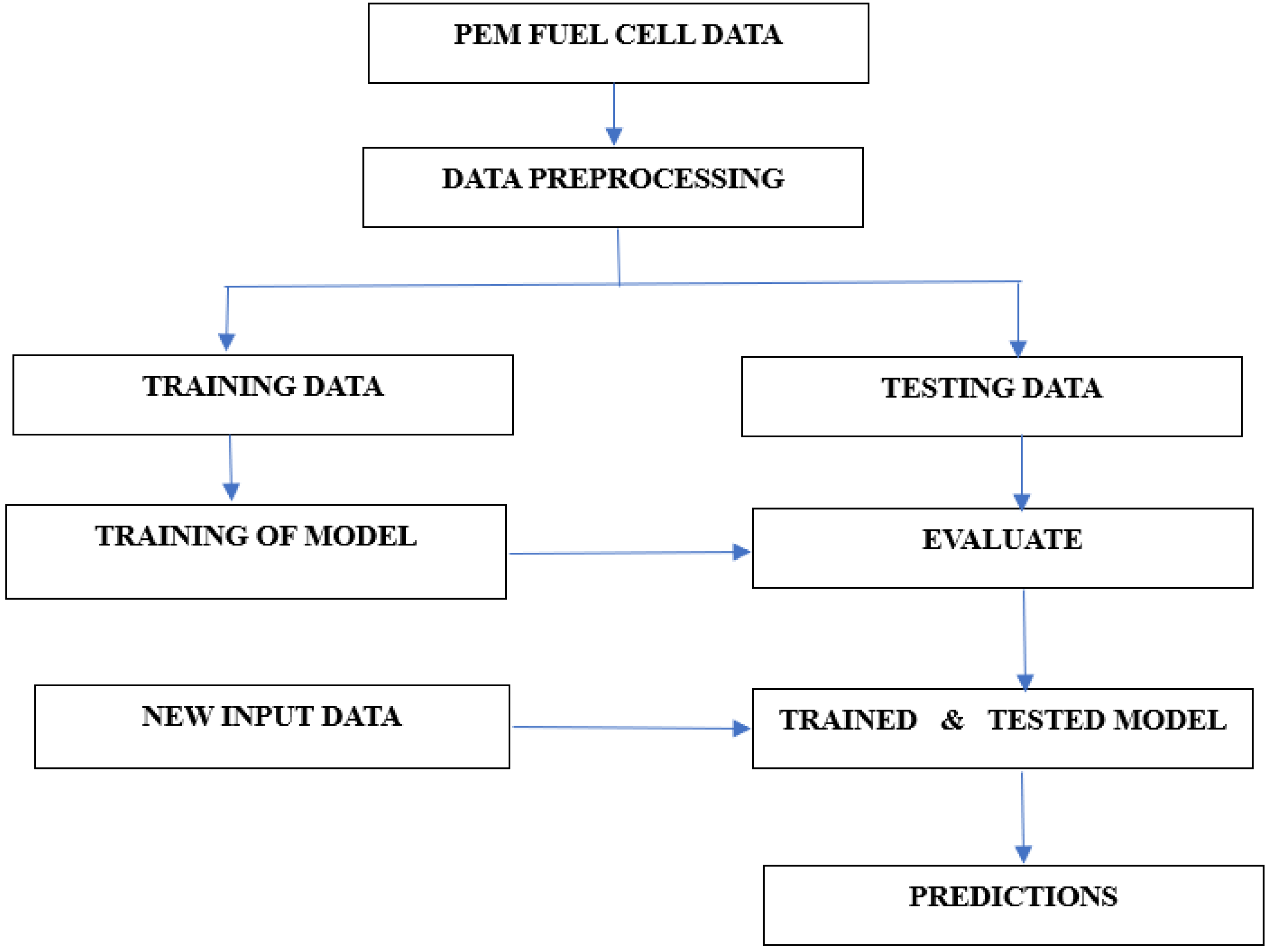
Supervised ML flowchart.
GBR method.
Assumptions made for modeling of MLAs are
The supervised regression algorithms are suitable only to find linear and non linear interactions of input and output parameters, it may not be accurate for more complex, higher order interactions between the input and output parameters. It is assumed that the data measured is comprehensive and free from noise, it may leads to inaccurate predictions It is assumed that the operating conditions of the PEMFC remail stable, it may not give highly dynamic environments.
Supervised MLAs
Supervised MLAs are classified into two categories based on the type of response data such as classification and regression. Classification algorithms predict a discrete output value based on the input variables and can be used when the target variable is a discrete value like if the weather is going to be sunny or not, or if the image is a dog or a cat. Regression algorithms predict a continuous output value based on the input variables and it can be used when the target variable is a continuous quantity like income, scores, height or weight. Since output data in this study comprises continuous output variables, Regression algorithms are used to predict the output values. There are multiple regression algorithms that have been developed and each algorithm has its pros and cons. (Fathy, Abdel Aleem and Rezk, 2021) used different machine learning algorithms such as linear regression, K nearest neighbor algorithm, ANN, decision tree and Bayesian learning for different applications are discussed. In this study, multiple regression algorithms are compared to check which is the best one for predicting PEM voltage and current.
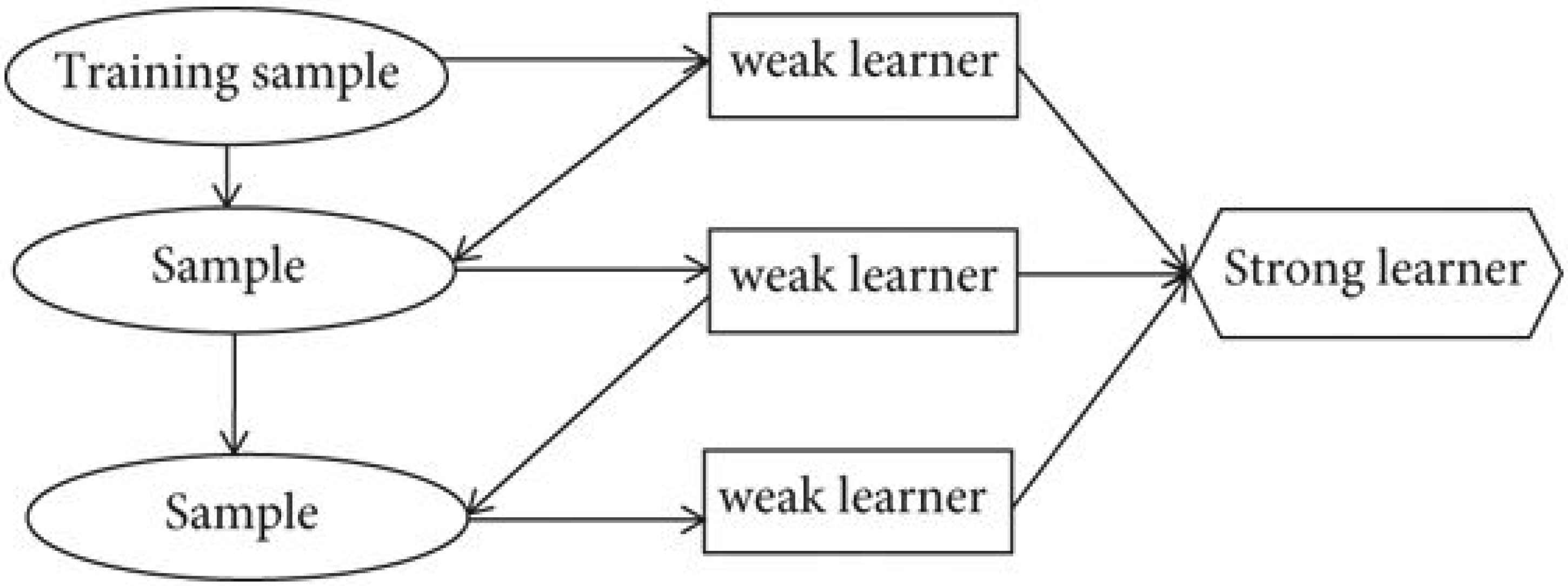
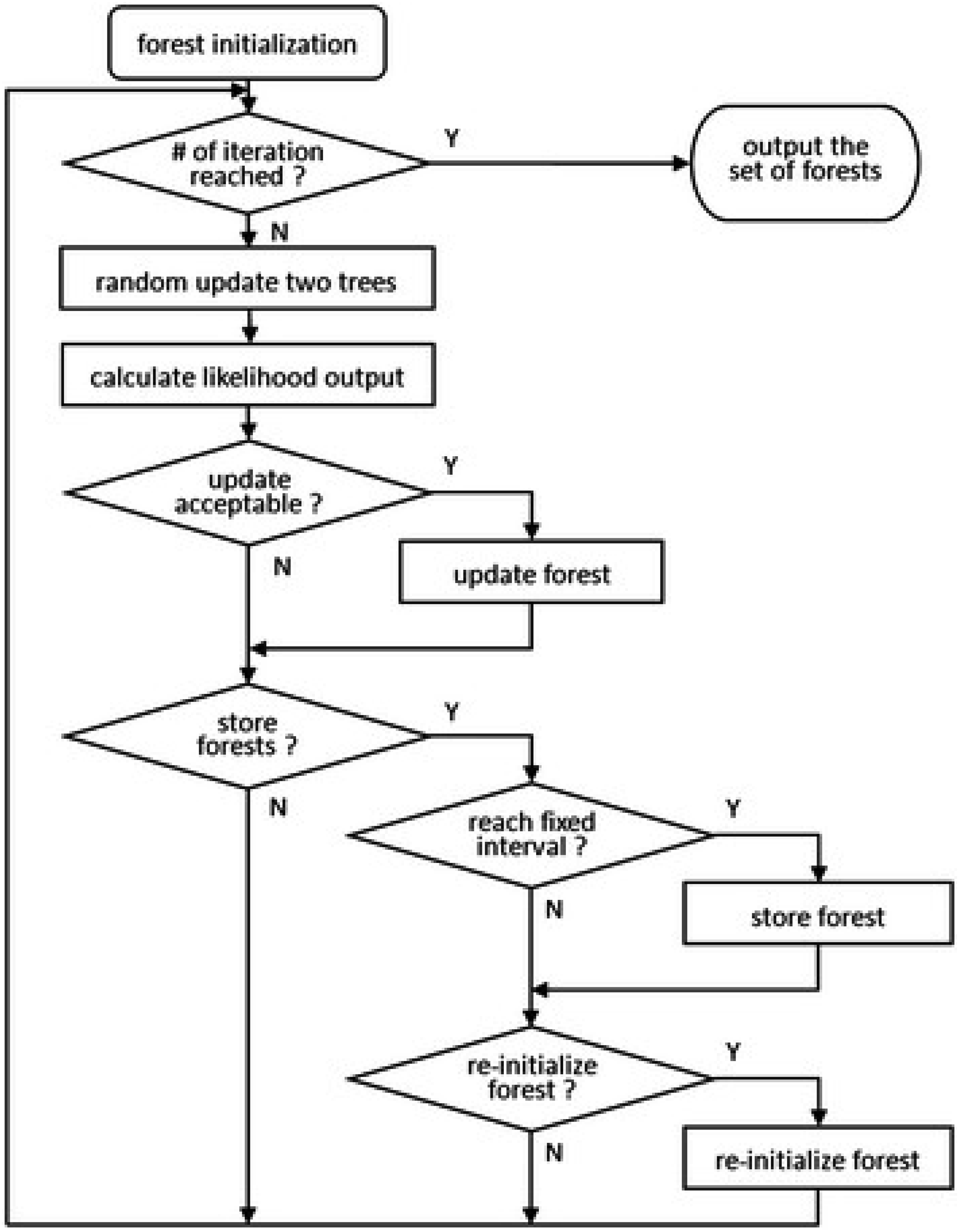
Gradient boosting regression (GBR)
A GBR is a regression model which creates many small models and combines them into a single model for obtaining better performance as a single model as seen in Figure 7. Each small model is trained to reduce the loss function in terms of mean squared error (MSE) or gradient-based cross-entropy of the previous model. In every iteration gradient loss function will be computed with respect to current predictions and then the new model with a lesser gradient loss function. Then the predictions of the new model will be added to the current model and this process will be repeated n number of times to achieve the best model.
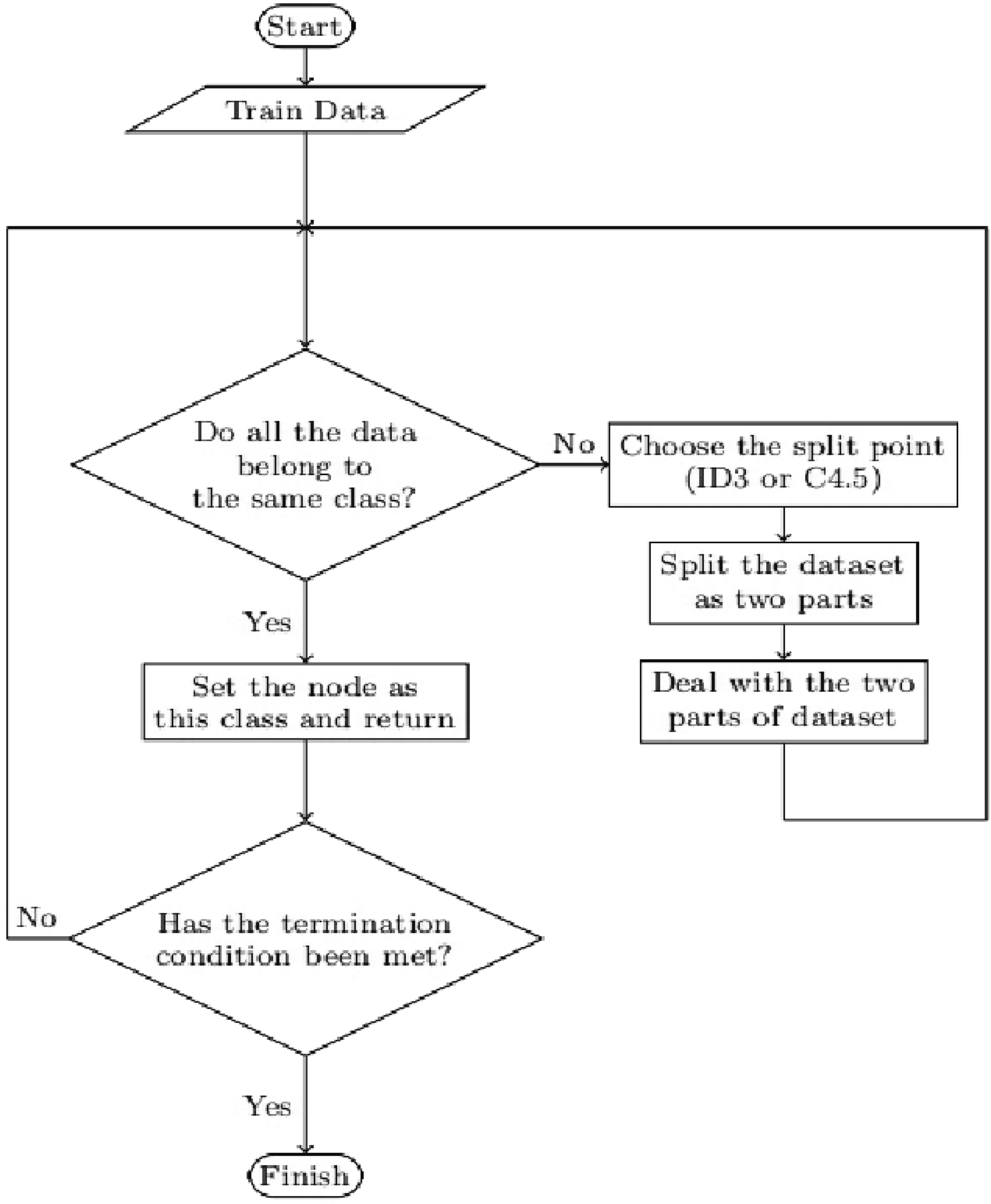
Decision tree regression
A decision tree regressor creates a tree-like structure which is used to predict the output value shown in Figure 8. This tree-like structure is developed by breaking the data set into smaller sets of data and incrementally creating a tree-like structure. The final decision tree model with decision and end nodes which used to predict the target value.
Decision tree regression.
Random forest regression
Multiple decision trees will be combined to create a random forest regressor model which is shown in Figure 9. Basically, it is a training of different decision tree models on the same training data and finally average of all the results will reduce the errors which improves the performance of an algorithm.
Random forest regression.
Support vector regression (SVR)
SVR develops a hyperplane which fits the data into the continuous space shown in Figure 10. It is obtained by mapping all input points into a high-dimensional feature space and trying to increase the distance between the hyperplane and closest points which leads to minimum error. SVR can handle inputs and output with nonlinear relations by using the different kernel functions to map with high dimensional space.
SVR method.
Regression metrics
R-squared value
R-squared value is a post metric which is used to calculate the coefficient which is a percentage of total variance in output explained by the variance in input. It gives the good fitness of any regression model and explains the difference between predicted and actual output values. The ideal value of R² is one or close to one which can be obtained by a lesser sum of squared error of the regression line and means that the model is able to find the 100 percent variance in the output variable. The worst value of R² is zero or close to zero which can be obtained by a higher sum of squared error of the regression line and means that the model is not able to find any variance in the output variable
Mean absolute error (MAE)
MAE is an average value of differences between predicted and actual output values. It is robust to outliers because it gives direct error which is not exaggerated and is used to measure deviations of predictions from the actual output values. It gives only the absolute value of the residual, but the direction of error is not considered which leads to under or over-prediction of output values.
Mean square error (MSE)
MSE is an average value of squared differences between predicted output values by the regression models and actual output values. It is differentiable and even small errors are penalized by squaring leading to the overestimation of errors which exaggerates the badness of the model.
Root mean squared error (RMSE)
RMSE is the square root of the average value of the squared difference between output values by the regression models and actual output values. Differential property of mean squared error is retained and small errors are penalized by square rooting of errors. Outliers can be handled with less struggle in RMSE due to the smooth interpretation of error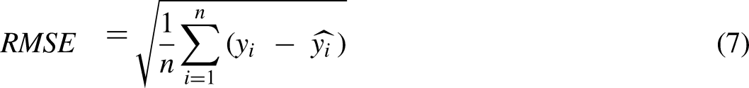
Modelling and testing
243 experimental values of the PEMFC are considered for the modelling of the gradient boosting algorithm. There are five input attributes system temperature (K), fuel supply pressure (bar), air supply pressure (bar), fuel flow rate (lpm) and air flow rate (lpm) and two output attributes such as FC current (A) and FC voltage (V) are considered for training and testing. As the first step, the entire data is split into two categories such as training data which is used to train a model and testing data which is used to measure the performance of the algorithm. In this paper out of 253 data sets 80% of the data is used for training and 20% of the data is utilized for testing of an algorithm. Python scikit learn module is used for the modelling of the algorithms and also to measure the accuracy of the algorithm. After training and testing, Models can be used for the predictions and the same will be verified with experimentation trials.
Gradient boosting regressor (GBR)
The modelling of the GBR model is performed and the performance metrics are measured and seen in Table 4. The FC current and voltage are modelled using the GBR algorithm by training data and then predicted via testing data input attributes. The predicted values are compared with the actual output from the testing data and plotted in Figure 11.
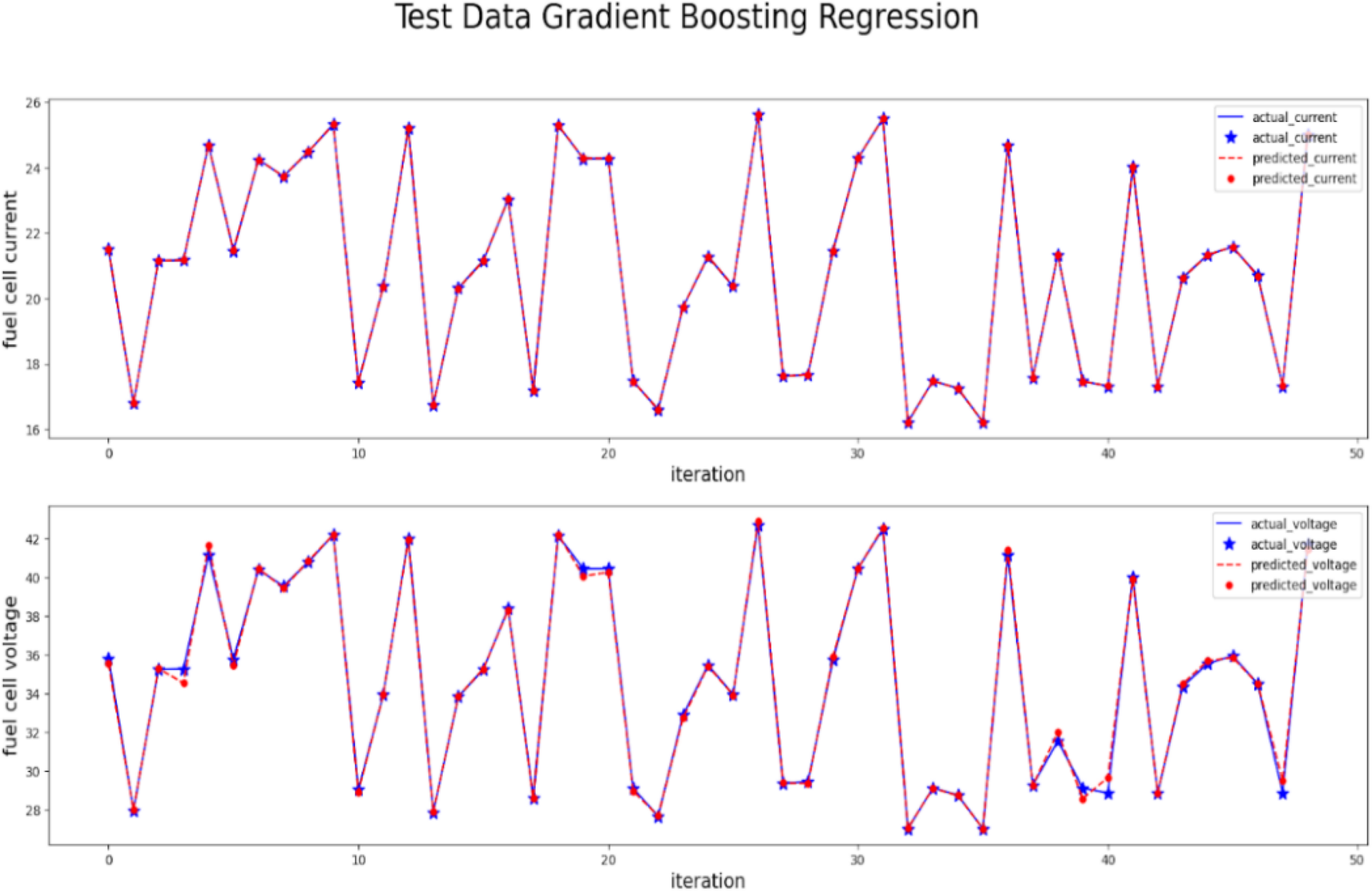
Actual vs predictions by gradient boosting.
Regression metrics of gradient boosting.
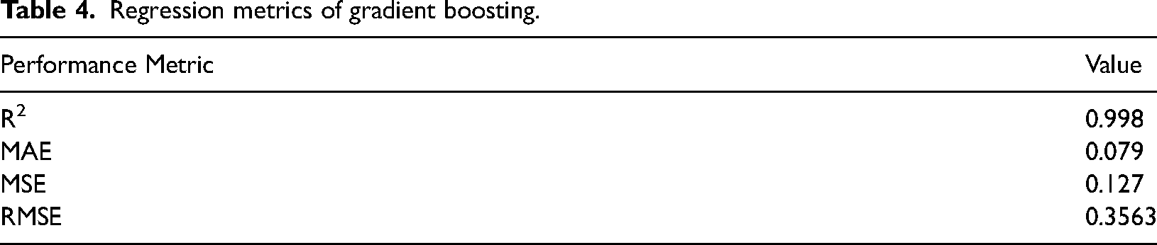
It is observed that predicted values are merged with actual values in the majority of the points and only very few points are not in line with actual values which proves the fitness of the model with actual data. The quality of the model is measured using different metrics such as R-squared, MAE, MSE and RMSE values. The gradient boosting model has an R2 value of 0.998 which is very close to one, errors such as MAE 0.079, MSE 0.127 and 0 RMSE value prove the good fitness of the regression model.
Decision tree regressor (DTR)
The modelling of the DTR model is performed and the performance metrics are measured and seen in Table 5. The FC current and voltage are modelled using the DTR by training data and then predicted via testing data input attributes. The predicted values are compared with the actual output from the testing data and plotted in Figure 12.
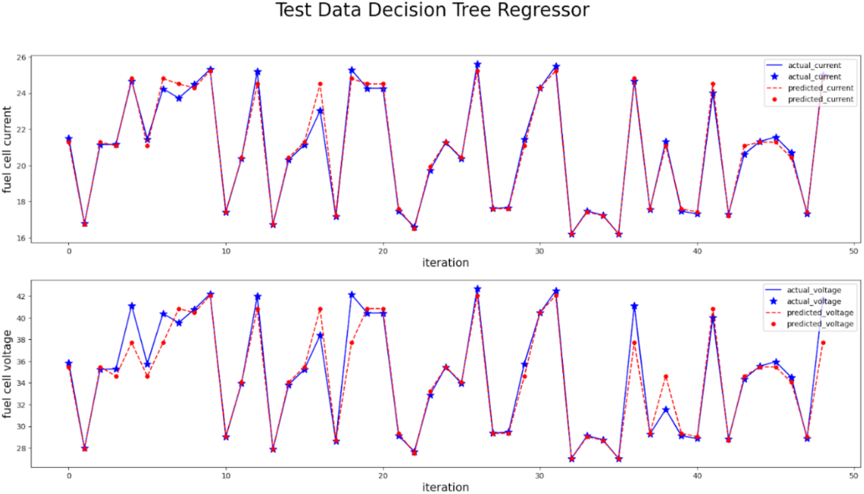
Actual vs predictions by DTR.
Regression metrics of decision tree.
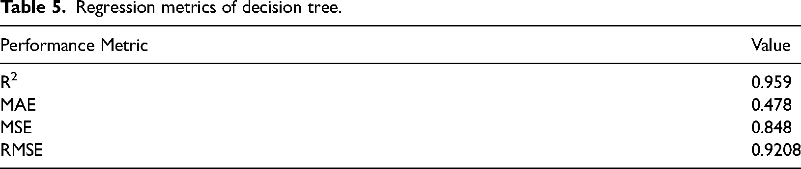
It is observed that predicted values are merged with actual values in the majority of the points but a few points are not in line with actual values. Observations are made clear that the Prediction of high voltage and current points are deviated more compared to less current and voltage values and actual values are always higher than the predicted value. The quality of the model is measured using different metrics such as R-squared, MAE, MSE and RMSE values. The decision Tree model has an R2 value of 0.959 which is very close to one, errors such as MAE 0.478, MSE 0.848 and 0.0006 RMSE value prove the better fitness of the regression model.
Random forest regression (RFR)
The modelling of the RFR model is performed and the performance metrics are measured and shown in Table 6. The FC current and voltage are modelled using the RFR algorithm using training data and then predicted using testing data input attributes. The predicted values are compared with the actual output from the testing data and plotted in Figure 13.
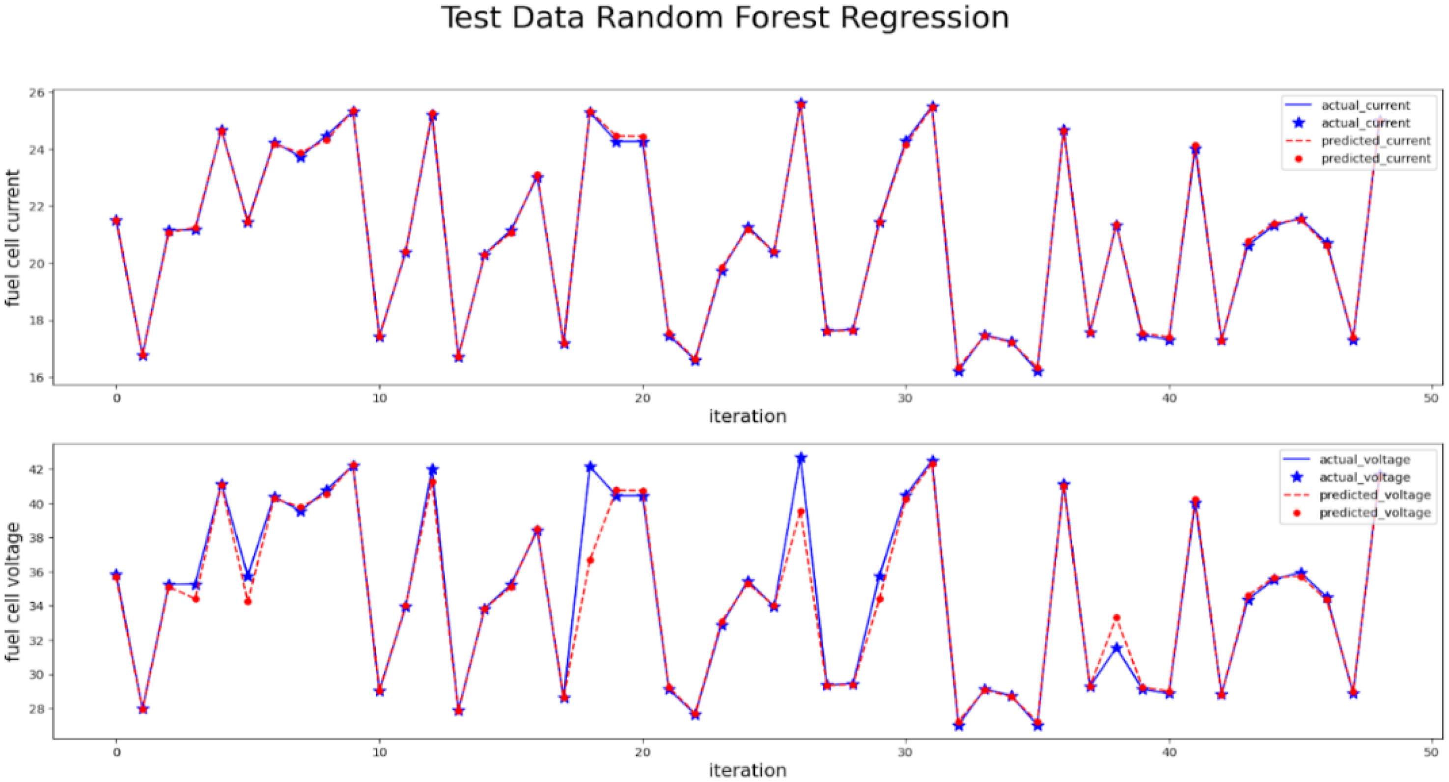
Actual vs predictions by RFR.
Regression metrics of random forest.

It is observed that predicted values are merged with actual values in the majority of the points but a few points are not in line with actual values. Observations are made clear that the prediction of high voltage and current points are deviated more compared to less current and voltage values and actual values are always higher than the predicted value. The quality of the model is measured using different metrics such as R-squared, MAE, MSE and RMSE values. The random forest model has an R2 value of 0.981 which is very close to one, Errors such as MAE 0.235, MSE 0.154 and 0.0003 RMSE value prove the better fitness of the regression model.
Support vector regression (SVR)
The modelling of the SVR model is performed and the performance metrics are measured and shown in Table 7. The FC current and voltage are modelled using the SVR algorithm using training data and then predicted using testing data input attributes. The predicted values are compared with the actual output from the testing data and plotted in Figure 14.
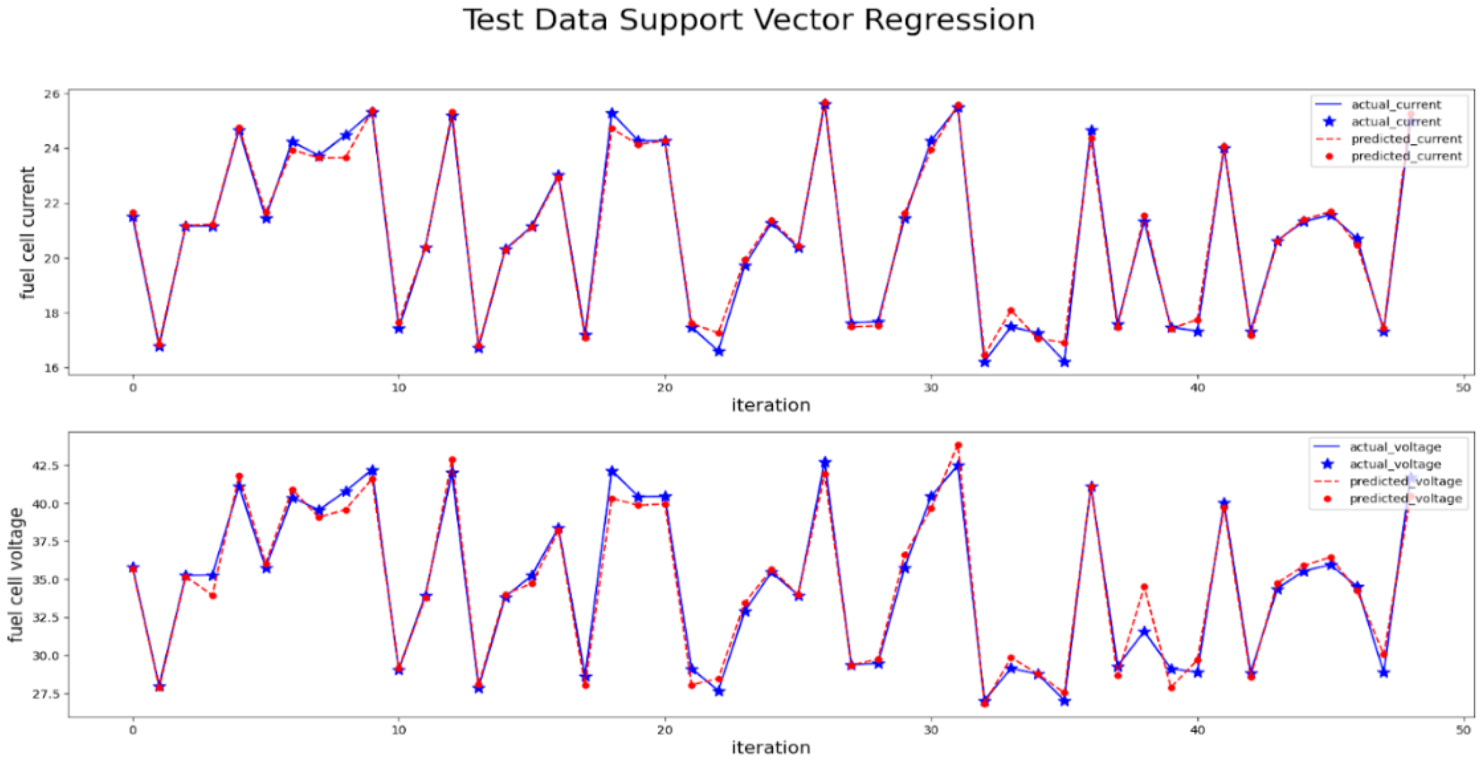
Actual vs predictions by SVR.
Regression metrics of SVR.
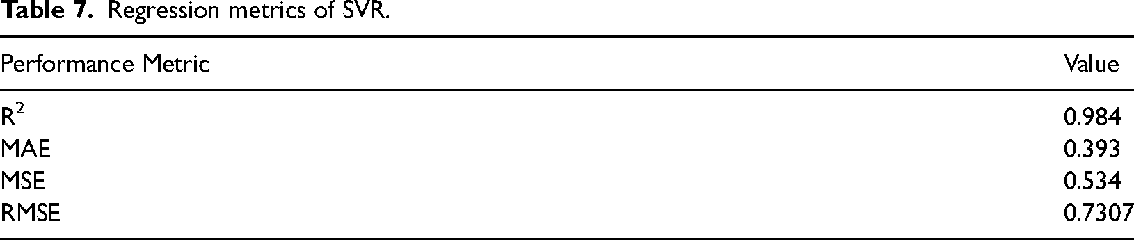
It is observed that predicted values are merged with actual values in the majority of the points but a few points are not in line with actual values. Observations are made clear that prediction of peak values voltage and current points are deviated more compared to other value predictions. The quality of the model is measured using different metrics such as R-squared, MAE, MSE and RMSE values. The SVM model has an R2 value of 0.984 which is very close to one, errors such as MAE 0.393, MSE 0.534 and 0.0003 RMSE value prove the better fitness of the regression model.
The parity plots for different machine learning algorithms are shown in Figure 15 and blue color points represents predicted current values and red color points represents predicted voltage values. The points cluster around the diagonal line represents the deviation between the experimental and predicted values. In SVR predictions, a greater number of both red and blue points away from the diagonal line which indicates the less accuracy in predictions. In decision tree parity plot, it is observed that a few points are away from the diagonal line which means, decision tree predictions are better compared to SVM algorithm. In random forest algorithm one or two points are far from the line which indicates random forest algorithm predicts more accurately compared to SVM algorithm and decision tree algorithm. Finally, it is proved that gradient boosting algorithm predictions have highest accuracy compared to all other three algorithms because not even single point is out of diagonal line in gradient boosting parity plot.

Parity plots of MLAs.
Results of MLAs
Supervised MLAs regression considered in this paper are gradient boosting regression, decision tree regressor, random forest regression and support vector regression and python coding is used for the modelling and analysis of algorithms. Estimate parameters for different MLAs for the PEMFC dataset are given in Table 8 and represented as a bar chart which is shown in Figure 16.
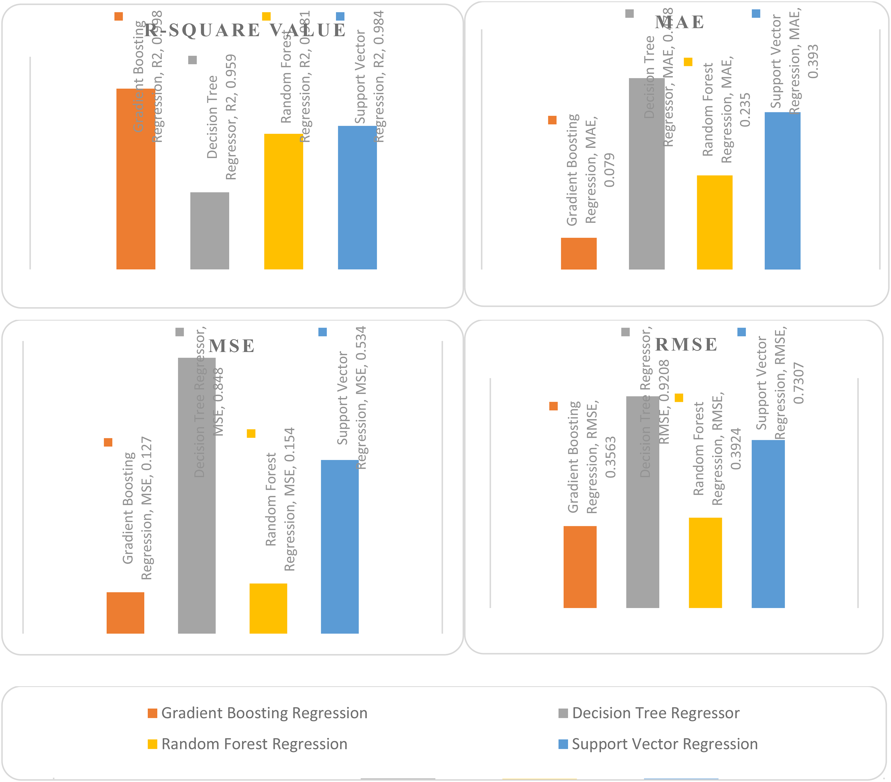
Performance estimate of MLAs.
Performance estimate of machine learning algorithms of PEM fuel cell dataset.
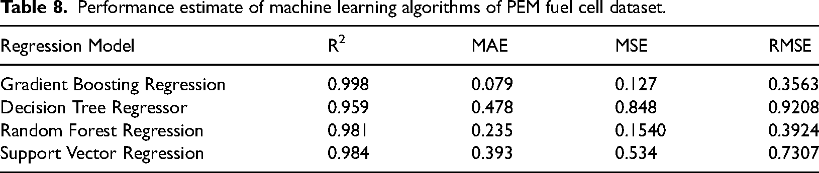
For the effective estimation of PEM FC data, R2, MAE, MSE and RMSE are considered as evaluation metrics for the MLAs which are shown in Table 5. By the interpretation of the estimation measure values from Table 5 and Figure 16, it is proved that the gradient boosting regressor gives accurate prediction compared to the RFR, decision tree regressor and SVR. Better models can be obtained by the lesser values of errors such as MAE, MSE and RMSE values which lead to better R-squared values which is closer to one. In the above study, the gradient boosting regression algorithm has the R-squared value of 0.998 which is very close to one and lesser error values (MAE, MSE &RMSE) which means accurate prediction of output measures is possible.
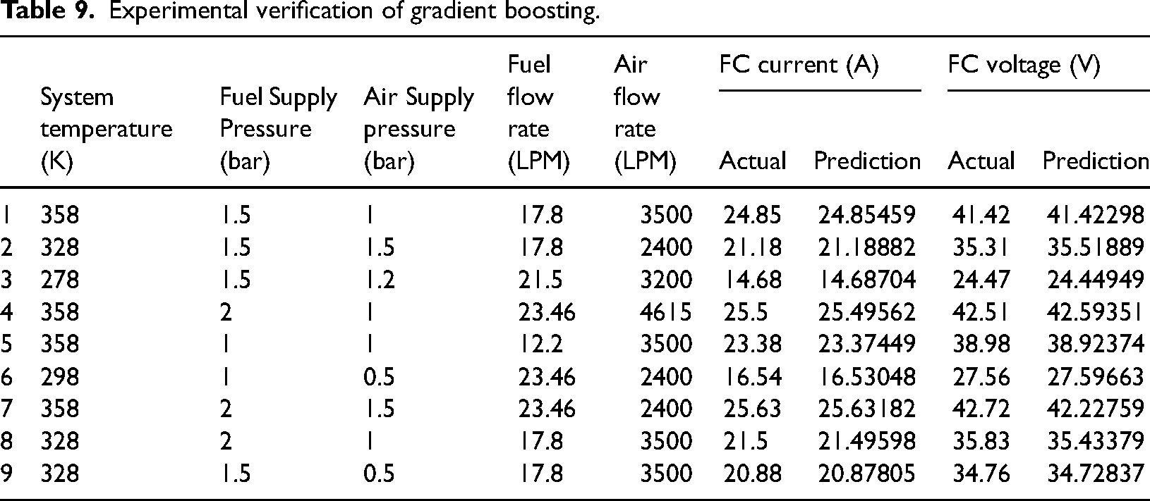
By comparing the entire algorithms gradient boosting algorithm gives the best results which are selected for the PEM FC current and voltage prediction. Now there are nine different combinations of input parameters are chosen for the experimental verification of the gradient boosting algorithm. Actual PEM FC current and voltage are measured and compared with the gradient boosting predictions which are shown in Table 9. Almost predicted all values are exactly matching with the experimental values. The model is generally reliable when predictions fall within expected ranges, and confidence intervals are tight. The gradient boosting model is generally reliable within the operating conditions it was trained on, but its performance may degrade under extreme or unseen conditions. To ensure robust predictions across a wide range of scenarios, it is important to test the model on data outside the training range, assess its uncertainty, and potentially update or augment the model with additional data or complementary methods.
Experimental verification of gradient boosting.
This paper quantifies the impact of key parameters on PEMFC performance using machine learning techniques. The higher prediction accuracy of gradient boosting regression algorithm proves its potential as a powerful algorithm for real time optimization and also in control of PEMFC in practical applications. This study not only increasing the understanding the PEMFC characteristics under various operating conditions but also offers a pathway for enhancing the efficiency and reliability of fuel cells in transportation and other energy-intensive sectors.
Limitations of this study are, these models are developed for specific PEMFC configurations, their applicability to different PEMFC designs or operating environments may be limited., the accuracy of prediction is limited by the quality and quantity of the available data and External factors such as environmental conditions, aging effects of the fuel cell, and material degradation over time were not included in the analysis. The Gradient Boosting model's performance on different types or sizes of PEM cells and its transferability to other fuel cell systems depend on several factors, including the diversity and representativeness of the training data, the adaptability of the model, and the relevance of the features.
Conclusion
In this paper, the performance of power generation using PEM-FC is improved using data analysis techniques such as GBR, DTR, SVR and RFR.
Highlights of this research work:
The most significant operating parameter of PEM-FC is found by conducting regression analysis. Different machine learning models used for prediction of optimum operating parameters to maximize the performance. The gradient boosting algorithm yields betters results than other models in predicting PEM fuel optimum operating parameters. The experimental validation is also carried out to validate the results obtained from machine learning models. The model is generally reliable when predictions fall within expected ranges, and confidence intervals are tight. The GBR model is generally reliable within the operating conditions it was trained on, but its performance may degrade under extreme or unseen conditions. To ensure robust predictions across a wide range of scenarios, it is important to test the model on data outside the training range, assess its uncertainty, and potentially update or augment the model with additional data or complementary methods which will be the scope of this study.
Footnotes
Acknowledgment
The authors extend their appreciation to the deanship of Scientific Research at King Khalid University, Abha, KSA, for funding this work through the research groups program under grant number (RGP.2/594/44).
Data availability
The data used to support the findings of this study are available from the corresponding author upon request.
Declaration of conflicting interests
The authors declared no potential conflicts of interest with respect to the research, authorship, and/or publication of this article.
Funding
The authors received no financial support for the research, authorship, and/or publication of this article.