Sage Journals: Discover world-class research

Abstract

Accurate identification of water-inrush sources is critical for deep mining safety. This study proposes an entropy-weighted variable fuzzy set (EW-VFS) model, which uses information entropy to objectively determine the importance of different hydrochemical indicators, to discriminate complex mixed water sources in the Sunzhuang Minefield, North China. In this study, we analyzed 86 water samples from five key aquifers—Permian sandstone fractured aquifers, Ordovician limestone karst aquifers, and three thin-layer limestone aquifers—using nine hydrochemical parameters. Entropy weight analysis identified Mg²⁺ and HCO₃⁻ as the dominant indicators for source discrimination. The EW-VFS model achieved an overall accuracy of 83.33%, demonstrating high reliability, particularly for Permian sandstone fractured water and Ordovician limestone water. Furthermore, a time-series analysis of the model's rank feature value (H_i) revealed a dynamic evolution of the inrush source, showing a clear transition between different thin-layer limestone aquifers during mining operations. This study's findings demonstrate the model's utility in identifying multisource water inrush. However, its performance in differentiating the highly similar thin-layer limestone aquifers shows potential for further enhancement, which could be addressed with more comprehensive hydrogeochemical data.

Keywords

Deep mining hydrogeology multi-aquifer mixing water source identification rank feature value mine water hazard prevention

Introduction

As one of the world's largest energy consumers, China has long maintained a coal-dominant energy consumption structure (Wu et al., 2024). To ensure stable coal supply, mining operations are progressively extending to greater depths (Yang et al., 2021). Under deep mining conditions, coal seams intersecting with multiple aquifers fundamentally alter natural groundwater flow paths, water-rock interactions, and hydrogeological structure (Hou et al., 2024). Mining-induced disturbances and high-pressure karst water cause extensive fractures in the surrounding rock. These disturbances can also activate faults and collapse columns, forming new water-conducting channels. This creates favorable conditions for groundwater inrushes into coal mining faces, severely threatening operational safety (Chen et al., 2023) and concurrently leading to environmental degradation, including groundwater depletion, water quality deterioration, and surface subsidence (Wang et al., 2022). These challenges are exacerbated under complex hydrogeological conditions involving great mining depths and high-pressure karst water, which often result in dispersed water-inrush points and mixed water sources (Hamed et al., 2011). Therefore, in the event of a water inrush, accurately identifying the source is the primary task for formulating effective control measures (Wang et al., 2019). This task is of critical importance for both ensuring mining safety and managing water resources sustainably (Yang et al., 2021).

To address water-inrush source discrimination in multi-aquifer systems under deep mining conditions, extensive studies have been conducted using hydrogeochemical characteristics, isotopes, trace elements, and hydrogeochemical modeling (Aris et al., 2007; Chen et al., 2011; Qian et al., 2018; Yang et al., 2021; Yu et al., 2022). These studies highlight the importance of vertical hydrogeochemical heterogeneity in deep mining. This characteristic provides a reliable foundation for distinguishing aquifers, understanding their hydraulic connections, and identifying water-inrush sources (Qu et al., 2023; Wang et al., 2024). However, with increasing mining depth and scale, aquifer mixing intensifies, leading to more similar hydrogeochemical signatures. Consequently, relying solely on these characteristics becomes insufficient for accurately identifying the sources and contribution ratios of mixed water inrushes (Chen et al., 2022). To overcome this limitation, researchers have begun to integrate multivariate statistical methods with hydrogeochemical data to establish more robust mathematical models for water source discrimination. For example, by integrating the complementary advantages of the Analytic Hierarchy Process (AHP) and Grey Relational Analysis (GRA), researchers developed a predictive model for comprehensive evaluation of roof water-inrush risks (Zhang et al., 2019). Chen and Gui (2021) used the Fisher discrimination model to identify inrush water sources based on five conventional hydrogeochemical parameters and δ¹⁸O-δD isotopic data from water samples. Principal component analysis (PCA) and Bayesian multiclass linear discriminant analysis (LDA) were employed to discriminate among four aquifer types (Xue et al., 2023). A fuzzy comprehensive evaluation model was developed using 18 water sample indicators, accurately determine the primary sources of total mine water discharge (Xu et al., 2018). Based on hydrogeochemical data, Huang et al. (2017) developed a water source identification model by combining Fisher discriminant analysis and gray correlation theory (Huang et al., 2017). While these combined statistical and mathematical models show advantages in processing large datasets (Belkhiri et al., 2010), they exhibit significant limitations when applied to the complex hydrogeological conditions of deep mining, where aquifer mixing is prevalent. For instance, Bayesian models are highly sensitive to static prior probabilities, which may become unreliable as mining activities dynamically alter groundwater chemistry (Zhang et al., 2020b). Gray relational models depend on preset reference sequences, limiting their adaptability to parameter shifts caused by aquifer mixing (Yang et al., 2023). More critically, existing fuzzy models lack the adaptability to parameter shifts caused by aquifer mixing (Liu et al., 2017). They typically employ rigid membership functions with fixed shapes and ranges, rendering them incapable of responding to the changing parameter distributions that result from mining disturbances (Wang et al., 2018). Therefore, a clear knowledge gap exists for a discrimination model that can dynamically adapt to the fuzzy and variable nature of mixed water sources under deep mining-induced stress. Developing such a flexible and robust model is the primary objective of this study.

To address this gap, this study proposes a novel Entropy Weight-Variable Fuzzy Set (EW-VFS) model and applies it to the Sunzhuang Minefield in the Fengfeng mining area (Figure 1). This approach first utilizes the entropy weight method to objectively determine the weights of different hydrogeochemical discrimination indicators (Chen, 2005). These weights are then integrated into a variable fuzzy set framework to build the discrimination model (Wang et al., 2019). The model identifies water-inrush sources by calculating the comprehensive relative membership degree of a water sample to each potential aquifer and classifying it based on the principle of maximum membership and rank feature values (Chen, 1993). By dynamically adapting to the fuzzy characteristics of mixed water, the proposed EW-VFS model demonstrates enhanced flexibility and discrimination accuracy, providing a robust new methodology for water source identification under complex deep-mining conditions.

Figure 1.

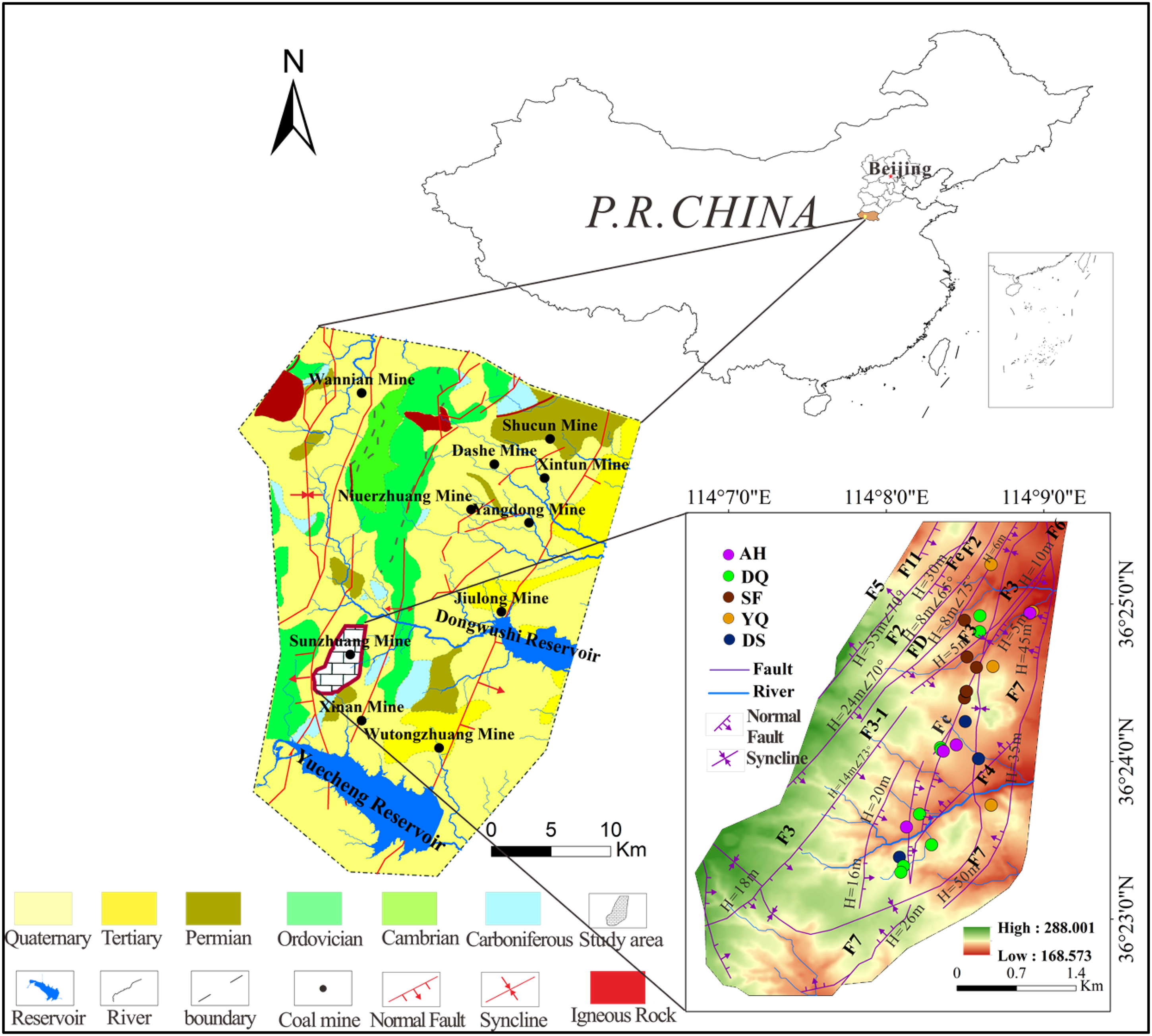
Overview of the study area and sampling point distribution.

Hydrogeological conditions of the study area

The Fengfeng mining area, a critical energy and industrial base in North China, is located in southwestern Handan City, Hebei Province, as a part of the Handan-Xingtai hydrogeological unit (Qu et al., 2018). Over half a century of intensive mining has significantly altered the in situ stress, displacement, seepage, and hydrogeochemical fields of the surrounding rock, leading to complex hydrogeological conditions and frequent water-inrush incidents (Zhang et al., 2022). Sunzhuang Minefield has achieved a peak annual output of 120 Mt. Its operations, which mine three main coal seams at depths down to approximately −500 m, face significant water-inrush threats from multiple aquifers. Previous research on this minefield has predominantly focused on prevention measures against Ordovician limestone confined water (Sun et al., 2019; Hao et al., 2021; Kai et al., 2023). Limited studies have investigated vertical hydraulic connections among multiple aquifers or water-inrush source identification. Particularly, thin-layer limestone aquifers have often been treated as generalized units without further subdivision in most existing studies (Guo et al., 2017; Sun et al., 2023).

The Sunzhuang Minefield, located in the southwestern part of the mining area, is characterized by low mountainous and hilly topography, with elevations ranging from +288 to +168 m and a general slope from southwest to northeast. During deep mining operations, three major water-inrush aquifer types are encountered: (1) Quaternary weathered bedrock porous aquifers, (2) Permian sandstone fractured aquifers, and (3) Carboniferous and Ordovician limestone karst-fractured aquifers. Years of hydrogeological exploration and mining exposure have revealed nine distinct aquifers from top to bottom (Figure 2). The Quaternary weathered bedrock aquifer and Shihezi sandstone aquifer are excluded from this study as they exhibit weak water-bearing properties and maintain considerable distances from working faces during deep mining operations. The Permian sandstone aquifer primarily consists of the Shanxi Formation fractured sandstone aquifer. The Carboniferous limestone karst-fractured aquifers include five subunits: Yeqing limestone, Shanqing limestone, Fuqing limestone, Xiaoqing limestone, and Daqing limestone aquifers. Due to their spatial contiguity and hydrogeochemical consistency, the Shanqing and Fuqing limestone aquifers are combined into a single unit, the Shanfuqing limestone aquifer. The Xiaoqing limestone aquifer is excluded from this study due to its weak water yield capacity. The Ordovician limestone karst aquifer, which forms the bedrock of the coal seams, exhibits an exceptionally strong yet heterogeneous water yield capacity.

Figure 2.

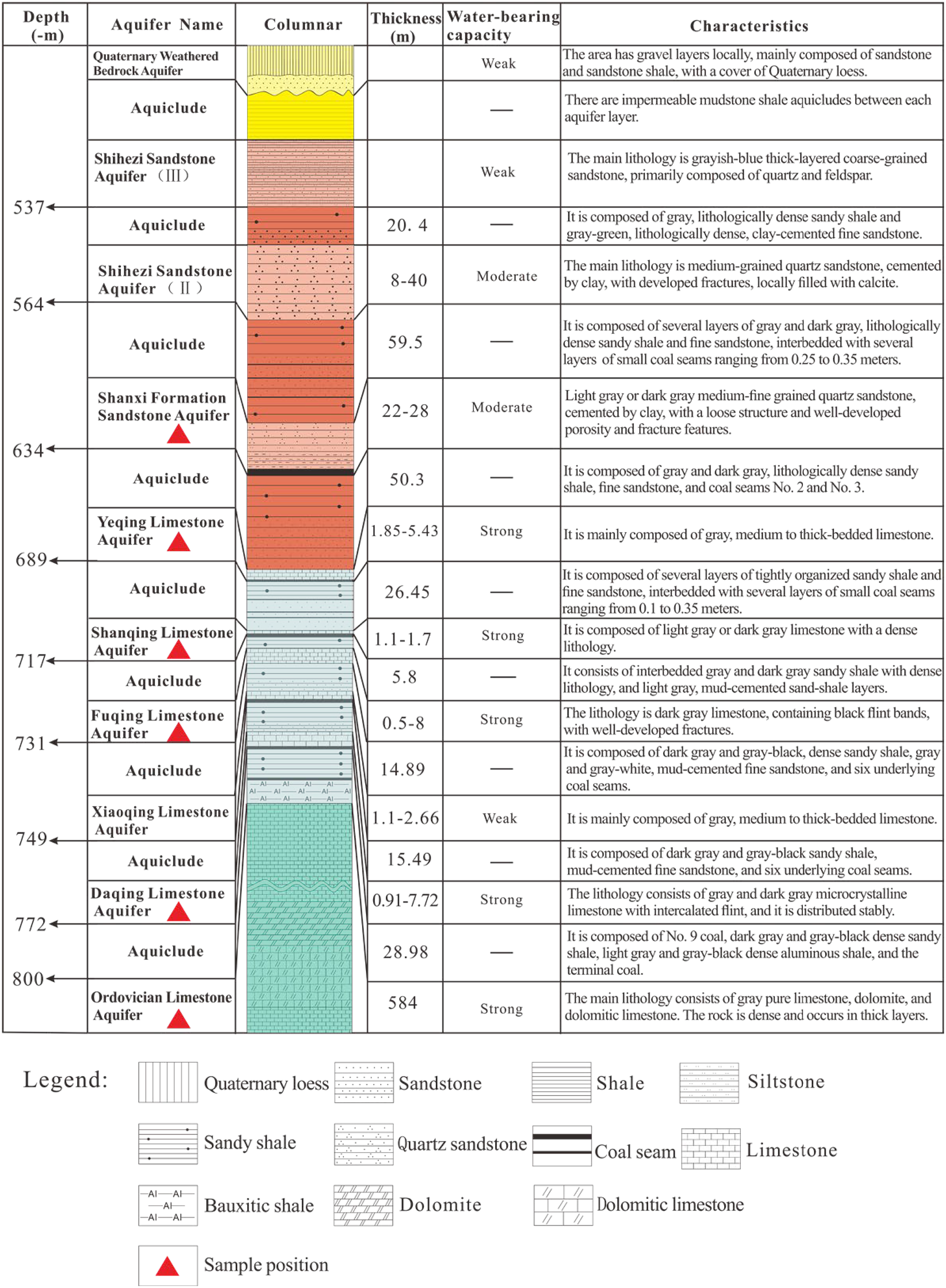
Comprehensive histogram of strata in the study area.

Materials and methods

Sampling and test methods

The distribution of water sampling points is presented in Figure 1. Some sampling locations overlap due to their close proximity. All polyethylene bottles were triple-rinsed with source water at each sampling point. Water samples were collected in bottles filled to capacity (no headspace) and immediately sealed with caps, and labeled on-site. No preservatives were added, with samples being stored at 4 °C and transported to the laboratory within 24 hours for conventional component analysis. Due to hydrogeological constraints in field sampling, the number of collected samples was insufficient for systematic characterization of major water-inrush aquifers in Sunzhuang Minefield. Therefore, supplementary hydrogeochemical data from the past decade were obtained from the mine operator. To ensure data validity, ionic balance verification was performed for each sample (equation (1)), where E represents the charge balance error (%); m_c and m_a the molar concentrations of cations and anions (mol/L), respectively; and Z the ionic charge number. Samples with a charge balance error exceeding the range of ±5% were discarded.

E = \frac{\sum Z \cdot m_{c} - \sum Z \cdot m_{a}}{\sum Z \cdot m_{c} + \sum Z \cdot m_{a}} \times 100 %

(1)

After eliminating disqualified data, a total of 86 groundwater samples were retained for analysis. This dataset included 16 samples from the Permian sandstone fractured aquifers (DS), 13 from Yeqing limestone aquifer (YQ), 16 from Shanfuqing limestone aquifer (SF), 20 from Daqing limestone aquifer (DQ), 15 from Ordovician limestone karst aquifers (AH), and 6 from water-inrush samples. Discrimination indicators included six major ions (Ca²⁺, Mg²⁺, K⁺ + Na⁺, HCO₃⁻, SO₄²⁻, Cl⁻) and three physicochemical parameters: electrical conductivity (EC), total dissolved solids (TDS), and total hardness (TH).

Entropy weight: Variable fuzzy set theory

Weight determination

Weight determination is crucial for calculating comprehensive relative membership degrees, as appropriate weight allocation directly impacts the accuracy of identification results. To achieve this objectively, we employed the Entropy Weight Method (EWM). In this context, entropy is a measure of the data dispersion for a given indicator. Its value reflects the amount of useful information that indicator provides. The core principle is that the greater the variability of an indicator's data across samples, the more valuable it is for classification. Specifically, an indicator with a small entropy value exhibits high data variation, making it highly effective for distinguishing between samples, and it is thus assigned a high weight. Conversely, an indicator with a large entropy value has more uniform data, offers less discriminatory power, and is therefore assigned a low weight. By determining weights based on the inherent variability of the data itself, the EWM provides a robust and objective foundation for our multi-indicator evaluation. The weight calculation procedure is as follows:

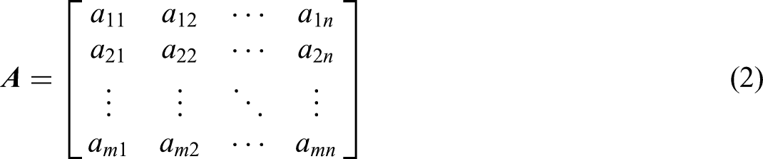
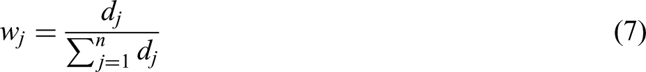
Construct the mean matrix A = (a_ij)_m _× _n. Based on actual measurement data, establish a normalized table with m rows representing evaluation objects and n columns representing evaluation indicators. For m evaluation objects classified into k categories, each element a_ij in matrix A represents the mean value of corresponding evaluation objects (i = 1, 2, …, m; j = 1, 2, …, n).

A = [\begin{matrix} a_{11} & a_{12} & \dots & a_{1 n} \\ a_{21} & a_{22} & \dots & a_{2 n} \\ ⋮ & ⋮ & ⋱ & ⋮ \\ a_{m 1} & a_{m 2} & \dots & a_{m n} \end{matrix}]

(2)

Data standardization: The range method was applied to normalize the measured data, eliminating dimensional and scale differences among variables. The standardized values for n indicators (x₁_j, x₂_j, …, x_m_j) are denoted as z_i_j, as expressed in equation (3):

z_{i j} = \frac{a_{i j} - min (a_{1 j}, a_{2 j}, a_{m j})}{max (a_{1 j}, a_{2 j}, a_{m j}) - min (a_{1 j}, a_{2 j}, a_{m j})}

(3)

Probability matrix calculation: For the j-th indicator of the i-th sample, probability normalization was performed with non-negative translation to determine proportion weights, as shown in equation (4):

p_{i j} = \frac{z_{i j} + 0.01}{\sum_{i = 1}^{m} (z_{i j} + 0.01)}

(4)

The entropy value calculation formula for evaluation indicators is given by equation (5):

e_{j} = - \frac{1}{\ln m} \sum_{i = 1}^{m} p_{i j} \ln (p_{i j}) (j = 1, 2, \dots, n)

(5)

Determination of evaluation indicator weights. The entropy weight w_j for each indicator essentially represents the proportional information utility value d_j among different indicators within the same sample, where a higher d_j value corresponds to a greater weight. The calculation formulas are given by equations (6) and (7):

d_{j} = 1 - e_{j}

(6)

w_{j} = \frac{d_{j}}{\sum_{j = 1}^{n} d_{j}}

(7)

Relative membership degree

Let A be a fuzzy concept set on the universe of discourse U. Fuzzy sets are mathematical constructs designed to represent vague conceptual categories, where u denotes any element in $U (u \in U)$ . The universe of discourse U is mathematically conceptualized as a continuous membership axis. The relative membership degree of any point u to the attractive property of fuzzy set A is denoted as µ_A(u), while its relative membership degree to the repulsive property of A is expressed as µ_A^c(u), as shown in equation (8).

D_{A} (\begin{matrix} u) \end{matrix} = μ_{A} (\begin{matrix} u) \end{matrix} - μ_{A}^{c} (\begin{matrix} u) \end{matrix}

(8)

D_A(u) is the represents the relative difference degree of u to fuzzy set A, µ_A(u) ∈[0,1], µ_A^c(u) ∈[0,1], and µ_A(u) + µ_A^c(u) = 1. When defining the relative difference degree of u to A as a mapping,

D_A:D→[−1,1], u|→D_A(u) ∈[−1,1], the relative membership degree µ_A(u) can be derived by equations (9) to (11).

μ_{A}^{c} (u) = 1 - μ_{A} (u)

(9)

D_{A} (u) = μ_{A} (u) - [1 - μ_{A} (u)] = 2 μ_{A} (u) - 1

(10)

μ_{A} (u) = [1 + D_{A} (u)] / 2

(11)

Determining the relative difference degree D_A(u) becomes pivotal for computing the relative membership degrees.

Relative difference degree

According to the definition of variable fuzzy sets, let X₀ = [a,b] be the attractive domain on the axis where the relative difference degree satisfies 0 < D_A(u) ≤ 1. Let X = [c,d] be an extended interval containing X₀ (X₀⊂X), where subintervals [c,a] and [b,d] represent the repulsive domain with −1 ≤ D_A(u) < 0. Point M within [a,b], typically the midpoint of the interval, satisfies D_A(u) = 1. The positional relationships among M, [a,b] and [c,d] are illustrated in Figure 3.

Figure 3.

The positional relationships among M, [a,b] and [c,d].

Let any value x within the interval X, when x lies to the left of point M, the relative difference function model is given by equation (12):

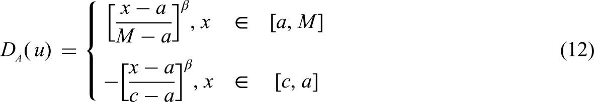
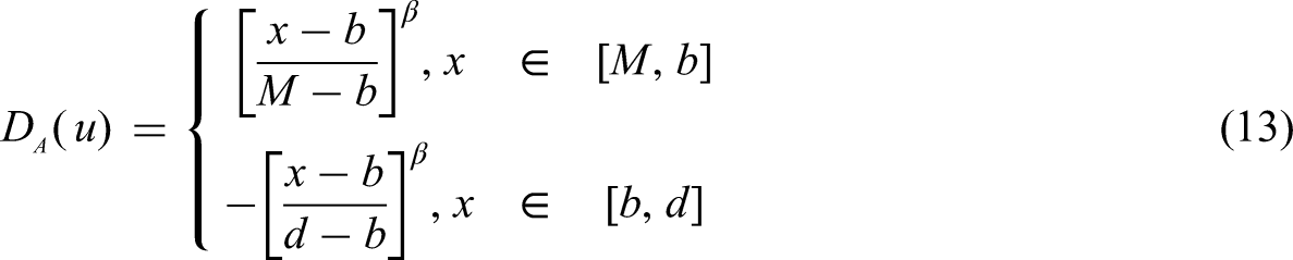
D_{_{A}} (\begin{matrix} u) \end{matrix} = {\begin{matrix} {[\frac{x - a}{M - a}]}^{β}, x & \in & [a, M] \\ - {[\frac{x - a}{c - a}]}^{β}, x & \in & [c, a] \end{matrix}

(12)

When x lies to the right of point M, the relative difference function model is given by equation (13):

D_{_{A}} (\begin{matrix} u) \end{matrix} = {\begin{matrix} {[\frac{x - b}{M - b}]}^{β}, x & \in & [M, b] \\ - {[\frac{x - b}{d - b}]}^{β}, x & \in & [b, d] \end{matrix}

(13)

When $x \notin [c, d]$ , the relative difference degree is calculated as D_A(u) = −1. β is a positive exponent typically set to 1. Equations (12) to (13) must satisfy three conditions: (1)when x = a or x = b, D_A(u) = 0; (2) when x = M, D_A(u) = 1; (3) when x = c or x = d, D_A(u) = −1. The relative membership degree μ_A(u) to be determined via equations (11).

Comprehensive relative membership degree

For the s-th sample to be identified, let u_s_h represent its comprehensive relative membership degree with respect to rank variable h, the weight w_j of the j-th indicator is determined by the entropy weight method and μ_A(jh) denotes the relative membership degree of indicator j to rank variable h. The comprehensive relative membership degree u_s_h can then be calculated using the variable fuzzy set recognition model, as shown in equation (14):

μ_{s h} = \frac{1}{1 + {(\frac{d_{h g}}{d_{h b}})}^{α}}

(14)

d_{h g} = {\sum_{j = 1}^{n} {[w_{j} (1 - μ_{A} (j h))]}^{p}}^{\frac{1}{p}}

(15)

d_{h b} = [\sum_{j = 1}^{n} (w_{j} μ_{A} (j h))^{p}]^{\frac{1}{p}}

(16)

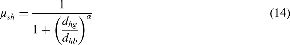
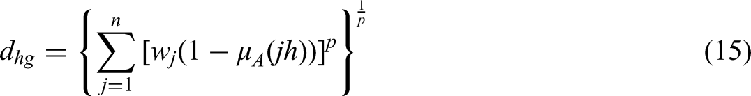
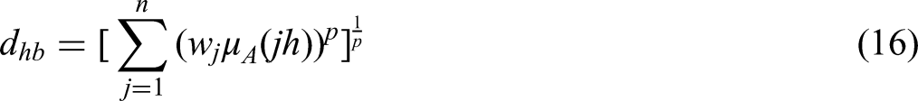
In equations (14)–(16), a denotes the optimization criterion parameter (with a = 1 for least absolute deviations and a = 2 for least squares), n the number of indicators; p the distance parameter (where p = 1 indicates Hamming distance and p = 2 Euclidean distance); d_hg the dissimilarity between sample s and water source h, while d_hb denotes their similarity.

Rank feature value

To transform fuzzy membership degrees into continuous quantitative indices, we define the sample's rank feature value H_i, as equation (17):

H_{i} = \sum_{h = 1}^{c} μ {^{'}}_{s h} h

(17)

where µ′_sh represents the normalized value of µ_sh and c the number of classification levels.

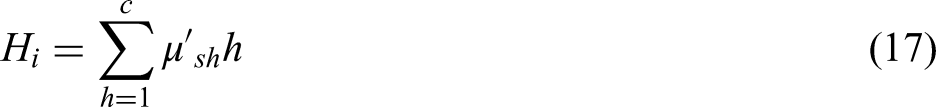
The H_i comprehensively integrates all information regarding the h and the μ_s_h, thereby enabling a more holistic and objective determination of the classification level for sample s. Consequently, H_i serves as an effective predictor of the membership relationship of sample s. Moreover, H_i is a numerical descriptor of fuzzy conceptual levels, typically noninteger valued and bounded by 0 ≤ H_i ≤ i. Geometrically, within the h-μ_s_h coordinate plane, H_i corresponds to the centroid position of the figure formed by the h and µ_sh. Therefore, this study employs H_i for predictive classification, rather than relying solely on the maximum membership principle for direct level assignment (Chen and Guo, 2005).

Integer distance evaluation

In water source discrimination, the ideal rank feature value H_i for sample s_i should closely approximate the aquifer category. H_i should approach integer values (e.g. 1, 2, 3,…) to clearly indicate which class the sample belongs to. The distance between each sample's H_i value and its nearest integer category is calculated under different parameters, with smaller distances indicating more accurate classification results. The absolute difference between H_i and their nearest integers under varying parameters is computed as shown in equation (18):

D_{i} = | H_{i} - r o u n d (H_{i}) |

(18)

round (H_i): the rounded integer value representing the theoretically ideal category.

The mean value $\bar{D}$ of all sample distances D_i under different parameter set is computed as shown in equation (19).

\bar{D} = \frac{1}{n} \sum_{i = 1}^{n} D_{i}

(19)

A smaller $\bar{D}$ indicates that H_i values are closer to integer categories, demonstrating clearer classification results. The parameter set corresponding to $\bar{D} = Min {{\bar{D}}_{1}, {\bar{D}}_{2}, {\bar{D}}_{3}, \dots, {\bar{D}}_{i}}$ is selected as the optimal parameter combination.

To provide a clear overview of the entire process, the computational procedure of the EW-VFS model is visualized in the schematic flowchart in Figure 4.

Figure 4.

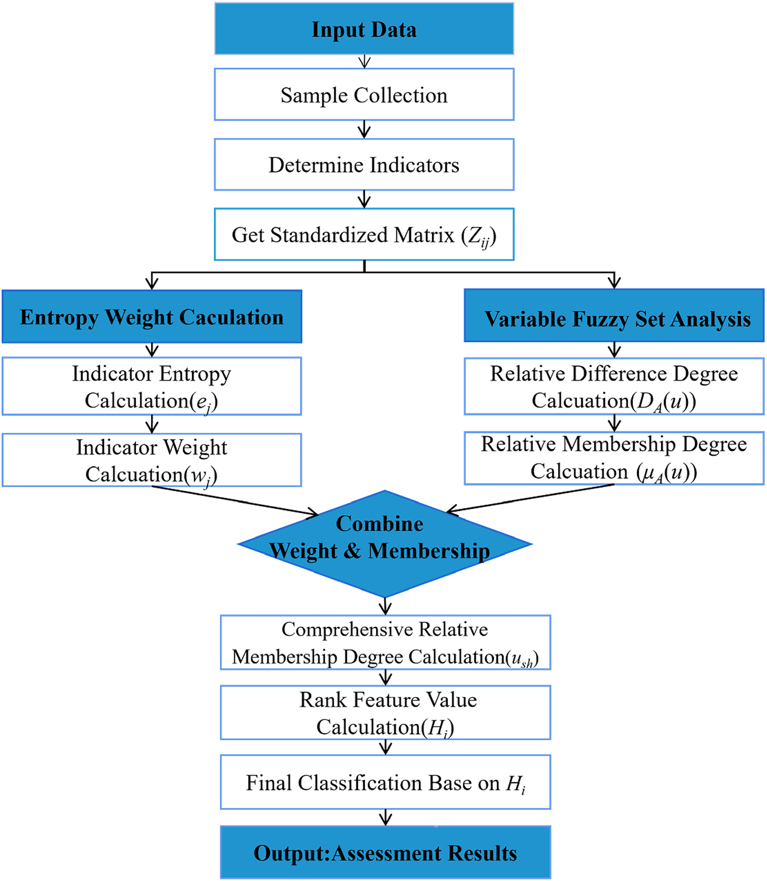
Schematic flowchart of the EW-VFS model steps.

Result and discussion

Descriptive statistical analysis of indicator

A statistical analysis was performed on conventional hydrogeochemical components and physicochemical parameters from 80 groundwater samples collected in the Sunzhuang Minefield, with the original mass concentrations of each indicator presented as box plots (Figure 5). In box plots, the left and right boundaries of the rectangular boxes correspond to the 25th (Q1) and 75th percentiles (Q3), respectively (Qian et al., 2018), while the central line represents the median. Square markers indicate mean values, and the whiskers extend to the minimum and maximum concentrations, with data points outside this range classified as outliers. Figure 5 can clearly demonstrate the distribution patterns of each parameter across the five aquifers and distinct variations of the same parameter among different aquifer types.

Figure 5.

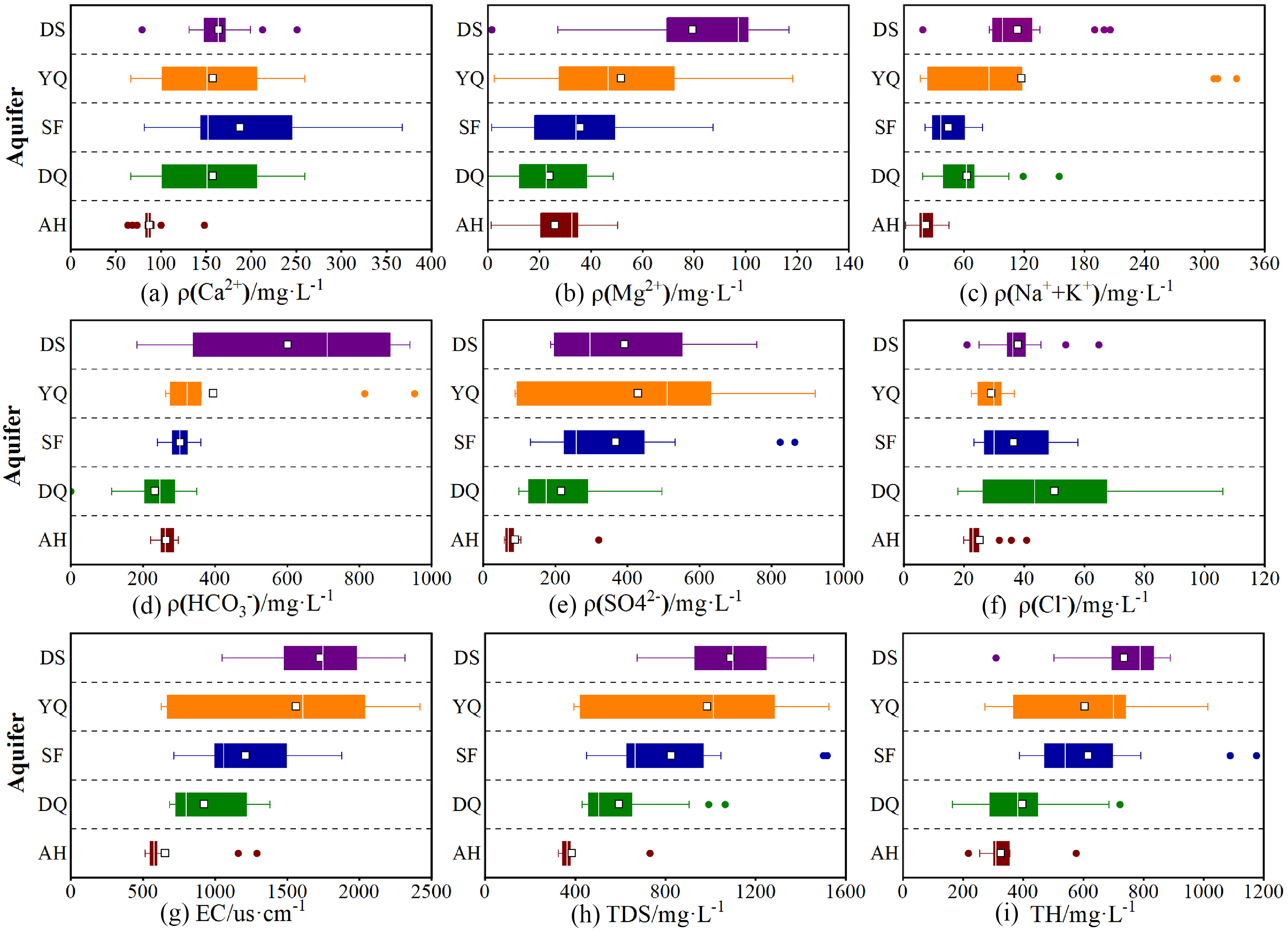
Box plots of conventional components and physicochemical parameters.

As evidenced by box plots B and D, the DS aquifer exhibits the highest mean concentrations of Mg²⁺ and HCO₃⁻, which serve as effective discriminators to distinguish it from other aquifers. The YQ aquifer shows higher SO₄²⁻ concentrations, while the SF aquifer contains the maximum Ca²⁺ levels. The DQ aquifer is characterized by elevated Cl⁻ concentrations coupled with depressed HCO₃⁻ levels, whereas the AH aquifer displays the lowest concentrations of Ca²⁺, Na⁺ + K⁺, SO₄²⁻, and Cl⁻ among all aquifers. These hydrogeochemical characteristics of the five aquifers are intrinsically linked to their host rock lithologies. The three physicochemical parameters (EC, TDS, and TH) exhibit a decreasing trend with increasing aquifer depth. Although parameter variations exist across aquifers, their values consistently cluster within specific ranges, showing higher probabilities near median values. This distribution pattern aligns with variable fuzzy set theory, where proximity to characteristic values enhances attraction (identification capability), whereas deviation increases repulsion (reduces identifiability). To enhance data robustness, the interquartile range (25%–75%) was adopted for analysis, with identified outliers being excluded.

Table 1 presents the statistical results after outlier removal for each aquifer. The data reveal that all aquifers in the study area exhibit high water hardness, classified as very hard water (TH > 180 mg/L). While the DS aquifer shows brackish characteristics (1000 mg/L < TDS < 3000 mg/L), the remaining aquifers maintain average TDS concentrations below 1000 mg/L, qualifying as freshwater. The coefficient of variation (CV), which quantifies data dispersion, exceeds 30% for HCO₃⁻ and SO₄²⁻ in the DS aquifer, Mg²⁺, Na⁺ + K⁺ and SO₄²⁻ in the YQ aquifer, Ca²⁺ and SO₄²⁻ in the SF aquifer, and Mg²⁺ in the DQ aquifer, indicating relatively high data variability. Other parameters across aquifers demonstrate lower CV values (<30%), reflecting more concentrated distributions within specific ranges (Zhang et al., 2020a).

Table 1.

Statistical results of aquifer parameters after outlier removal.

Variables		Ca²⁺	Mg²⁺	Na⁺+K⁺	HCO₃⁻	SO₄²⁻	Cl⁻	EC	TDS	TH
DS (N = 16)	Min	146.59	75.19	87.90	332.36	195.83	35.27	1050.00	676.85	503.43
	Max	172.00	117.00	119.60	941.00	577.92	38.99	2317.46	1460.00	890.46
	Mean	161.29	98.03	99.30	684.84	381.85	36.50	1710.20	1078.28	732.92
	CV(%)	5.65	13.06	10.77	35.89*	42.31*	3.08	20.19	20.02	16.06
YQ (N = 13)	Min	101.55	27.81	23.59	274.13	88.93	24.70	628.82	396.16	274.15
	Max	206.42	72.30	118.22	361.91	632.00	32.40	2423.52	1526.82	1014.53
	Mean	159.22	46.89	74.14	317.88	325.84	28.77	1564.47	985.62	606.27
	CV(%)	29.53	33.33*	45.89*	11.57	69.10*	10.89	44.99	44.99	40.29
SF (N = 16)	Min	127.84	27.20	28.91	241.24	131.97	26.70	715.92	451.03	388.40
	Max	348.51	45.32	60.75	323.47	533.00	46.99	1882.00	1251.35	924.88
	Mean	186.34	35.40	43.44	294.82	299.85	33.60	1211.95	795.09	591.38
	CV(%)	35.77*	19.05	28.52	7.97	39.16*	25.38	25.98	30.28	29.58
DQ (N = 20)	Min	91.39	13.33	43.49	212.00	122.66	28.33	685.57	431.91	165.28
	Max	123.00	38.54	67.81	280.66	268.64	67.60	1382.00	892.36	677.96
	Mean	110.45	25.68	58.97	251.32	174.62	47.88	926.09	580.75	395.92
	CV(%)	10.19	31.47*	15.76	8.57	24.66	28.54	27.00	28.41	34.97
AH (N = 15)	Min	83.01	20.60	15.81	250.77	59.27	21.84	518.27	326.51	248.07
	Max	88.30	35.00	28.55	285.47	84.80	24.99	622.44	425.27	356.00
	Mean	86.04	28.94	19.70	264.42	71.36	23.40	575.96	365.73	314.00
	CV(%)	1.96	22.49	21.15	4.72	12.61	4.43	5.75	7.18	11.38

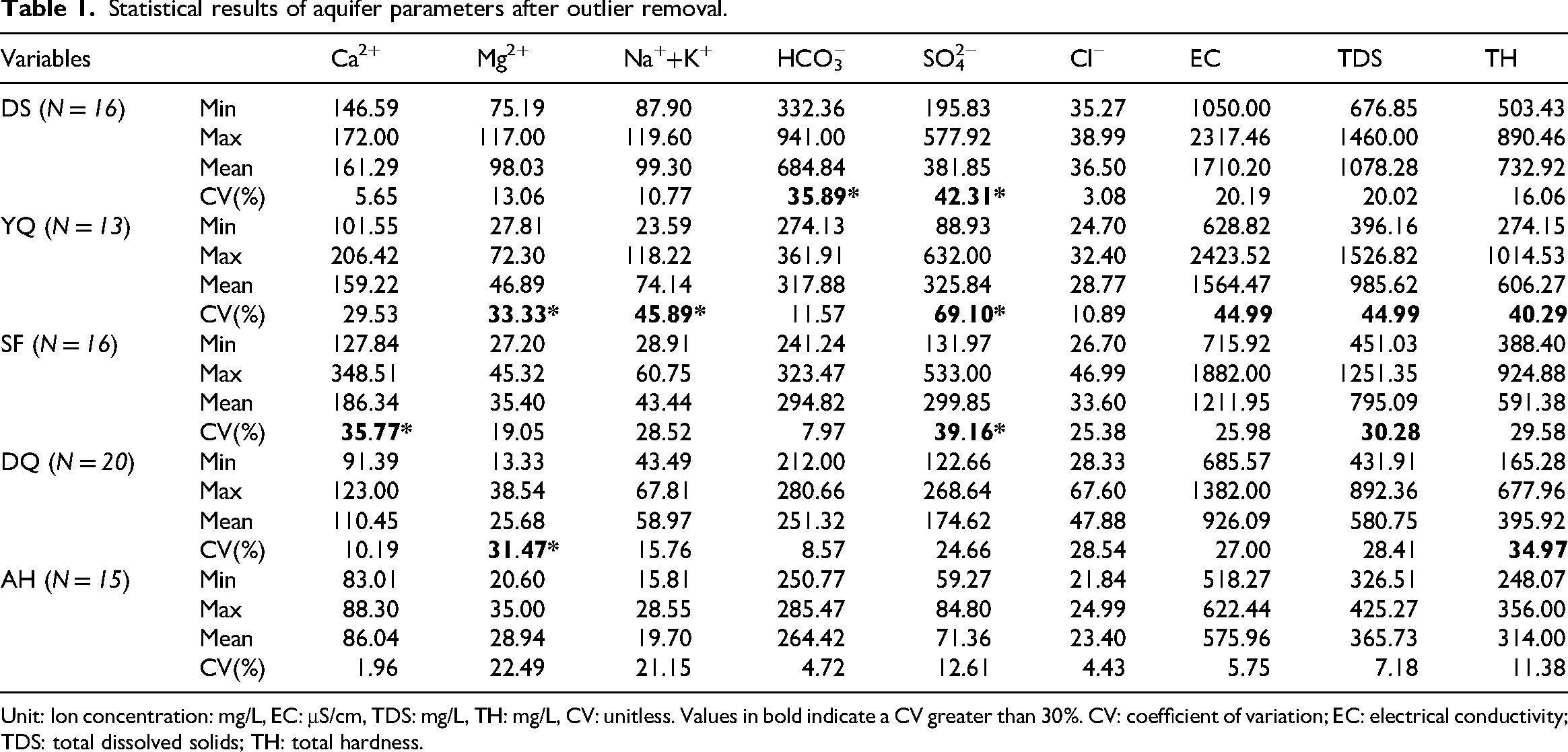
Unit: Ion concentration: mg/L, EC: μS/cm, TDS: mg/L, TH: mg/L, CV: unitless. Values in bold indicate a CV greater than 30%. CV: coefficient of variation; EC: electrical conductivity; TDS: total dissolved solids; TH: total hardness.

Outliers in hydrogeochemical indicators for each aquifer were determined using box plot analysis, with subsequent data processing conducted, six conventional ions were selected to form the basis for developing the water source identification model. Since EC, TDS, and TH are linear combinations of these conventional ions (Hussain et al., 2019), to prevent data redundancy and maintain model discriminative performance, these parameters were retained solely for statistical characterization.

Development of discrimination model

In this study, we established identification intervals using 80 water samples from 5 types of aquifers as the training set. For this set, the influence of outlier values within each indicator was addressed by using the mean-standard deviation classification method (Wang et al., 2017) to determine threshold parameters: [a, b] = [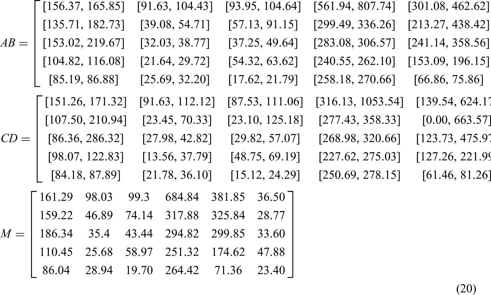 $\bar{x}$ −0.5σ, $\bar{x}$ + 0.5σ] and [c, d] = [ $\bar{x}$ −1.1σ, $\bar{x}$ + 1.1σ]. For indicators with CV > 30% in Table 1, the rejection boundaries [c, d] were expanded to [ $\bar{x}$ −1.5σ, $\bar{x}$ + 1.5σ]. When c < 0, it was set to 0. Three matrices were derived: matrix AB ([a, b]), matrix CD ([c, d]), and matrix M ( $\bar{x}$ ). Subsequently, the established EW-VFS model was validated using a test set of 6 representative water samples from a mine inrush event.

\begin{aligned} A B = [\begin{matrix} [156.37, 165.85] & [91.63, 104.43] & [93.95, 104.64] & [561.94, 807.74] & [301.08, 462.62] & [35.93, 37.06] \\ [135.71, 182.73] & [39.08, 54.71] & [57.13, 91.15] & [299.49, 336.26] & [213.27, 438.42] & [27.20, 30.34] \\ [153.02, 219.67] & [32.03, 38.77] & [37.25, 49.64] & [283.08, 306.57] & [241.14, 358.56] & [29.33, 37.86] \\ [104.82, 116.08] & [21.64, 29.72] & [54.32, 63.62] & [240.55, 262.10] & [153.09, 196.15] & [41.04, 54.71] \\ [85.19, 86.88] & [25.69, 32.20] & [17.62, 21.79] & [258.18, 270.66] & [66.86, 75.86] & [22.88, 23.92] \end{matrix}] \\ C D = [\begin{matrix} [151.26, 171.32] & [91.63, 112.12] & [87.53, 111.06] & [316.13, 1053.54] & [139.54, 624.17] & [35.26, 37.73] \\ [107.50, 210.94] & [23.45, 70.33] & [23.10, 125.18] & [277.43, 358.33] & [0.00, 663.57] & [25.32, 32.21] \\ [86.36, 286.32] & [27.98, 42.82] & [29.82, 57.07] & [268.98, 320.66] & [123.73, 475.97] & [24.22, 42.97] \\ [98.07, 122.83] & [13.56, 37.79] & [48.75, 69.19] & [227.62, 275.03] & [127.26, 221.99] & [32.84, 62.91] \\ [84.18, 87.89] & [21.78, 36.10] & [15.12, 24.29] & [250.69, 278.15] & [61.46, 81.26] & [22.26, 24.54] \end{matrix}] \\ M = [\begin{matrix} 161.29 & 98.03 & 99.3 & 684.84 & 381.85 & 36.50 \\ 159.22 & 46.89 & 74.14 & 317.88 & 325.84 & 28.77 \\ 186.34 & 35.4 & 43.44 & 294.82 & 299.85 & 33.60 \\ 110.45 & 25.68 & 58.97 & 251.32 & 174.62 & 47.88 \\ 86.04 & 28.94 & 19.70 & 264.42 & 71.36 & 23.40 \end{matrix}] \end{aligned}

(20)

Based on the positional relationships among matrices AB, CD, and M, equations (12) to (13) were applied to calculate their relative difference degrees, while equation (10) was used to determine the relative membership degrees.

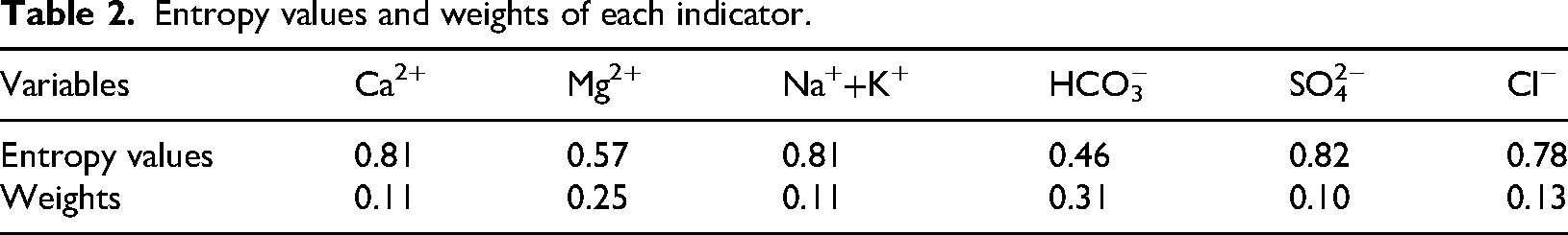
We calculated the entropy values and corresponding weights of each hydrogeochemical indicator using the entropy weight method (equations (5) and (6)), with results summarized in Table 2. The analysis revealed that Mg²⁺ and HCO₃⁻ carried significantly higher weights of 0.2467 and 0.3079, respectively, compared to other indicators. Collectively, these two ions accounted for 55.46% of the total weighting, demonstrating their more dispersed distributions across the five aquifer types and highlighting their particular importance in discriminating water-inrush sources among different aquifers.

Table 2.

Entropy values and weights of each indicator.

Variables	Ca²⁺	Mg²⁺	Na⁺+K⁺	HCO₃⁻	SO₄²⁻	Cl⁻
Entropy values	0.81	0.57	0.81	0.46	0.82	0.78
Weights	0.11	0.25	0.11	0.31	0.10	0.13

Following the calculation of relative membership degrees µ_A(u) and weight values w_j, the comprehensive relative membership degree µ_sh and rank feature value H_i were determined using equation (14) and (17). The water source type was identified by optimizing the model through maximum membership degree and rank feature value analysis.

Water inrush source identification

The 12661 working face in Sunzhuang Coal Mine is the first mining panel of the No. 6 coal seam, located at a depth of 500 m below surface. Understanding its hydrogeological conditions during mining provides critical guidance for subsequent mining under pressure safe production. The SF limestone aquifer is the immediate roof of the working face, predominantly manifested roof water dripping and floor water seepage during extraction operations. When encountering structural fractured zones, the water inflow transient increased, causing measurable impacts on mining productivity. The DQ is confined aquifer in the floor, featuring developed karst fissures and hydraulic connectivity with the AH aquifer, demonstrated high water abundance. Its water-inrush coefficient of 0.06 MPa/m (Li et al., 2024) exceeded the critical threshold, indicating significant outburst risks. Prior to mining, surface-based regional groundwater grouting control was conducted on the DQ aquifer of working face 12661, with systematic slurry injection into fissure networks. Post-treatment verification confirmed the successful transformation of the DQ aquifer into a weakly permeable aquifer or relatively impermeable layer, significantly enhancing the floor aquiclude's water-resisting and pressure-bearing capacity. Investigation confirmed the working face is unaffected by atmospheric precipitation, goaf water, and fault water.

Water-inrush incidents occurred during formal mining operations after regional groundwater grouting control. To discrimination the water sources, six water samples were collected sequentially at the water-inrush point for hydrogeochemical analysis. The established discrimination model was then applied to predict the source aquifers of these inrush samples, with the measure parameters and corresponding results detailed in Table 3.

Table 3.

Water-inrush source identification results.

No.	Source	Time	Hydrogeochemical composition/(mg·L⁻¹)						Actual type	Identifying type
No.	Source	Time	Ca²⁺	Mg²⁺	Na⁺+K⁺	HCO₃⁻	SO₄²⁻	Cl⁻	Actual type	Identifying type
1	12661 roadway	20210119	82.16	3.20	60.55	244.08	104.14	25.49	SF	DQ
2	12661 working face	20210319	103.00	4.37	81.17	45.76	146.12	123.46	SF	SF
3	12661 working face	20210319	2.23	4.65	159.33	192.22	139.94	30.49	SF	SF
4	12661 working face	20210324	113.43	7.70	95.46	234.93	251.90	30.49	SF	SF
5	12661 roadway	20210508	109.42	4.39	101.77	289.84	206.62	31.99	SF	SF
6	12661 working face	20210524	83.77	2.11	45.48	158.65	128.83	33.49	SF	SF

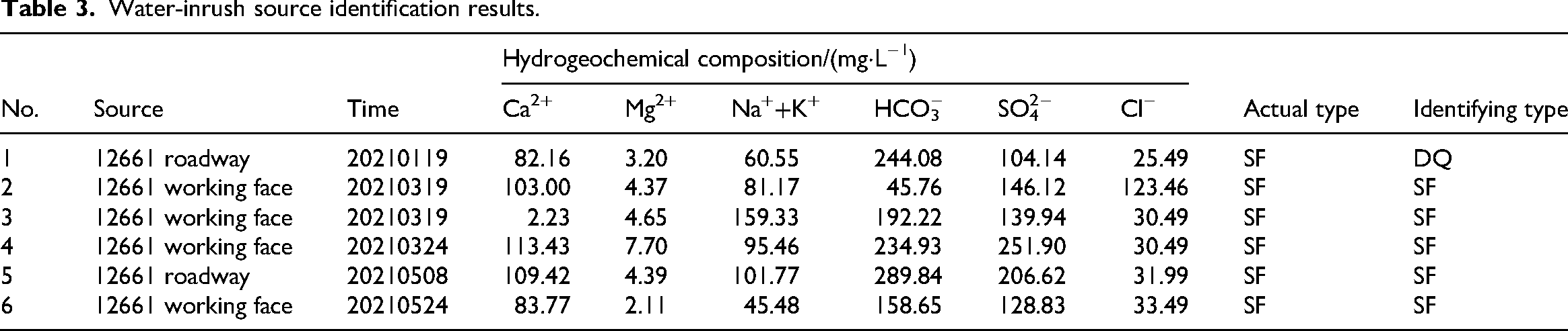
Taking water-inrush sample 1 s_1j = (82.16, 3.20, 60.55, 244.08, 104.14, 25.49) as an example, the first parameter s₁₁ (Ca²⁺ concentration) was compared with the corresponding Ca²⁺ values in matrices AB_1h, CD_1h, and M_1h from equation (20) to determine their relative positions. For instance: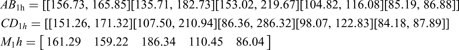

\begin{aligned} A B_{1 h} = [[156.73, 165.85] [135.71, 182.73] [153.02, 219.67] [104.82, 116.08] [85.19, 86.88]] \\ C D_{1 h} = [[151.26, 171.32] [107.50, 210.94] [86.36, 286.32] [98.07, 122.83] [84.18, 87.89]] \\ M_{1} h = [\begin{matrix} 161.29 & 159.22 & 186.34 & 110.45 & 86.04 \end{matrix}] \end{aligned}

Given s₁₁ = 82.16, a₁₁ = [156.73, 165.85], c₁₁ = [151.26, 171.32], and M₁₁ = 161.29, the condition s₁₁∉[c,d] therefore relative difference degree D_A(s₁₁) = −1. Subsequently, the relative membership degree µ_A(s₁₁) = 0 was calculated using equation (11). Similarly, the relative membership degrees of s₁₁ for other h-level intervals (representing different aquifers) were determined, forming the relative membership degree matrix U(s₁).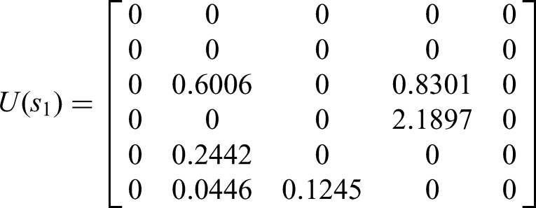

U (s_{1}) = [\begin{matrix} 0 & 0 & 0 & 0 & 0 \\ 0 & 0 & 0 & 0 & 0 \\ 0 & 0.6006 & 0 & 0.8301 & 0 \\ 0 & 0 & 0 & 2.1897 & 0 \\ 0 & 0.2442 & 0 & 0 & 0 \\ 0 & 0.0446 & 0.1245 & 0 & 0 \end{matrix}]

The comprehensive membership degree vector μ_1h for water-inrush sample s₁ was calculated using the weights from Table 2 and equation (14), with the optimization criterion parameter set as α=2 and distance parameter p = 1.

μ_{1 h} = [\begin{matrix} 0 & 0.0113 & 0.0003 & 0.9141 & 0 \end{matrix}]

After normalization, the results are as follows:

μ_{1 h}^{'} = [\begin{matrix} 0 & 0.0122 & 0.0003 & 0.9875 & 0 \end{matrix}]

The rank feature values (H_i) were calculated using equation (17) as follows:

H_{1} = 3.9753

According to the evaluation criterion for rank feature values (Chen and Han, 2006): if H ∈ [h−0.5, h + 0.5] (h = 1, 2, 3, 4, 5), the evaluated sample is classified as grade h. In this study, the water sources DS, YQ, SF, DQ, and AH correspond to grades 1, 2, 3, 4, and 5, respectively. Since H₁ = 3.9753 ∈ [3.5, 4.5], it is conclusively identified as grade 4 water (DQ water).

Analysis of results

Based on the above content, the sources of the other five water-inrush samples were successfully identified, with classification results presented in Table 4. The entropy-weighted fuzzy variable set model achieved an overall accuracy of 83.33%, correctly identifying five of the six test samples. This result demonstrates both the advancement and reliability of our model. Specifically, it surpasses the 75.86% accuracy achieved by traditional fuzzy methods in the same study area (Guo et al., 2017). Furthermore, it is consistent with the 87.5% accuracy reported for this method in other contexts (Wang et al., 2017). As evident from Table 4, the model demonstrates particularly strong performance in discriminating DS and AH aquifers.

Table 4.

Comprehensive relative membership degrees and rank feature values.

Samples No.	Comprehensive relative membership degree (µ_sh)					Rank feature value (H_i)
Samples No.	DS	YQ	SF	DQ	AH	Rank feature value (H_i)
1	0	0.0113	0.0003	0.9141	0	3.9753
2	0	0.0190	0.0006	0.0068	0	2.5348
3	0	0.0101	0.0091	0.0007	0	2.5258
4	0.0139	0.0497	0.0364	0.0377	0	2.7112
5	0.0138	0.0492	0.3075	0.0208	0	2.8570
6	0	0.0052	0.0728	0.0001	0	2.9349

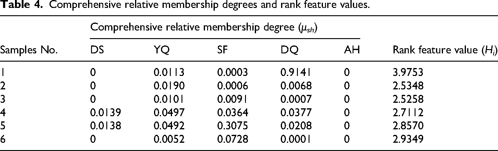
Figure 6 plots the data from Table 4 as a line chart, using the H_i values of six water samples to quantify the dynamic transition of the inrush source. This transition shows a shift from water predominantly from the DQ aquifer to water dominated by the SF aquifer due to mining disturbances. Figure 7 presents the conceptual model illustrating this mining-induced water source evolution. As shown in Figure 7(a) illustrating the postgrouting and premining stage. Surface-based regional groundwater grouting control was conducted in the mining area, including sealing of primary fractures and other water-conducting pathways, as well as reinforcement and thickening of the aquiclude, to reduce the risk of water inrush from the DQ confined aquifer into the working face. Figure 7(b) illustrating mixed inflow stage dominated by DQ aquifer. Mining-induced disturbances have generated secondary fractures in the roof and floor strata, which establish hydraulic connections with aquifers. Despite prior regional groundwater grouting control, localized residual inflows of DQ confined water may still reach the working face. This initial stage, water sample 1 (H_i = 3.9753) indicates absolute dominance of DQ water in the inrush source. Figure 7(c) illustrating the SF aquifer groundwater becomes the dominant water-inrush source. With time the pressure and flow rate of the DQ confined aquifer gradually decrease. Water samples 2 and 3, collected subsequently at the same time point, exhibit H_i values of 2.5348 and 2.5258, respectively. This marks the beginning of a transitional phase in the inrush source composition from DQ to SF water. Subsequent samples 4 to 6 demonstrate a continued trend with H_i values rising from 2.7112 to 2.9349, ultimately confirming SF water as the primary inrush source under mining-induced stress conditions.

Figure 6.

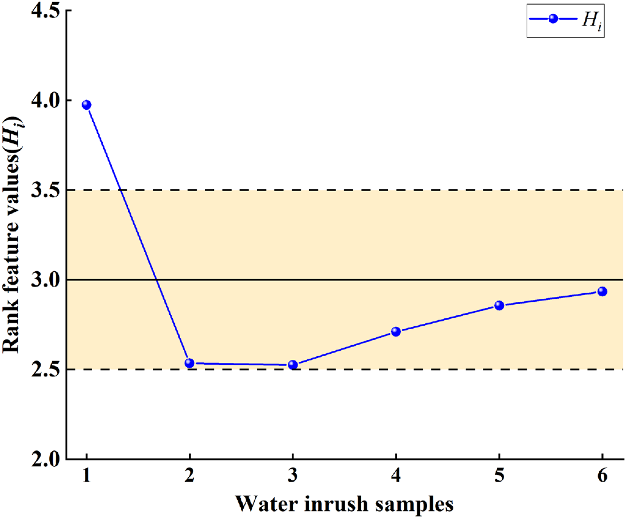
Variation curve of rank feature values (H_i).

Figure 7.

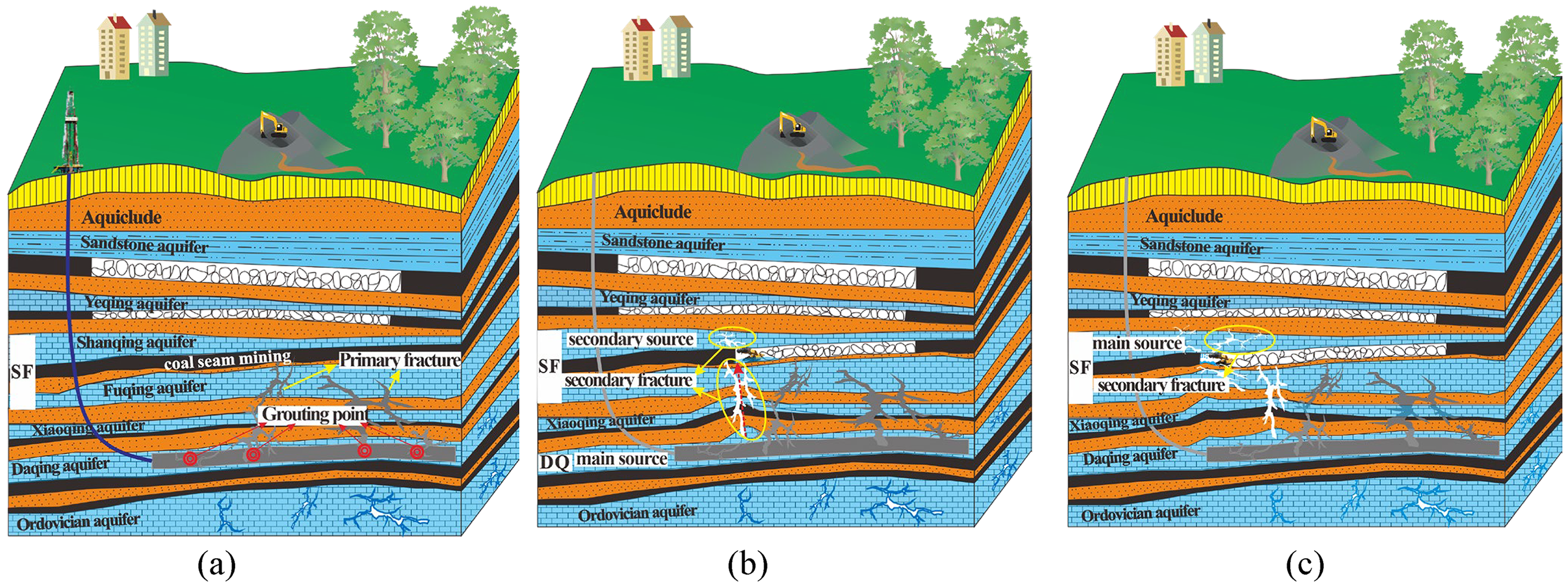
Model diagram of water-inrush process induced by mining. (a) postgrouting and premining preparation; (b) mixed inflow stage dominated by the DQ aquifer; and (c) the SF aquifer groundwater becoming the dominant source.

The misclassification of sample 1 as DQ water primarily stems from two factors: On the one hand, the limited number of reference samples for SF and DQ water led to imprecise discriminant intervals during model construction. For instance, the characteristic interval of threshold parameters [c, d] for Ca²⁺ in DQ water [98.07, 122.83] was found to be entirely contained within the broader range for SF water [86.36, 286.32]. This interval overlap meant that the model could not uniquely distinguish the two sources based on this key ion, contributing directly to the classification error. On the other hand, hydrogeological analysis revealed that both SF and DQ waters originate from adjacent thin limestone aquifers within the Carboniferous Taiyuan Formation. Combined effects of coal seam mining and confined aquifer pressure promoted the development of water-conducting fracture zones in surrounding rocks. Initial stage, the DQ water preferentially intruded into the working face through these dominant flow pathways, establishing it as the primary water source. Since premining regional floor grouting control effectively transformed the DQ aquifer into a weakly permeable zone. The residual water pressure was rapidly released and progressively diminished over time. Concurrently, SF water as the immediate roof and floor aquifer gradually assumed dominance through developing fracture networks, driving the hydrogeochemical transition from initial DQ water predominance to eventual SF water dominance in subsequent samples.

While the entropy-weighted variable fuzzy set model demonstrated superior performance in distinguishing DS and AH waters, further improvements are needed for accurate identification of thin limestone aquifers.

Table 5 presents the identification results of the entropy-weighted variable fuzzy set model based on equations (14) and (17) under different parameter configurations.

Table 5.

Identification results of the fuzzy variable set model under different parameters.

Samples No.	α = 1, p = 1	α = 1, p = 2	α = 2, p = 1	α = 2, p = 2	$\bar{H}$
1	3.7618*	3.5867*	3.9753*	3.9238*	3.8119
2	2.7758	2.7627	2.5348	2.5095	2.6457
3	2.6736	2.7990	2.5258	2.6735	2.6680
4	2.6242	2.6509	2.7112	2.8397	2.7065
5	2.3556*	2.6517	2.8570	2.8356	2.6750
6	2.7994	2.7767	2.9349	2.9130	2.8560

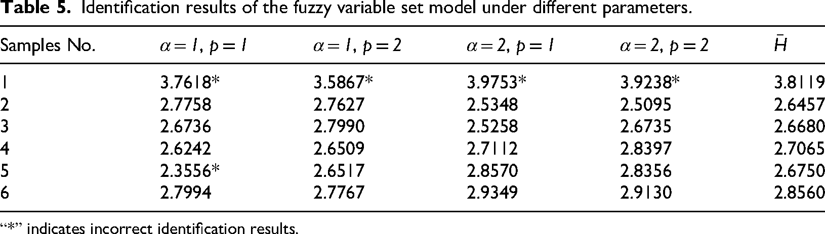
“*” indicates incorrect identification results.

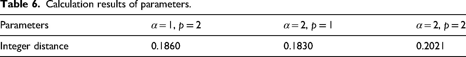
It is evident that the model yields significantly higher errors in identification when the optimization criterion parameter α = 1 and distance parameter p = 1. The other three parameter combinations produce relatively consistent discrimination results. Using integer distance evaluation for the remaining groups, the calculated H_i values demonstrate that the parameter set α = 2, p = 1 achieves the minimal deviation from the nearest integer class in Table 6. This indicates its classification results best align with theoretical expectations, thus being selected as the final model parameters.

Table 6.

Calculation results of parameters.

Parameters	α = 1, p = 2	α = 2, p = 1	α = 2, p = 2
Integer distance	0.1860	0.1830	0.2021

The water source identification model developed in this study established discrimination intervals for five aquifer types during water-inrush analysis. Boxplot (Figure 5) visualization revealed overlapping ranges for certain hydrogeochemical indicators. Water samples falling within these overlap zones may decrease identification accuracy due to ambiguous classification boundaries. Therefore, future water source discrimination methods require further optimization based on existing historical data. Firstly, the sampling number should be expanded, for instance, by implementing stratified monitoring programs. Secondly, time-series analysis should be incorporated to study the dynamic hydrogeochemical variations that occur during inrush events. The discrimination thresholds M, [a b], and [c d] should be determined based on comprehensive spatiotemporal water quality monitoring datasets to further enhance the accuracy of water source identification.

Conclusions

Through systematic analysis of hydrogeochemical data from 80 water samples in the Sunzhuang mine field, this study achieved refined classification of aquifers. The boxplot statistical method effectively delineated characteristic indicator ranges for five distinct aquifer types. This analysis established a reliable data foundation for constructing the entropy-weighted variable fuzzy set model. In particular, the discrimination capability of each indicator was determined through coefficient of variation analysis.

The model employed the entropy weight method for objective weighting, identifying Mg²⁺ and HCO₃⁻ as the most discriminative indicators with respective weights of 24.67% and 30.79%. Based on the entropy-weighted variable fuzzy set approach with dynamic membership functions and rank feature values quantification, it achieved 83.33% accuracy in water-inrush source identification. The model demonstrates effective discrimination between the DS and AH aquifers, but its accuracy in distinguishing thin limestone aquifers requires further improvement.

Temporal evolution analysis based on rank feature values (H_i) revealed a three-phase water-inrush pattern: (1) initial DQ water dominance (H_i = 3.98), (2) transitional mixing of DQ and SF waters (H_i≈2.5), and (3) stable SF water inflow regime (H_i = 2.71–2.93). This finding provides empirical evidence for understanding the evolutionary mechanisms of hydraulic connections among multiple aquifers under mining-induced disturbances.

Although the entropy-weighted variable fuzzy set model successfully achieved dynamic characterization of water source mixing patterns in this study area, the reliability and applicability of the model still heavily depend on the completeness of hydrogeological data. Therefore, it is critical to prioritize the collection and analysis of spatiotemporal water quality data from all major water-inrush aquifers to ensure accurate source identification.

Footnotes

Acknowledgements

We sincerely appreciate Sunzhuang Coal Mine for providing essential data support for this study.

ORCID iDs

Jian Liang

Wenwu Zhao

Shiming Liu

Yaoming Hang

Heyu Cui

Funding

The authors disclosed receipt of the following financial support for the research, authorship, and/or publication of this article: this work was supported by the Key Research and Development Program of Hebei Province (grant no. 22374204D).

Declaration of conflicting interests

The authors declared no potential conflicts of interest with respect to the research, authorship, and/or publication of this article.

Data availability

The datasets supporting the findings of this study are available from the corresponding author on reasonable request

References

Aris

Abdullah

Ahmed

, et al. (2007) Controlling factors of groundwater hydrochemistry in a small island’s aquifer. International Journal of Environmental Science & Technology 4: 441–450.

Belkhiri

Boudoukha

Mouni

, et al. (2010) Application of multivariate statistical methods and inverse geochemical modeling for characterization of groundwater—a case study: Ain azel plain (Algeria). Geoderma 159: 390–398.

Chen

Liu

, et al. (2022) Hydrochemical characteristics and source analysis of deep groundwater in qianyingzi coal mine. Coal Geology & Exploration 50: 99–106.

Chen

Gui

Yin

(2011) Monitoring of flow field based on stable isotope geochemical characteristics in deep groundwater. Environmental Monitoring and Assessment 179: 487–498.

Chen

Zhang

, et al. (2023) Progress of research on key technologies for hydrogeochemical prospecting in north China type coalfield. Coal Geology & Exploration 51: 207–219. (in Chinese).

Chen

Gui

(2021) Calculating groundwater mixing ratios in multi-aquifers based on statistical methods: A case study. Water Practice and Technology 16: 621–632.

Chen

(1993) On relative membership degree. Exploration of Nature 2: 25–27. (in Chinese).

Chen

(2005) Engineering variable fuzzy set theory and models: Mathematical foundations for fuzzy hydrology and water resources science. Journal of Dalian University of Technology 308: 312. (in Chinese).

Chen

Guo

(2005) Model of variable fuzzy sets and its application to classification prediction of Rockburst. In: Proceedings of the 9th National Conference on Rock Dynamics, pp.7–13. (in Chinese).

10.

Chen

Han

(2006) Engineering method of variable fuzzy set for assessment of surrounding rock stability. Chinese Journal of Rock Mechanics and Engineering 9: 1857–1861. (in Chinese).

11.

Guo

Wang

(2017) Determining source of water inrush of abandoned mine in Fengfeng mining area. Coal Technology 36: 162–164. (in Chinese).

12.

Hamed

Dassi

Tarki

(2011) Groundwater origins and mixing pattern in the multilayer aquifer system of the Gafsa-south mining district: A chemical and isotopic approach. Environmental Earth Sciences 63: 1355–1368.

13.

Hao

Zhang

Sun

, et al. (2021) Study on hydro-geochemistry processes of deep Ordovician limestone water of Fengfeng coal mining area. China Mining Magzaine 30: 230–236.

14.

Hou

Huang

Zhang

, et al. (2024) Identification of groundwater hydrogeochemistry and the hydraulic connections of aquifers in a complex coal mine. Journal of Hydrology 628: 130496.

15.

Huang

Wang

Han

(2017) Recognition model of groundwater inrush source of coal mine: A case study on jiaozuo coal mine in China. Arabian Journal of Geosciences 10: 323.

16.

Hussain

Wei

Luo

(2019) Hydrogeochemical characteristics, source identification and health risks of surface water and groundwater in mining and non-mining areas of Handan, China. Environmental Earth Sciences 78: 402.

17.

Kai

Hui

Guilei

, et al. (2023) Hydrogeochemical modeling of karst groundwater in the Fengfeng mining area. Water Resources 50: 948–959.

18.

, et al. (2024) Diffusion mechanism of variable-rate grouting in water prevention and control of coal mine. Water 16: 2814.

19.

Liu

Han

Fan

(2017) Discriminated method of mine water inrush source based on entropy weight fuzzy comprehensive analysis. Coal Mining Technology 22: 82–84, 9. (in Chinese).

20.

Qian

Tong

, et al. (2018) Hydrochemical characteristics and groundwater source identification of a multiple aquifer system in a coal mine. Mine Water and the Environment 37: 528–540.

21.

Liao

Wang

, et al. (2023) Hydrochemical evolution of groundwater in overburden aquifers under the influence of mining activity: Combining hydrochemistry and groundwater dynamics analysis. Environmental Earth Sciences 82: 135.

22.

Wang

Shi

, et al. (2018) Using stable isotopes (δD, δ18O, δ34S and 87Sr/86Sr) to identify sources of water in abandoned mines in the Fengfeng coal mining district, northern China. Hydrogeology Journal 26: 1443–1453.

23.

Sun

Bian

Wang

, et al. (2023) Hydrogeochemical characteristics and genetic analysis of karst groundwater in the Fengfeng mining area. Water 15: 4049.

24.

Sun

Hao

Huang

, et al. (2019) Drift characteristics of hydrogen and oxygen isotopes in Ordovician karst groundwater in Fengfeng mining area. China Mining Magazine 28: 151–157.

25.

Wang

Zhai

, et al. (2022) Temporal variation of hydrogeochemical characteristics and processes of aquifers in the Liuqiao coal mine. Energy Exploration & Exploitation 40: 1382–1393.

26.

Wang

Nie

, et al. (2019) Comprehensive prediction and discriminant model for Rockburst intensity based on improved variable fuzzy sets approach. Applied Sciences 9: 3173.

27.

Wang

Zhao

Wang

, et al. (2018) Determining the quality of mine gushing and mixed water using coupled AHP and fuzzy comprehensive evaluation methods. Scientific Research Publishing 10: 1185–1197.

28.

Wang

Yan

Guo

, et al. (2024) Vertical zoning characteristics and genesis mechanism of groundwater hydrochemistry: A case study of Xinjie mining area. Coal Science and Technology 52: 222–233. (in Chinese).

29.

Wang

Zhao

Liu

, et al. (2017) Identification of water inrush source from coalfield based on entropy weight-fuzzy variable set theory. Journal of China Coal Society 42: 2433–2439. (in Chinese).

30.

Wang

Miao

(2024) Analysis of China’s energy consumption situation and construction of energy security system. Coal Geology of China 36: 38–42. (in Chinese).

31.

Sun

Gao

, et al. (2018) Groundwater source discrimination and proportion determination of mine inflow using ion analyses: A case study from the Longmen coal mine, Henan province, China. Mine Water and the Environment 37: 385–392.

32.

Xue

Hou

Zhao

, et al. (2023) Discriminant analysis of water inrush sources in the Weibei coalfield, Shannxi Province, China. Water 15: 453.

33.

Yang

Dong

Wang

, et al. (2021) Mine water source discrimination based on hydrogeochemical characteristics in the northern ordos basin, China. Mine Water and the Environment 40: 433–441.

34.

Yang

Wang

, et al. (2023) Classification of water source in coal mine based on PCA-GA-ET. Water 15: 1945.

35.

Zhou

, et al. (2022) Hydrochemical characteristics and hydrogeochemical simulation research of groundwater in the Guohe river basin (Henan section). Water 14: 1461.

36.

Zhang

Chen

, et al. (2019) Hydrogeochemical characteristics and groundwater inrush source identification for a multi-aquifer system in a coal mine. Acta Geologica Sinica—English Edition 93: 1922–1932.

37.

Zhang

Chen

, et al. (2020a) Groundwater hydrogeochemical processes and the connectivity of multilayer aquifers in a coal mine with karst collapse columns. Mine Water and the Environment 39: 356–368.

38.

Zhang

Chen

, et al. (2020b) Discrimination of water-inrush source and evolution analysis of hydrochemical environment under mining in Renlou coal mine, Anhui Province, China. Environmental Earth Sciences 79: 61.

39.

Zhang

Chen

Hou

, et al. (2022) Hydrogeochemical processes of Carboniferous limestone groundwater in the Yangzhuang coal mine, Huaibei coalfield, China. Mine Water and the Environment 41: 504–517.

Application of entropy weight-variable fuzzy set theory in water-inrush source identification of multiple aquifers in deep coal mine

Abstract

Keywords

Introduction

Hydrogeological conditions of the study area

Materials and methods

Sampling and test methods

Entropy weight: Variable fuzzy set theory

Weight determination

Relative membership degree

Relative difference degree

Comprehensive relative membership degree

Rank feature value

Integer distance evaluation

Result and discussion

Descriptive statistical analysis of indicator

Development of discrimination model

Water inrush source identification

Analysis of results

Conclusions

Footnotes

Acknowledgements

ORCID iDs

Funding

Declaration of conflicting interests

Data availability

References