Sage Journals: Discover world-class research

Abstract

In reliability engineering, unavailability is defined as the probability that a system is not operational at a given point in time, typically due to failure or maintenance. A critical gap in reliability analysis by systematically evaluating the time-dependent unavailability of real interconnected power and communication networks in the Czech Republic is addressed in this work. These networks are modelled as acyclic graphs using open-source R packages. Unlike previous studies relying on commercial tools, the research presented here offers a novel, reproducible, and scalable framework. The main contribution lies in the innovative application and benchmarking of ftaproxim, an R package based on proxel simulation, which models ageing components during their entire life using various probabilistic distributions. This approach contrasts with traditional tools such as the FaultTree package, which are limited to asymptotic unavailability analysis. Here presented work evaluates both R packages on a real infrastructure model and compares their performance and computational efficiency on the Barbora supercomputer cluster against commercial software (Matlab). It is demonstrated how ftaproxim's tolerance and time-step parameters can be tuned for robust computational efficiency and accuracy, an aspect previously unexplored. The results of the presented study show that unavailability computations can be completed in approximately 5 h under optimal settings, with absolute errors ranging from 1.0 × 10⁻⁴ to 9.6 × 10⁻⁴ when compared to commercial solutions. This integrated approach, combining open-source tools, high-performance computing scalability, and interconnected infrastructure modelling, represents a significant advancement in the field. Open-source code, compatible with the petascale system Karolina, which is installed at the Czech IT4Innovations National Supercomputing Center in Ostrava, is provided to support reproducibility and future benchmarking.

Keywords

Unavailability analysis R programming language open-source acyclic graph smart grid high-performance computing

Introduction

Reliability and risk modelling play a crucial part in the longevity and safety of interconnected infrastructures. Systems, such as transportation, nuclear power plants, telecommunications, distribution networks, and medical devices must be in working order majority of the time, as any failure can lead to heavy losses, financial or otherwise. Timely maintenance can prolong the ability of a system to perform flawlessly.

This study focuses on the unavailability analysis of interconnected infrastructure, which is part of a critical energy system located in the Czech Republic. This interconnected infrastructure consists of both electricity and communication networks. The logical structures of these infrastructures are represented by acyclic graphs. The whole structure is discussed in detail in the previous work related to this study (Vrtal et al., 2023b), while the approach and terminology that were introduced (Vrtal et al., 2023a) are continued in this work as well. The results of the two open-source R packages (FaultTree package and ftaproxim) are compared in this study with the computation from the Matlab software (Briš et al., 2025).

Naturally, to solve the real example, appropriate freely available or commercial software tools are required (the survey on available solutions ends in 2017 (Baklouti et al., 2017)):

Freely available is the OpenFTA tool for critical infrastructure analysis. Unfortunately, the last update of this tool happened in 2012, so its relevance is questionable. Solutions in Python also exist, such as OpenErrorPro (Morozov et al., 2019), a tool for stochastic model-based reliability and resilience analysis, or A Modern Probabilistic Model Checker Storm (Hensel et al., 2022) with a Python interface called stormpy for easy prototyping and interaction with Storm. This category includes software tools OpenAltaRica, Fault Tree Analyser, Isograph FaultTree+, or Item Toolkit.

Other tools are commercial in nature, providing either restricted functionality or time-limited usage unless purchased. These include, for example, a fault tree library available in Matlab, and the MOCA-RP tool from GRIF software (Simon et al., 2022). Another commercial software tools include RiskSpektrum (https://www.riskspectrum.com/), PTC Windchill Quality Solutions (formerly Relex Software, https://support.ptc.com/products/windchill/quality/) and IsographDirect (https://www.isographdirect.com).

Since fault tree analysis can be used in many applications, the main intention of this study is to find a free tool capable of producing the same results as the commercial option. As a free statistical software environment for statistical computing and graphics, R is widely used (R Core Team, 2021). It is also regularly updated and developed, thus staying relevant and secure, making it the preferred choice. In past, a package governing the area of reliability and availability computations in R was the Reliability package. However, it has not been maintained for several years and was deleted from the CRAN repository, a central repository for R packages, containing distributions, extensions, documentation, and binaries for the R language. As a replacement, two other packages, both capable of computing the availability of the systems, were found, and their testing is the focus of this work.

FaultTree (Silkworth, 2023) provides functions for building tree structures as DataFrame objects. The fault tree incorporates logic nodes (primarily AND and OR), which process input and may direct output ‘upwards’ through the tree structure. Data is entered through component entries. Component event entries may be active (failures immediately revealed) or dormant (failures remain hidden until activation or inspection). The fault tree may also accept pure probability or pure demand input components.

ftaproxim (Niloofar et al., 2022a, 2022c) performs the simulation analysis of discrete state stochastic models such as queueing systems or stochastic Petri nets, assigning probabilities to the activities. The analysis is performed on the state space using a numerical approach and introduces a new computational paradigm, Proxel (probability element), which allows an approximation to the continuous stochastic process of the Petri net. The Proxel-based simulation was introduced in Horton (2002) as a state-space-based analysis method for Stochastic Petri Nets, which are analysed using discrete-time Markov chains (DTMCs) as underlying models (Niloofar et al., 2022b).

Both introduced R packages can compute unavailability, the complement of the availability (probability of the system functioning in a given time under given conditions), of the system in time. FaultTree package turns out to be very limited in the types of variables it can utilize, as it assumes only an exponential distribution for failure modelling. On the other hand, the second package, ftaproxim, can work with a variety of probabilistic distributions for both the mean time between failures (MTBFs) and the mean time to repair (MTTR) random variables.

The settings of the ftaproxim package are also analysed, such as the tolerance value and the number of time steps and their influence on the computational time. To the best of the authors’ knowledge, this is the first study to apply and systematically evaluate open-software ftaproxim, a recently developed package based on proxel simulation, for unavailability modelling of a real interconnected power and communication network located in the Czech Republic, incorporating ageing and renewal processes of components. Through extensive parameter testing and direct comparison with commercial toolbox results, the study quantifies ftaproxim’s suitability and identifies opportunities to enhance its computational performance.

This paper also addresses a critical gap in the reliability analysis of interconnected infrastructures by evaluating the performance and accuracy of two recently developed open-source R packages – FaultTree and ftaproxim – for time-dependent unavailability analysis. The study is conducted on a real-world model of a Czech power and communication network and executed on a petascale high-performance computing (HPC) cluster. By providing a direct comparison with commercial software and a detailed investigation into the influence of ftaproxim’s input parameters, this work contributes to the development of transparent, reproducible, and scalable methods for infrastructure reliability assessment.

This article begins with an introduction, followed by a section on modelling unavailability, which defines the problem and presents available methods for solving such problems, and then introduces a new method with a description of the novelty and advancements achieved by using it. A separate section, advanced evaluation, provides detailed results, including a deeper analysis and a grid search using the ftaproxim R package. Finally, the article concludes with conclusions and future work, summarizing findings and outlining next steps. Moreover, open-source code is provided in electronic appendices to support reproducibility and future benchmarking.

Modelling unavailability

Problem description

Three different systems are monitored for this study: a distribution network given in Figure 1, a network grid in Figure 2 and their joint version interconnected grid as given in Figure 3. These systems are represented with acyclic graphs showing the logical connections between the elements. Squares with descriptions represent individual elements, triangles represent logical connectors AND and OR. If there is a number in the triangle that is equal to the number of branches leading from it, it is a connector AND, that is, for this node to work, all connected branches must work. If the number is smaller than the number of branches leading from it, it is an OR connection; that is, for the given node to work, it is enough that at least one of the connected branches works.

Figure 1.

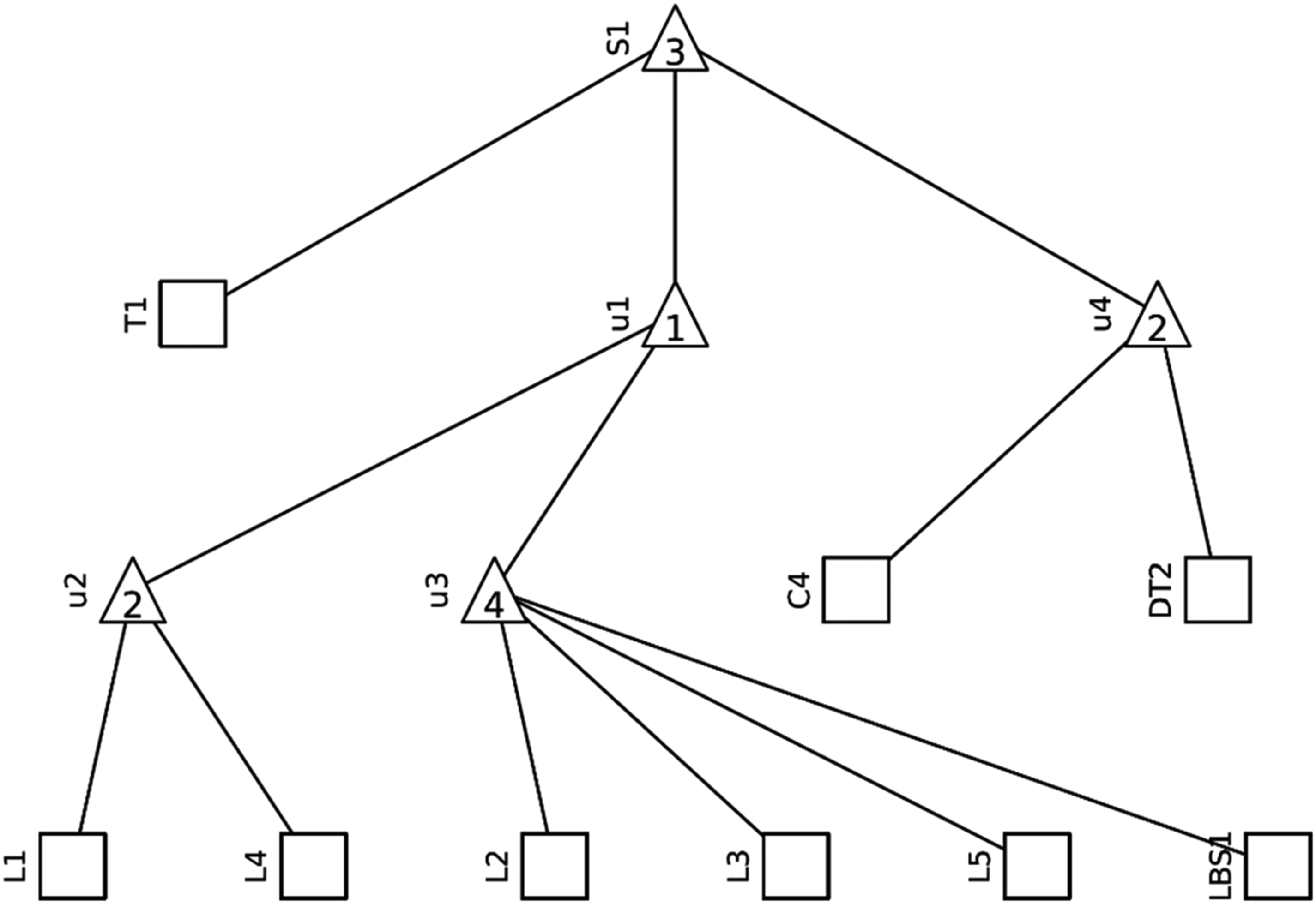
Acyclic graph of the distribution network (Vrtal et al., 2023a).

Figure 2.

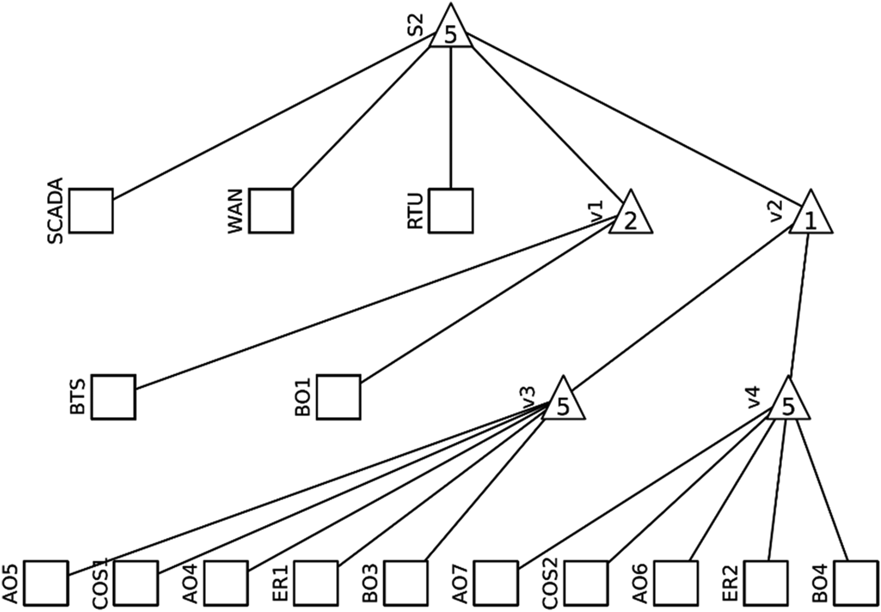
Acyclic graph of the communication grid (Vrtal et al., 2023a).

Figure 3.

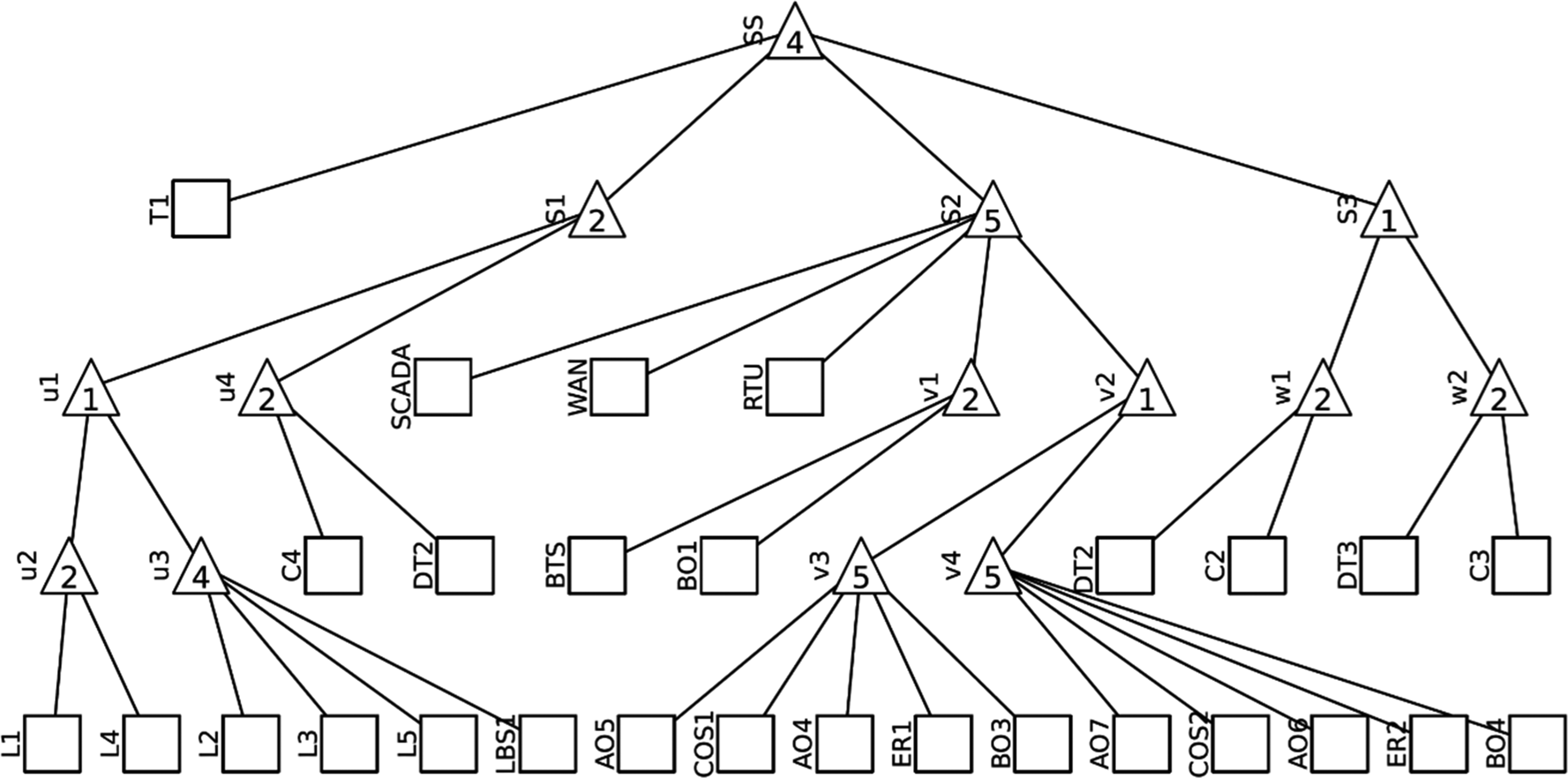
Acyclic graph of the interconnected grid (Vrtal et al., 2023a).

Each of these network elements is described by two values. The first is MTBF, which describes the expected lifetime of an element, that is, the average duration it functions before requiring repair or replacement. The second is MTTR, which specifies the average time needed to repair or replace an element. These values, determined in Vrtal et al. (2023b), are listed in Table 1.

Table 1.

Characteristic values of the grids’ components.

Component	MTBF (h)	MTTR (h)
Transformer T1 (110/22 kV)	26,310.709	4.403
Transformer DT2 (22/0.4 kV)	43,800.361	0.361
Transformer DT3 (22/0.4 kV)	43,800.361	0.361
Load break switch LBS1 (22 kV)	224,621.087	5.702
Overhead line L1 (22 kV)	398,193.235	11.417
Overhead line L2 (22 kV)	398,193.235	11.417
Overhead line L3 (22 kV)	398,193.235	11.417
Overhead line L4 (22 kV)	398,193.235	11.417
Overhead line L5 (22 kV)	398,193.235	11.417
Underground cable C2 (0.4 kV)	46,190.263	85.000
Underground cable C3 (0.4 kV)	46,190.263	85.000
Underground cable C4 (0.4 kV)	46,190.263	85.000
Edge router ER1	16,246.780	0.780
Edge router ER2	16,246.780	0.780
Core optical switch COS1	5,000,014.000	14.000
Core optical switch COS2	5,000,014.000	14.000
Aerial optic fibre AO4	175,000.000	6.000
Aerial optic fibre AO5	175,000.000	6.000
Aerial optic fibre AO6	175,000.000	6.000
Aerial optic fibre AO7	175,000.000	6.000
Buried optic fibre BO1	2,630,000.000	12.000
Buried optic fibre BO3	2,630,000.000	12.000
Buried optic fibre BO4	2,630,000.000	12.000
Remote terminal unit (RTU)	100,048.000	48.000
SCADA operation and data centre	175,200.000	184.600
Base transmitting station (BTS)	100,000.000	4.000
Wide area network (WAN)	100,000.000	4.000

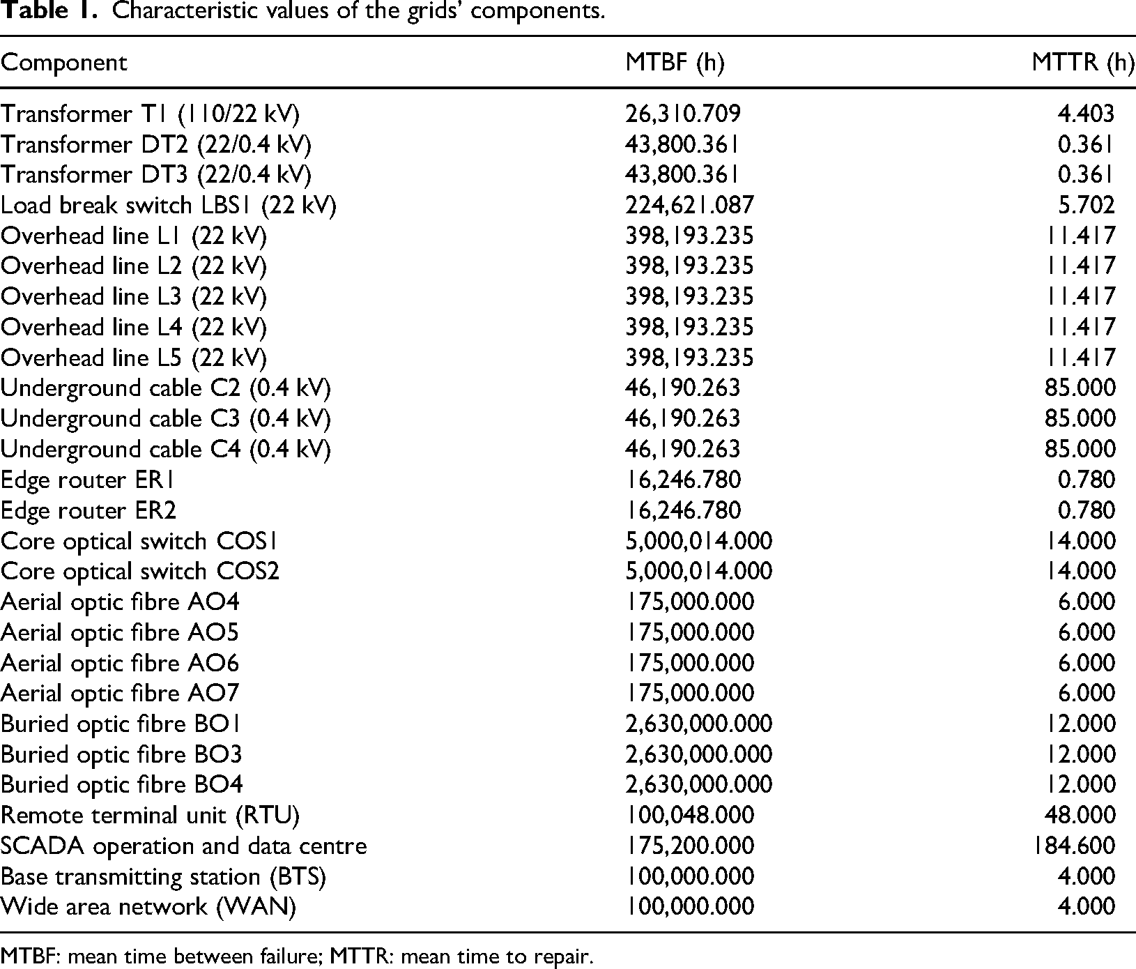
MTBF: mean time between failure; MTTR: mean time to repair.

Furthermore, it is necessary to consider the ageing of the entire system. For this purpose, the Weibull distribution is used in the modelling. The density function of the Weibull distribution is given in equation (1):

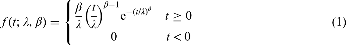
f (t; λ, β) = {\begin{matrix} \frac{β}{λ} {(\frac{t}{λ})}^{β - 1} e^{- {(t / λ)}^{β}} & t \geq 0 \\ 0 & t < 0 \end{matrix}

(1)

The shape parameter β controls how the occurrence of errors will behave. If β = 1, errors have a constant incidence. In the case of β = 2, the errors have a linear increase in occurrence, which is commonly associated with the ageing of the system. For the calculation of our systems, we consider β = 2, as we acknowledge the influence of ageing, since the times for MTBF are quite long. The scaling parameter λ determines the lifetime of a given component. The link between the parameter λ and the MTBF value is given in equation (2), where Γ(x) is the gamma function.

MTBF = λ \cdot Γ (1 + \frac{1}{β})

(2)

Literature overview

Already available methods for addressing the reliability of these systems were developed:

Ruijters and Stoelinga (2015) perform a thorough examination of the fault tree analysis and review more than 150 papers to provide a comprehensive overview of fault trees, and they further extend the knowledge by including variations such as dynamic and repairable fault trees.

Nagaraju et al. (2017) focus on cybersecurity, start with the fault trees, further expand them with event tree and attack tree, and add another method in the form of Petri nets and Markov modelling.

Another very thorough examination of various reliability, availability, maintainability, and security papers focused on the critical infrastructure is presented by Pirbhulal et al. (2021), where 1513 records published between 2011 and 2020 are identified with applications in energetics, networking, or industry. They are focusing on various questions, such as whether critical infrastructure is needed, how reliability, availability, maintainability, and security analysis are utilized for protection, what approaches are used for the analysis and how they are performing, what types of infrastructure are analysed, and what are the advantages and disadvantages of reviewed studies.

Aslansefat et al. (2020) provide a brief description of the dynamic fault tree (DFT) methodology and review many prominent DFT analysis techniques such as Markov chains, Petri Nets, and Bayesian networks.

Lazarova-Molnar et al. (2017) provide a holistic overview and identify challenges of reliability modelling in cyber-physical systems (CPSs). They present the specificities of reliability and fault modelling for all three paradigms that comprise CPS: hardware, software, and humans, and discuss the challenges related to their combination for providing a holistic approach to CPS reliability modelling.

Learning repairable multi-state fault trees from time series data of faults is introduced by Niloofar and Lazarova-Molnar (2023). The methodology can analyse reliability and maintainability distributions other than exponential. The methodology can be used for estimating the system’s future reliability and the fault tree structure.

Baklouti et al. (2020) focus on generating DFTs for systems with redundancies, which are widely used in safety-critical systems to enhance reliability. They propose a redundancy profile and generate DFTs from system models automatically.

As part of this work, a comparison of available studies addressing similar issues was conducted, as presented in Table 2.

Table 2.

Comparison of existing studies and articles.

Paper/work	Application area	Open source	HPC	Interconnected model	Availability estimation
Ruijters and Stoelinga (2015)	General fault tree analysis	Partially	No	No	Yes
Nagaraju et al. (2017)	Cyber risk management	Partially	No	Partially	Partially
Pirbhulal et al. (2021)	Critical infrastructure protection	Partially	No	Yes	Yes
Garg and Ram (2020)	Reliability management and engineering	No	No	No	Yes
Lazarova-Molnar et al. (2017)	Cyber-physical systems reliability	No	No	Yes	Yes
Niloofar and Lazarova-Molnar (2023)	Data-driven repairable fault trees	Partially	No	No	Yes
Baklouti et al. (2020)	Dynamic fault tree generation	No	No	No	No
Baklouti et al. (2017)	free and open source fault tree analysis tools survey	Yes	No	No	Partially
Morozov et al. (2019)	Stochastic model-based reliability & resilience analysis	Yes	No	No	Partially
Hensel et al. (2022)	Probabilistic model checker storm	Yes	No	No	Partially
R Core Team (2021)	Statistical computing environment	Yes	Partially	No	No
Silkworth (2023)	Fault trees for risk and reliability analysis	Yes	No	No	Yes
Niloofar et al. (2022c)	Fault tree analysis based on proxel simulation	Yes	No	No	Yes
Niloofar et al. (2022a)	ftaproxim - R package for proxel-based simulation of fault trees	Yes	No	Partially	Yes
Niloofar et al. (2022b)	Proxel-based simulation of fault trees in R	Yes	No	No	Yes
Vrtal et al. (2023b)	Critical parameters & interdependencies in smart grids	No	No	Yes	No
Vrtal et al. (2023a)	Time-dependent unavailability exploration	No	No	Yes	Yes
This study	Interconnected power & communication networks	Yes	Yes	Yes	Yes

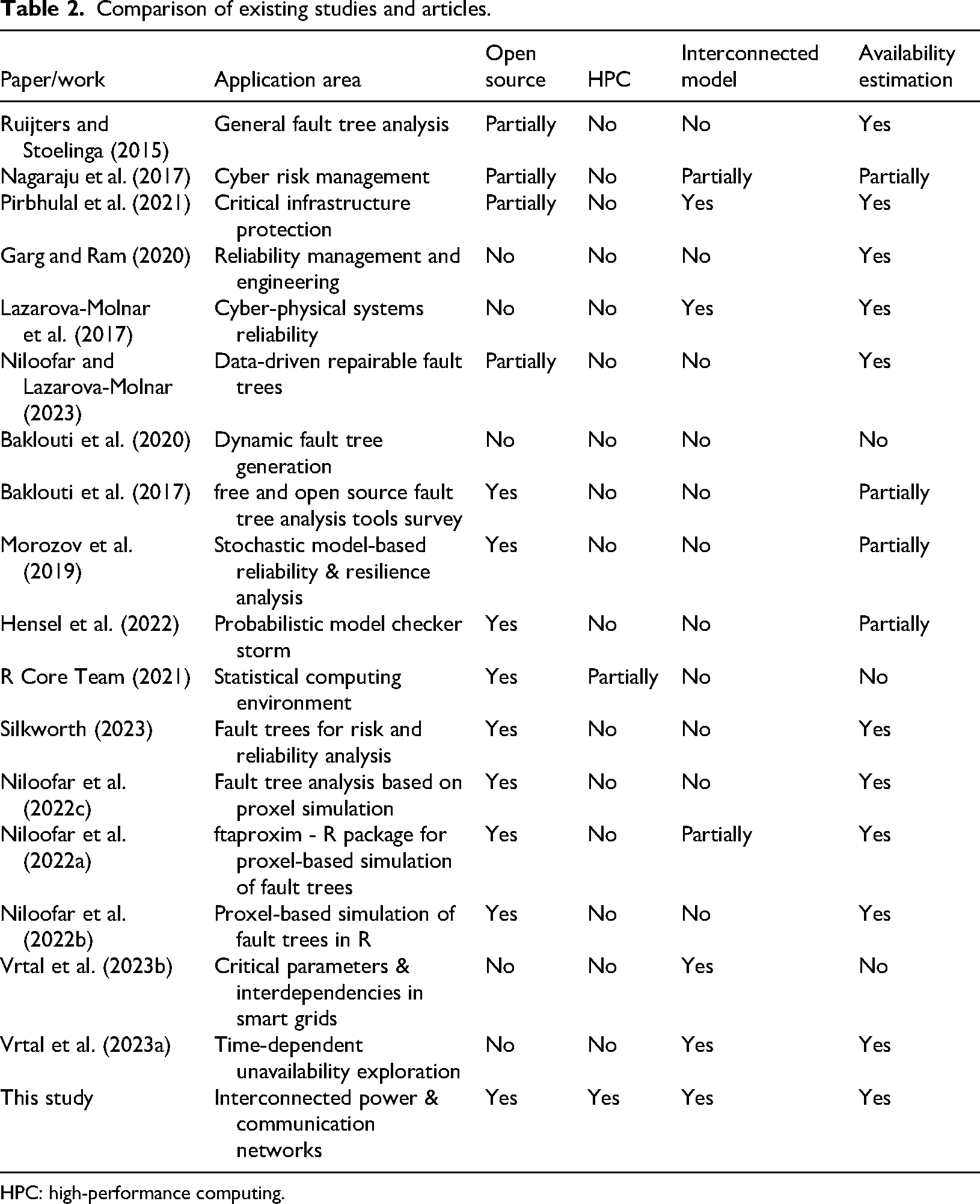
HPC: high-performance computing.

The comparative analysis presented in Table 2 highlights the key differences between the current work and a range of existing studies on fault tree analysis, reliability modelling, and critical infrastructure assessment. While prior works cover various aspects such as general fault tree analysis (Ruijters and Stoelinga, 2015), cyber risk management (Nagaraju et al., 2017), or resilience in CPSs (Lazarova-Molnar et al., 2017), they tend to focus either on theoretical foundations, isolated systems, or offer only partial consideration of open-source tools. Several references, including Baklouti et al. (2017), Silkworth (2023) and Niloofar et al. (2022c), introduce or review open-source R packages such as FaultTree or ftaproxim, yet they do not evaluate their performance in complex interconnected environments or under HPC conditions.

In contrast, the novel method presented here fills a significant gap by systematically evaluating the time-dependent unavailability of large-scale interconnected power and communication networks using open-source R packages. It stands out by conducting the analysis on a supercomputer, thereby assessing both computational scalability and accuracy.

Furthermore, it offers a direct comparison with commercial software and provides a detailed analysis of key tool parameters.

Novel method

To the best knowledge of the authors of this study, no prior work delivers this level of integration combining open-source availability, HPC scalability, interconnected infrastructure modelling, and unavailability estimation within a unified, reproducible framework. This represents a novel and valuable contribution to the field.

As mentioned in the introduction, two packages capable of computing the (un)availability in the language R (R Core Team 2021) were chosen for this study. The first package, FaultTree (Silkworth 2023), works with the tree structure and uses the gate-to-gate approach to obtain the results (Doelp et al., 1984). The individual elements are characterized by the MTBF and MTTR. The relations between the elements are realized with the AND and OR gates. The reliability of individual nodes is computed in a subsequent calculation. The output is presented in an understandable tree structure, as was entered on the input. The software is limited to the computation of asymptotic unavailability. While knowing the theoretical unavailability can provide useful insight into the expected behaviour of the system, our use case required more detailed knowledge of the unavailability throughout the operation time. Still, this package is suitable for solving simpler problems, and, therefore, it is good to familiarize oneself with the output format and presentation of results. It can also serve as confirmation of the results. Most importantly, it allows us to work on the tree structure, such as visualization, that can be used to double-check the correct definition of the problem. It can also compute the minimal cut sets, a useful feature used by the following package.

The other package, ftaproxim (Niloofar et al., 2022c), calculates and plots instantaneous unavailabilities of basic events along with the top event (TE) of fault trees. All methods, based on the proxel-based simulation, are derived from Niloofar et al. (2022c). This type of simulation was introduced by Horton (2002) as a state-space-based analysis method for Stochastic Petri Nets, which are analysed using DTMCs as underlying models. It computes the probabilities of all potential state changes in a deterministic way, similar to Markov chains, but is not restricted to exponential distributions. Supplementary variables are used to store the age information of enabled state transitions. The probability of state changes is computed using the instantaneous hazard rate functions of the associated distributions. The age information is stored together with the discrete state and the probability, forming a probability element (proxel). A proxel is defined as a tuple $(s, a, p)$ , where s represents the discrete state, a stands for the age of the proxel, and p denotes the probability of being in state s of age a at time t. The proxel-based simulation method deterministically generates and tracks all possible developments of system behaviour over discrete time steps. Rare events and all reachable system states are guaranteed to be considered. For this purpose, the transitions are governed by the hazard rate h(t). The hazard rate is defined as $h (t) = f (t) / [1 - F (t)]$ , where f(t) is the probability density function (pdf) and F(t) is the cumulative distribution function. The probability of transitioning from state s to a new state s′ at time $t + Δ t$ is given equation (3):

p_{t + Δ t} (s^{'}, 0) = p_{t} (s, a) \cdot h (a) \cdot Δ t

(3)

where h(a) represents the instantaneous hazard rate at age a and

Δ t

is the time step, and their product is the approximate probability of a transition occurring in the interval

Δ t

. The probability of remaining in the current state s and ageing by

Δ t

is represented in equation (4):

p_{t + Δ t} (s, a + Δ t) = p_{t} (s, a) \cdot (1 - h (a) \cdot Δ t)

(4)

Since these equations use the general form of the hazard function, the proxel-based simulation can accommodate arbitrary probability distributions, making the method highly flexible in the types of values it can process. Each basic element is characterized by two probability distributions, one for MTBF and one for MTTR. In this case, the MTBF follows the Weibull distribution, $MTBF \sim Weibull (λ, β)$ , and the MTTR follows the uniform distribution, $MTTR \sim Uniform (a, b)$ . Since the algorithm requires the values of the parameters, $λ$ and $β$ in case of MTBF, and a and b in case of MTTR, these values need to be computed beforehand. For the MTBF, the value of scale parameter $λ$ can be obtained from equation (5), where MTBF is the known parameter representing the component, $β$ is the chosen shape parameter and $Γ (x)$ is the gamma function

λ = \frac{MTBF}{Γ (1 + (1 / β))}

(5)

Similarly, the limits of the uniform distribution, a and b, must be calculated from the value of MTTR, defined for the uniform distribution as given in equation (6):

MTTR = \frac{a + b}{2}

(6)

Assuming that the start of the uniform distribution is fixed; $a = 0$ , then the value $b = 2 \cdot MTTR$ . The structure of the model is not entered as the whole tree, but is represented with the minimal cut sets. These are the smallest sets of given elements that will cause the system to malfunction. Given the low complexity of the presented networks, it was easy to find a minimal cut set of the model manually, but in the case of more complex networks, it will be necessary to find an algorithmic solution, which will leverage the min-cut approach. Fortunately, the previous FaultTree package is capable of computing the minimal cut sets. Furthermore, other methodology is discussed by Tang and Dugan (2004). Two parameters directly influencing the accuracy and the speed of the computation can be modified. The tolerance value serves as the cut-off value, where proxels with probabilities smaller than the given tolerance level are ignored. Lowering the value of tolerance will therefore lead to more precise computation, while demanding more computational power. The time step parameter determines the step of the algorithm, where the probabilities are computed. Increasing the time step leads to a lower number of computations and thus speeds up the process. The algorithm also requires the mission time, the length of how long the system will be monitored.

Evaluation of unavailability modelling

Results and observations

The computations in this study were performed using R programming language version 4.1.1 on a Dell G3 3500 laptop with an Intel(R) Core™ i7-10750H CPU @ 2.60 GHz, 2.59 GHz, 16 GB RAM, running Windows 10 Home. The FaultTree package was version 1.0.1, and the ftaproxim package was version 0.0.1.

This section presents the unavailability results obtained using ftaproxim for selected combinations of input parameters. For simplicity, it focuses on configurations with time steps of 1 h and 10 h, and tolerance values of 10⁻⁵ and 10⁻⁶. The following section expands the analysis through a grid search over a broader range of input combinations.

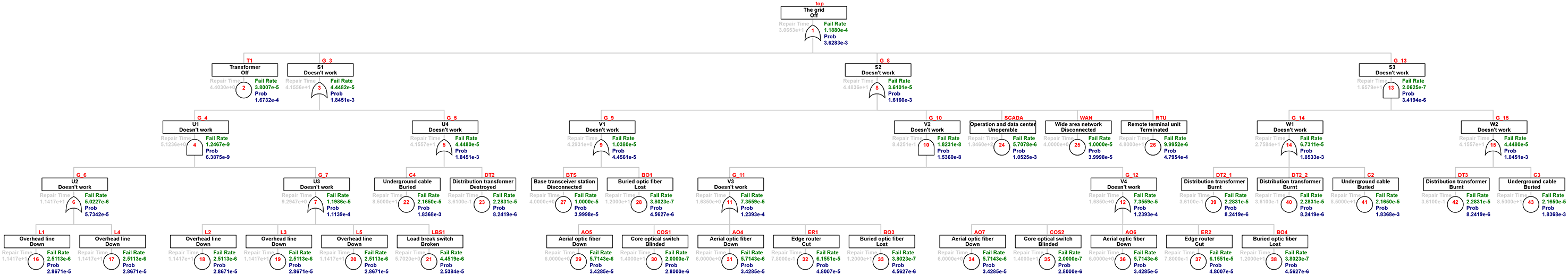
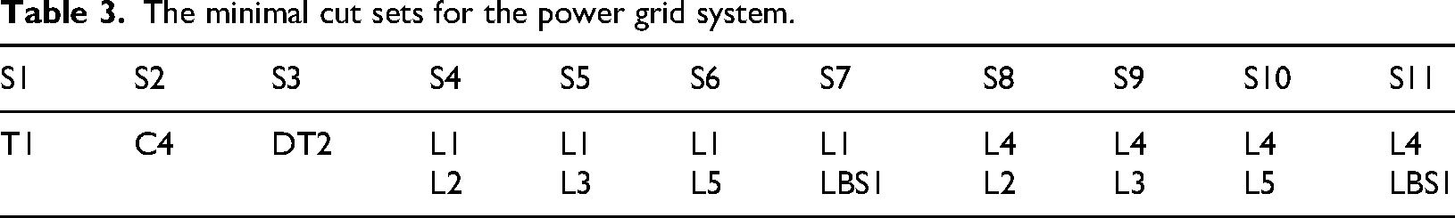
As mentioned, the FaultTree package lacks the results relevant for our case study, but the output can still be useful for the reader; therefore, they are presented here for illustration. The speed of calculation is almost instantaneous, so all three systems were solved with this package. Moreover, this package was used to compute the minimal cut set of the system. For illustration, the minimal cut set of the distribution network is shown in Table 3. Figure 4 shows the results of the unavailability estimation for the distribution network. For the specified elements, their table values are given in Table 1. Unknown nodes have the repair time, fail rate (reversed MTBF value), and Prob (probability of unavailability of the given element given the probability of failure and time until repair) calculated. The software output is comprehensible, and in addition to the overall probability of system failure, it also displays partial node failures. The results of unavailability calculations are shown in Figure 5 for the communication grid and Figure 6 for the interconnected grid, respectively.

Figure 4.

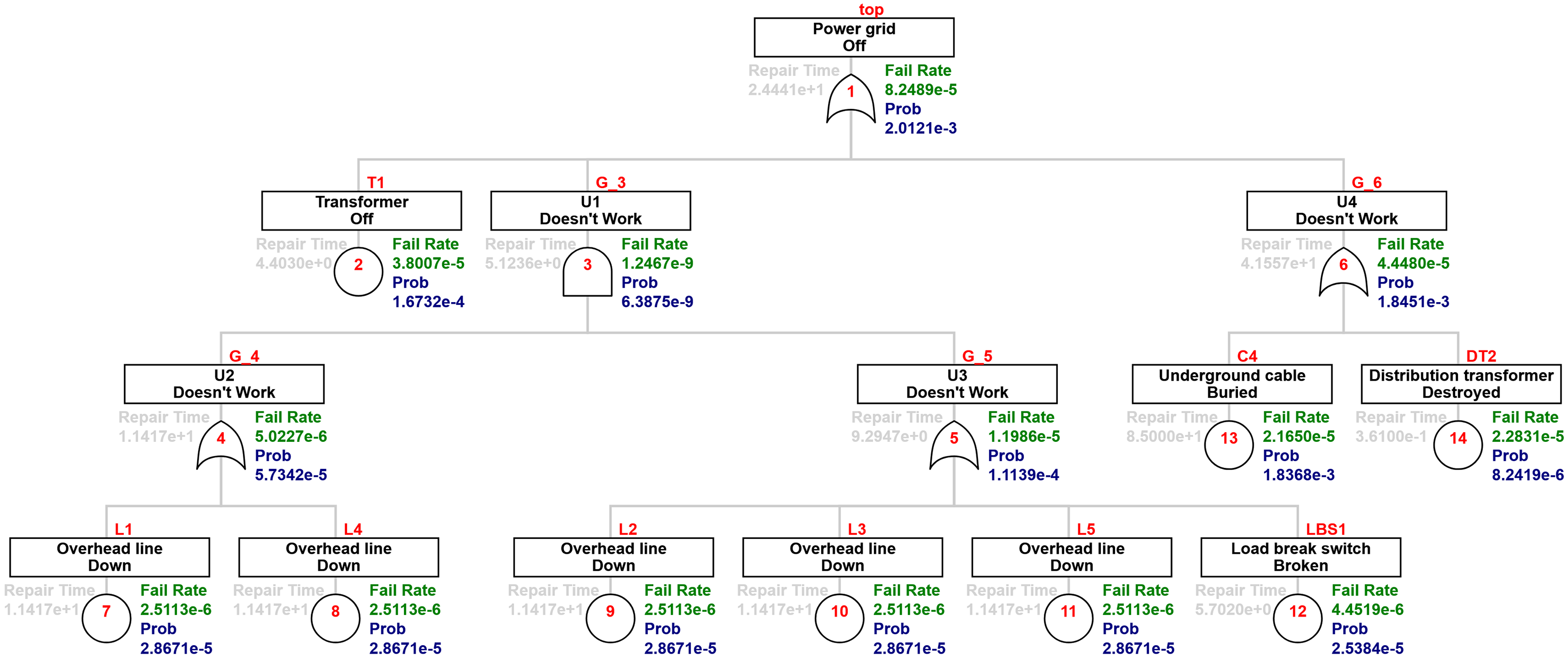
Results of the FaultTree package for the distribution network.

Figure 5.

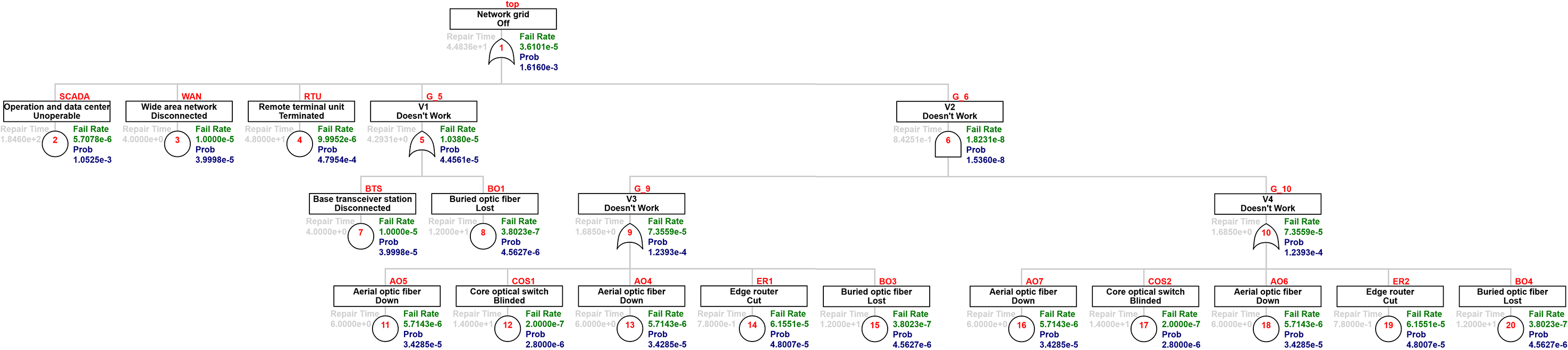
Results of the FaultTree package for the communication grid.

Figure 6.

Results of the FaultTree package for the interconnected grid.

Table 3.

The minimal cut sets for the power grid system.

S1	S2	S3	S4	S5	S6	S7	S8	S9	S10	S11
T1	C4	DT2	L1	L1	L1	L1	L4	L4	L4	L4
			L2	L3	L5	LBS1	L2	L3	L5	LBS1

For example, the results of Figure 4 show that the TE ‘Power grid off’ has a failure rate of 8.2489 × 10⁻⁵ (see the green text on the top of Figure 4), whereas the probability of this TE is 2.0121 × 10⁻³ (see the dark blue text on the top of Figure 4).

The results of the ftaproxim package were compared with the results computed beforehand in the commercial software Matlab. This result is shown in Figure 7. On the x-axis is the mission time in hours. The y-axis shows the unavailability of the system for a given time. There are two additional information added, the values for unavailability in 10,000 h and in 40,000 h. Both these values and the general shape of the unavailability in Figure 7 serve as the foundation to which we later compare our results obtained in ftaproxim package.

Figure 7.

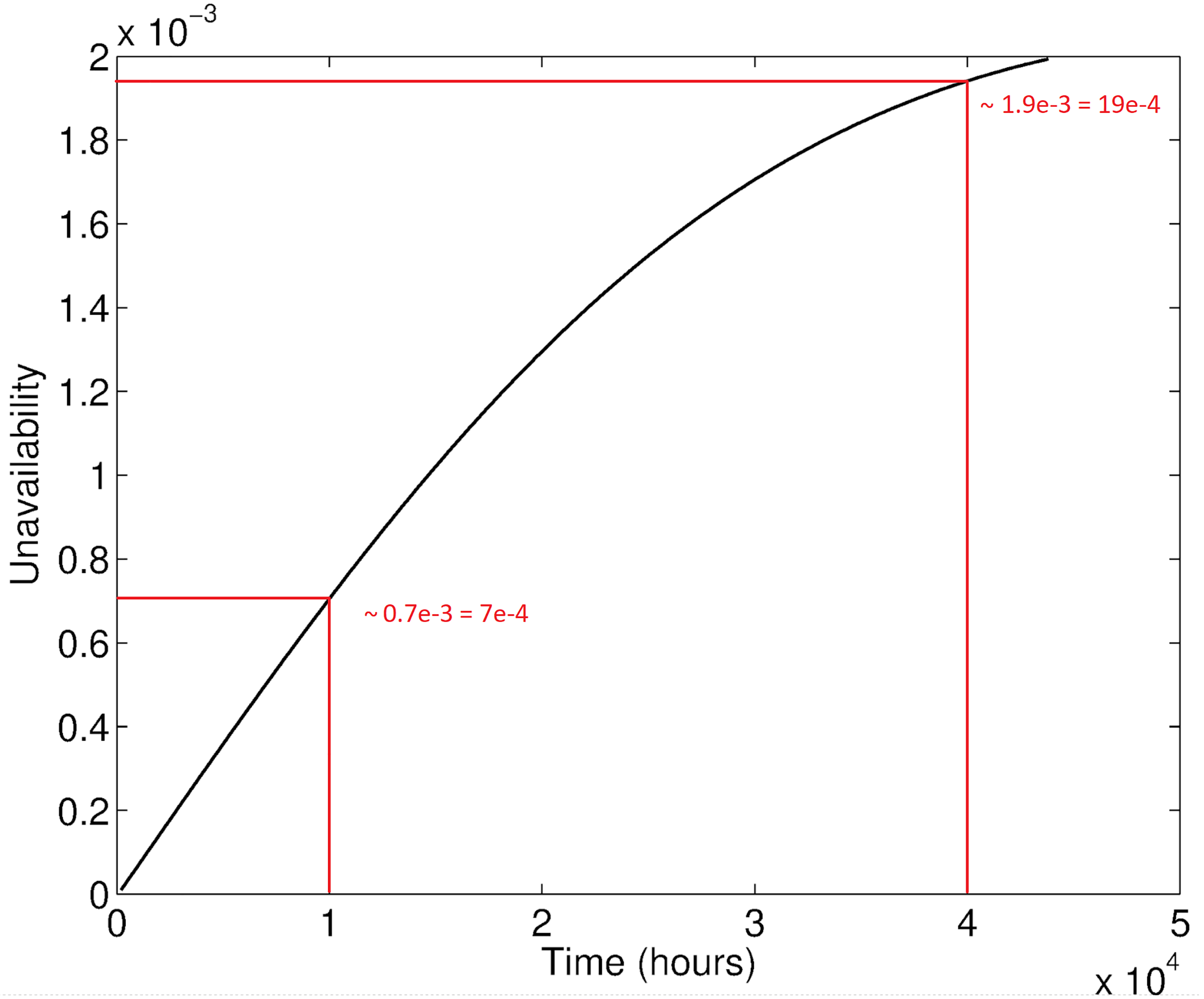
Referential result with indicated unavailability values for 10,000 and 40,000 h.

Unavailability results for a 1 h step with tolerance 10⁻⁶ for a 10,000 h mission time

In the initial phase of the ftaproxim package testing, an operating time of 10,000 h with a step of 1 h and a tolerance of 10⁻⁶ was tested. Already at this stage, it was found that the calculation takes a significantly long time (approximately 26 h). Therefore, in the second step, we looked at alternatives that could speed up the calculation time, namely increasing the step or decreasing the tolerance. Expectedly, the price for speeding up the algorithm is a reduction in the accuracy of the result. Due to the long calculation times, we present the results only for the distribution network.

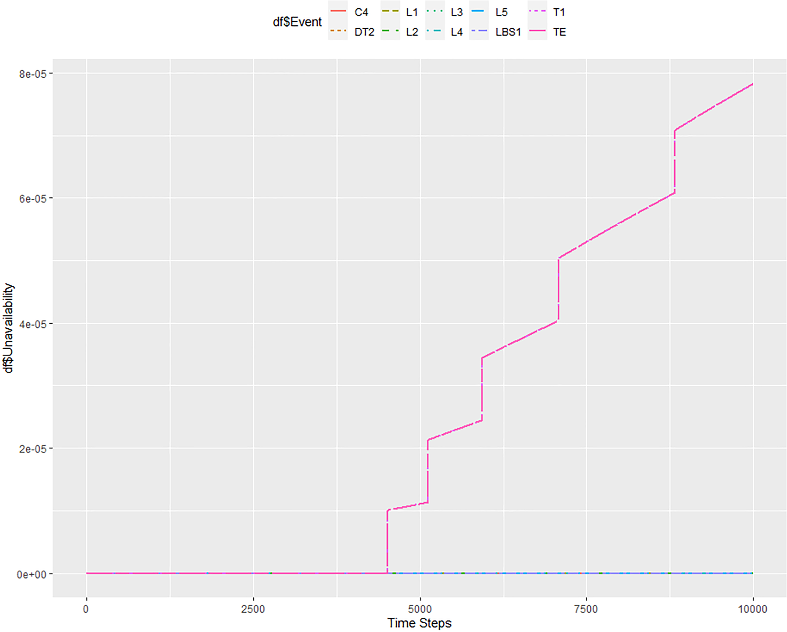
The first calculation by the ftaproxim package was for a length of 10,000 h with a step of 1 h and a tolerance of 10⁻⁶. The duration of the calculation was approximately 26 h. Figure 8 shows the system unavailability values for this period. The TE, representing the unavailability of the entire system, is denoted in magenta. It can be seen from the graph that the unavailability of the entire system is roughly 7 × 10⁻⁴ in 10,000 h. Comparing Figures 7 and 8 side by side, it can be concluded that the obtained values for the 10,000 h match. Additionally, the almost linear characteristic of unavailability is preserved as well. Ftaproxim package displays another useful information about the unavailability of all the components that are present in the system. Based on the Matlab computation, it is known that the components C4 and T1 have the largest share of system unreliability. Figure 8 shows that this also corresponds to the results obtained using the ftaproxim package.

Figure 8.

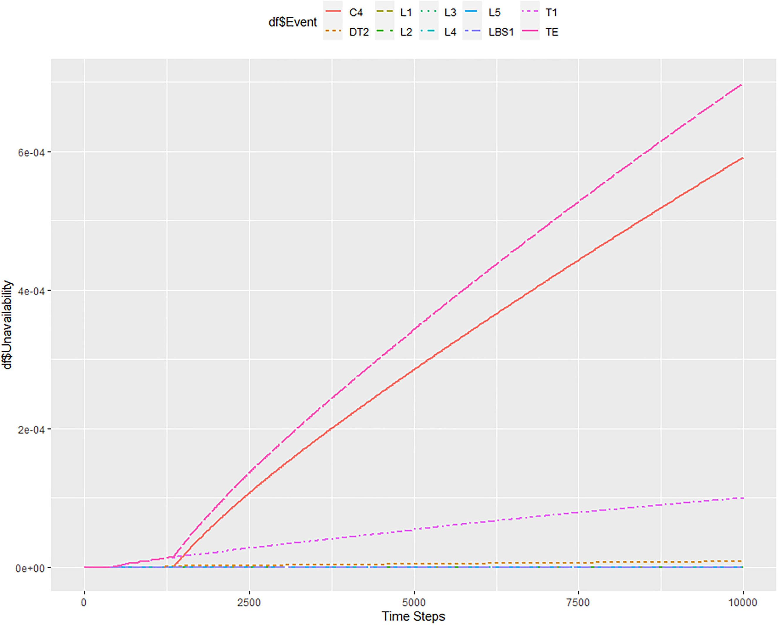
Results of unavailability modelling for 10,000 h with a step = 1 h and tolerance = 10⁻⁶.

Unavailability results for a 1 h step with tolerance 10⁻⁵ for a 10,000 h mission time

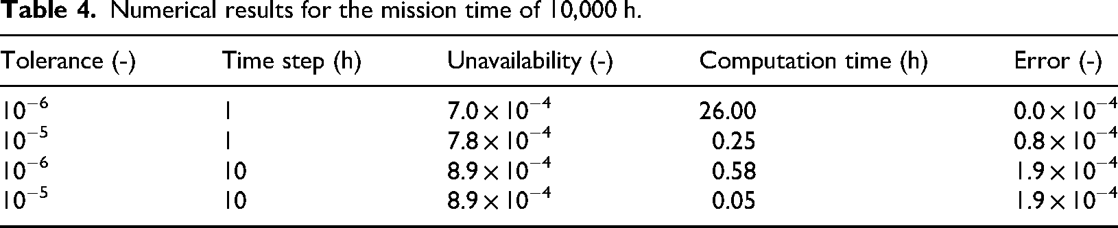
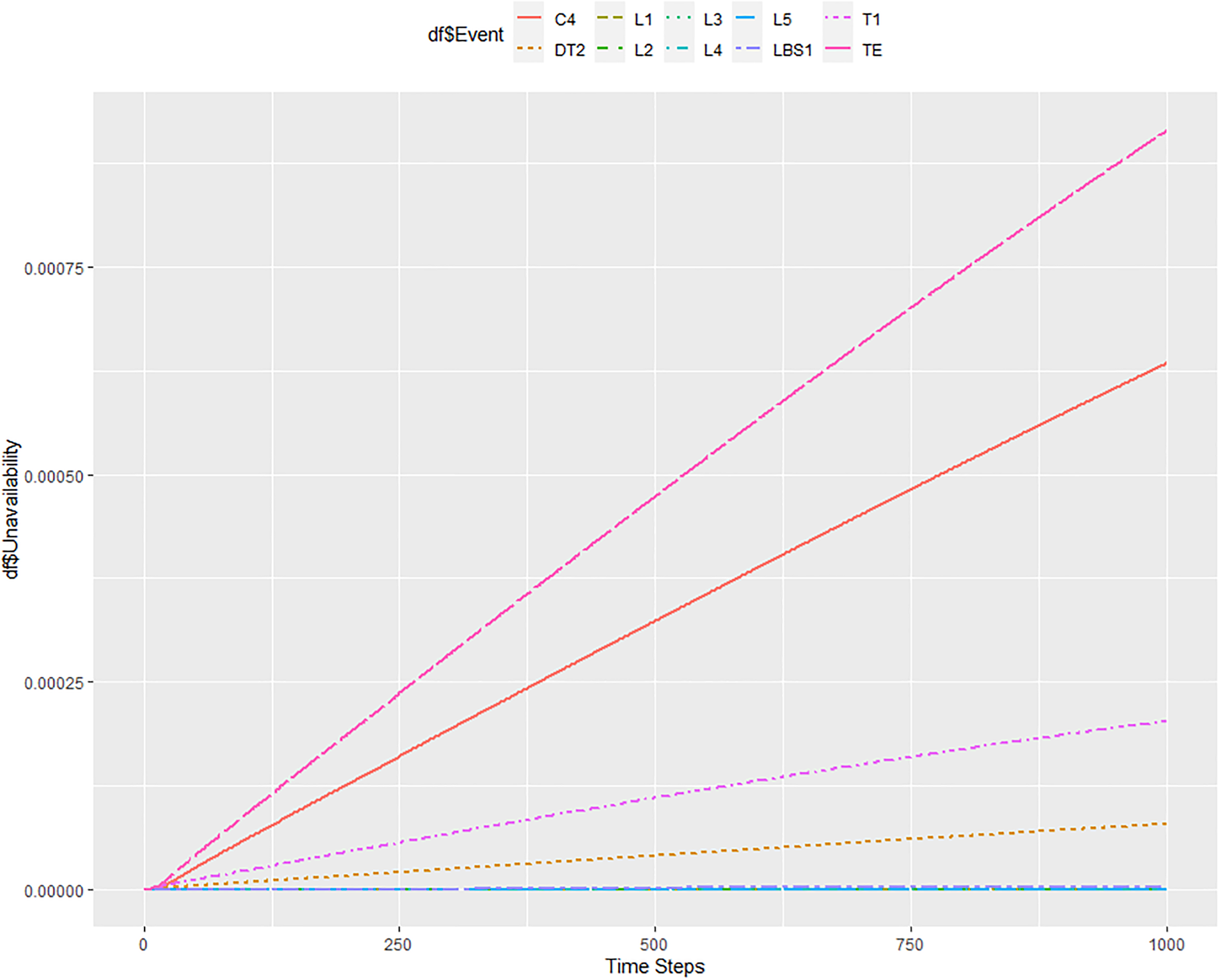
To speed up the calculations of the ftaproxim package, we first tried to reduce the tolerance to 10⁻⁵. This significantly accelerated the calculation to about 15 min. Figure 9 shows the result of this calculation. It can be seen that lowering the tolerance leads to a less smooth unavailability curve. System unavailability in 10,000 h is 7.8 × 10⁻⁴, that is, relatively close to the target value, which is 7 × 10⁻⁴, as can be seen in Figure 7 and Table 4 for comparison. In this setting, the ftaproxim package loses information about the increased unavailability of elements C4 and T1, as given in Figure 9, which is a very important information loss.

Figure 9.

Results of unavailability modelling for 10,000 h with a step = 1 h and tolerance = 10⁻⁵.

Table 4.

Numerical results for the mission time of 10,000 h.

Tolerance (-)	Time step (h)	Unavailability (-)	Computation time (h)	Error (-)
10⁻⁶	1	7.0 × 10⁻⁴	26.00	0.0 × 10⁻⁴
10⁻⁵	1	7.8 × 10⁻⁴	0.25	0.8 × 10⁻⁴
10⁻⁶	10	8.9 × 10⁻⁴	0.58	1.9 × 10⁻⁴
10⁻⁵	10	8.9 × 10⁻⁴	0.05	1.9 × 10⁻⁴

Unavailability results for a 10 h step with tolerance 10⁻⁶ for 10,000 h mission time

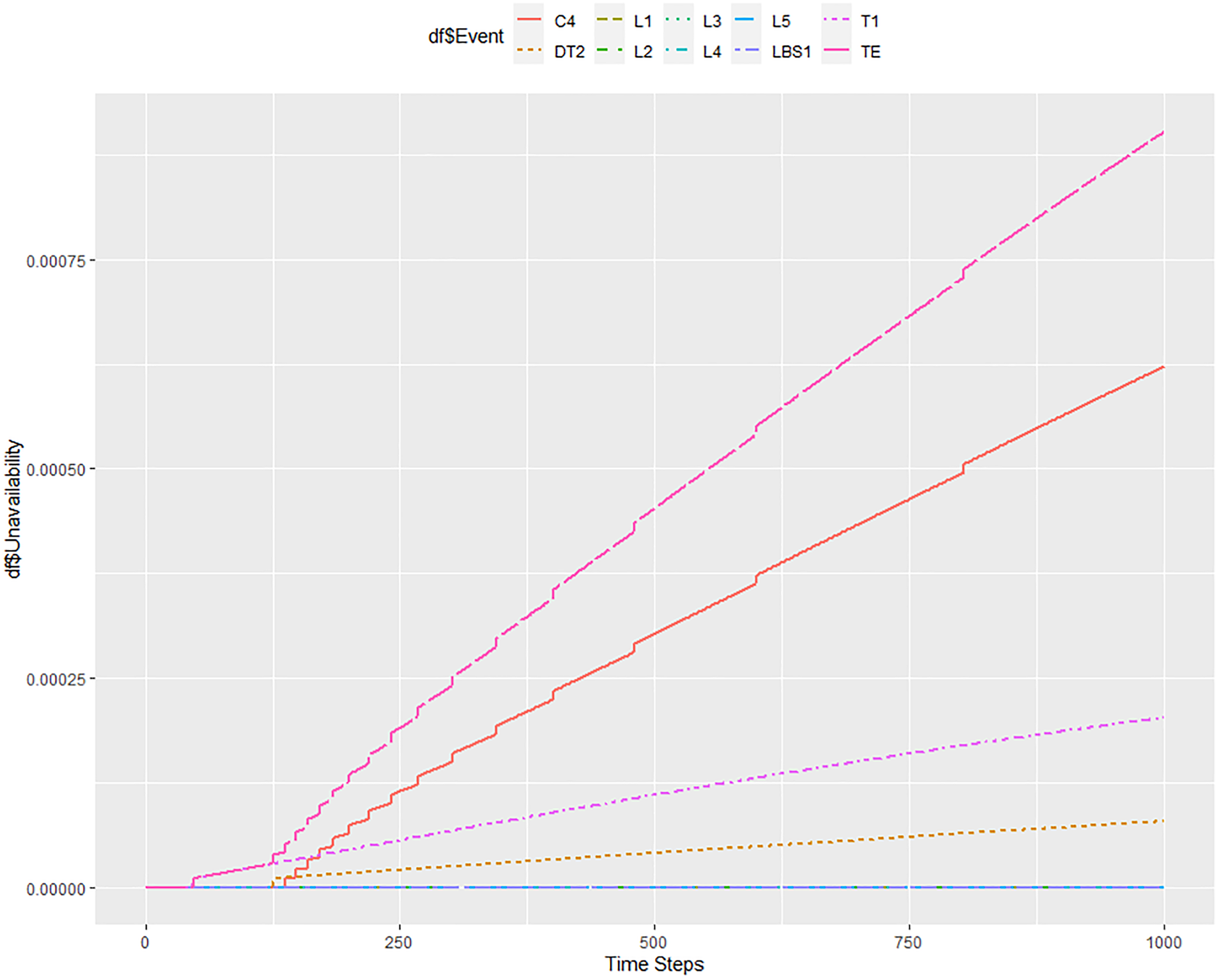
The subsequent Figure 10 shows the result for the situation where we increase the step to 10 h while keeping the 10⁻⁶ tolerance. The result of system unavailability in 10,000 h is roughly 8.9 × 10⁻⁴. The information about the increased unavailability of C4 and T1 elements remained here, and the unavailability of the DT2 element was significantly increased. The total calculation time was about 35 min.

Figure 10.

Results of unavailability modelling for 10,000 h with a step = 10 h and tolerance = 10⁻⁶.

Unavailability results for a 10 h step with tolerance 10⁻⁵ for 10,000 h mission time

Figure 11 shows a situation where the tolerance has been reduced to 10⁻⁵ and the step has been increased to 10 h. The result of system unavailability at 10,000 h is roughly 8.9 × 10⁻⁴, the same as in the previous case. Here, the information about the increased unavailability of elements C4 and T1 was preserved. The total calculation time took a few minutes.

Figure 11.

Results of unavailability modelling for 10,000 h with a step = 10 h and tolerance = 10⁻⁵.

From these experiments, it is evident that the greatest effect on the reduction of computing time is the reduction of tolerance, as we will also lose information about the unavailability of other elements. Increasing the time step preserves the precision of unavailability calculations. The calculation time is still significantly lower compared to the original model, which took 26 h. Numerical results are for higher clarity summarized in Table 4. There is also a column error included, which is defined as the absolute distance between the ftaproxim result and the Matlab result.

Note that in the case of step = 10 h, the values on the x-axis need to be multiplied by 10; that is, if the value on the x-axis is 100, it corresponds to a time of 1000 h.

Unavailability results for a 1 h step with tolerance 10⁻⁶ for 40,000 h mission time

This study proceeded with the unavailability modelling in the same fashion for the observed period of 40,000 h as well. The unavailability calculation for a time step of 1 h and a tolerance of 10⁻⁶ is unacceptably slow, as it took about 11 days and ended with an error message of insufficient memory.

Unavailability results for a 1 h step with tolerance 10⁻⁵ for 40,000 h mission time

For the above-mentioned reason, Figure 12 shows the setting of 1 h step and 10⁻⁵ tolerance. The calculation time was about 8 h. Here we already see the information about the increased unreliability of elements T1 and C4. We can notice that the increased unreliability of T1 was also present in the previous calculation; it just perfectly merged with the output of the entire system. The unreliability of the C4 element becomes apparent only after approximately 15,000 h. The probability of failure in 40,000 h is about 9.4 × 10⁻⁴, which is almost half of the result of 19 × 10⁻⁴, as can be seen in Figure 7. It is clear that this setting of the ftaproxim package did not provide sufficiently accurate results. Thus, our experiments show that the unavailability calculations cannot be precisely estimated by the open ftaproxim package in this case.

Figure 12.

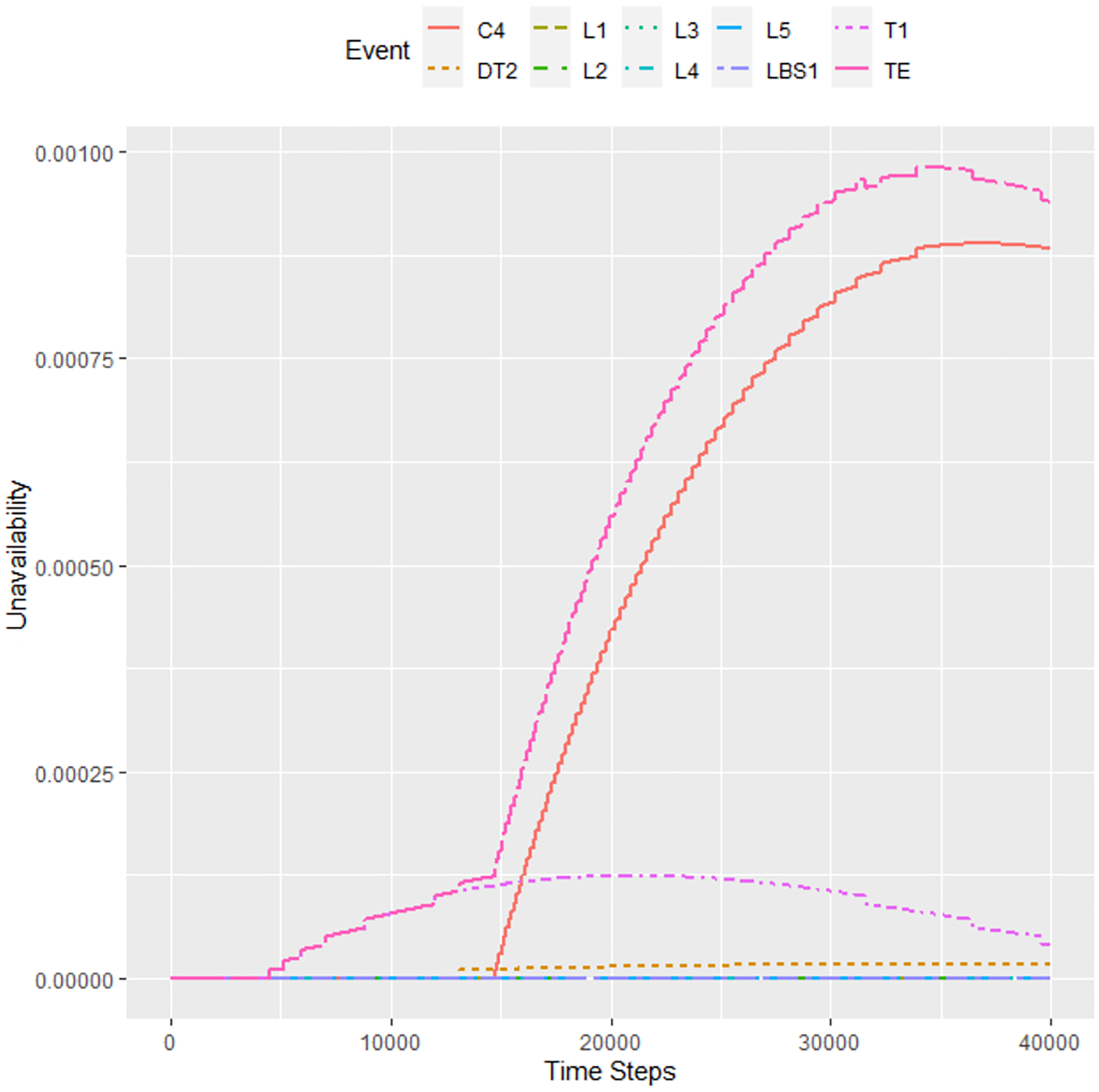
Results for 40,000 h with a step = 1 h and tolerance = 10⁻⁵.

Unavailability results for a 10 h step with tolerance 10⁻⁶ for 40,000 h mission time

Figure 13 shows a situation with a step of 10 h and a tolerance of 10⁻⁶. The calculation took almost 50 h. In 40,000 h, the probability of unavailability is about 18 × 10⁻⁴, that is, a value very close to the referenced Matlab result.

Figure 13.

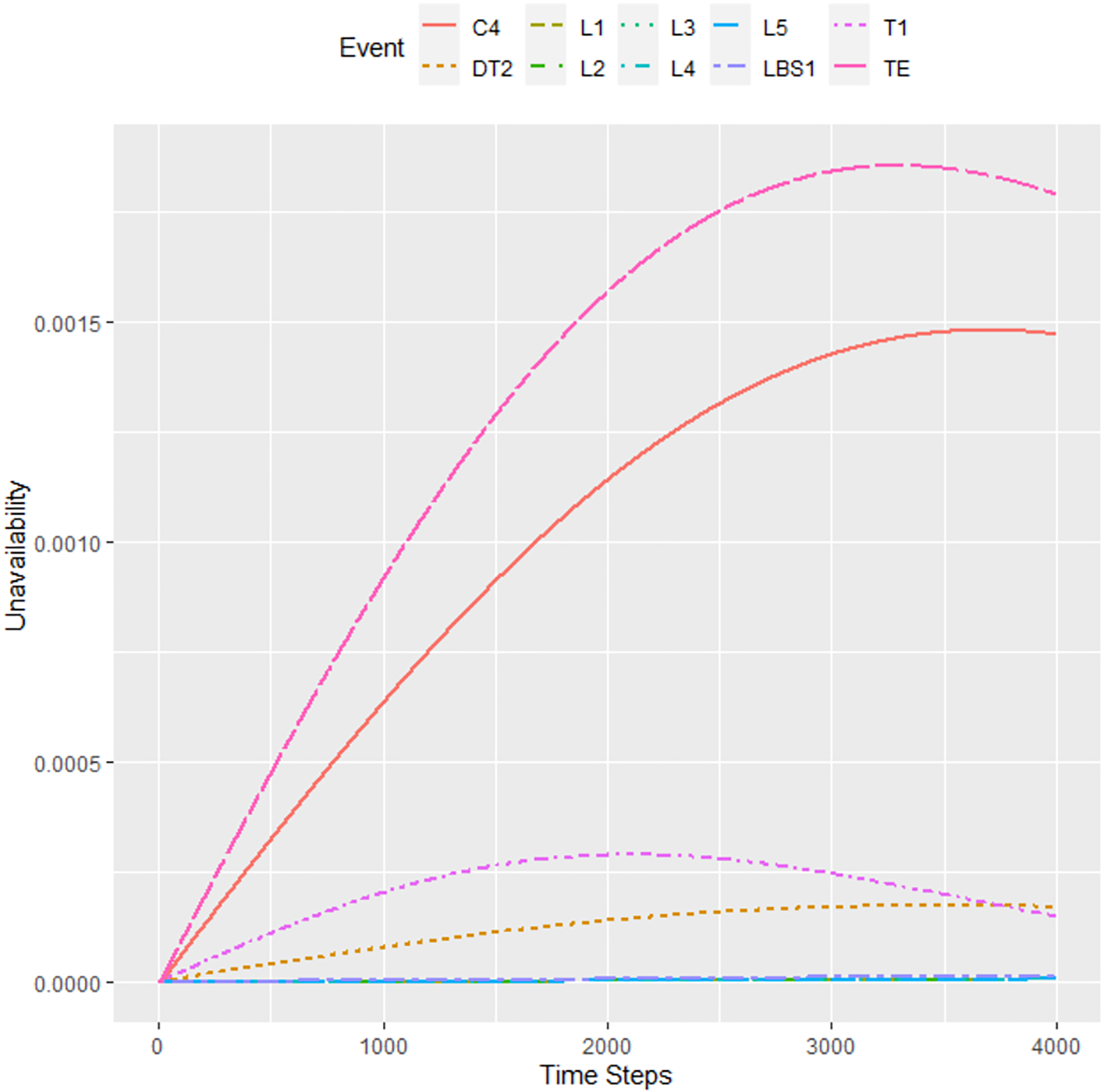
Results for 40,000 h with a step = 10 h and tolerance = 10⁻⁶.

Unavailability results for a 10 h step with tolerance 10⁻⁵ for 40,000 h mission time

Finally, Figure 14 shows the calculation result for the variant where the tolerance was reduced to 10⁻⁵ and the step was increased to 10 h. The system unavailability in 40,000 h is approximately 17.5 × 10⁻⁴. The calculation for 40,000 h also confirmed the increased unavailability of elements C4 and T1, in addition to DT2. The total calculation time was about 5 h.

Figure 14.

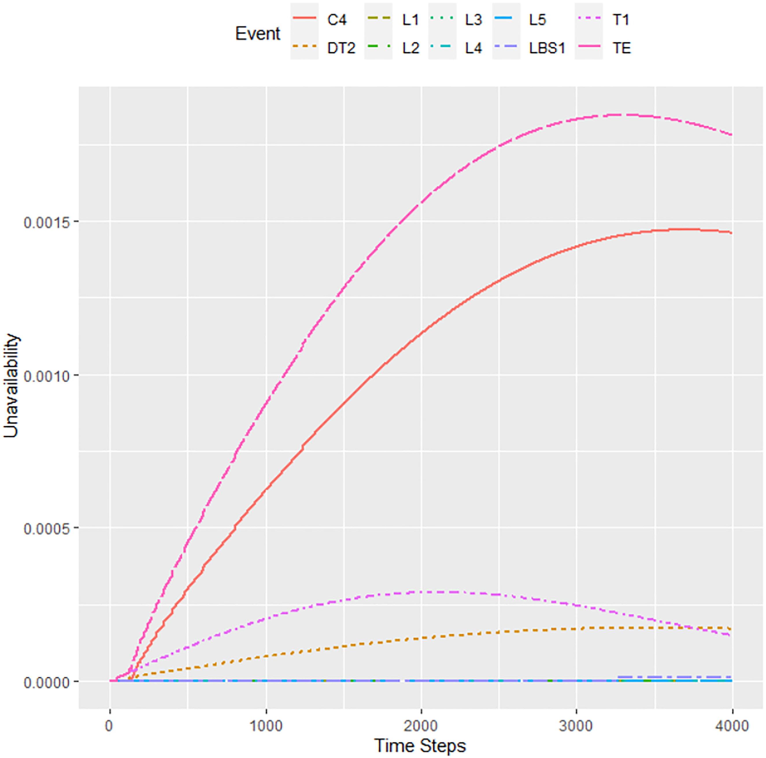
Results for 40,000 h with a step = 10 h and tolerance = 10⁻⁵.

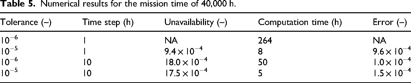
Here, we can conclude that tolerance has the highest influence on the correctness of the unavailability solution. Tolerance values of 10⁻⁵ are very far from the Matlab results. On the contrary, increasing the time step to 10 h gives a result that is very close to the expected results, and this result is still obtainable in a reasonable amount of time. Naturally, the fastest computation time is achieved when both the time step and lower the tolerance were increased. It is, however, peculiar that with this approach, a much better result is obtained than in the case where only tolerance was decreased. This is probably because of the propagation of the error. A higher value of the time step leads to fewer internal calculations and, therefore, the influence of the error is not as pronounced. Summary of the results is in Table 5.

Table 5.

Numerical results for the mission time of 40,000 h.

Tolerance (–)	Time step (h)	Unavailability (–)	Computation time (h)	Error (–)
10⁻⁶	1	NA	264	NA
10⁻⁵	1	9.4 × 10⁻⁴	8	9.6 × 10⁻⁴
10⁻⁶	10	18.0 × 10⁻⁴	50	1.0 × 10⁻⁴
10⁻⁵	10	17.5 × 10⁻⁴	5	1.5 × 10⁻⁴

Grid search of input parameters of the ftaproxim R package

Due to the high computational demands discussed earlier, the computer codes for unavailability estimations were tested on the Barbora supercomputer cluster and the petascale system Karolina hosted by IT4Innovations of VSB – Technical University of Ostrava, the Czech Republic. Karolina, with a theoretical peak performance of 15.7 petaflop/s, qualifies as a peta-scale system (Karolina infrastructure), whereas Barbora has the theoretical peak of 849 teraflop/s (Barbora infrastructure). The codes used in the numerical experiments, validated on both supercomputers, are provided in Appendices A and B and Electronic Appendices A and B.

It was noted that the unavailability estimation computation time relies on the combination of the input parameters, time step and tolerance. To get a better understanding of how the input parameters influence the computation time, the grid search was performed on the distribution network model. The sensible values were chosen for both the step and tolerance, and every combination was then computed.

The values chosen for step = {1, 2, 4, 5, 8, 10, 20, 40, 50, 80, 100} and tolerance = {1 × 10⁻³, 1 × 10⁻⁴, 1 × 10⁻⁵, 1 × 10⁻⁶, 1 × 10⁻⁷} result in a total 11 × 5 = 55 unique parameter combinations. These were executed in parallel on the supercomputer as 55 independent processes. The open-source Python code is provided in Electronic Appendix A, while the open-source R code is available in Electronic Appendix B.

All combinations were computed simultaneously on the Barbora supercomputer cluster. The maximum computation time was limited to 48 h. The results are shown in the heat map presented in Figure 15. White parts show a combination that was not computed in the given time limit (48 h).

Figure 15.

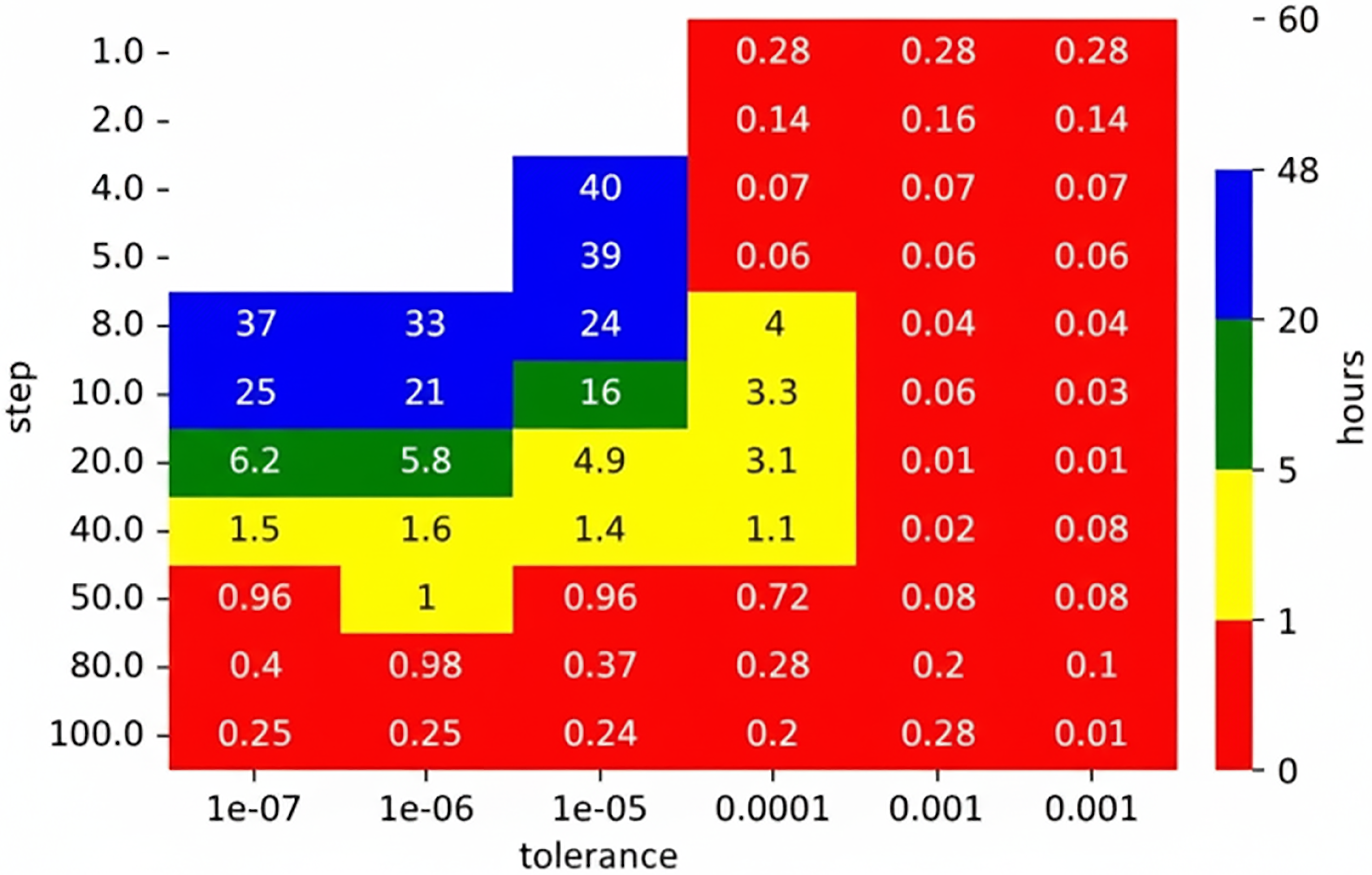
The computation time of ftaproxim for the distribution network model.

As expected, the highest value of tolerance led to the fastest computation. Higher values of the time step shortened computation time as well. However, not all the combinations led to satisfying results in terms of the correctness of the result. While the tolerance 1 × 10⁻³ leads to the fastest computation, the results are wildly unusable as there was no transition and therefore all the unavailabilities are equal to zero for 0.7 small steps. For higher steps, the changes were detected, but mainly in the central part, as can be seen in Figure 16. Similarly, the same situation to a lesser extent occurred for the tolerance 1 × 10⁻⁴ (Figure 17). For steps 1 and 2, the unavailabilities were zero; however, choosing too big a step led to nonsensical results, such as the case where step equals 100 and unavailability is 2 (Figure 18). On the other hand, choosing low values of the tolerance and high values of step seem to produce wrong values as well, such as the case where tolerance is 1 × 10⁻⁵ and step is 100 (Figure 19). There seems to exist a sweet spot for the values of tolerance and step, where the results seem plausible, that is, tolerance is 1 × 10⁻⁴ and step is 50, or tolerance is 1 × 10⁻⁶ and step is 8 (Figure 20). However, the combination of these input parameters requires a long computation time: 0.72 h and 33 h on the IT4Innovations cluster. The absolute error for the former case is 0.0001, and 0.0014 for the latter.

Figure 16.

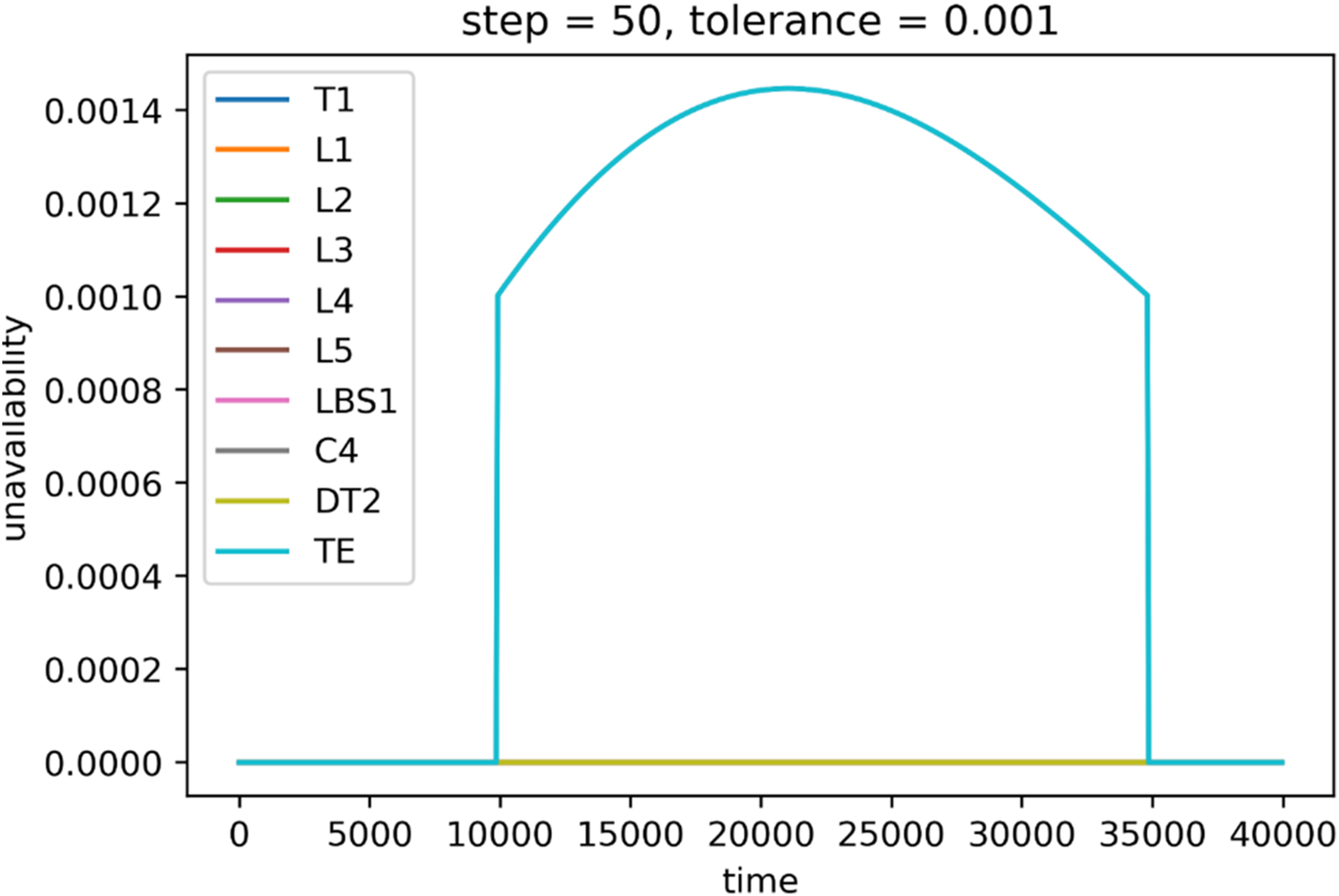
System unavailability (y-axis) during mission time (x-axis), step = 50, tolerance = 0.001.

Figure 17.

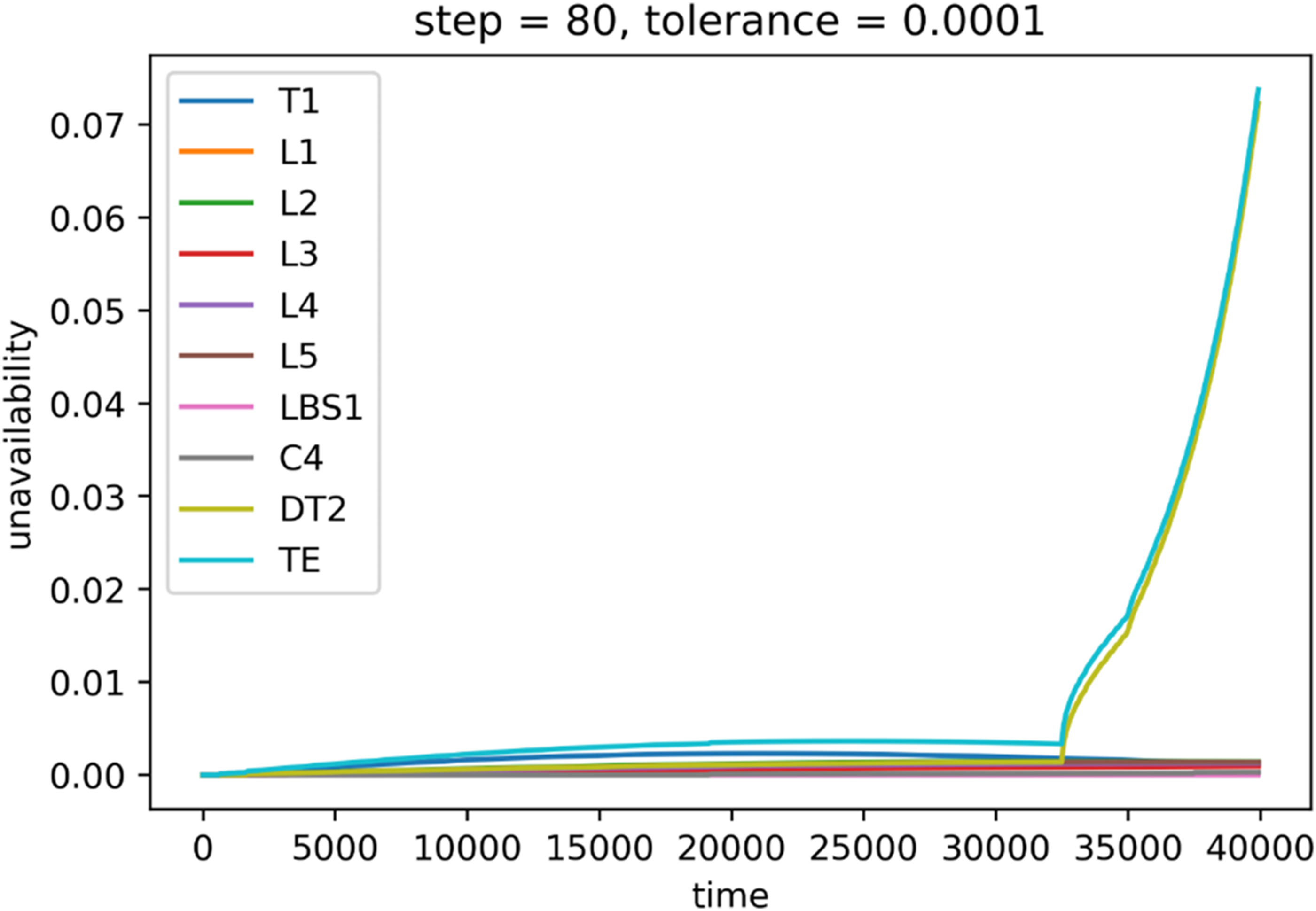
System unavailability (y-axis) during mission time (x-axis), step = 80, tolerance = 0.0001.

Figure 18.

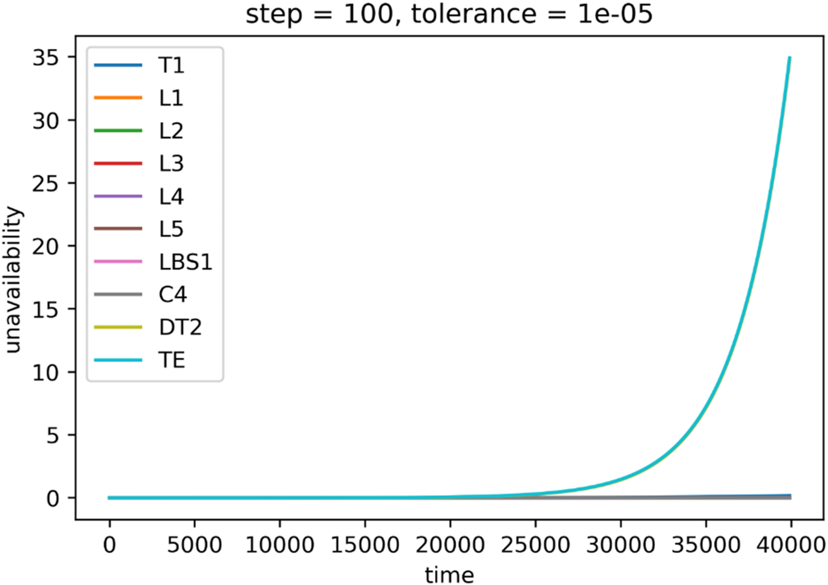
System unavailability (y-axis) during mission time (x-axis), step = 100, tolerance = 1 × 10⁻⁵.

Figure 19.

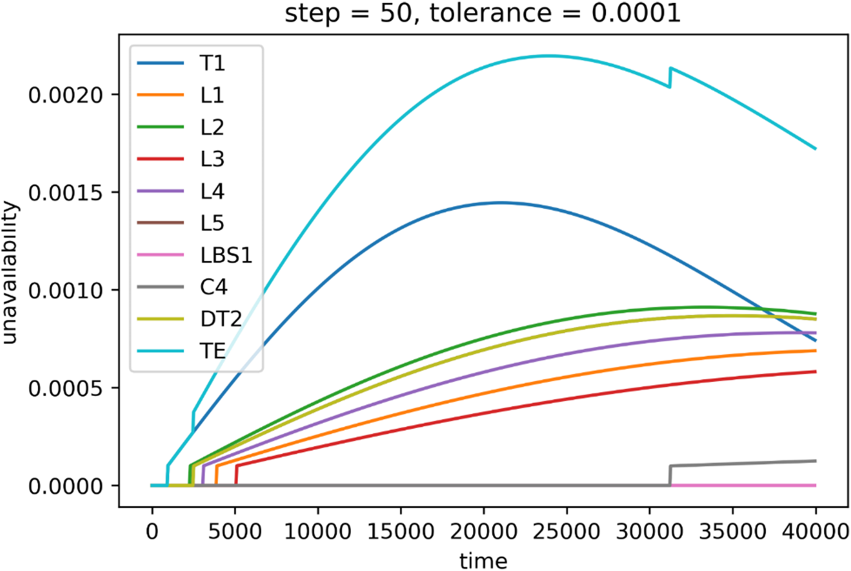
System unavailability (y-axis) during mission time (x-axis), step = 50, tolerance = 0.0001.

Figure 20.

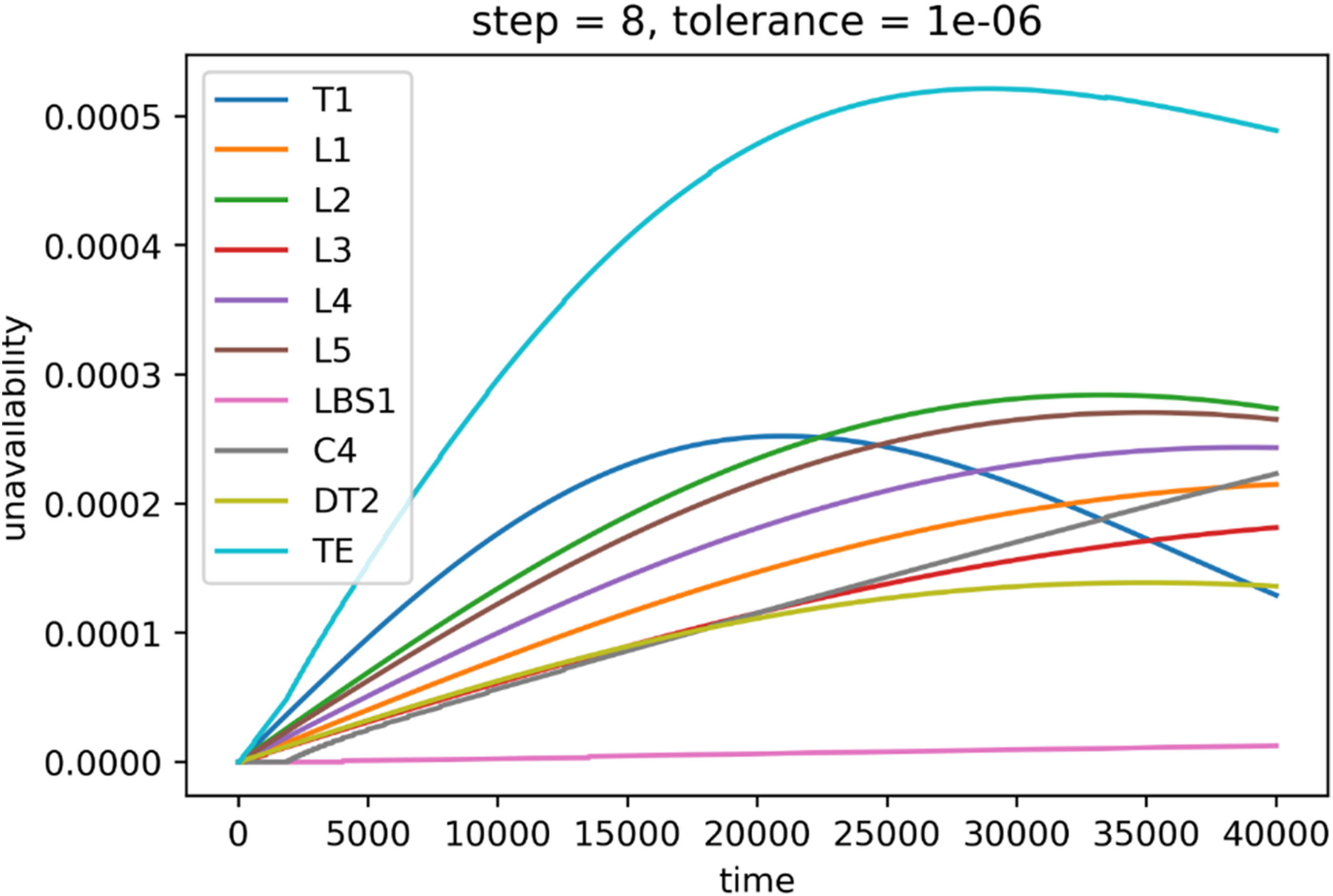
System unavailability (y-axis) during mission time (x-axis), step = 8, tolerance = 1 × 10⁻⁶.

The TE (teal line) represents the unavailability of the whole system throughout the 40,000 h mission time. However, the computation time is still too long even for the electricity network. For this reason, future research will include an open-source development and testing of an alternative computational approach for time-dependent unavailability modelling given by Briš and Byczanski (2017), which seems to be useful for supercomputers, as the algorithm can be parallelized.

Conclusions and future work

The ftaproxim package proved to be the most suitable to fulfil the set needs (an example in Appendix A is available). With the correct setting of the input tolerance and time step parameters, it can achieve similar results as an unavailability algorithm based on the commercial MATLAB software. The results showed that decreasing tolerance can significantly speed up the computational time (from 264 h to just 8 h), but the result can be very different, especially for longer mission times (error of 0.8 × 10⁻⁴ for mission time 10,000 h, versus 9.6 × 10⁻⁴ for mission time 40,000 h). Increasing the time step had a lower influence on the computational time (from 264 h to 50 h), but the result was close (error was just 1 × 10⁻⁴). Unsurprisingly, combining both approaches led to the fastest computational times (0.05 and 5 h for 10,000 and 40,000 h mission times, respectively), but what might be surprising are the quite accurate results (error 1.9 × 10⁻⁴ and 1.5 × 10⁻⁴ for 10,000 and 40,000 h mission times, respectively). Higher time steps lead to a lower number of calculations, and the decreased tolerance will not propagate into the results as much. Still, the calculation times of the ftaproxim package are a significant weakness and also an opportunity for future improvements of the results (also can be seen in Appendix B). For example, it can be assumed that with appropriate parallelization, we would achieve a significant reduction in the time required for the calculation, even while maintaining high accuracy. Also, a valid minimal cut set should be available, which cannot be easily found for larger networks.

This work addresses a critical gap in the reliability analysis of interconnected infrastructures – specifically, the lack of open, reproducible, and scalable methods for unavailability analysis of power and communication networks. While prior studies have largely relied on commercial tools with limited transparency and flexibility, this study systematically evaluates two open-source R packages, FaultTree and ftaproxim, on a real infrastructure model from the Czech Republic represented as acyclic graphs.

The theoretical contribution lies in the novel application and benchmarking of ftaproxim, a recently developed package based on proxel simulation, to model ageing components using a variety of probabilistic distributions. This contrasts with traditional tools such as FaultTree, which assume exponential failure distributions and are limited to asymptotic unavailability analysis. Our work demonstrates how ftaproxim can be tuned via tolerance and time-step parameters to balance computational efficiency and accuracy – an aspect not previously explored in the literature.

Furthermore, by deploying these tools on supercomputers (Barbora and Karolina), a reproducible and scalable framework for reliability analysis is provided, which is essential for critical infrastructure systems. The results show that the open-source approach can achieve accuracy comparable to commercial software (e.g. Matlab), with absolute errors as low as 1 × 10⁻⁴, while offering greater flexibility in modelling assumptions.

To support transparency and future research, we have included the comparative Table 2 outlining the limitations of existing methods and how our approach addresses them. Additionally, the open-source code and data used in our experiments are provided in Appendices A and B and in Electronic Appendices A and B, enabling this study to serve as a benchmark for future work in the field.

It is expected that these contributions – (1) the first systematic evaluation of ftaproxim for interconnected infrastructure, (2) the demonstration of open-source reliability analysis on HPC, and (3) the provision of reproducible benchmarks – represent a significant advancement in the scientific understanding and practical application of unavailability analysis (Briš et al., 2025).

Therefore, future research will be focused on the use of open tools that are able to efficiently find the minimal cut sets, such as the one mentioned in Tang and Dugan (2004). Additionally, alternative computational approaches for rapid unavailability estimations, as detailed in Briš and Byczanski (2017), will be tested on the supercomputers. Sensitivity analysis and machine learning techniques, as introduced in Praks et al. (2024), will be employed to identify key parameters of interconnected energy networks’ reliability models.

Supplemental Material

sj-pdf-1-eea-10.1177_01445987251377791 - Supplemental material for Evaluating the unavailability of interconnected power and communication networks with open-source tools on a petascale cluster

Supplemental material, sj-pdf-1-eea-10.1177_01445987251377791 for Evaluating the unavailability of interconnected power and communication networks with open-source tools on a petascale cluster by Michal Běloch, Pavel Praks, Renáta Praksová, Radek Fujdiak, Matěj Vrtal, Radim Briš and Dejan Brkić in Energy Exploration & Exploitation

Supplemental Material

sj-pdf-2-eea-10.1177_01445987251377791 - Supplemental material for Evaluating the unavailability of interconnected power and communication networks with open-source tools on a petascale cluster

Supplemental material, sj-pdf-2-eea-10.1177_01445987251377791 for Evaluating the unavailability of interconnected power and communication networks with open-source tools on a petascale cluster by Michal Běloch, Pavel Praks, Renáta Praksová, Radek Fujdiak, Matěj Vrtal, Radim Briš and Dejan Brkić in Energy Exploration & Exploitation

Footnotes

ORCID iDs

Michal Běloch

Pavel Praks

Renáta Praksová

Radek Fujdiak

Matěj Vrtal

Dejan Brkić

Funding

The authors disclosed receipt of the following financial support for the research, authorship, and/or publication of this article: This research was funded by the Ministry of the Interior of the Czech Republic (project No. VK01030109) in grant program ‘Open call in security research 2023–2029’. This work was also supported by the Ministry of Education, Youth and Sports of the Czech Republic through the e-INFRA CZ (ID:90254). This article has been supported by EU funds under the project ‘Increasing the resilience of power grids in the context of decarbonisation, decentralisation and sustainable socioeconomic development’, CZ.02.01.01/00/23_021/0008759, through the Operational Programme Johannes Amos Comenius. In addition, this work has been supported by the Ministry of Science, Technological Development and Innovation of the Republic of Serbia, grant number: 451-03-136/2025-03/200102.

Declaration of conflicting interests

The authors declared no potential conflicts of interest with respect to the research, authorship, and/or publication of this article.

Supplemental material

Supplemental material for this article is available online.

Appendix A

Properties of the FaultTree package (Silkworth, 2023) and an example of the script in R language for entering the structure of the tree in the FaultTree package for Transformer T1 (110/22 kV). It includes MTBF and MTTR expressed in hours, according to values from Table 1. Moreover, the ‘OR’ logical node is included to simulate the S1–T1 link of the acyclic graph of the distribution network S1 from Figure 1.

Properties of the FaultTree package: This provides an interactive and easy-to-understand visualization of the fault tree structure.

The tree structure is defined by addActive and addLogic commands.

addActive individual elements (leaves) are described by mean time to failure (MTTF) and MTTR

addLogic adds the logical node (‘AND’, ‘OR’).

For all logical nodes, FaultTree computes failure rates and asymptotic probabilities that the given node is not operating.

The FaultTree uses the binary decision diagrams (BDDs) to efficiently compute the minimal cut sets of a fault tree.

Given the asymptotic unavailability probabilities of the leaves (terminal events), BDD also computes the probability of the root event ‘The grid Off’ by Shannon’s decomposition (Rauzy, 1993).

Example of R script for entering the structure of the tree:

npgrid = ftree.make(type=‘or’, name=‘The grid’, name2=‘Off’)

# the creation of the tree

npgrid = addActive(npgrid, at = 1, mttf = 26,310.709, mttr =4.403, tag = ‘T1’, name = ‘Transformer’, name2 = ‘Off’)

# the addition of the component (directly to the top node 1, controlled by the parameter ‘at’),

npgrid = addLogic(npgrid, at = 1, type = ‘or’, name = ‘S1’, name2 = ‘Doesn’t work’)

# adds the logical node (‘or’ in this case);

min_cut_set = cutsets(npgrid)

# computes the minimal cut sets (the smallest sets of given elements that will cause the

# system to malfunction; minimal cut set)

Appendix B

Properties of the Ftaproxim package (Niloofar et al., 2022c) and an example of a script in R language for a definition of the component Transformer T1 in Ftaproxim package.

Properties of the Ftaproxim package:

A deterministic iterative method for unavailability estimation for multistate systems

Uses the minimal cut sets of the fault tree; individual elements (leaves) are described by density functions of time to failure and time to repair.

MTTF of a given Weibull component is computed as $MTTF = θ \cdot Γ (1 + 1 / β)$ , where $θ$ is a scale, $β$ is a known shape, and $Γ$ is a gamma function. As the $θ$ parameter of the distribution is unknown, we have to factor it out.

Inputs: list of the components and their failures and repair characteristics, minimal cut sets, mission time, time step, and tolerance

The output: the values of unavailabilities of each element at every time step (computed by the command FTUna)

A very versatile tool, it can work with all commonly used density functions (Weibull, exponential, uniform, and normal)

The time and space complexity of the algorithm is exponential in the number of discrete time steps (Horton, 2002).

An example of a script in the R language for a definition of the component Transformer T1, which has two states in Ftaproxim package: success (‘OK’) and failure (‘F’):

T1 = list(

states = c(‘OK’, ‘F’),

G = rbind(c(NA,1), c(1,NA)), # G is a transition matrix describing the probabilities of going from the state ‘OK’ to ‘F’ and vice versa.

dist = c(‘weibull’, ‘unif’),

# definition of pdf of time to failure and time to repair

# weibull represents the pdf of the time to failure and uniform represents the pdf of time to repair.

param = list(c(beta, T1_mttf/gamma(1 + 1/beta)), c(0, 2*T1_mttr)))

# parameters of pdfs: (shape $β$ , scale $θ$ ) for the two-parameter Weibull model

# and start and end of the interval for the uniform pdf.

References

Aslansefat

Kabir

Gheraibia

Papadopoulos

(2020) Dynamic Fault Tree Analysis. CRC Press eBooks.

Baklouti

Nguyen

Choley

, et al. (2017) Free and open source fault tree analysis tools survey. In: 2017 annual IEEE international systems conference (SysCon), Montreal, QC, Canada, 24–27 April 2017, pp. 1–8. New York: IEEE.

Baklouti

Nguyen

Mhenni

Choley

J-Y

Mlika

(2020) Dynamic fault tree generation for safety-critical systems within a systems engineering approach. IEEE Systems Journal 14(1): 1512–1522.

Briš

Byczanski

(2017) On innovative stochastic renewal process models for exact unavailability quantification of highly reliable systems. Proceedings of the Institution of Mechanical Engineers, Part O: Journal of Risk and Reliability 231(6): 617–627.

Briš

Praks

Fujdiak

Vrtal

Brkić

(2025) Maintenance optimization for unavailability enhancement of representative interconnected infrastructure based on minimum cost. Science Progress 108(3): 1–23.

Doelp

Lee

Linney

, et al. (1984) Quantitative fault tree analysis: Gate-by-gate method. Plant/Operations Progress 3(4): 227–238.

Garg

Ram

(2020) Reliability Management and Engineering. Boca Raton: CRC Press.

Hensel

Junges

Katoen

, et al. (2022) The probabilistic model checker storm. International Journal on Software Tools for Technology Transfer 24(4): 589–610.

Horton

(2002) A new paradigm for the numerical simulation of stochastic Petri nets with general firing times. In: Proceedings of the European simulation symposium, Darmstadt, Germany, 3–5 June, pp.129–136. SCS Europe. https://wwwacademiaedu/download/36633902/ess02_horton.pdf.

10.

Lazarova-Molnar

Mohamed

Shaker

(2017) Reliability modeling of cyber-physical systems: A holistic overview and challenges. In: 2017 workshop on modeling and simulation of cyber-physical energy systems (MSCPES), Pittsburgh, PA, USA, 21 April, pp.1–6. IEEE. https://doiorg/101109/mscpes2017.8064536.

11.

Morozov

Ding

Steurer

, et al. (2019) Openerrorpro: A new tool for stochastic model-based reliability and resilience analysis. In: 2019 IEEE 30th international symposium on software reliability engineering (ISSRE), pp. 303–312. IEEE. 10.1109/issre.2019.00038

12.

Nagaraju

Fiondella

Wandji

(2017) A survey of fault and attack tree modeling and analysis for cyber risk management. In: 2017 IEEE international symposium on technologies for homeland security (HST), pp. 1–6. IEEE. 10.1109/ths.2017.7943455

13.

Niloofar

Haghbin

Lazarova-Molnar

(2022a) Ftaproxim-R package for proxel-based simulation of fault trees: A case study. In: 2022 6th international conference on system reliability and safety (ICSRS), pp. 55–58. IEEE. 10.1109/ICSRS56243.2022.10067562

14.

Niloofar

Haghbin

Lazarova-Molnar

(2022b) Proxel-based simulation of fault trees in R. In: 2022 winter simulation conference (WSC), pp. 2523–2533. IEEE. 10.1109/wsc57314.2022.10015368

15.

Niloofar

Lazarova-Molnar

(2023) Data-driven extraction and analysis of repairable fault trees from time series data. Expert Systems with Applications 215: 119345.

16.

Niloofar

Lazarova-Molnar

Haghbin

(2022c) ftaproxim: fault tree analysis based on proxel simulation. R package version 0.0.1. https://CRAN.R-project.org/package=ftaproxim

17.

Pirbhulal

Gkioulos

Katsikas

(2021) A systematic literature review on RAMS analysis for critical infrastructures protection. International Journal of Critical Infrastructure Protection 33: 100427.

18.

Praks

Rasmussen

Lye

, et al. (2024) Sensitivity analysis of parameters for carbon sequestration: Symbolic regression models based on open porous media reservoir simulators predictions. Heliyon 10(22): e40044.

19.

Rauzy

(1993) New algorithms for fault trees analysis. Reliability Engineering & System Safety 40(3): 203–211.

20.

R Core Team . (2021) R: A Language and Environment for Statistical Computing. Vienna, Austria: R Foundation for Statistical Computing. https://www.R-project.org

21.

Ruijters

Stoelinga

(2015) Fault tree analysis: A survey of the state-of-the-art in modeling, analysis and tools. Computer Science Review 15: 29–62.

22.

Silkworth

(2023) FaultTree: Fault trees for risk and reliability analysis. R package version 1.0.1. https://CRAN.R-project.org/package=FaultTree

23.

Simon

Teixeira

da Costa

(2022) Availability estimation in photovoltaic generation systems using timed Petri net simulation models. International Journal of Electrical Power & Energy Systems 137: 106897.

24.

Tang

Dugan

(2004) Minimal cut set/sequence generation for dynamic fault trees. In: Annual symposium reliability and maintainability, 2004-RAMS, pp. 207–213. IEEE. 10.1109/RAMS.2004.1285449

25.

Vrtal

Fujdiak

Benedikt

, et al. (2023a) Time-dependent unavailability exploration of interconnected urban power grid and communication network. Algorithms 16(12): 561.

26.

Vrtal

Fujdiak

Benedikt

, et al. (2023b) Determination of critical parameters and interdependencies of infrastructure elements in smart grids. In: 2023 23rd International scientific conference on electric power engineering (EPE), pp. 1–6. IEEE. 10.1109/epe58302.2023.10149250

Supplementary Material

Please find the following supplemental material available below.

For Open Access articles published under a Creative Commons License, all supplemental material carries the same license as the article it is associated with.

For non-Open Access articles published, all supplemental material carries a non-exclusive license, and permission requests for re-use of supplemental material or any part of supplemental material shall be sent directly to the copyright owner as specified in the copyright notice associated with the article.

0.00 MB

0.03 MB

0.06 MB

Evaluating the unavailability of interconnected power and communication networks with open-source tools on a petascale cluster

Abstract

Keywords

Introduction

Modelling unavailability

Problem description

Literature overview

Novel method

Evaluation of unavailability modelling

Results and observations

Unavailability results for a 1 h step with tolerance 10−6 for a 10,000 h mission time

Unavailability results for a 1 h step with tolerance 10−5 for a 10,000 h mission time

Unavailability results for a 10 h step with tolerance 10−6 for 10,000 h mission time

Unavailability results for a 10 h step with tolerance 10−5 for 10,000 h mission time

Unavailability results for a 1 h step with tolerance 10−6 for 40,000 h mission time

Unavailability results for a 1 h step with tolerance 10−5 for 40,000 h mission time

Unavailability results for a 10 h step with tolerance 10−6 for 40,000 h mission time

Unavailability results for a 10 h step with tolerance 10−5 for 40,000 h mission time

Grid search of input parameters of the ftaproxim R package

Conclusions and future work

Supplemental Material

sj-pdf-1-eea-10.1177_01445987251377791 - Supplemental material for Evaluating the unavailability of interconnected power and communication networks with open-source tools on a petascale cluster

Supplemental Material

sj-pdf-2-eea-10.1177_01445987251377791 - Supplemental material for Evaluating the unavailability of interconnected power and communication networks with open-source tools on a petascale cluster

Footnotes

ORCID iDs

Funding

Declaration of conflicting interests

Supplemental material

Appendix A

Appendix B

References

Supplementary Material

Unavailability results for a 1 h step with tolerance 10⁻⁶ for a 10,000 h mission time

Unavailability results for a 1 h step with tolerance 10⁻⁵ for a 10,000 h mission time

Unavailability results for a 10 h step with tolerance 10⁻⁶ for 10,000 h mission time

Unavailability results for a 10 h step with tolerance 10⁻⁵ for 10,000 h mission time

Unavailability results for a 1 h step with tolerance 10⁻⁶ for 40,000 h mission time

Unavailability results for a 1 h step with tolerance 10⁻⁵ for 40,000 h mission time

Unavailability results for a 10 h step with tolerance 10⁻⁶ for 40,000 h mission time

Unavailability results for a 10 h step with tolerance 10⁻⁵ for 40,000 h mission time