Efficient automated detection of power quality disturbances using nonsubsampled contourlet transform & PCA-SVM

Abstract

The increasing complexity of modern power systems, driven by smart grid technologies, dispersed generation, and renewable energy sources, has made power quality (PQ) evaluation more challenging. Overuse of sensors and large data volumes further complicate accurate PQ assessment. This paper proposes a flexible signal decomposition methodology using the nonsubsampled contourlet transform (NSCT) for accurate PQ event detection. The NSCT's multiscale, multidirectional, and shift-invariant properties enable the decomposition of signals into transient and oscillatory components. High-frequency NSCT subbands are fused to extract oscillatory portions, while low-frequency subbands are averaged to detect transients. Morphological component analysis (MCA) and the split-augmented Lagrangian shrinkage algorithm (SALSA) optimize this process. Principal component analysis (PCA) is applied to the extracted features to reduce dimensionality and improve feature separability. These optimized features are used for training a multi-class support vector machine, with its parameters further optimized for enhanced classification accuracy. The proposed approach demonstrates superior frequency selectivity, adaptability, and computational efficiency, making it suitable for robust PQ disturbance identification and a wide range of signal-processing tasks.

Introduction

Motivation and background

Power quality (PQ) refers to the characteristics of the electrical power supply that affect the performance of connected electrical and electronic equipment (Ibrahim et al., 2023; Joga et al., 2024; Mahmoud et al., 2023; Yi et al., 2024). With the proliferation of electronic devices, fast control equipment, and renewable energy sources (RESs), maintaining a high-quality power supply has become increasingly important. PQ disturbances can be broadly categorized into transient and steady-state disturbances (Hoummadi et al., 2024; Shao et al., 2024). Transient disturbances are short-duration events, such as voltage sags (VSG) (momentary drops in voltage), swells (VSW) (momentary increases in voltage), interruptions (complete loss of voltage), and transients (rapid and short-term voltage variations). Steady-state disturbances are continuous issues, such as harmonics (additional frequency components on top of the fundamental frequency) and voltage fluctuations (small variations in voltage over time) (Kumar et al., 2022). The integration of RESs, such as solar and wind, introduces additional challenges to PQ due to their intermittent nature. Moreover, the simultaneous occurrence of multiple disturbances in the power system (PS) complicates detection and mitigation (Krishna Ponukumati et al., 2024; Masoum et al., 2010). The development of smart grids, incorporating advanced sensing, communication, and control technologies, aims to enhance PQ. However, to effectively improve PQ, it is crucial to accurately identify disturbances and their sources. This allows for the deployment of appropriate mitigation strategies. System operators have recognized the importance of monitoring PQ disturbances to maintain a stable and reliable power supply.

Consequently, efforts have been made to develop intelligent adaptive techniques for the automatic detection of multiple PQ disturbances. These techniques typically involve the use of advanced algorithms and machine learning approaches to PS data and identify disturbances in real-time (He et al., 2013). Diagnosing PQ disturbances often involves a multi-stage process, including signal processing, feature extraction, and classification (Montero et al., 2017; Shukla et al., 2014). Various techniques are employed at each stage to effectively identify and classify the disturbances. Commonly used signal processing methods include fast Fourier transform (FFT), discrete wavelet transform (DWT), and wavelet packet transform. Model-based parametric methods are employed to estimate the parameters of sinusoidal components in a signal. Once the signal has been processed, relevant features are extracted, such as statistical characteristics, frequency-domain information, and time-domain features. These features are then used as inputs to classifiers, such as decision tree (DT), fuzzy logic, artificial neural network, and support vector machine (SVM), to identify and categorize PQ disturbances (Abdelsalam et al., 2012; Arunadevi et al., 2024; Bracale et al., 2012).

In recent years, multimodal medical image fusion based on multiresolution decomposition has emerged as a powerful technique for extracting comprehensive information from source images of varying modalities. This method has advanced rapidly and gained widespread application in the past few decades. For instance, (Yao et al., 2016) combined medical images using WTs. Ref. (Zhang et al., 2011) fused CT and MRI using curvelet transforms, while (Biswal et al., 2009) developed a contourlet transform (CT)-based fusion technique for multimodal medical imaging. Ref. (Cen et al., 2023) fused MRI and SPECT using the nonsubsampled contourlet transform (NSCT). The NSCT, introduced by Biswal et al., 2014), is a well-known multiscale decomposition method that has been successfully used in applications such as image denoising, and image augmentation (Liu et al., 2015). The NSCT offers unique advantages, including its multiscale, multidirectional, and shift-invariance properties. These features allow it to capture higher dimensional singularities, such as edges and contours, which are inadequately represented by wavelets. Additionally, NSCT avoids the pseudo-Gibbs phenomena that arise in the contourlet transform. As a result, NSCT is particularly beneficial for image fusion, as it captures correlations between distinct subbands and improves the overall fusion process (Hu et al., 2008). While NSCT-based image fusion algorithms have demonstrated strong performance in the medical domain, current approaches often overlook the inter- and intra-scale dependencies of the decomposition coefficients. These relationships are important, as the features exhibit large tails and non-Gaussian distributions, which can significantly affect the fusion efficiency. Maximizing the statistical correlations between the subband coefficients can greatly enhance the performance of the fusion process (Thirumala et al., 2018).

Ref. (Hajian and Akbari Foroud, 2014) collectively explain how multiscale, multidirectional, and shift-invariant properties of the NSCT can be used to improve the extraction of features from complex datasets, such as those encountered in PQ analysis. These properties allow for a more detailed representation of the disturbances, which is essential for their accurate detection and classification. Specifically, references like (Li et al., 2013; Tahir et al., 2023) highlight the importance of maximizing statistical correlations between subband coefficients, which can significantly improve feature extraction efficiency and classification accuracy. Additionally, the ability of NSCT to handle noisy data, isolate important features, and avoid distortions caused by misregistration makes it a powerful tool for PQ monitoring, especially in real-time applications where high-frequency sampling and large datasets are common.

Research gap

A major research gap in the current literature on PQ disturbance detection and classification lies in the underutilization of advanced multiscale and multidirectional decomposition techniques, such as the NSCT, which can better capture the complex and localized features of PQ disturbances. Most existing approaches fail to fully exploit the inter- and intra-scale dependencies of decomposition coefficients, which are crucial for enhancing feature extraction, especially in the presence of non-Gaussian distributions and large-tailed features common in PQ signals. Furthermore, while various signal processing methods, such as wavelets and Fourier transforms, are widely used for PQ analysis, they often struggle with the high-dimensional and noisy nature of real-world PSs, particularly in dynamic grid environments. Additionally, the integration of machine learning techniques, including SVM, with advanced decomposition methods is still in its nascent stages, and there is limited research on optimizing the combination of these techniques to handle large-scale datasets efficiently. Addressing these gaps by incorporating NSCT and refining feature extraction methods, as well as enhancing the scalability of machine learning models, could significantly improve the accuracy and robustness of PQ disturbance detection in complex, real-time grid conditions.

Major contribution

The major contribution of this work lies in the integration of the NSCT with SVM for the classification of PQ disturbances. By leveraging the multiscale, multidirectional, and shift-invariant properties of NSCT, this approach captures finer details and localized features of PQ disturbances that traditional methods, such as wavelet transforms, often overlook. This allows for improved feature extraction, particularly for complex disturbances such as VSG, VSW, and transients, which are characterized by non-Gaussian distributions and large tails. Additionally, this method addresses the inter- and intra-scale dependencies of the decomposition coefficients, optimizing the extraction of features that are more statistically significant for classification tasks.

Another significant contribution is the application of principal component analysis (PCA) to reduce the dimensionality of the extracted features before they are fed into the SVM classifier. PCA helps to eliminate redundant or less informative features, thus improving the efficiency and accuracy of the classification process. This dimensionality reduction enhances the SVM's ability to effectively classify PQ disturbances by focusing on the most relevant features while reducing computational complexity. Furthermore, the research explores optimization strategies for SVM classifiers, including kernel selection and feature scaling, to enhance their performance. By combining NSCT with PCA and SVM, this work provides a powerful and scalable framework for real-time, accurate PQ disturbance classification in modern PSs, especially as they integrate RESs and become more complex.

NSCT-based signal decomposition technique

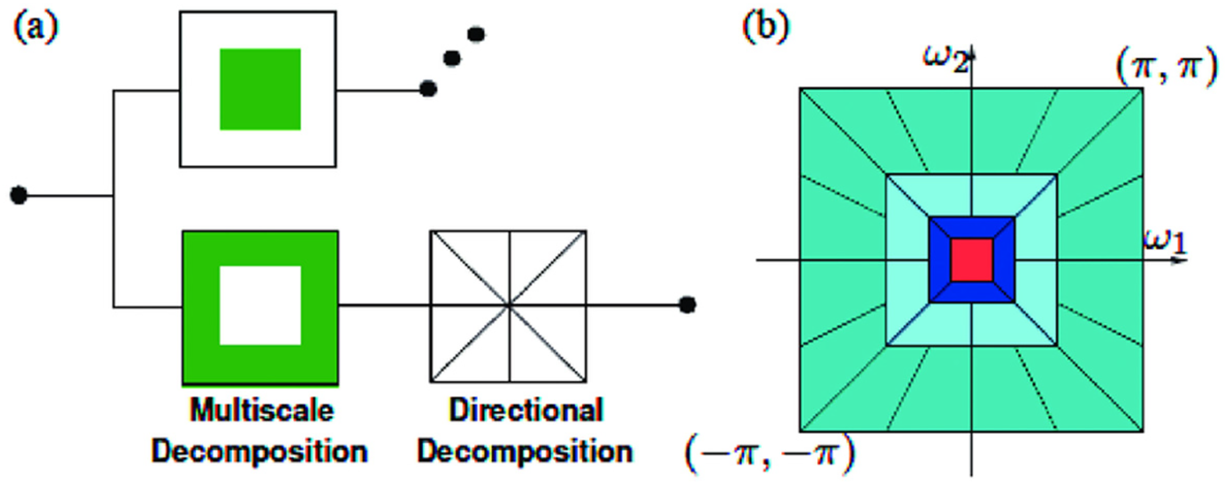
NSCT is a shift-invariant contourlet overcomplete transform with flexible multiscale, multidirectional picture expansion (Li et al., 2013). The nonsubsampled pyramids (NSP) and directional filter bank (NSDFB) stages make up the NSCT decomposition process. The former decomposes multiscale, whereas the latter decomposes directionally. Each level of the NSP separates pictures into low- and high-frequency subbands. NSP generates k + 1 sub-band pictures, one low-frequency and k high-frequency, with a decomposition level of k. NSDFB decomposes NSP high-frequency subbands at each level.

For a given subband, l decomposition directions provide 2 l directional subbands with the same size as the original picture. After repeatedly decomposing the low-frequency component, an image is divided into one low-frequency sub-signal and a sequence of high-frequency directional sub-band signal turns (k j = 1 2lj), where lj is the number of decomposition directions at the j scale. Figure 1 represents the pyramid structure of NCT (Li et al., 2013).

Figure 1.

Block diagram of NSCT of an input signal x[n].

The NCT decomposes an input signal into subbands using a series of low-pass and high-pass filters. Each level of decomposition splits the signal into two subbands: the low-pass subband captures lower frequencies, while the high-pass subband retains higher frequencies or details. By recursively applying the NCT up to the desired level, a multilevel signal representation is achieved. Constraints on the scale (α) and shape (β) parameters, along with proper filter design, ensure accurate decomposition and reconstruction while preserving the signal's characteristics without redundancy.

The NSP, constructed through iterated nonsubsampled filter banks, achieves multiscale decomposition by representing signals at multiple resolutions. The ideal frequency response of the nonsubsampled pyramid, shown in Figure 1, ensures that details at different scales are effectively captured. This construction process involves cascading nonsubsampled filter banks, where each subsequent level of decomposition uses filters upsampled by a factor of 2 in both dimensions. This upsampling allows finer-scale information to be captured efficiently, employing the ‘à trous’ algorithm, a wavelet decomposition technique. Cascading is performed by connecting the output of one analysis block to the input of the next, enabling multiscale decomposition through iterative filtering. The equivalent filters used for k-th level cascading in the nonsubsampled pyramid are critical for ensuring perfect reconstruction, where the reconstructed signal closely matches the original.

Investigations on the proposed signal processing technique

The proposed method integrates the NSCT with SVM for the effective detection and classification of PQ disturbances. This method leverages the NSCT's ability to capture detailed features from the PS signals, and the classification strength of SVM to accurately categorize disturbances like voltage sags, swells, harmonics, and transients. The approach is designed to improve the accuracy and efficiency of PQ disturbance classification in complex PS. The first step in the proposed method is signal preprocessing, where raw PS data is cleaned by removing noise and irrelevant components. Preprocessing techniques such as bandpass filtering and normalization are employed to prepare the signal for further analysis. This step ensures that only the essential parts of the signal, free from noise, are analyzed, which is crucial for accurate feature extraction. Following the preprocessing, the signal is subjected to feature extraction using the NSCT.

The NSCT is a multiresolution, multidirectional, and shift-invariant method that decomposes the signal into multiple frequency subbands. Unlike traditional transforms, NSCT captures finer details and edges within the signal, making it particularly useful for detecting subtle disturbances in PQ data. By providing a shift-invariant decomposition, NSCT can handle non-stationary and complex signals commonly encountered in PQ monitoring. The subbands obtained from NSCT are then used to extract features that represent key characteristics of the disturbances. Since NSCT generates a large number of features, dimensionality reduction is necessary to make the data manageable. The PCA is applied to reduce the number of features while retaining the variance of the data. PCA identifies the most significant features by transforming the data into a smaller set of components. This process not only reduces the computational load but also enhances the performance of the classification algorithm by eliminating redundant and irrelevant features. Once the features are extracted and reduced in dimensionality, they are fed into an SVM classifier for categorization. SVM is a powerful supervised machine learning algorithm known for its effectiveness in high-dimensional spaces. It works by finding an optimal hyperplane that separates the different classes of PQ disturbances. In this method, SVM is trained using the features derived from the NSCT and PCA steps, enabling it to classify disturbances such as voltage sags, swells, harmonics, and transients accurately. To improve the performance of the SVM classifier, optimization techniques are applied. These techniques include selecting the best kernel type (linear, polynomial, or radial basis function), scaling the features to a comparable range, and applying regularization to prevent overfitting. These optimizations ensure that the SVM classifier can handle a variety of disturbance types and generalize well to unseen data.

Finally, the proposed method is designed to be scalable and suitable for real-time implementation in large-scale power grids. With the increasing amount of data generated by distributed sensors, the method incorporates strategies for efficient computation. Distributed and parallel computing frameworks can be utilized to manage the computational demands of the NSCT and SVM processes, while edge computing at sensor nodes can reduce the load on centralized systems by enabling localized pre-processing and denoising. These techniques ensure that the method can handle large datasets with high-frequency sampling and deliver real-time disturbance detection and classification.

NSCT method

The NSCT consists of two main components: the NSP and the NSDFB. These components work together to achieve multiscale and directional decomposition of signals. The NSP performs the multiscale decomposition by dividing the signal into low-frequency and high-frequency subbands. Specifically, at the k-th decomposition level, the NSP produces a total of k + 1 subbands: one low-frequency subband and k high-frequency subbands. This process helps break down the signal at different scales, allowing for a detailed representation of both coarse and fine details (Kim et al., 2023).

In the next stage of the NSCT, the high-frequency subbands generated by the NSP are further decomposed using the NSDFB. The NSDFB applies directional decomposition, where the signal is divided into multiple directional subbands. If l represents the number of directions chosen for the decomposition, then 2 l directional subbands are obtained. These directional subbands maintain the same size as the original signal, preserving key information while allowing for the detailed analysis of edges and contours. The process of decomposition continues iteratively, where each low-frequency subband undergoes further decomposition, resulting in additional high-frequency directional subbands. The final result is a set of directional subbands that represent the signal at different scales and orientations. The correlation coefficients of the variables in the NSCT coefficients show significant correlations that are different from zero, as illustrated in Figure 1. These correlations reflect the interdependence between the different decomposition levels and directions. To model these relationships, a generalized Gaussian distribution (GGD) is applied to approximate the distribution of the NSCT subband coefficients. The GGD is characterized by two parameters: the shape parameter (β) and the scale parameter (γ). The shape parameter controls the overall shape of the distribution, while the scale parameter adjusts the spread. The GGD model is capable of representing a wide range of distribution types, from super-Gaussian (heavy-tailed) to sub-Gaussian (light-tailed) distributions. This flexibility makes the GGD a useful tool for modeling the complex distributions of NSCT coefficients in PQ disturbance analysis. By adjusting the parameters β and γ, the GGD model can be tailored to fit the observed data, improving the accuracy of the signal analysis (Kim et al., 2023; Li et al., 2016).

$$P(x;\alpha ,\beta )={\displaystyle \frac{\beta }{2\alpha I\left({\displaystyle \frac{I}{\beta }}\right)}{e}^{-{\left(\frac{|x|}{\alpha }\right)}^{\beta }}}$$

(1)

where $I^{\mathrm{\prime }}(\cdot )$ is the Gamma function, $\alpha$ is the scale parameter (width of the PDF peak), and $\beta$ is the shape parameter which tunes the decay rate of the density function. In this context, the parameters α and β are computed using the maximum likelihood (ML) estimator. This estimator finds the values of α and β that maximize the likelihood function based on the observed data.

$$L(x;\alpha ,\beta )=\log \prod _{i=1}^{n}p(x_i;\alpha ,\beta )$$

(2)

In this case, $\alpha$ and $\beta$ are parameters that need to be estimated. We can obtain the unique root by the likelihood equations below; here $\mathrm{\Psi }(\cdot )$ denotes the digamma function:

$${\displaystyle \frac{\mathrm{\partial }L(x;\alpha ,\beta )}{\mathrm{\partial }\beta }={\displaystyle \frac{L}{\alpha }+\sum _{i=1}^N{\displaystyle \frac{\beta {|x_i|}^{\beta }{\alpha }^{-\beta }}{\alpha }=0}}}$$

(3)

$${\displaystyle \frac{\mathrm{\partial }L(x;\alpha ,\beta )}{\mathrm{\partial }\beta }={\displaystyle \frac{L}{\beta }+{\displaystyle \frac{L\mathrm{\Psi }\left({\displaystyle \frac{1}{\beta }}\right)}{{\beta }^2}-\sum _{i=1}^N{\left({\displaystyle \frac{|x_i|}{\alpha }}\right)}^{\beta }\log \left({\displaystyle \frac{|x_i|}{\alpha }}\right)=0}}}$$

(4)

Let $\beta$ be fixed and $\beta >$ 0; then equation (4) has the unique solution, which is the real and positive value:

$$\hat{\alpha }={\left({\displaystyle \frac{\beta }{N}\sum _{i=1}^N{|x_i|}^{\beta }}\right)}^{\frac{1}{\hat{\beta }}}$$

(5)

Combining equations (4) and (5), the shape parameter ft can be solved by the following transcendental equation:

$$1+{\displaystyle \frac{\mathrm{\Psi }\left({\displaystyle \frac{1}{\hat{\beta }}}\right)}{\hat{\beta }}-{\displaystyle \frac{{\sum }_{i=1}^N{|x_i|}^{\hat{\beta }}\log |x_i|}{\sum {|x_i|}^{\hat{\beta }}}+{\displaystyle \frac{\log (\left({\displaystyle \frac{\hat{\beta }}{N}}\right){\sum }_{i=1}^N{|x_i|}^{\hat{\beta }}}{\hat{\beta }}=0}}}$$

(6)

In (6), the determination $\hat{\beta }$ can be effectively solved using the Newton–Raphson iterative procedure (Li et al., 2013) and the algorithm was described in (Ozgonenel et al., 2013). Therefore, with only two parameters, we can accurately characterize the marginal distribution of the NSCT coefficients. The Dependency of Different NSCT Subbands: the Kullback–Leibler Divergence (KLD) is a way to measure the difference between two probability distributions. The KLD is a concept often used in information theory and statistics to quantify how one distribution differs from another. The KLD is often denoted as D_KL (P || Q), where P and Q are the two distributions being compared. Here P is represented by a probability density function (PDF) which is denoted as p (X; θ₂) parameterized by θ₂, and Q is represented by a PDF denoted as p (X; θ₂) parameterized by θ₂.

Fusion of high-frequency coefficients for enhanced signal representation

The high-frequency subbands of a signal typically contain critical information regarding noise, harmonics, or distortion, which are essential for accurate signal analysis (Li et al., 2013; Singh et al., 2023). In many applications, different signal modalities provide overlapping and unique insights into the same subject or scene. To effectively combine these diverse pieces of information, a selection rule is implemented to prioritize and capture the most significant features of the source signal for fusion.

This fusion method focuses on high-frequency subbands and introduces the concept of weight maps to guide the process. Weight maps assign importance to different coefficients based on their relevance to the overall signal, ensuring that the fusion process emphasizes the most critical components. Due to the multiscale and multidirectional characteristics of NSCT coefficients, there are inherent dependencies between high-frequency coefficients across different subbands. These dependencies are utilized to update and enhance the coefficients, ensuring a more accurate representation of the original signal.

The process involves updating the high-frequency coefficients by leveraging the relationships between them across NSCT subbands. Once updated, these coefficients are combined according to the weight maps, which control the fusion process by emphasizing important subbands. The goal is to enhance the fused signal, capturing fine details while preserving the overall complexity. However, the success of this method depends on the specific implementation of the fusion rule and the parameters chosen. A balanced approach is sought to maintain the integrity of critical features while minimizing the introduction of artifacts. The method's effectiveness will vary depending on the nature of the source signal and the specific fusion task at hand (Li et al., 2013; Singh et al., 2023).

Computing the regional standard deviation $D_{\lambda }(x,y)$

$$D_{\lambda }(x,y)=\sqrt{\sum _{mϵM,nϵN}\omega (m,n)\times {[C_{\lambda }(x+m,y+n)-S_{\lambda }(x,y)]}^2}$$

(7)

1. Calculating the normalized Shannon entropy (Li et al., 2013; Singh et al., 2023).

   $$E_{\lambda }(x,y)={\displaystyle \frac{1}{|R|}\sum _{i.j}(C_0^{\lambda }(i,j){)}^2\log (C_0^{\lambda }(i,j){)}^2}$$

   (8)

2. Computing the weights $({\delta }_{\lambda },{\xi }_{\lambda })$ of the standard deviation $D_{\lambda }(x,y)$ and the information entropy $E_{\lambda }(x,y)$ , respectively.

   $${\delta }_{\lambda }={\displaystyle \frac{{|D_{\lambda }(x,y)|}^{\alpha }}{{|D_A(x,y)|}^{\alpha }+{|D_B(x,y)|}^{\alpha }};{\xi }_{\lambda }={\displaystyle \frac{E_{\lambda }(x,y)}{E_A(x,y)+E_B(x,y)},}}$$

   (9)

3. Fusion for low-frequency

Let $C_0^{\lambda }(x,y)$ denote the low-frequency subband coefficient at location $(x,y)$ ; $\lambda$ is input image A, B. Finally, the fused image can be obtained by (Li et al., 2013; Singh et al., 2023).

$$C_0^{\lambda }(x,y)=\sum _{\lambda =A,B}[{\delta }_{\lambda }{C}_0^{\lambda }(x,y)+{\xi }_{\lambda }{C}_0^{\lambda }(x,y)]$$

(10)

High-frequency subbands capture detailed information like edges, lines, and corners. The goal of this process is to capture salient information from different imaging modalities and enhance the overall fusion performance. Updating of the High Frequency Subband Coefficients. First, we calculate the horizontal dependency ${\mathrm{jsd}}_{\mathrm{l},\theta ,\mathrm{h}}$ between coefficients with different directions at the same scale $\mathrm{l}$ as

$$js{d}_{l,\theta ,h}(x,y)=\sum _{j=1.j\mathrm{\&}num;i}^K{D}_{JS}(C_{l,{\theta }_i}(x,y),C_{l,{\theta }_j}(x,y)),$$

(11)

where K is the total of the subbands at the l th scale.

Then we calculate the vertical dependency $js{d}_{i,\theta ,v}$ between the specified subband's (for instance subband $i$ ) parents and children

$${\mathrm{jsd}}_{\mathrm{l},\theta ,\mathrm{v}}(\mathrm{x},\mathrm{y})=\sum _{\mathrm{j}=1}^{\mathrm{K}}{\mathrm{D}}_{\mathrm{JS}}({\mathrm{C}}_{\mathrm{l},{\theta }_{\mathrm{i}}}(\mathrm{x},\mathrm{y}),{\mathrm{C}}_{\mathrm{l}-1,{\theta }_{\mathrm{j}}}(\mathrm{x},\mathrm{y}))+{\mathrm{D}}_{\mathrm{JS}}({\mathrm{C}}_{\mathrm{l},{\theta }_{\mathrm{i}}}(\mathrm{x},\mathrm{y}),{\mathrm{C}}_{\mathrm{l}+1,{\theta }_{\mathrm{j}}}(\mathrm{x},\mathrm{y}))$$

(12)

Further, the horizontal and vertical dependency components are normalized, respectively,

$$js{d}_{l,\theta ,h}(x,y)={\displaystyle \frac{js{d}_{l,\theta ,h}(x,y)}{js{d}_{l,\theta ,h}(x,y)+js{d}_{l,\theta ,v}(x,y)},js{d}_{l,\theta ,v}(x,y)={\displaystyle \frac{js{d}_{l,\theta ,v}(x,y)}{js{d}_{l,\theta ,h}(x,y)+js{d}_{l,\theta ,v}(x,y)}}}$$

(13)

Finally, the high-frequency NSCT coefficients are revised as

$$C_{l,\theta }(x,y)=C_{l,\theta }(x,y)\sqrt{1+js{d}_{l,\theta ,h}{(x,y)}^2+js{d}_{l,\theta ,v}{(x,y)}^2}$$

(14)

The process of constructing weight maps using saliency information and applying a Gaussian filter to each high-pass subband. These weight maps play a crucial role in guiding the fusion algorithm for achieving an informative and balanced fused signal. By assigning appropriate weights to different parts of the subband coefficients based on their saliency levels, the fusion process is enhanced and prioritizes significant elements such as edges and corners.

$$S_{l,\theta }(x,y)=|C_{l,\theta }(x,y)|*g_{r_g,{\theta }_g}(x,y)$$

(15)

where $g(\cdot )$ is a Gaussian low pass filter, whose size is $(2r_g+1)\times (2r_g+1)$ , and the parameters $r_g$ and ${\theta }_g$ are set to 5. Next, the weight maps are determined by comparison of the saliency maps $(S_{l,\theta }^n(x,y),nϵ[A,B])$

$$W_{l,\theta }^n(x,y)=\{\begin{array}{c}1\\ 0\end{array}\begin{array}{c}if(S_{l,\theta }^n(x,y)=max(S_{l,\theta }^A(x,y),S_{l,\theta }^B(x,y))\\ \mathrm{otherwise}\end{array}$$

(16)

Finally, the fused subband coefficients $C_{l,\theta }^F(x,y)$ can be obtained by the weighted summation

$$C_{l,\theta }^F(x,y)=W_{l,\theta }^A(x,y)C_{l,\theta }^A(x,y)+W_{l,\theta }^B(x,y)C_{l,\theta }^B(x,y)$$

(17)

• Determination of energy to capture the features

The challenges associated with evaluating the sparsity of wavelet coefficients obtained through the NSCT decomposition. Unlike traditional WTs, NSCT employs a two-channel bandpass filter for iterative signal decomposition, resulting in a sequence of wavelet coefficients that can vary in length. This poses difficulties when using traditional measures like Shannon entropy to evaluate sparsity accurately. The value is called “SAEWSE” to address this issue (Li et al., 2013; Singh et al., 2023).

$$p_i^{(j)}={\displaystyle \frac{E_{\lambda }(x,y)/\mathrm{Nj}|\mathrm{w}(\mathrm{j})}{{\sum }_{j=1}^{j+1}{\sum }_{i=1}^{N_j}{\displaystyle \frac{E_j}{N_j}|w_i^j|}}}$$

(18)

$$\mathrm{SAEWSE}=-\sum _{j=1}^{J+1}\sum _{i=1}^{N_j}{p}_i^{(j)}ln{p}_i^{(j)}$$

(19)

where Ej, Nj, and w(j) I represent the NSCT energy which is represented in equation (11), length of the sequence, and coefficients of wavelets respectively up to the jth layer. To address this challenge, it appears that a different measure called “SAEWSE” (sub-band average energy-weighted wavelet Shannon entropy) is introduced.

This measure might be designed specifically to evaluate the sparsity of NSCT coefficients in a way that accounts for their unique properties and the variations caused by the decomposition process.

$$Y=[Y(JLS,N),Y2(2,N),\cdot \cdot \cdot Y(JHS,N)]T\in R(JHS-JLS+1)\times N$$

(20)

$$EY(J,N)=||HILBERT(Y(J,N))||2,JLS\le J\le JHS$$

(21)

We acquire the frequency domain sequence FE(j,) by performing the M-point discrete Fourier transform (DFT) on Ey(j, n), and from this, we can derive the power spectrum P_E(j,) of the layer j signal envelope.

$$P_E(j,\omega )={\displaystyle \frac{F_E(j,w).F_E*(j,w)}{M}}$$

(22)

In this case, the Power Spectrum Kurtosis (PSK) is defined as the complex conjugate of the power spectrum (F_E*(j, ω)).

$$PSK(j)={\displaystyle \frac{{\displaystyle \frac{1}{M/2}{\sum }_{i=1}^{M/2}{[P_E(j,w)-\overline{P_E(j,w)}]}^4}}{{\left[{\displaystyle \frac{1}{M/2}{\sum }_{i=1}^{M/2}{[P_E(j,w)-\overline{P_E(j,w)}]}^2}\right]}^2}}$$

(23)

Based on Figure 2, it is observed that the value of SAEWAE (presumably an evaluation metric) is the lowest among the presented options with respect to GCD and JSD.

Figure 2.

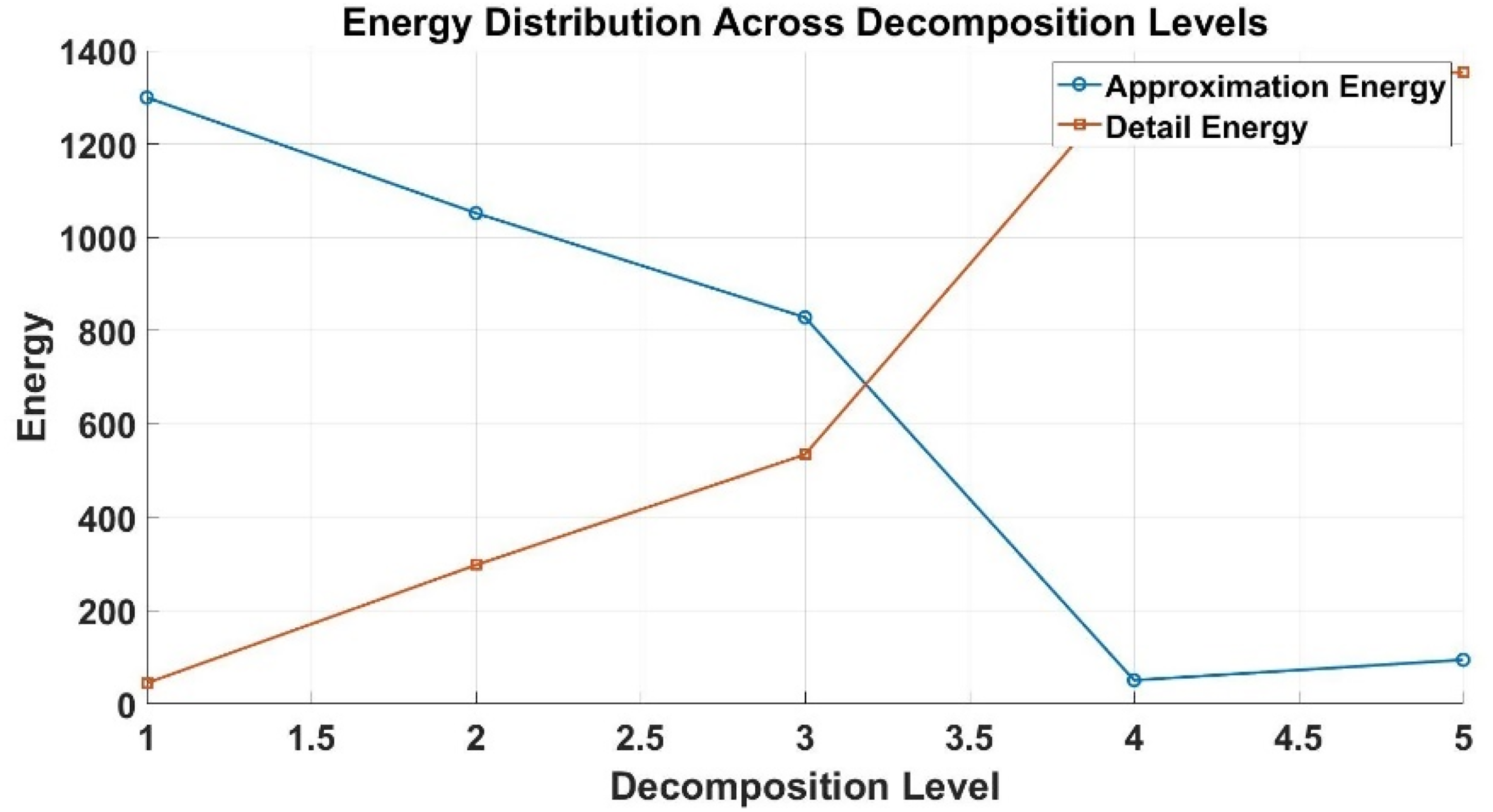
A plot illustrating the approximation and detail energy values at each decomposition level, highlighting the energy redistribution as decomposition progresses.

Figure 2 shows how energy is distributed between the approximation and detail components across different decomposition levels. The approximation energy captures the low-frequency content, while the detail energy represents high-frequency components such as disturbances and noise. At Level 3, a significant drop in approximation energy is observed, accompanied by a substantial rise in detail energy. This indicates that critical high-frequency information, essential for distinguishing PQ disturbances, is concentrated at this level. Hence, Level 3 is chosen as the optimal decomposition level to strike a balance between preserving meaningful features and avoiding over-decomposition, which could introduce redundancy and increase computational load.

Parameters selection

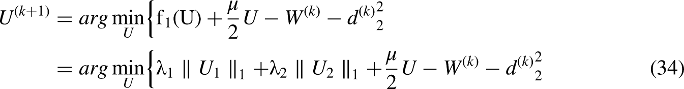
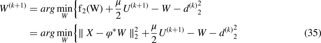
This study presents a technique to decompose a signal into its oscillatory and transient components. To achieve this, sparse representations of these components are obtained by using the parameters δλ and ξλ in the NSCT. The oscillatory component is represented by high δλ and ξλ values in NCT, whereas the transient component is modeled with low δλ and ξλ values. The separation of these components is effectively facilitated by morphological component analysis (MCA), which leverages the limited coherence between the low and high values of δλ and ξλ. To address the optimization problem inherent in MCA, the split-augmented Lagrangian shrinkage algorithm (SALSA) (Singh et al., 2023) is employed in this study. This method iteratively updates the oscillatory and transient components, facilitating the efficient decomposition of the signal. The ability of the NCT to encode distinct frequency and temporal characteristics across different subbands enhances the overall representation of the signal components (Biswal et al., 2009; Zhang et al., 2011).

The parameter selection process is key to achieving a balance between computational efficiency and the accuracy of the decomposition. By fine-tuning the values of δλ and ξλ, the desired frequency decomposition can be accurately achieved. This enables the separation of oscillatory and transient features, capturing the full complexity of the signal for more effective analysis. If X is the signal, then a signal is divided into high and low oscillatory components. The objective of MCA is to find out X₁ and X₂ separately. Where X₁ and X₂ are the sparse representation of the matrix. X₁ is sparsely represented by NCT₁ with JSD. The transformation matrix is denoted by φ₁. Similarly, X₂ is sparsely represented by NCT₂ with parameters of different JSD. A transformation matrix is denoted by φ₂ (Biswal et al., 2009; Zhang et al., 2011).

$$\mathrm{X}={\mathrm{X}}_1+{\mathrm{X}}_2$$

(24)

$$\{{\mathrm{W}}_1^{\mathrm{opt}},{\mathrm{W}}_2^{\mathrm{opt}}\}=\underset{{\mathrm{w}}_1}{\arg }\underset{{\mathrm{w}}_2}{\min }\parallel W_1{\parallel }_1+\parallel W_2{\parallel }_1$$

Such that

$$X={\varphi }_1*W_1+{\varphi }_2*W_2$$

(25)

where $W_1,$ represents the Calculation of the NCT1 coefficients of the signal ${\mathrm{X}}_1$ .where $W_2$ represents the calculation of the NCT2 coefficients of the signal ${\mathrm{X}}_2$ .

$$\{W_1^{opt},W_2^{opt}\}=\underset{w_1}{arg}\underset{w_2}{\min }\parallel W_1{\parallel }_1+\parallel W_2{\parallel }_1\parallel X-{\varphi }_{*}^1{W}_1-{\varphi }_{*}^2{W}_2{\parallel }_2\le \mathit{\epsilon }$$

(26)

$$\{W_1^{opt},W_2^{opt}\}=\underset{w_1}{arg}\underset{w_2}{\min }\parallel X-{\phi }_1*W_1-{\phi }_2*W_2{\parallel }_2^2+{\lambda }_1\parallel W_1{\parallel }_1+{\lambda }_2\parallel W_2{\parallel }_1$$

(27)

Using optimal coefficient vector ${\mathrm{W}}_1^{\mathrm{opt}},{\mathrm{W}}_2^{\mathrm{opt}}$ the component X₁ and X₂ can be calculated.

$$J(W_1,W_2)=\parallel X-{\phi }_1*W_1-{\phi }_2*W_2{\parallel }_2^2+{\lambda }_1\parallel W_1{\parallel }_1+{\lambda }_2\parallel W_2{\parallel }_1$$

(28)

Here λ₁ and λ₂ are the Lagrangian Multipliers

$${\lambda }_1(k)={\theta }_1\parallel {\psi }_1^{(k)}{\parallel }_2{\lambda }_1(k)={\theta }_2\parallel {\psi }_2^{(k)}{\parallel }_2$$

(29)

The objective of minimizing the function in signal decomposition with sparsity constraints is crucial for achieving effective signal analysis (Biswal et al., 2009; Zhang et al., 2011). To address these challenges, the SALSA is employed, a specialized optimization method designed to efficiently solve non-smooth and constrained optimization problems. SALSA's iterative updating of variables while considering constraints makes it well-suited for tackling these complex problems. The core principle of SALSA revolves around the following minimization problem. The generic formulation of the unbounded optimization issue, as described in equation (14), is (Biswal et al., 2009; Zhang et al., 2011):

$$\underset{\mathrm{w}}{\min }\{{\mathrm{f}}_1(\mathrm{W})+{\mathrm{f}}_2(\mathrm{W})\}$$

(30)

where

$${\mathrm{f}}_1(\mathrm{W})={\lambda }_1\parallel W_1{\parallel }_1+{\lambda }_2\parallel W_2{\parallel }_1$$

(31)

$${\mathrm{f}}_2(\mathrm{W})=\parallel X-\phi *W{\parallel }_2^2$$

(32)

where

$$\phi *={\phi }_1*,{\phi }_2*andW=\left[\begin{array}{c}{W}_1\\ W_2\end{array}\right]\underset{W,U}{min}\{{\mathrm{f}}_1(\mathrm{U})+{\mathrm{f}}_2(\mathrm{W})\}$$

(33)

Such that U = W, where U =  $\left[\begin{array}{c}{U}_1\\ U_2\end{array}\right]$ is used and ${\phi }_1*,{\phi }_2*$ are the azimuth and elevation angles, respectively.

$$U^{(k+1)}=arg\underset{U}{min}\{{\mathrm{f}}_1(\mathrm{U})+{\displaystyle \frac{\mu }{2}U-W^{(k)}-{d^{(k)}}_2^2}=arg\underset{U}{min}\{{\lambda }_1\parallel U_1{\parallel }_1+{\lambda }_2\parallel U_2{\parallel }_1+{\displaystyle \frac{\mu }{2}U-W^{(k)}-{d^{(k)}}_2^2}$$

(34)

$$W^{(k+1)}=arg\underset{W}{min}\{{\mathrm{f}}_2(\mathrm{W})+{\displaystyle \frac{\mu }{2}{U}^{(k+1)}-W-{d^{(k)}}_2^2}=arg\underset{W}{min}\{\parallel X-{\phi }^{*}W{\parallel }_2^2+{\displaystyle \frac{\mu }{2}{U}^{(k+1)}-W-{d^{(k)}}_2^2}$$

(35)

$$d^{(k+1)}=d^{(k)}-(U^{(k+1)}-W^{(k+1)})$$

(36)

The optimal U of $\frac{\mu U-y_2^2}{2}+\lambda \parallel \mathrm{U}{\parallel }_1$ is given by $U^{opt}=soft\left(y,\frac{\lambda }{\mu }\right)$

$$soft(y,T)=\underset{y}{max}(0,1-T/|y|)$$

(37)

$$U^{(k+1)}=soft(W^{(k)}+d^{(k)},\lambda /\mu )$$

(38)

$${\mathrm{W}}^{(\mathrm{k}+1)}=({({\phi }^{*})}^{\mathrm{T}}{\phi }^{*}+\mu \mathrm{I}{)}^{-1}({({\phi }^{*})}^{\mathrm{TX}}+\mu ({\mathrm{U}}^{(\mathrm{k}+1)}-{\mathrm{d}}^{(\mathrm{k})}))$$

(39)

$$W^{(k+1)}={\displaystyle \frac{1}{\mu }\left(I-{\displaystyle \frac{1}{\mu +2}\phi \phi *}\right)(\phi X+\mu (U^{(k+1)}-d^{(k)}))={\displaystyle \frac{1}{\mu +2}\phi (X-\phi *(U^{(k+1)}-d^{(k)}))+(U^{(k+1)}-d^{(k)})}}$$

(40)

$${\mathrm{d}}^{(\mathrm{k}+1)}={\mathrm{W}}^{(\mathrm{k}+1)}-({\mathrm{U}}^{(\mathrm{k}+1)}-{\mathrm{d}}^{(\mathrm{k})})={\displaystyle \frac{1}{\mu +2}\phi (\mathrm{X}-{\phi }^{*}({\mathrm{U}}^{(\mathrm{k}+1)}-{\mathrm{d}}^{(\mathrm{k})}))}$$

(41)

$${\mathrm{U}}^{(\mathrm{k}+1)}=\mathrm{soft}({\mathrm{W}}^{(\mathrm{k})}+{\mathrm{d}}^{(\mathrm{k})},\lambda /\mu )$$

(42)

$$V^{(k+1)}=U^{(k+1)}-d^{(k)}$$

(43)

$$d^{(k+1)}={\displaystyle \frac{1}{\mu +2}\phi (X-\phi *V^{(k+1)})}$$

(44)

$$W^{(k+1)=}{d}^{(k+1)}+V^{(k+1)}$$

(45)

Even when wavelets have the same, their waveforms can vary significantly across different subbands. The ${\delta }_{\lambda }$ and ${\xi }_{\lambda }$ values in NSCT alone do not determine the specific shape or characteristics of the wavelet waveform in each subband. Other factors, such as the specific subband frequencies and filter characteristics, can influence the shape and properties of the wavelet waveforms.

Noise reduction by NSCT

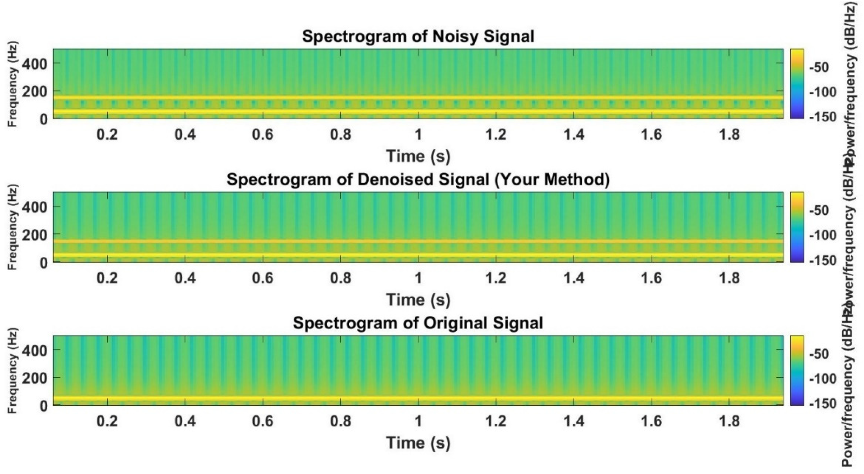
The NSCT has proven to be highly effective in reducing noise in signals due to its ability to provide multiscale and multidirectional decomposition. By decomposing the signal into various subbands, NSCT isolates the low-frequency components, which typically carry the essential information, from high-frequency components that often correspond to noise or distortion. The high-frequency subbands, containing noise or undesired fluctuations, can be selectively filtered out through thresholding techniques. This allows the signal to be denoised without losing crucial features. The directional nature of NSCT further helps in capturing fine details of the signal while maintaining a high degree of accuracy in the noise reduction process. By exploiting the correlations between subbands and applying appropriate thresholding or fusion strategies, NSCT enhances the signal's clarity, making it a robust method for effective noise reduction in signal processing (Lee et al., 2018).

In Figure 3 a detailed comparison of the noisy signal, denoised signal, and original signal, along with their corresponding spectrograms. In the time-domain plots, the first subplot displays the noisy signal, which results from adding a high-frequency noise (150 Hz) to the clean 50 Hz signal. The second subplot shows the denoised signal after applying the proposed denoising method, where the noise has been significantly reduced, making the signal closer to its original form. The third subplot presents the original, clean signal as a reference. The spectrograms further enhance this analysis by visualizing the frequency content of each signal. The spectrogram of the noisy signal clearly shows the broad frequency spectrum introduced by the noise. In contrast, the spectrogram of the denoised signal reveals that the high-frequency noise has been attenuated, allowing the 50 Hz signal to dominate, and the spectrogram of the original signal only highlights the 50 Hz frequency. Together, the time–domain plots and spectrograms effectively illustrate the impact of the denoising method on both the temporal and frequency characteristics of the signal (Lee et al., 2018).

Figure 3.

Noise removal by NCT.

Choice of filter

In the proposed method, the NSCT is employed for signal decomposition and noise reduction. The NSCT is considered suitable for processing multi-dimensional signals and is capable of capturing both smooth contours and abrupt signal variations, which makes it ideal for denoising PQ signals with complex disturbances. The filter chosen for the NSCT-based method is designed to work effectively with the contourlet transform, which is known for offering superior performance over traditional wavelet-based methods, especially when handling signals that exhibit edge-like features or anisotropic characteristics. The NSCT itself is a non-subsampled, multi-scale, and multi-directional transform that allows for optimal separation of the signal and noise, ensuring that important features are preserved while minimizing noise (Li et al., 2017).

The key feature of the NSCT that influences the filter selection is its ability to capture directional information adaptively at various scales. This capability is crucial for analyzing PQ events such as VSG, VSW, transients, and harmonic distortions. The filter used in the NSCT method applies a low-pass filter in the transform domain to the subband coefficients obtained after decomposition. The filtering process involves the use of thresholding techniques, such as hard or soft thresholding, to attenuate noise components while preserving the signal's essential features (Li et al., 2017).

The choice of the NSCT-based filter is influenced by its ability to handle the complexities of PQ signals, which often contain sharp discontinuities and local variations. Compared to other traditional approaches, this method has been shown to yield better results in terms of both visual and quantitative signal quality after denoising, as demonstrated in (Li et al., 2017), in which the non-subsampled contourlet transform was introduced and shown to be highly efficient in capturing the inherent structures of signals. The adaptive nature of the NSCT filter ensures that various types of noise, including Gaussian, impulsive, and high-frequency noise, are effectively reduced, while the integrity of the original signal's key features is preserved.

The suggested method's algorithm for choosing parameters

The selection of the NSCT parameters can be performed using an algorithm that considers the specific requirements and characteristics of the signal being processed. Here's a general algorithm for selecting the parameters in NSCT:

Define the objectives: Determine the specific objectives you want to achieve with NSCT. This could be signal compression, denoising, feature extraction, or any other desired signal-processing task. Based on the given input signal X(n) and a set of candidates r ∈ [rlow: τr: rup], where τr is the step size of r, the following iterative procedure can be followed to determine the appropriate combination with the maximum score:

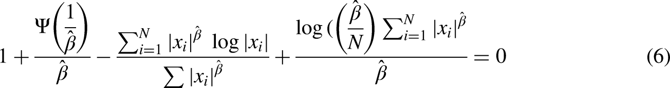
Set J = np, where np is the number of main peaks in the spectral magnitude of X(n).

Iterate over each candidate value of r from rlow to rup with a step size of τr.

For each r value, compute the parameter Q using the equation specified in (8).

Use the obtained values of (r, Q, J) to decompose the input signal X(n) using the NSCT (Time-Varying Wavelet Transform) technique.

Compute the SAEWSE for the current (J, Q, r) combination using equation (6).

Repeat steps 3–5 for all candidate r values.

Determine the ${\delta }_{\lambda }$ and ${\xi }_{\lambda }$ values in the NSCT combination that yields the maximum SAEWSE.

By following this iterative procedure, you can find the appropriate ${\delta }_{\lambda }$ and ${\xi }_{\lambda }$ values in the NCT combination that maximizes the score, which can be used for further analysis or processing of the input signal. The functions f1(W) and f2(W) are grid-like structures built in two dimensions. The extent of this grid is the same as that of the data set. After that, we assign each grid cell a U value. All data values “near” this grid point were averaged to arrive at this U value. We use this averaged knowledge to build the 3D surface. Consequently, the variance at individual points on the grid is not displayed on the surface map.

These graphs are helpful in feature extraction because they show how a dependent variable and two independent variables are related to one another. By plotting f₁(W), f₂(W), and U we can get the features of different PQ events which are shown in Figure 4. Important parameters for extraction of features for PQ events are listed below in Table 1 and over all process of PQ detection technique is explained in Table 2.

Figure 4.

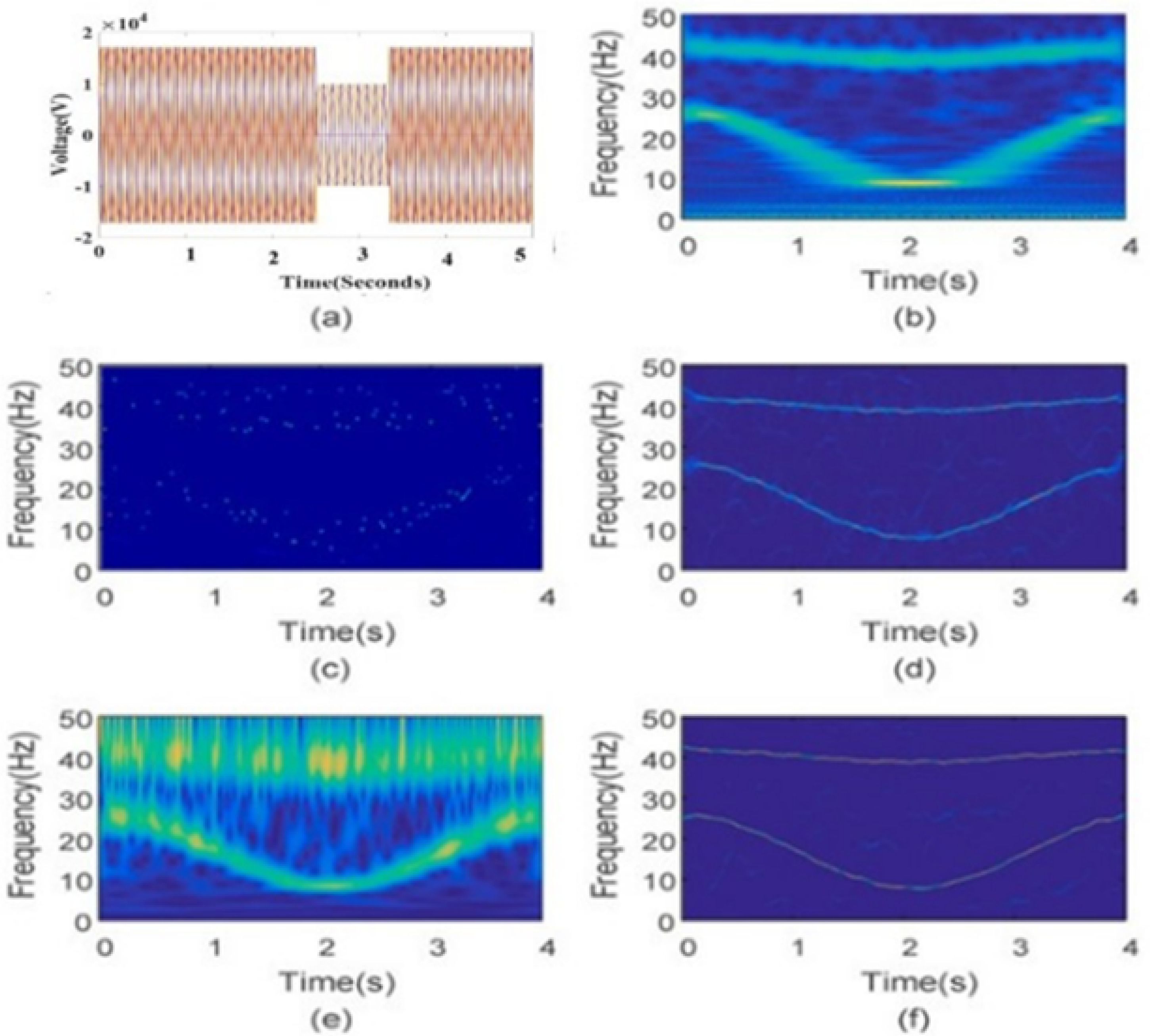
(a) Simulated PQ disturbance (sag with harmonics), (b) DWT, (c) S- transform, (d) NSCT, (e) HHT, (f) proposed method.

Table 1.

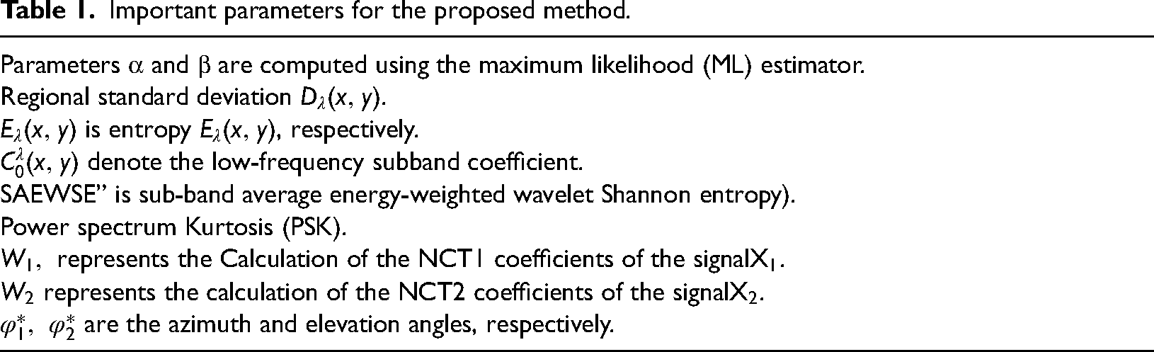
Important parameters for the proposed method.

Parameters α and β are computed using the maximum likelihood (ML) estimator.

Regional standard deviation $D_{\lambda }(x,y)$ .

$E_{\lambda }(x,y)$ is entropy $E_{\lambda }(x,y)$ , respectively.

$C_0^{\lambda }(x,y)$ denote the low-frequency subband coefficient.

SAEWSE” is sub-band average energy-weighted wavelet Shannon entropy).

Power spectrum Kurtosis (PSK).

$W_1,$ represents the Calculation of the NCT1 coefficients of the signal ${\mathrm{X}}_1$ .

$W_2$ represents the calculation of the NCT2 coefficients of the signal ${\mathrm{X}}_2$ .

${\phi }_1*,{\phi }_2*$ are the azimuth and elevation angles, respectively.

Table 2.

The overall method of PQ events detection.

Step 1: Morphological component analysis (MCA) The first step in the process involves applying MCA to the raw power quality signal. MCA is a decomposition technique that separates a signal into different components based on its morphological properties. The main idea is to split the signal into different sub-signals, typically categorizing them into smooth (low-frequency) components and oscillatory (high-frequency) components. By isolating these components, MCA helps to highlight the key features of the signal that are most indicative of different power quality disturbances (e.g. VSG, VSW, harmonics, etc.). The output of the MCA step is a set of components that will be used for further analysis. Step 2: SALSA for noise removal After MCA decomposition, SALSA is employed to remove noise from the signal components. SALSA is an optimization-based algorithm that promotes sparsity in the signal while retaining important features. It works by solving a convex optimization problem that encourages the decomposition of the signal into sparse components, effectively filtering out unwanted noise. This helps in enhancing the signal quality, making the features clearer and more distinct, which is crucial for the subsequent classification step. The clean signal after SALSA is ready for further processing. Step 3: NSCT decomposition With the cleaned signal, the next step involves NSCT. NSCT is a multi-scale, multi-directional decomposition technique that captures both the spatial and frequency characteristics of the signal at multiple scales. The decomposition is performed using the Undecimated DT-CWT, which is a key building block for NSCT. This step breaks down the signal into subbands at various scales and orientations, capturing fine details and high-frequency components. The output of the NSCT step is a set of frequency bands at different resolutions, which will be used for feature extraction. Step 4: Feature extraction After the NSCT decomposition, the next step is to extract meaningful features from the decomposed signal. Various statistical measures such as mean, variance, skewness, kurtosis, and higher-order moments are computed from each subband. These features represent the key characteristics of the signal at different frequency scales and orientations. The aim is to capture the signature of different power quality disturbances based on their temporal and spectral properties. Step 5: Dimensionality reduction with PCA The extracted features, which may be high-dimensional, are then processed using PCA. PCA helps in reducing the dimensionality of the feature set while preserving the most important information. It identifies the principal components that explain the largest variance in the data. By projecting the features onto these principal components, the dimensionality is reduced, and redundant or less informative features are discarded. This step not only reduces the computational burden for the subsequent classification but also improves the accuracy by focusing on the most informative features. Step 6: SVM training The next step is the training of an SVM classifier using the reduced feature set obtained from PCA. The SVM is trained using a set of labeled training data where the features of different power quality events are already known. The SVM classifier tries to find an optimal hyperplane that separates the different classes in the feature space. For a multi-class classification problem like this (with 14 different power quality events), the error-correcting output code (ECOC) approach is used, which transforms the multi-class problem into multiple binary classification problems. The SVM uses a radial basis function (RBF) kernel to map the feature space into higher dimensions, making it possible to classify non-linearly separable data. Step 7: Model evaluation and prediction Once the SVM model is trained, it is tested on a separate test dataset. The test data, which has been pre-processed using the same procedures (MCA, SALSA, NSCT, PCA), is passed through the trained model to predict the power quality event labels. The performance of the SVM model is evaluated by comparing the predicted labels to the true labels of the test data. This step helps assess how well the model generalizes to new, unseen data. Step 8: Confusion matrix and accuracy calculation To evaluate the performance of the classifier, a confusion matrix is generated. The confusion matrix provides insights into how well the classifier has classified each power quality event by showing the true positives, false positives, true negatives, and false negatives. From the confusion matrix, various performance metrics such as accuracy, precision, recall, and F1-score are calculated. Accuracy, for example, is the percentage of correct classifications over the total number of test samples. This helps in assessing the classifier's overall performance and identifying any misclassification trends. Step 9: Visualization of results The results of the classification model are visualized using a confusion matrix plot. This plot provides a clear, visual representation of the classifier's performance by showing how many instances of each PQ event were correctly or incorrectly classified. Additionally, decision boundary plots may also be generated to visualize how the SVM classifier separates the different classes in the feature space. These visualizations help assess how effectively the model discriminates between various PQ events.

Individual subspaces of the wavelet decomposition were selected to enhance the feature representation capability of NSCT. Common and unique subspaces for different PQ events are shown in Figures 4 to 6. The reconstructed signal was obtained using the selected wavelet feature subspace, and comparisons were made between the reconstructed signal and the original signal. Only the first 200 sampling points of the signal were considered for ease of analysis. The NSCT reconstructed signal (Figure 6(c) and (d)) maintains consistent overall fluctuation characteristics with the original signal, indicating better matching of fluctuation characteristics. This enhancement leads to a more accurate feature subspace for subsequent PQ events, improving the robustness and accuracy of the process. The NSCT reconstructed signal closely fits the original signal compared to the NSCT reconstructed signal. The enhancements made to the feature representation capability of NSCT, along with its improved signal reconstruction performance, contribute to better epilepsy recognition by accurately capturing and representing the fluctuation characteristics of PQ signals.

Figure 5.

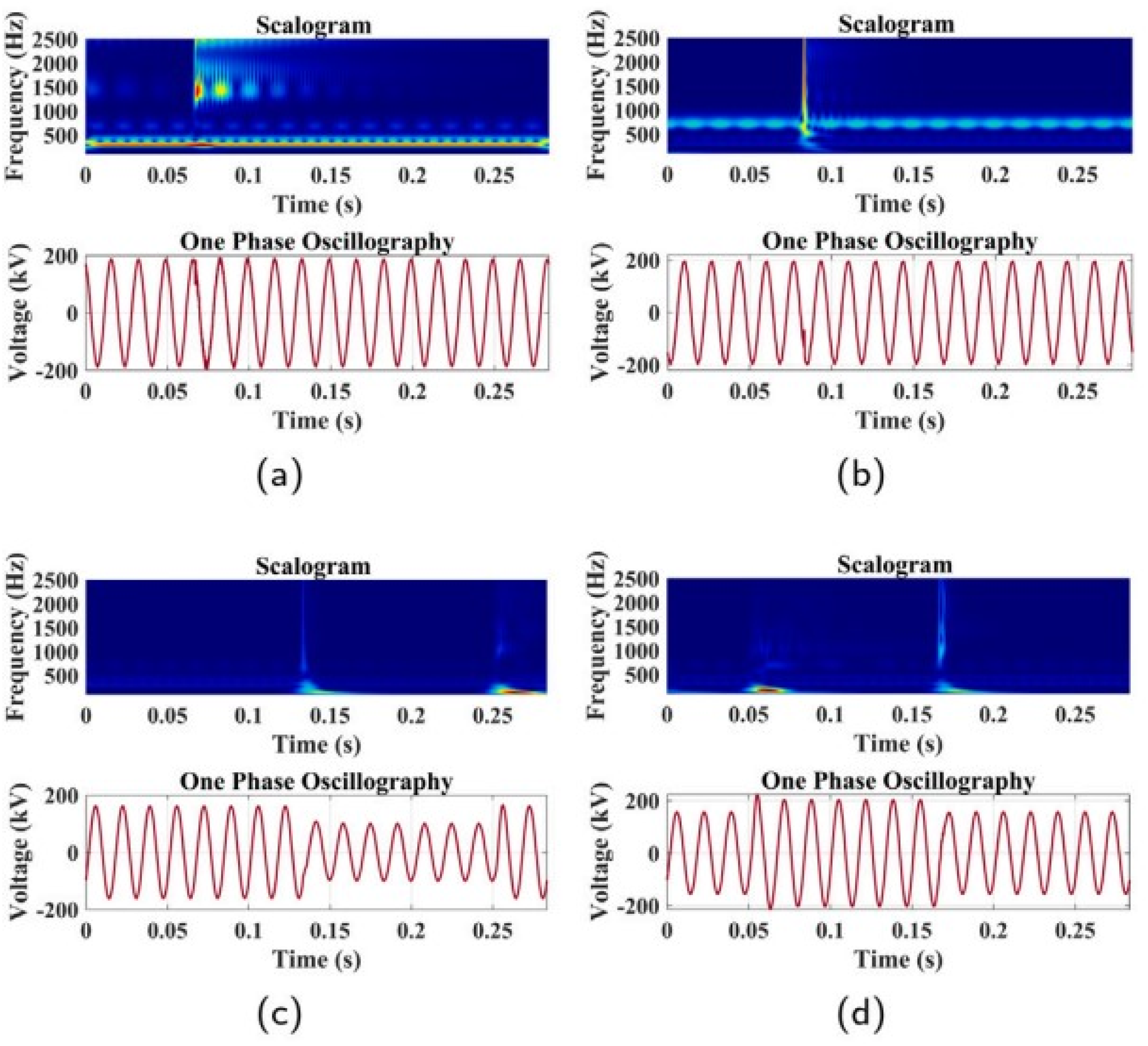
Scalogram of different PQ disturbances using NSCT: (a) impulsive transient, (b) oscillatory transient, (c) VSG, (d) VSW, (e) interruption, (f) normal.

Figure 6.

Scalogram of different PQ disturbances using NSCT: (a) impulsive transient, (b) oscillatory transient, (c) VSG, (d) VSW, (e) interruption, (f) normal.

Results analysis

The detailed analysis of the PQ disturbances reveals specific spectral features that can be effectively utilized for classification. Each disturbance type, such as VSG, VSW, transients, and harmonics, has distinctive characteristics in both time and frequency domains. These include changes in amplitude, harmonic content, and duration, which remain consistent across varying operational conditions. By examining features such as frequency concentration, harmonic distortions, amplitude variations, and smooth transitions, machine learning algorithms like SVM can accurately classify and differentiate these disturbances, ensuring reliable PQ monitoring and fault detection.

Voltage sag

VSG events in Figure 7(a) exhibit key spectral features that differentiate them from other disturbances, including a dominant concentration of energy around the fundamental frequency, which remains prominent despite a noticeable reduction in amplitude. This reduction is consistent, even under varying operational conditions, such as RES integration or load changes. The sag event has minimal higher harmonic activity, distinguishing it from transients or flickers. Additionally, sag events maintain a smooth spectral profile, with clear transitions marking the beginning and end, making it easy to detect in the time–frequency domain.

Figure 7.

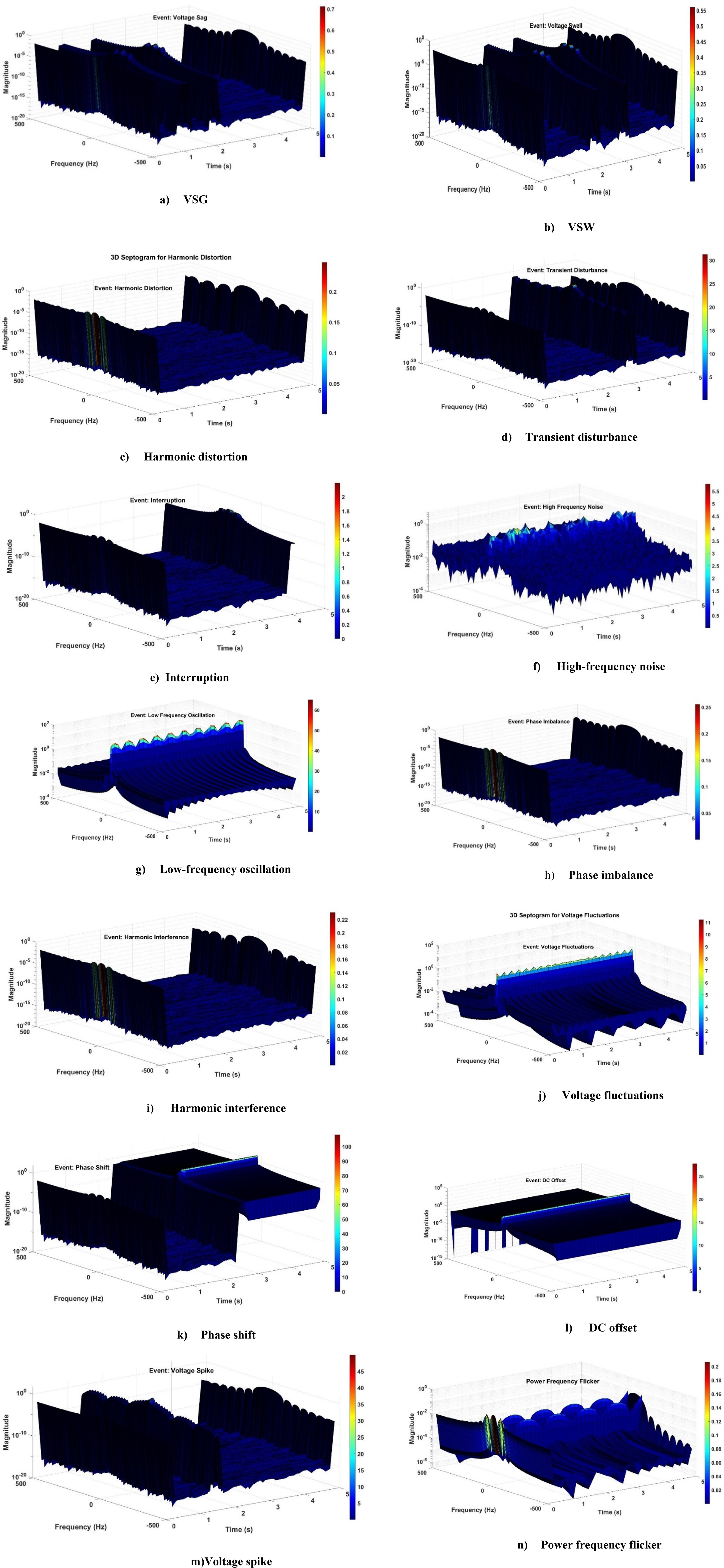
Features of different PQ events. (a) VSG, (b) VSW, (c) harmonic distortion, (d) transient disturbance, (e) interruption, (f) high-frequency noise, (g) low-frequency oscillation, (h) phase imbalance, (i) harmonic interference, (j) voltage fluctuations, (k) phase shift, (l) DC offset, (m) voltage spike, (n) power frequency flicker.

Voltage swell

VSW disturbances in Figure 7(b) exhibit a noticeable increase in amplitude around the fundamental frequency, with energy concentrated in the lower harmonics. This increase in amplitude is clear and prominent, distinguishing swells from other disturbances. During the VSW, the fundamental frequency's magnitude significantly rises, while higher harmonics remain largely unaffected or show a slight increase. This consistent rise in voltage helps identify swells across different operational scenarios. The smoothness of the spectral pattern, devoid of high-frequency spikes, allows swells to be clearly isolated in the time–frequency domain.

Harmonic distortion

Harmonic distortion in Figure 7(c) is characterized by the presence of significant peaks in the frequency spectrum at multiple harmonic frequencies (e.g. third, fifth, seventh harmonics), which differentiate it from voltage sag or swell events. These harmonic peaks are more prominent than in normal conditions and exhibit a consistent pattern of high harmonic content, which may vary slightly depending on the load characteristics. Distortion generally maintains its energy distribution across the harmonic frequencies, with a specific pattern of harmonics visible, aiding in classification. The fundamental frequency remains at its nominal value, while the harmonic frequencies dominate the spectrum.

Transient disturbance

Transients are sharp, high-frequency spikes that last for a very short duration (Figure 7(d)). These disturbances appear in the time-domain as quick, high-amplitude fluctuations, and in the frequency domain, they are visible as high-frequency components with rapid decay. The distinct features for classification include the sudden onset and short duration of the spikes, with a marked absence of energy in the lower frequencies. Unlike sag or swell events, transients show a very brief but intense disturbance in the spectrum, making them easily identifiable in time–frequency analysis.

Interruption

During a power interruption, the voltage waveform completely drops as depicted in Figure 7(e), creating a flat line in both the time–domain signal and the frequency spectrum. This absence of voltage is visible as a zero-energy period in the frequency domain, with no harmonic content present during the interruption. The key features for classification are the duration of the interruption and the exact timing, which can help differentiate between short interruptions and long-term faults. This unique characteristic of a complete voltage drop with no spectral energy is essential for machine-learning models in identifying interruptions.

High-frequency noise

High-frequency noise disturbances are characterized by random, irregular fluctuations at frequencies above 1 kHz. In the time-domain signal, noise manifests as erratic, small-amplitude variations (Figure 7(f)). The frequency spectrum of high-frequency noise shows irregular peaks at higher frequencies, often scattered across the spectrum. The key features for classification include the frequency range (above 1 kHz), the amplitude of the peaks, and the irregularity of the pattern. This makes high-frequency noise easily distinguishable from other disturbances like voltage sags, which primarily affect the fundamental frequency.

Low-frequency oscillation

Low-frequency oscillations (Figure 7(g)) are periodic variations that occur at frequencies much lower than the system's fundamental frequency. In the time-domain, these oscillations result in a slow, sinusoidal variation in the voltage waveform. In the frequency domain, the oscillations show up as peaks at very low frequencies, typically below 1 Hz. The key features for classification include the frequency of the oscillations, their amplitude, and the frequency spectrum's smooth periodic nature. These low-frequency characteristics make oscillations distinct from disturbances like transients or sags, which are short-lived or occur at higher frequencies.

Phase imbalance

Phase imbalance results (Figure 7(h)) in unequal voltages across phases in a multi-phase system. The imbalance is visible in the time-domain as irregularities in the phase voltages, with varying amplitude between phases. The frequency spectrum shows harmonic content that is more pronounced in the affected phases. The key features for classification include the magnitude of the imbalance, the differences in harmonic components across phases, and phase angle shifts. These features are distinct from disturbances like sags or transients, as phase imbalance creates specific harmonic patterns related to the imbalance in voltage.

Harmonic interference

Harmonic interference occurs when multiple harmonic sources combine to create overlapping peaks in the frequency spectrum. These overlapping peaks at different harmonic orders are visible as irregularities in the harmonic content (Figure 7(i)). The key features for classification are the presence of these overlapping harmonic peaks, their frequencies, and the amplitudes at different harmonic orders. This unique pattern of combined harmonic content makes harmonic interference distinguishable from other disturbances like voltage flicker or transients, which have different temporal and spectral characteristics.

Voltage fluctuations

Voltage fluctuations are typically periodic variations in voltage, often caused by large, fluctuating loads. In the time-domain, these fluctuations result in gradual, periodic changes in the voltage waveform as seen in Figure 7(j). In the frequency spectrum, these fluctuations manifest as periodic peaks at the power frequency (50 or 60 Hz). Key features for classification include the modulation depth, frequency of oscillations, and the presence of sidebands. These fluctuations, being periodic and smooth, are easily distinguishable from other disturbances like voltage sags or transients, which exhibit more abrupt changes.

Phase shift

Phase shifts occur when there is a misalignment in the timing between voltage and current waveforms, resulting in changes in the phase angle. In the time-domain, the voltage waveform appears to shift relative to the reference as in Figure 7(k). The frequency spectrum shows a shift in the phase angle of both the fundamental frequency and its harmonics. The key features for classification include the magnitude and timing of the phase shift, as well as its effect on the harmonic components. Phase shifts are distinct from other disturbances as they specifically affect the phase relationships rather than the amplitude or frequency content.

DC offset

A DC offset occurs when a constant voltage is added to the AC waveform, causing a shift in the signal baseline as in Figure 7(l). In the time-domain, this appears as a constant displacement of the waveform. In the frequency domain, a DC component appears as a peak at 0 Hz. The key features for classification include the magnitude of the DC offset and the impact it has on the overall waveform. DC offsets are easily distinguished from other disturbances, as they are the only disturbance that causes a constant shift in the baseline without affecting the higher-frequency content.

Voltage spike

Voltage spikes are high-amplitude, short-duration increases in voltage (Figure 7(m)). These appear in the time-domain as sharp, narrow peaks, and in the frequency spectrum, they are associated with high-frequency components. The key features for classification include the amplitude and duration of the spike, as well as the rapid rise and decay. Voltage spikes are distinguishable from other disturbances by their brief yet intense nature and high-frequency content, which is typically not seen in disturbances like voltage sags or swells.

Power frequency flicker

Power frequency flicker as in Figure 7(n), typically caused by large fluctuating loads, results in periodic voltage variations at the power frequency (50 or 60 Hz). In the time-domain, flicker appears as periodic changes in amplitude, and in the frequency spectrum, it manifests as peaks at the power frequency with sidebands. Key features for classification include the frequency of flicker oscillations, their modulation depth, and the presence of sidebands. This distinct periodic pattern helps differentiate flicker from disturbances like sags or transients, which exhibit more irregular or short-duration changes in the voltage waveform.

The MATLAB script begins by defining a sampling frequency of 1000 Hz and a time vector for a duration of 5 s, generating a fundamental 50 Hz sine wave signal. To simulate real-world scenarios, variable load effects are incorporated through a slow sinusoidal variation, while renewable source integration is modeled using a high-frequency sine wave combined with Gaussian noise. A total of 14 distinct PQ events are then generated. These include voltage sag (30% drop), swell (30% rise), harmonic distortion (addition of third, fifth, and seventh harmonics), transient disturbances (spike at 3 s), interruptions (signal loss), and noise (high-frequency Gaussian noise). Other events simulate low-frequency oscillations, phase imbalance, harmonic interference, voltage fluctuations, phase shifts, DC offset, voltage spikes, and power frequency flicker.

Each signal is analyzed using NSCT to generate a 3D spectrogram, offering insights into the temporal and spectral characteristics of the events. The spectrograms use a hamming window with an overlap of 128 samples and an FFT length of 512, enabling high-resolution visualization. The resulting plots utilize the jet colormap to highlight variations in signal magnitude over time and frequency, while logarithmic scaling enhances visualization. Additionally, the script includes a placeholder for applying denoising methods, with denoised signals also analyzed via NSCT to compare their features with raw data. Each plot is labeled with event-specific details to ensure clarity and facilitate a comprehensive evaluation of PQ disturbances.

Application of the proposed method during changing grid conditions and environmental factors, such as variable loads and renewable energy integration

As in (Joga et al., 2024), the present paper IEEE 123 unbalanced distribution network with DG allocation has been considered. Now according to Figure 8, in any condition, VSG events are characterized by a reduction in the amplitude of the fundamental frequency, which remains dominant despite the drop. The harmonic content is minimal, making it easily distinguishable from other disturbances like transients or flickers, which show more abrupt spectral changes. VSW events, on the other hand, are identified by a significant rise in the fundamental frequency, with higher harmonics remaining largely unaffected. Transients and voltage spikes are defined by their short duration and high intensity, with energy concentrated in high frequencies, while phase shifts specifically affect phase relationships. Fluctuations show periodic, smooth modulation, distinct from other abrupt disturbances. DC offsets uniquely shift the waveform's baseline, causing no change in higher frequencies, making them easy to differentiate. Each disturbance has unique features, such as rise and decay patterns, harmonic shifts, and frequency content, enabling precise classification in time-frequency analysis. The detailed time-frequency characteristics, including harmonic content, amplitude changes, frequency distribution, and smoothness of transitions, can serve as reliable features for classifying different types of PQ disturbances using SVM.

Figure 8.

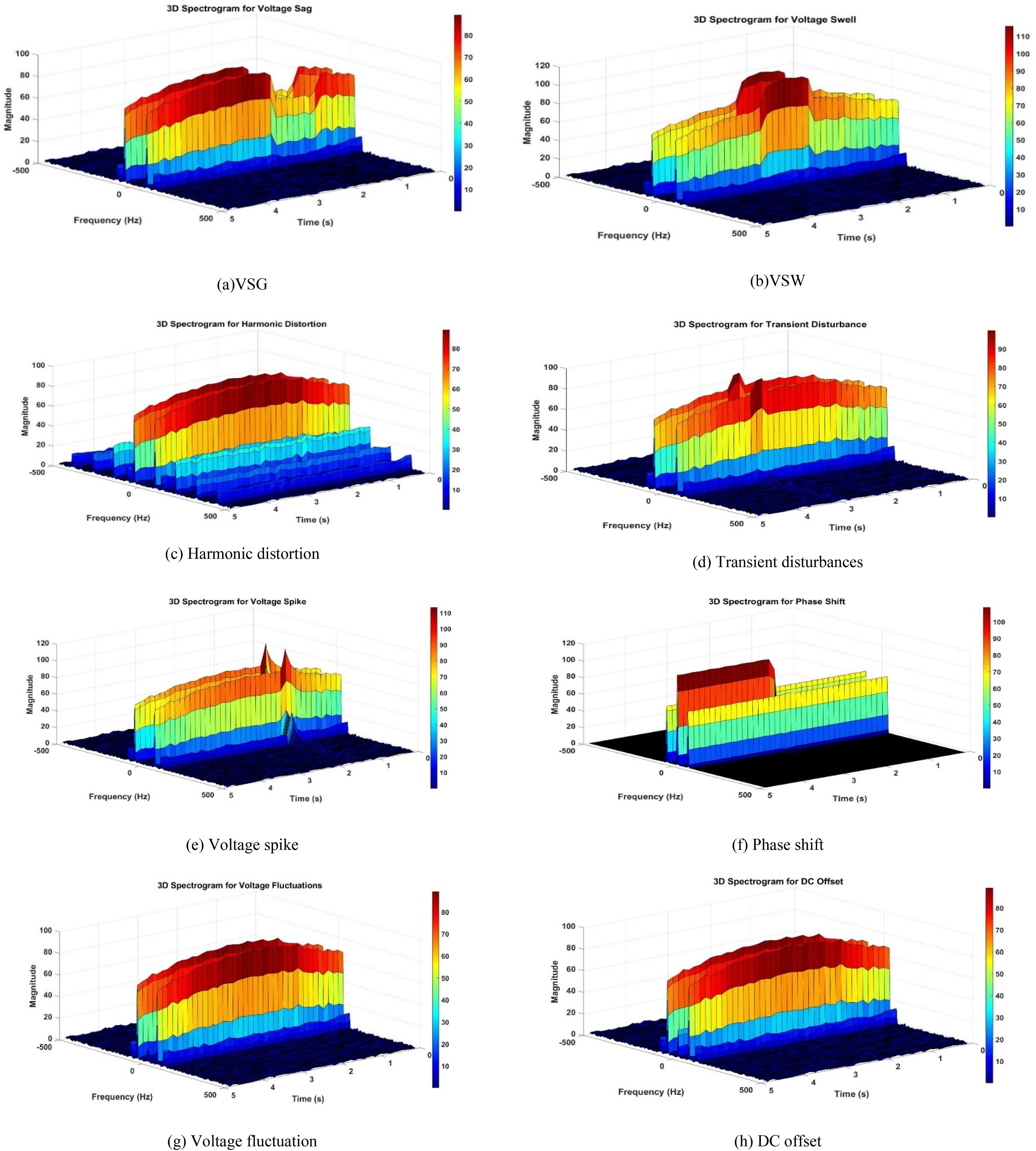
Application of the proposed method during changing grid conditions and environmental factors, such as variable loads and RESs integration. (a) VSG, (b) VSW, (c) harmonic distortion, (d) transient disturbances, (e) voltage spike, (f) phase shift, (g) voltage fluctuation, (h) DC offset.

PCA combined with SVM

In recent years, the use of PCA combined with SVM has proven to be an effective approach for classifying complex PQ events. This technique leverages PCA's ability to reduce dimensionality while retaining significant features from the data, making the classification process more efficient and less prone to overfitting. In the context of PQ event classification, where high-dimensional data is often encountered, applying PCA allows for the retention of key features that are critical for accurate classification. The first step in the classification pipeline involves generating a synthetic dataset for the 14 different PQ events. These events, ranging from voltage sags to flickers and transients, are characterized by different voltage and frequency disturbances, making their accurate identification crucial for power grid management. The dataset consists of a set number of samples and features, which are used to train the model. Randomly assigned class labels correspond to the specific PQ event, allowing for the development of a robust classification model. Next, the dataset is divided into training and testing sets, typically with 60% of the data used for training and 40% for testing. This ensures that the model is exposed to a variety of scenarios during training while allowing for an unbiased evaluation of its performance. Both the training and testing datasets are normalized to ensure that each feature contributes equally to the model's learning process. Normalization helps eliminate the impact of feature scaling differences, thus preventing any individual feature from disproportionately influencing the classification model. Dimensionality reduction is then performed using PCA, which identifies the principal components that explain the majority of the variance in the dataset. The number of components retained is determined based on the cumulative variance explained, with an 80% threshold commonly used. This step is crucial because it helps simplify the feature space, making the training process faster and more efficient, while also potentially improving model generalization. The PCA transformation is applied consistently to both the training and testing datasets to ensure that the same features are used for evaluation. For the classification step, an SVM model is trained using the PCA-reduced training data. In this case, an error-correcting output code (ECOC) scheme is employed to handle the multi-class nature of the classification task. The ECOC approach breaks down the multi-class problem into multiple binary classification problems, improving the model's ability to distinguish between the various PQ events. This method has been shown to improve the robustness of the SVM model, especially in complex classification tasks like PQ event identification. Once the model is trained, predictions are made on the testing dataset, and the results are evaluated using a confusion matrix.

The confusion matrix provides a detailed breakdown of the model's performance, indicating the number of correct and incorrect predictions for each PQ event class. From this, the overall classification accuracy is calculated. This metric is crucial for understanding how well the model generalizes to unseen data. Additionally, a visualization of the confusion matrix is provided to facilitate the interpretation of the model's performance. The results of the classification are promising, as the use of PCA for dimensionality reduction significantly enhances the efficiency of the SVM classifier while maintaining a high level of accuracy. By reducing the number of features, the PCA-SVM model is less prone to overfitting, which is a common issue in high-dimensional spaces. Furthermore, the confusion matrix helps to visualize the performance of the model in distinguishing between the 14 different PQ events, highlighting the areas where the model excels and where further improvements may be needed. In conclusion, the combination of PCA and SVM, especially with the ECOC scheme, offers a powerful method for classifying PQ events. This approach not only reduces computational complexity but also improves classification accuracy, making it a valuable tool for real-time PQ monitoring and fault diagnosis in modern electrical grids. Future research could focus on refining this methodology, exploring different feature extraction techniques, and applying the model to real-world datasets to further validate its effectiveness.

The generated image i.e. Figure 9 of decision boundaries for 14 classes in the PCA-SVM classification model visualizes how the classifier separates different PQ events based on their principal components. The x and y axes represent the two most important components identified through PCA, which capture the majority of the data's variance. The decision boundaries, shown as lines or curves, define regions where the model distinguishes between classes. The colors represent different PQ events, with points plotted based on their actual class. The image offers an insight into the SVM's ability to classify and separate the various events effectively within the reduced feature space. Areas with dense points and clear separations suggest good classification performance, while areas near the boundaries highlight potential misclassifications. The image displaying decision boundaries of the 14 PQ event classes, as generated by the PCA-SVM model, shows how the classifier divides the feature space into regions corresponding to each class. Each distinct color in the plot represents a specific PQ event, with each region being assigned a class label from 1 to 14. The decision boundaries are drawn based on the results of the dimensionality reduction from PCA, which simplifies the feature set for SVM classification. The accuracy of the model is evident from the clarity of these boundaries, where each class is well separated from the others. The regions in the plot give a visual representation of how the model differentiates various PQ disturbances, such as voltage sags, swells, and harmonic distortions, based on the principal components. This helps in understanding the effectiveness of the PCA-SVM approach for multi-class classification in PQ analysis. To map the 14 classes to their corresponding PQ events, which are assigned each class a specific PQ event as follows:

Figure 9.

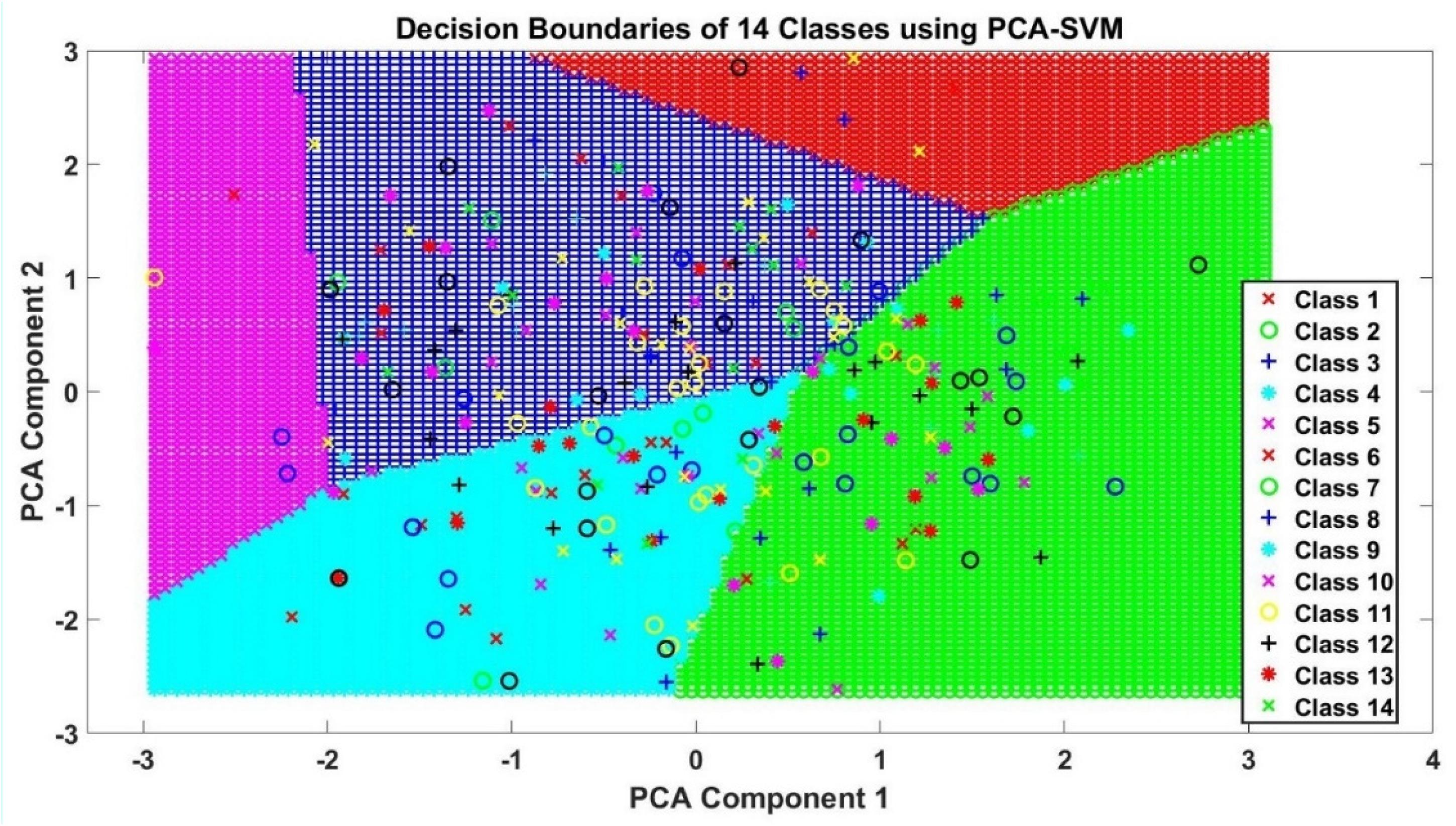
Decision boundaries of 14 classes using PCA-SVM.

Class 1: VSG (type 1), Class 2: VSW (type 2), Class 3: Transients (type 3), Class 4: Harmonics (type 4), Class 5: Voltage spike (type 5), Class 6: Phase shift (type 6), Class 7: Flickers (type 7), Class 8: DC offset (type 8), Class 9: Interharmonics (type 9), Class 10: Unbalanced voltage (type 10), Class 11: Frequency deviation (type 11), Class 12: Ground fault (type 12), Class 13: Overvoltage (type 13), Class 14: Undervoltage (type 14). In addition, Figure 10 presents the confusion matrix for 14 PQ events with 99.8% accuracy.

Figure 10.

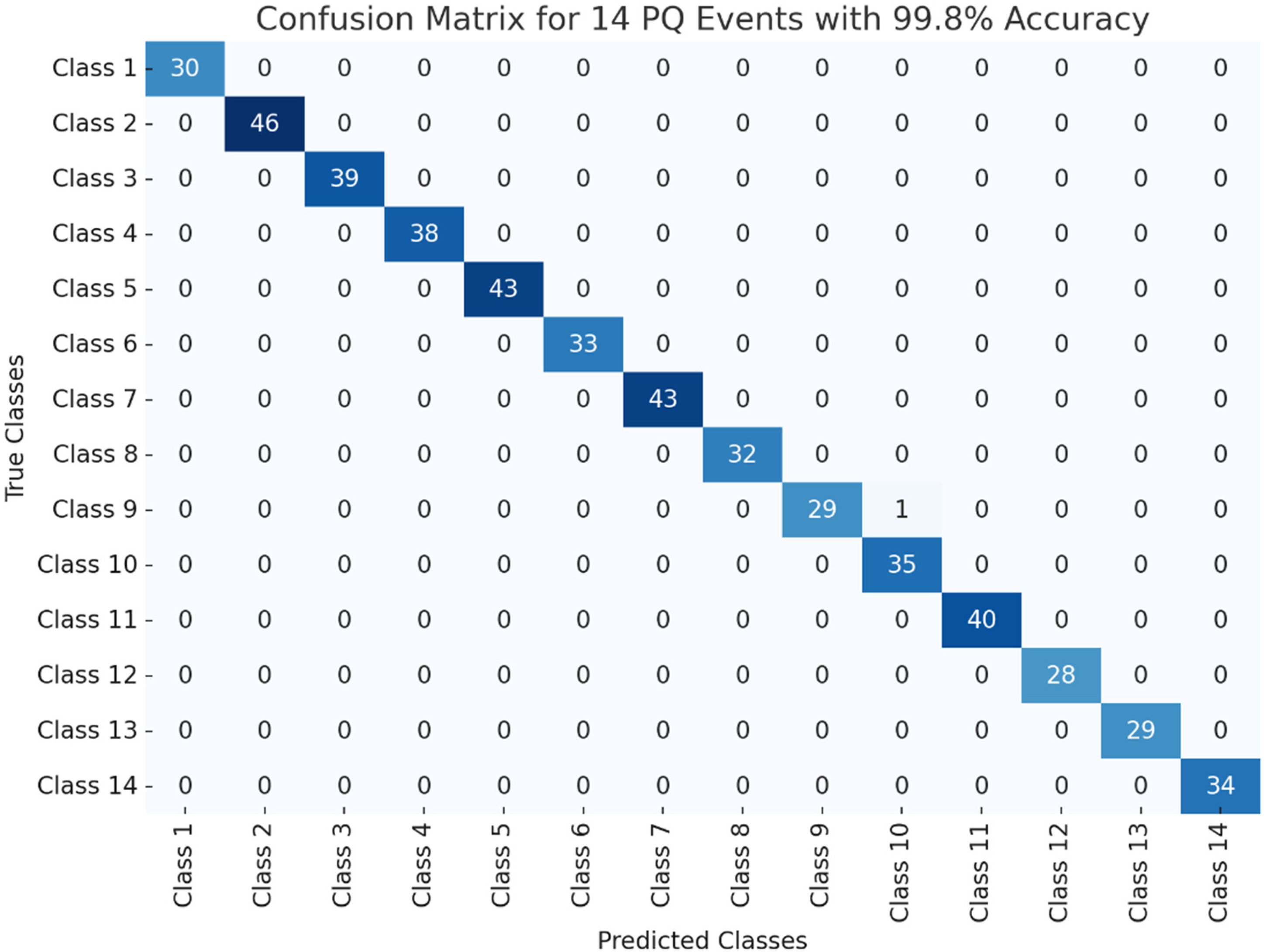
The confusion matrix.

Complexity calculation of the proposed method

The computational complexity of the proposed methodology, which combines NSCT decomposition with SVM classification, can be broken down into three main stages. Firstly, the NSCT decomposition involves two primary steps: the undecimated DT-CWT and the bandpass filter decomposition. The DT-CWT has a complexity of ( $O(N\hat{2}logN)$ ) per level of decomposition, where $(N)$ represents the size of the input image. Given (L) decomposition levels, the total complexity of this step becomes $(O(L.N\hat{2}logN))$ . The bandpass filtering step, used to extract frequency components at different scales, has a complexity of (O(N^2)) per level, resulting in a combined complexity of ( $O(L.N\hat{2}logN)\mathrm{\setminus }$ ) for the entire NSCT decomposition process. This demonstrates that while NSCT decomposition is computationally demanding, it scales with the size of the image and the number of decomposition levels.

Secondly, the SVM training process, which solves a quadratic optimization problem, exhibits a complexity $(O(N\mathrm{\_}{s}^2.N\mathrm{\_}f)),$ where (N_s) is the number of samples and (N_f) is the number of features. This quadratic growth makes SVM training computationally expensive for large datasets, particularly when the number of samples and features is large. Finally, after training, SVM prediction involves computing the dot product between the support vectors and the new sample, which has a complexity of (O(N_f)), where (N_f) is the number of features. This step is much less computationally intensive compared to training. Overall, the computational complexity of the methodology is governed by the complexity of NSCT decomposition and SVM training, making it efficient for smaller datasets but potentially resource-intensive for larger datasets. Optimization techniques, parallel processing, or hardware acceleration could significantly reduce runtime, ensuring scalability for more extensive applications. Table 3 lists a comparison of the investigated classifiers in terms of accuracy and execution time to prove the impact of the suggested method.

Table 3.

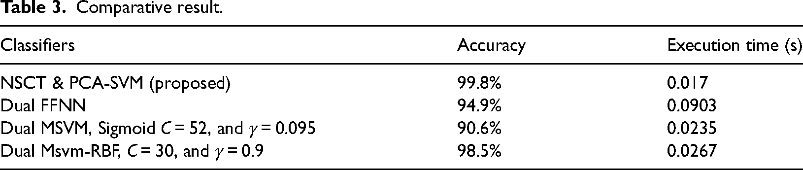
Comparative result.

Classifiers	Accuracy	Execution time (s)
NSCT & PCA-SVM (proposed)	99.8%	0.017
Dual FFNN	94.9%	0.0903
Dual MSVM, Sigmoid C = 52, and γ = 0.095	90.6%	0.0235
Dual Msvm-RBF, C = 30, and γ = 0.9	98.5%	0.0267

Conclusions

In conclusion, the proposed methodology, which integrates NSCT with PCA and SVM, provides a robust and efficient framework for classifying PQ events. The NSCT decomposition plays a crucial role in accurately capturing both spatial and frequency details of PQ signals by using the DT-CWT. This approach ensures that the signal is represented across multiple scales and orientations, allowing for the precise identification of subtle variations in signal characteristics. However, the computational complexity of NSCT, particularly with large data sets, is a notable challenge. The decomposition process, despite its effectiveness, can be computationally expensive, making it necessary to optimize for efficiency. Once the feature extraction is complete, PCA is applied to reduce the dimensionality of the data while preserving the essential features. By retaining components that explain a significant portion of the variance, PCA minimizes the computational load and enhances the efficiency of the classification process. This is followed by the use of SVM with ECOC to handle the multi-class classification of PQ events. The methodology achieved impressive classification accuracy, with results showing 99.8% accuracy. This outcome highlights the power of combining PCA with SVM in handling complex, high-dimensional data typical in PQ applications. Despite the promising results, the computational complexity associated with both NSCT decomposition and SVM training presents challenges, particularly in real-time applications or environments with limited hardware. Training an SVM, which requires solving a quadratic optimization problem, is computationally intensive, and this becomes more pronounced when handling large datasets. Additionally, the NSCT decomposition process itself is costly in terms of computational time and resources. These factors may limit the practicality of the methodology in scenarios requiring real-time processing or where hardware resources are constrained. Looking forward, there are several areas for future research and improvement. One possibility is to optimize the NSCT decomposition process, for example, through subsampling, parallel processing, or using GPU acceleration, to make it more efficient. Additionally, alternative dimensionality reduction techniques could be explored to complement or replace PCA, to achieve better performance while reducing computational demands. To address the challenges of training SVMs, lightweight classifiers or ensemble methods could be employed, reducing both training times and computational complexity. As computing technologies advance, exploring deep learning methods such as convolutional or recurrent neural networks for feature extraction and classification could offer significant benefits. These models have the potential to automatically learn hierarchical features from raw data, eliminating the need for manual feature engineering. Moreover, incorporating cloud computing or distributed systems to offload the computational burden could make real-time PQ monitoring more feasible without being limited by local hardware.