
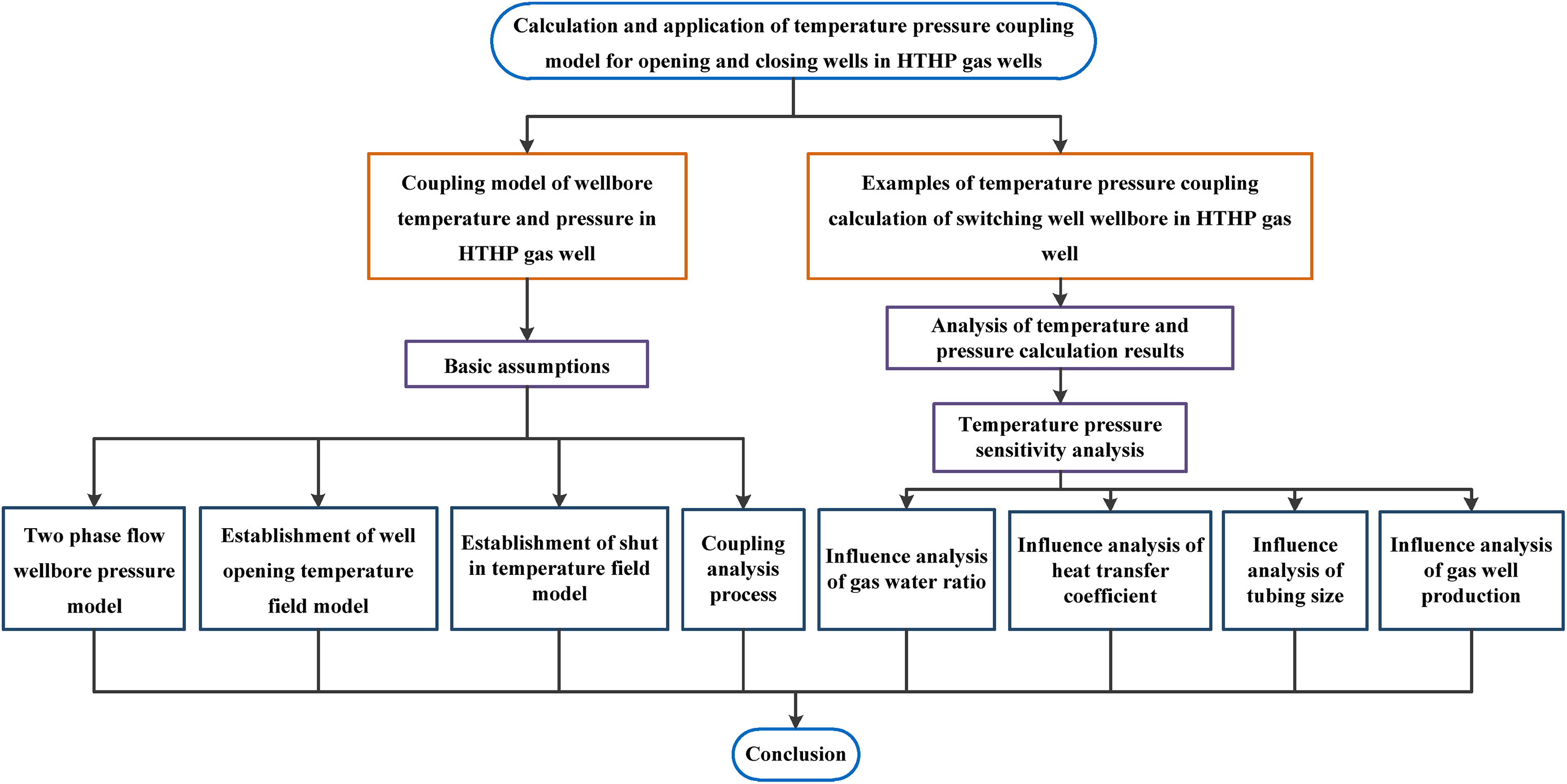
Abstract
Switching wells in high-temperature and high-pressure gas wells will affect parameters such as the temperature and pressure of the fluid in the wellbore. Dynamic monitoring of temperature and pressure is difficult, and wellbore temperature, pressure, and fluid physical parameters are coupled to each other. Obtaining them separately will lead to large calculation errors. In order to improve the prediction accuracy of temperature and pressure in high-temperature and high-pressure gas wells, Based on the temperature–pressure coupling algorithm, this study compares the advantages and disadvantages of nine classic algorithms based on the temperature–pressure coupling algorithm, considers the impact of high temperature and high pressure on the temperature and pressure of the gas wellbore fluid, and establishes an unsteady temperature–pressure coupling model for high-temperature and high-pressure gas wells under on–off well conditions. Comparing with the measured data, it is proved that the prediction accuracy of the unsteady temperature–pressure coupling model of high-temperature and high-pressure gas wells meets the construction requirements of switch wells. The established model is used to simulate the temperature and pressure distribution of two high-temperature and high-pressure gas wells under switching conditions. The analysis shows that the distribution of wellbore temperature and pressure under the switch on and off conditions is affected by the gas–water ratio, heat transfer coefficient, tube size, and gas well production. Among them, the gas–water ratio increased by 1.5 times, the wellhead temperature increased by 25%, and the wellhead pressure decreased is 7.68%; When the heat transfer coefficient is increased by 1.5 times, the wellhead temperature drops to 34.38% and the wellhead pressure drops to 2.29%. When the tube size is increased by 1.125 times, the wellhead temperature is reduced by 44.20% and the pressure is increased by 6.09%. When the production of gas well is doubled, the wellhead temperature increases by 40.79% and the wellhead pressure decreases by 2.29%. The results can be used as a basis for the construction of high-temperature and high-pressure gas wells.
Introduction
With the continuous increase in energy demand, the focus of oil and gas exploration has gradually shifted to high-temperature and high-pressure wells with complex formations. Compared with normal temperature and normal pressure wells, the distribution of wellbore temperature and pressure at different times when high-temperature and high-pressure gas wells are on and off is more complex and dynamic monitoring is also more difficult (Huan et al., 2021; Wang et al., 2020). Many existing conventional monitoring process methods and interpretation techniques often cannot meet monitoring needs (Wang et al., 2019; Galvao et al., 2019), and theoretical analysis must be used to predict the distribution of wellbore temperature and pressure. In addition, in actual production, it was also found that the wellbore temperature will change after the shut-in of a high-temperature and high-pressure gas well, resulting in changes in fluid physical parameters and liquid phase settlement. The wellbore pressure distribution will also change, and the pressure profiles at different depths will change greatly. Therefore, it is of great practical significance to improve the prediction accuracy of wellbore temperature and pressure distribution during the opening and closing of high-temperature and high-pressure gas wells and guide their efficient development.
Since the 1930s, scholars at home and abroad have begun to explore and study the prediction of wellbore temperature field (Rui et al., 2020). The earliest written data on the downhole temperature distribution was in 1937. Schlumberger et al. (1937) and others proposed a method to predict the fluid temperature in the wellbore. In 1962, Ramey (1962) proposed the wellbore temperature prediction method when injecting fluid. In order to simplify the model, the dimensionless time function and total heat transfer coefficient are introduced, and the correctness of the model is verified by an example. Its model has been recognized as the basis of the wellbore temperature prediction model. Then, Willhite (1967) improved the Ramey model, combined the total heat transfer coefficient and the heat transfer characteristics between the wellbore and the formation to calculate the transverse heat loss, proposed the approximate calculation formula of the total heat transfer coefficient in the Ramey model, and estimated the radiation heat transfer coefficient and the convection heat transfer coefficient. Subsequently, Shiu and Beggs (1980) and Hagoort (2004) simplified the solution process of the Ramey model and made the Ramey model more perfect for the problem that the calculation accuracy of the Ramey model was not high at the initial stage of production. After basically meeting the requirements of the calculation model of the steady-state temperature field, the scholars have noticed the importance of the temperature and pressure changes during the switching on and off period. In 2009, Haiquan et al. (2009) combined the mass conservation equation and the momentum conservation equation to establish a temperature prediction model for stable production gas wells and a wellbore temperature model under shut-in conditions, and analyzed the changes in wellhead and bottom hole pressure during the shut-in process. However, they only calculated the temperature field without parameter coupling, and the results are quite different from the actual ones. In 2010, Zhenghe et al. (2010) in order to obtain the bottom hole pressure in the shut-in test more accurately, based on Hasan et al. (2005) research, considered the fluid phase change and proposed the wellbore unsteady heat transfer model corresponding to the shut-in state of high-temperature and high-pressure gas wells, which can effectively reflect the change of wellbore temperature and pressure after shut-in. Abdelhafiz et al. (2021) and Zhang et al. (2019) pay special attention to the calculation of gas wells in the sea. Up to now, the prediction model of wellbore temperature and pressure has developed from one-dimensional to multidimensional, and from steady state to unsteady state (Zheng et al., 2020).
With the continuous deepening of scholars and the continuous optimization of various parameters of the model, the calculative accuracy of the model is also improving, but the performance of the wellbore in the shut-in process has been less studied. Therefore, this study provides a theoretical basis for the analysis of the production performance of high-temperature and high-pressure gas wells by establishing a model of the nonstationary temperature and pressure coupling. The focus of this study is to establish a coupling model of temperature and pressure for the opening and closing of the wellbore of a high-temperature and high-pressure gas well. From the point of view of heat transfer, based on the law of heat transfer between the wellbore and the formation, considering the Joule-Thomson effect, and combining the energy conservation equations, the wellbore unsteady temperature prediction model corresponding to the opening and closing of the well is established.
Coupling model of wellbore temperature and pressure in HTHP gas wells
Basic assumptions
As shown in Figure 1, the well-structure diagram of high temperature and high pressure is shown. Before establishing the prediction model of wellbore temperature and pressure, it is necessary to make some simplifications. The assumptions are as follows:
The temperature, pressure, and gas parameters of each point on any section in the wellbore are equal. The temperature of the stratum along the vertical direction is linear, that is, the geothermal gradient is constant. The heat loss of the wellbore and surrounding environment is radial transfer, and there is no heat loss along the well depth direction. Friction heat generated during fluid flow is ignored. Concentric oil casing. Normal production before shut-in. In the calculation, it is assumed that the wellbore temperature corresponding to the production is continuous with the wellbore temperature after the shut-in. After shut-in, the fluid in the well stops flowing immediately, in a static state. The steady-state multiphase pipe flow model is used to calculate the initial pressure of the wellbore, and the prediction of temperature is calculated according to the stable heat transfer of the wellbore and the unstable heat transfer of the formation.
High-temperature and high-pressure wellbore structure diagram.
Two phase flow wellbore pressure model
After a period of production, the water production of the gas well will gradually increase, turning the pure gas well into a gas well; therefore, considering the existence of two phases in the wellbore. For gas wells with a high gas–water ratio, the liquid phase is less abundant, so it can be approximately regarded as a single-phase pipe flow to calculate the pressure; with the continuous increase of water production, a two-phase flow pattern will be generated in the pipe string. At this time, it can no longer be approximated as a single-phase flow and a gas–liquid two-phase pipe flow model needs to be used.
Combined with the relevant data in the Railroad gas field and Govier gas field (Govier and Fogarasi, 1975; Rendeiro and Kelso, 1988), the calculated results of nine pressure drop models are compared with the measured bottom hole pressure. The comparison analysis is shown in Figures 2 and 3.
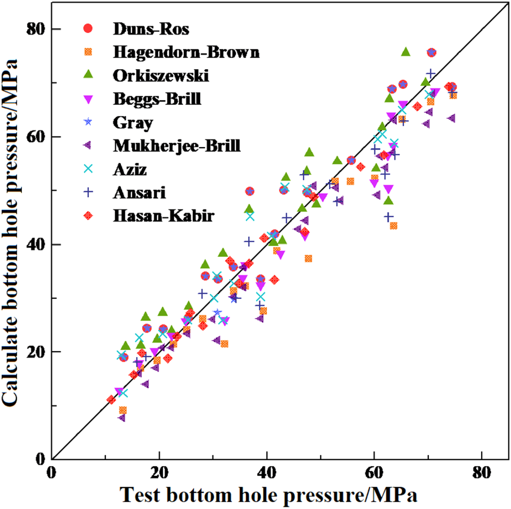
Comparison between measured values of Railroad gas field and calculated values of different pressure drop models.
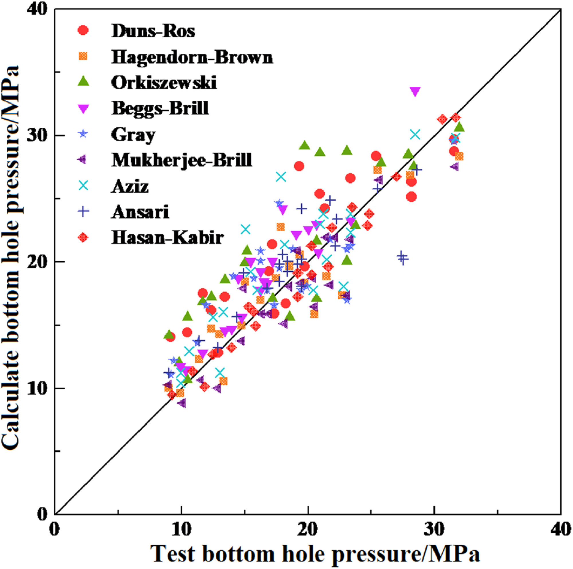
Comparison between measured value of Govier gas field and calculated value of different pressure drop models.
As can be seen from Figures 2 and 3, the results obtained by Duns-Ros, Orkiszewski, and Aziz models are slightly larger than the measured values among the nine calculation models for the pressure drop; the results for the Mukherjee Brill model are smaller than the measured values; the results of the Hagedorn-Brown, Beggs-Brill, Gray, and Ansari models are relatively accurate and close to the measured data for the gas field.
The average relative error represents the overall deviation of the model, and the percentage standard deviation represents the dispersion of the model's calculation results. Two parameters are used to evaluate the accuracy of the various calculation models, calculated as follows:
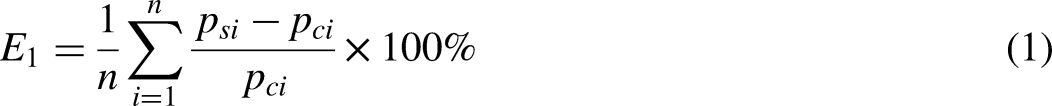
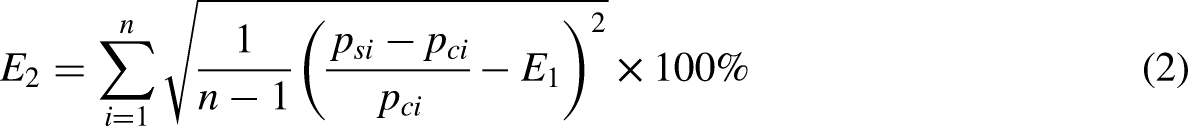
where, E1—Average relative error;
E2—Percent standard deviation;
psi—Calculated bottom hole pressure, MPa;
pci—Measured bottom hole pressure, MPa.
The error values obtained by each model corresponding to different evaluation indexes are sorted and compared, as shown in Figure 4 (Duns and Ros, 1963; Hagedorn and Brown, 1965; Orkiszewski, 1967; Beggs and Brill, 1973; Gray et al., 1978; Mukherjee and Brill, 1985; Aziz and Govier, 1972; Ansari et al., 1990; Hasan et al., 2010).
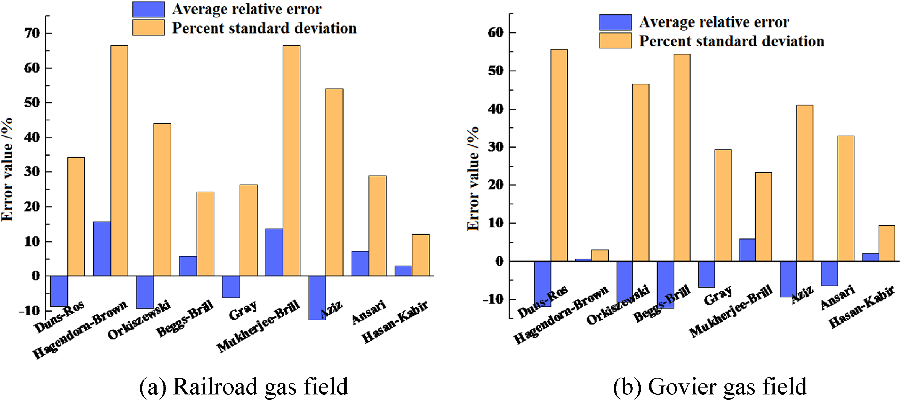
Error of bottom hole pressure calculated by each model.
In a comprehensive comparison of the accuracy and applicability of the various calculation models, the Hagendorn-Brown model, Gray model, and Hasan-Kabir models are found to have higher calculative accuracy among the wellbore pressure models. However, since the Gray model is originally a calculation model for condensate gas wells, and a large part of the test data is from condensate gas wells, the applicability of the Gray model to other types of gas wells cannot be inferred. The Hagendorn-Brown model is an empirical model based on actual data, and its accuracy is also verified by example; the Hasan-Kabir model and Ansari model are theoretical models, and the Hasan-Kabir model has a higher calculative accuracy and a wider application range than the Ansari model. Therefore, based on various factors, the Hasan-Kabir model has been chosen to calculate the pressure drop of two-phase pipe flow in the HTHP gas wells.
Establishment of well opening temperature field model
According to the energy conservation theorem, the total energy in the isolated system remains constant. Microscopic elements are regarded as a closed system. The energy of the fluid entering the microelement is equal to the sum of the energy of the fluid leaving the microelement and the energy loss. In any control volume unit of the wellbore, the energy conservation equation can be expressed as:


where,
g—Gravitational acceleration, 9.8 m/s2;
z—Shaft length, m;
ν—The average velocity of the fluid in the horizontal plane, m/s;
q—Fluid radial heat flow, J/(m·s).
Ordinary differential equation of gas temperature:

where,

where, rto—Inner diameter of oil pipe, m;
Uto—Total heat transfer coefficient, W/(m2·°C);
Th—Second interface temperature, °C;
CJ—Joule Thomson coefficient, °C/MPa;
Cp—Specific heat at constant pressure of fluid, J/(kg·°C);
ke—Formation heat transfer coefficient, W/(m·°C);
Te—Formation temperature, °C; Te = Tebh−gTz;
f (t)—Formation, transient heat transfer function, dimensionless;
w—Gas mass flow, kg/s.
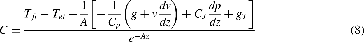
The wellbore is divided into multiple units. When calculating the temperature, it is considered that the fluid physical parameters are constant in each unit, that is, Cp, gT, dv/dz, and dp/dz remain unchanged, and the general solution of formula (3) is obtained:

where, C—Undetermined coefficient;
gT—Geothermal gradient,°C/m.
The definite solution conditions of the first-order linear ordinary differential equation for fluid temperature and depth are z = zin, Tf = Tfi, and Te = Tei. Substitute the above formula to get:
Substitute the value of C into equation (5) to obtain:

where, Tfo—Wellbore fluid temperature at outlet, °C;
Teo—Formation temperature at outlet, °C;
Δz—Vertical length of unit body, m;
Cm—Isobaric heat capacity of gas, J/(kg·°C);
Tfi—Wellbore fluid temperature at inlet, °C;
Tei—Formation temperature at inlet, °C.
Establishment of shut-in temperature field model
During the shut-in, the wellbore is a single-phase fluid, that is, a gas, and the fluid in the wellbore and the formation will no longer flow and will remain a static state. At this point, the frictional heat generation and convective heat transfer caused by fluid flow disappear, and the kinetic energy term need not be considered; coupled with the reason that the gas no longer flows, there is no mass flow. After shut-in, there is still heat transfer between the wellbore and the formation. If the shut-in time is indefinite, the temperature in the well will be close to the formation temperature. Combined with the energy conservation theorem, the change in energy is equivalent to the change in internal energy and the heat absorbed by the cement sheath and the oil casing. The energy conservation equation can be expressed as:

where, Q—Heat flow, J/s;
E—Fluid internal energy, J/kg;
m—Fluid mass, kg;
E'—Internal energy of wellbore system, J/kg;
m'—Wellbore system quality, kg;
t—Shut-in time, s.
Ordinary differential equation of gas temperature:

where, CT—Wellbore heat storage coefficient, dimensionless. Generally, it can be taken as 2.0 after shut-in;
L'R—Hasan relaxation distance (Hasan and Kabir, 1991), m;
Tei—Formation temperature at inlet, °C.
Solve equation (11):

where,

Substitute initial condition Tf=Tf0. When Δt = 0, the fluid temperature corresponding to the shut-in time can be calculated, and the expression is:

Where, Tf0—wellbore fluid temperature at shut-in time, °C;
Tei—Formation temperature, °C;
t—Shut-in time, s.
Equation (14) is the energy conservation equation describing the transient flow during gas shut-in. Assuming that the wellhead temperature can be obtained in real-time, the temperature distribution along the wellhead to the bottom of the well can be calculated from the above formula.
Coupling analysis process
When calculating the wellbore temperature and pressure, the iterative calculation is carried out by assuming the initial value, substituting it into the model, comparing the results, and judging the accuracy. The flow of coupling calculation is shown in Figure 5. The specific method is as follows:
Select the spacing Δz along the well depth direction to divide the pipe string into n sections, and each section is a unit control body; Assuming the initial value of wellbore temperature and pressure, its initial temperature Ti is equal to the original formation temperature, and the wellbore initial pressure Pi is equal to the static gas column pressure; Taking the initial temperature and pressure as the inlet temperature and pressure of the first unit control body, and using the initial temperature and pressure to calculate the fluid physical parameters at the initial time; Select the applicable pressure model according to different phase states and flow patterns of the fluid, and calculate the temperature To and pressure Po at the outlet of the unit control body according to the temperature model and pressure model; Take the average value of temperature and pressure at the inlet and outlet of the unit control body, and calculate the new fluid physical parameters based on the calculation results; Calculate the temperature To’ and pressure Po’ at the outlet again by using the fluid physical parameters calculated in (5); Compare the calculation results obtained in (4) and (6) to judge whether they meet the calculation accuracy requirements. If the requirements are not met, return To’ and Po’ as initial values to step (3) for recalculation until the accuracy requirements are met. After the calculation results meet the requirements, take To’ and Po’ as the initial values at the entrance of the next unit to continue the calculation and repeat (3) ∼ (7) until the bottom of the well; After completing the calculation of the whole well section, the temperature, pressure, and physical parameters at each depth of the wellbore can be obtained.
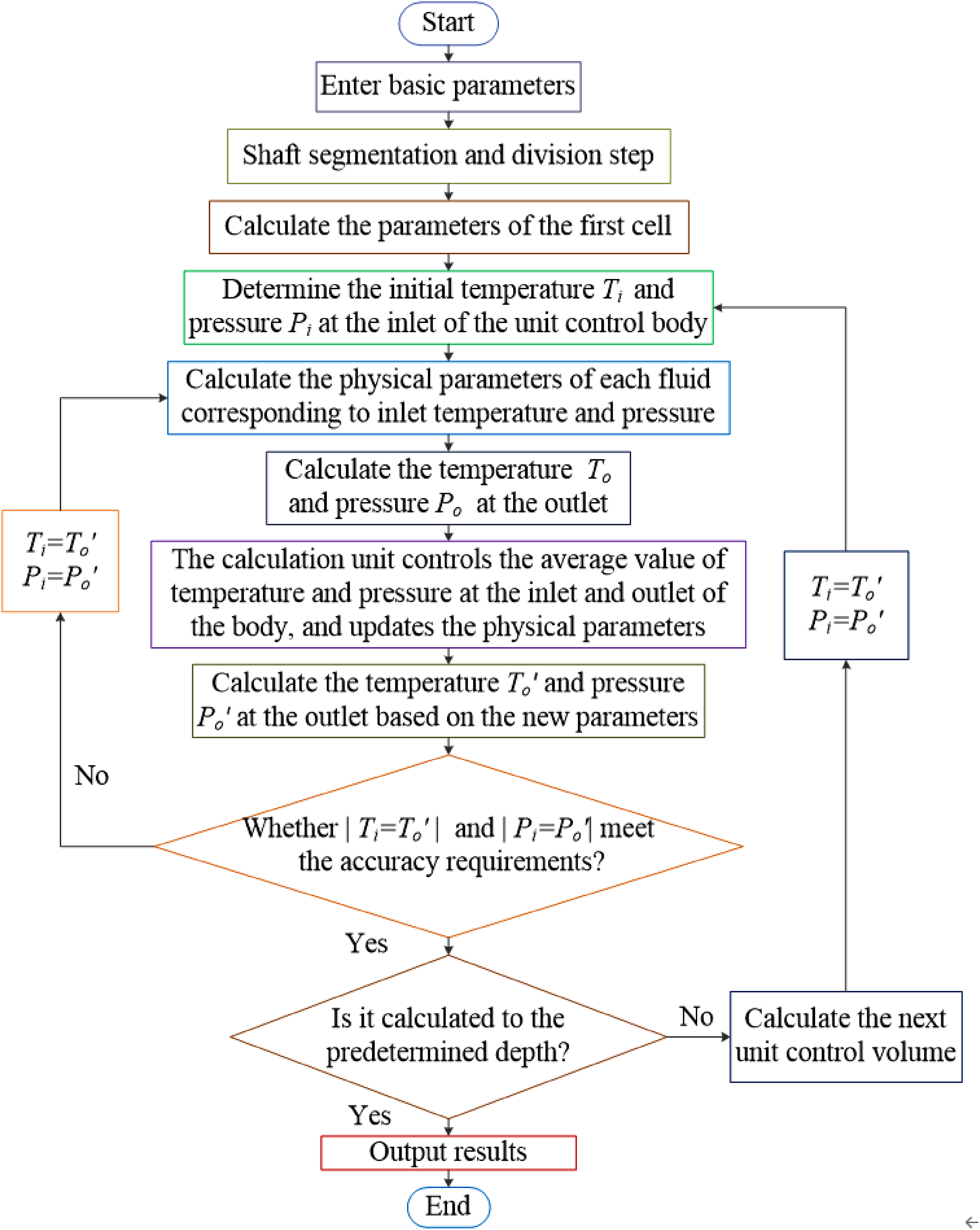
Temperature–pressure coupling calculation flow chart.
Example of temperature pressure coupling calculation of opening wellbore of HTHP gas well
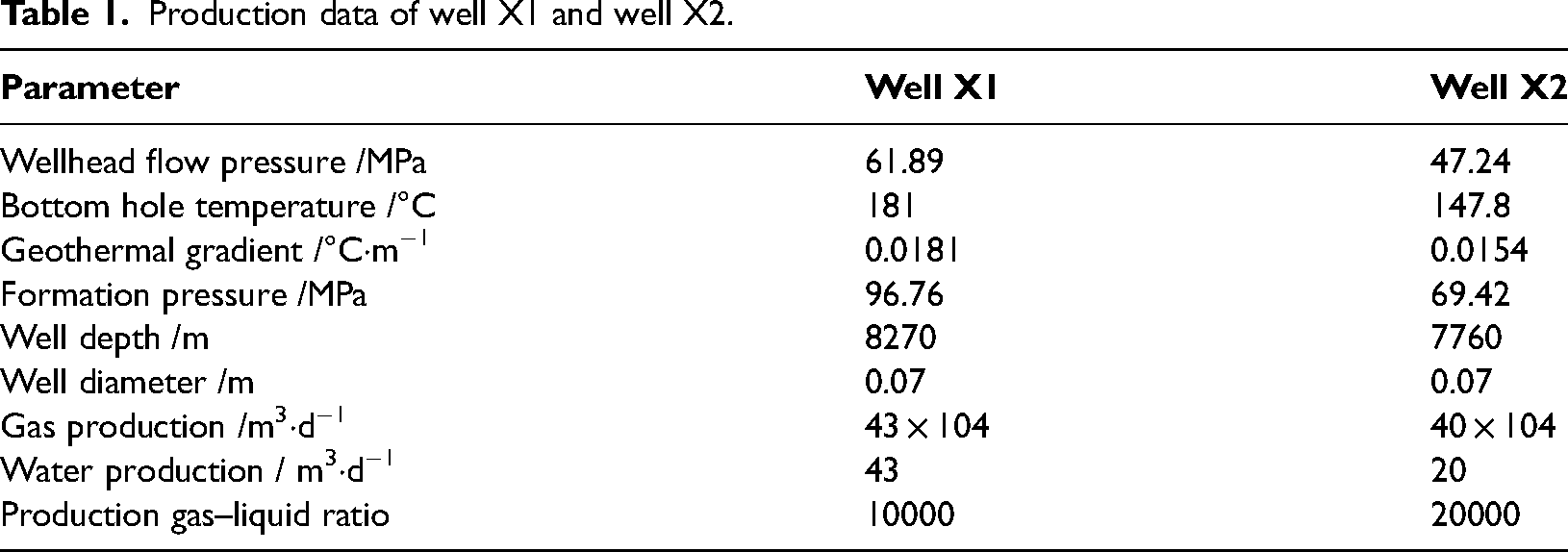
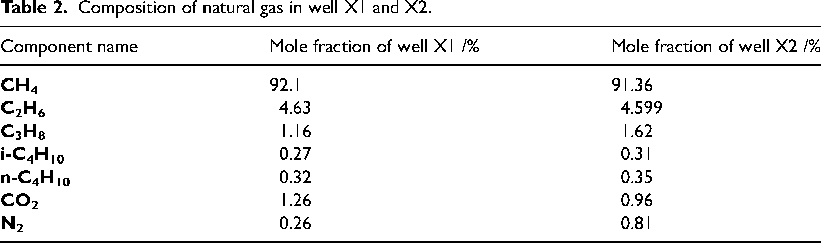
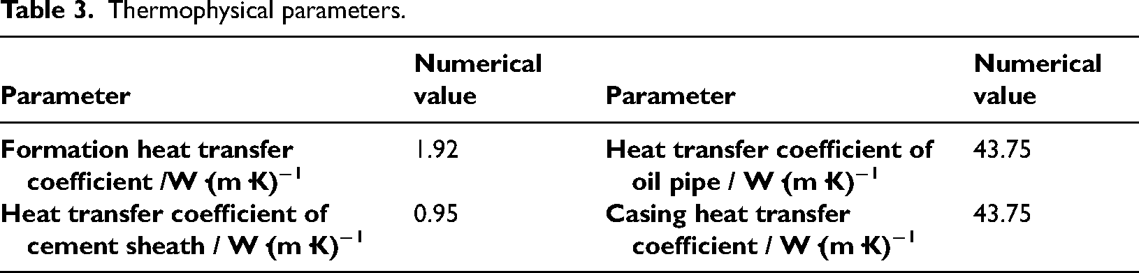
Fundamental data from X1 and X2, an actual well in a gas field, are used in the calculations and analysis. The relevant parameters for the two wells are shown in Tables 1, 2, and 3. Based on the coupling model of wellbore temperature and pressure established in this article, the sensitivity analysis of wellbore temperature and pressure is made by changing a certain condition of the gas well, and analyze the influence of different parameters on the temperature and pressure.
Production data of well X1 and well X2.
Composition of natural gas in well X1 and X2.
Thermophysical parameters.
The effects of various parameters on temperature and pressure are compared as follows:
The data in Figure 6 are 100 times the ratio of the change percentage of each parameter to the affected percentage of the result. It can be seen from the figure that gas well production and tubing size have a greater impact on the temperature and pressure variations, but the effects of gas–water ratio and heat transfer coefficient cannot be ignored.
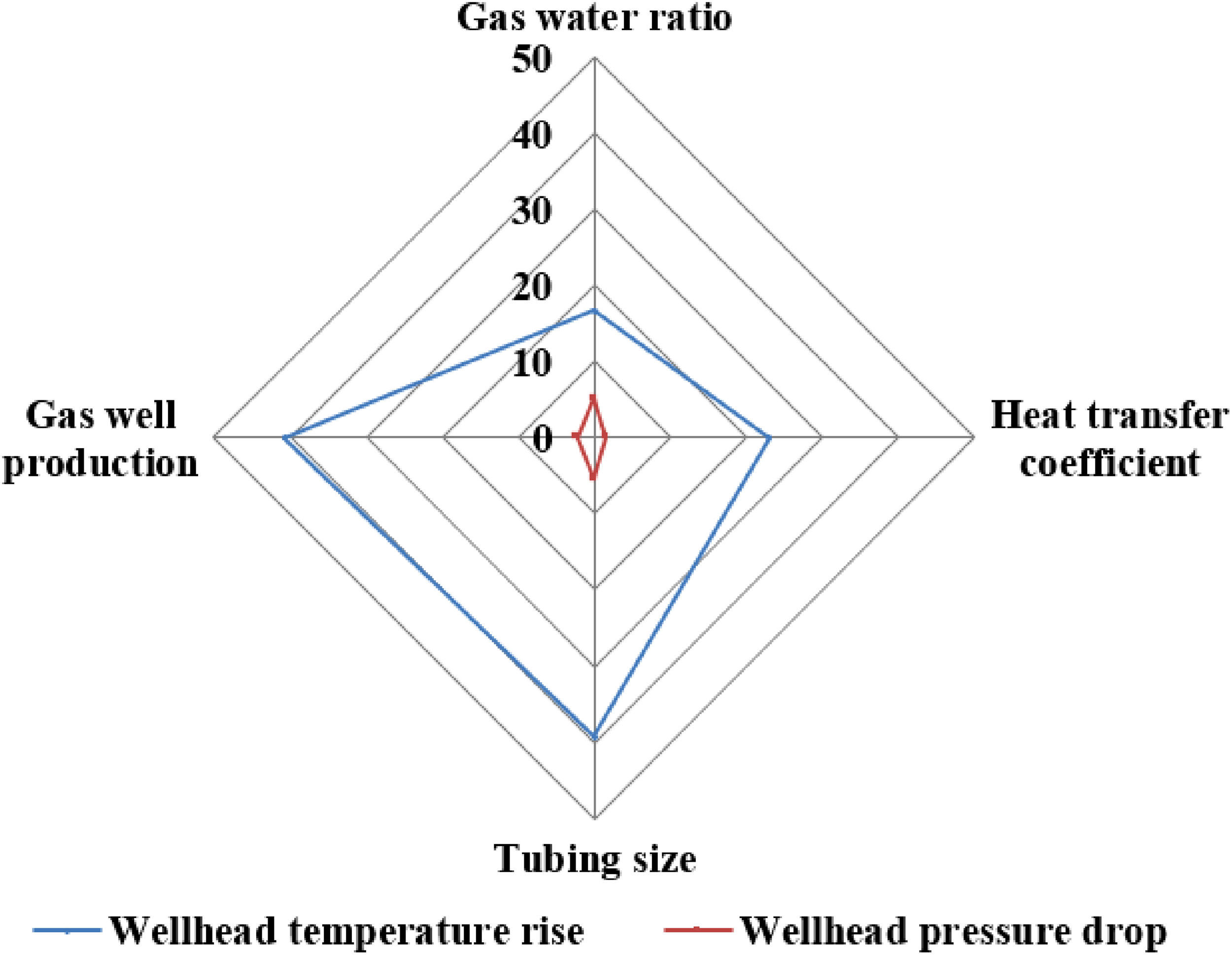
Schematic diagram of the influence of various parameters on temperature and pressure during well opening.
Influence analysis of gas–water ratio
Keeping other parameters constant, we compare the wellbore dynamical characteristics corresponding to different gas–water ratios. The corresponding wellbore temperature and pressure profiles were calculated at 0.5, 1, and 2 times the original gas–water ratio, respectively. The calculation results are shown in Figures 7 and 8.
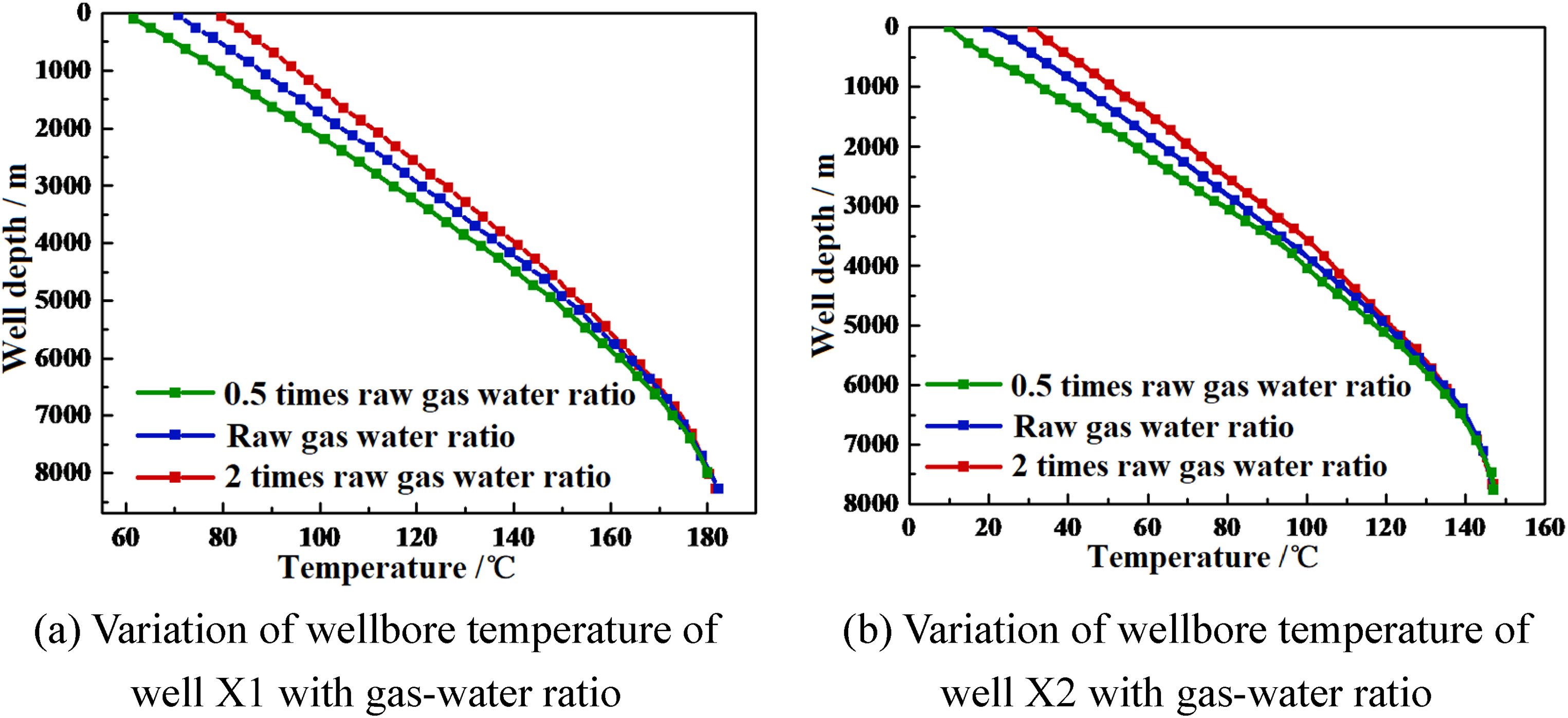
Variation of wellbore temperature profile with gas–water ratio.

Variation of wellbore pressure profile with gas–water ratio.
It can be seen from Figures 7 and 8, changes in the gas–water ratio have an impact on the distribution of wellbore temperature and pressure. When the gas–water ratio increases, the wellhead temperature gradually decreases. This is because the heat transfer capacity of water is stronger than that of natural gas fluid, and an increase in gas phase component will reduce the heat transfer capacity of the fluid in the wellbore. At the same time, an increase in the gas–water ratio, which is due to the compressibility of the gas itself, will also contribute to an increase in the wellhead pressure. When the proportion of gas phase increases, the wellbore pressure gradually increases. Therefore, the gas–water ratio of the gas well can be appropriately changed to adjust the wellhead pressure during the actual production process.
Influence analysis of heat transfer coefficient
The heat transfer coefficient is a very important parameter when predicting the wellbore temperature profile, which determines the rate of heat transfer between the wellbore and formation. Keeping other parameters constant during calculation, and calculate the corresponding wellbore temperature and pressure profile when the total heat transfer coefficient is 0.5, 1, and 2 times the original heat transfer coefficient, respectively. The results of calculation are shown in Figures 9 and 10.
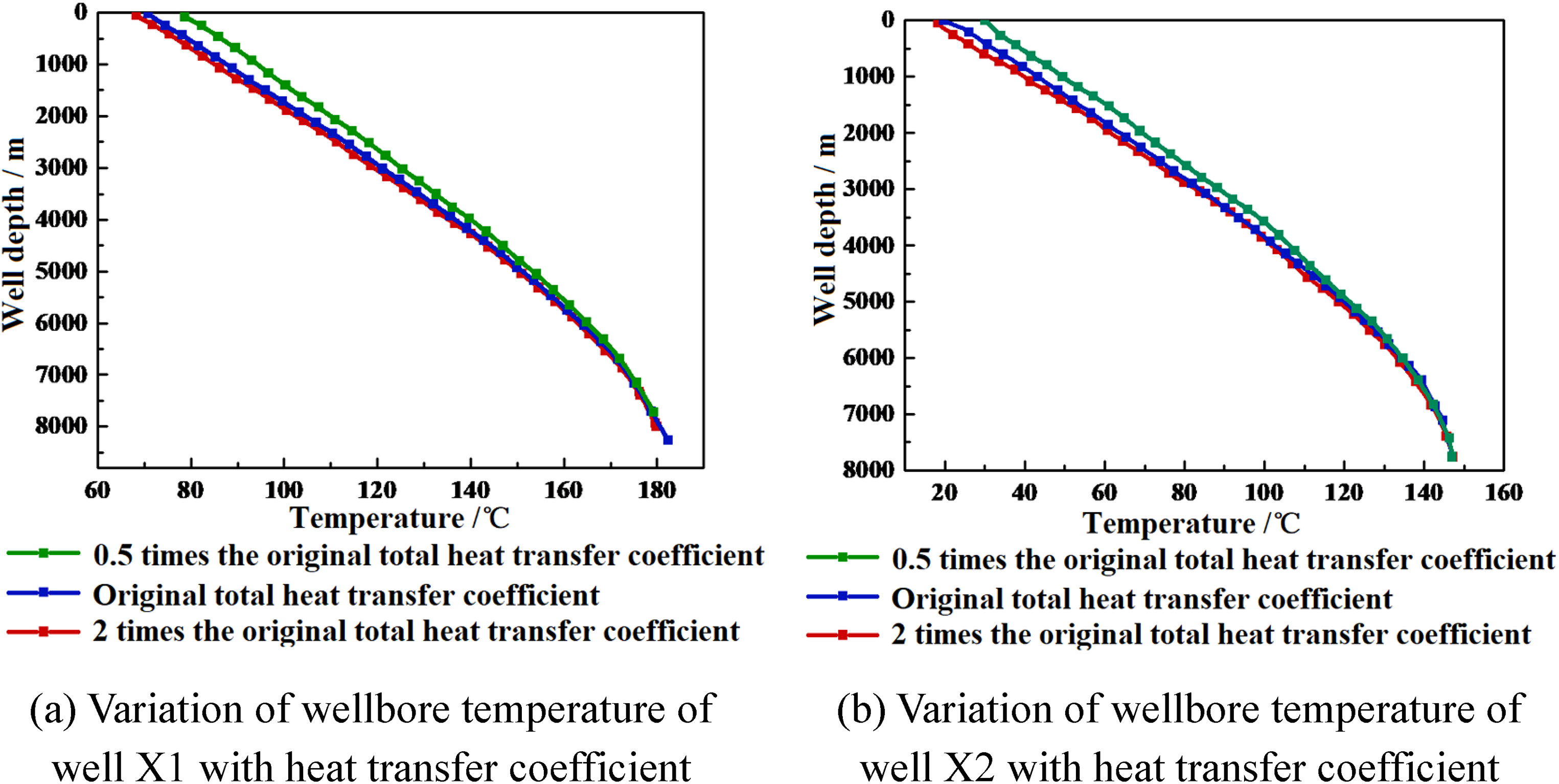
Variation of wellbore temperature profile with heat transfer coefficient.
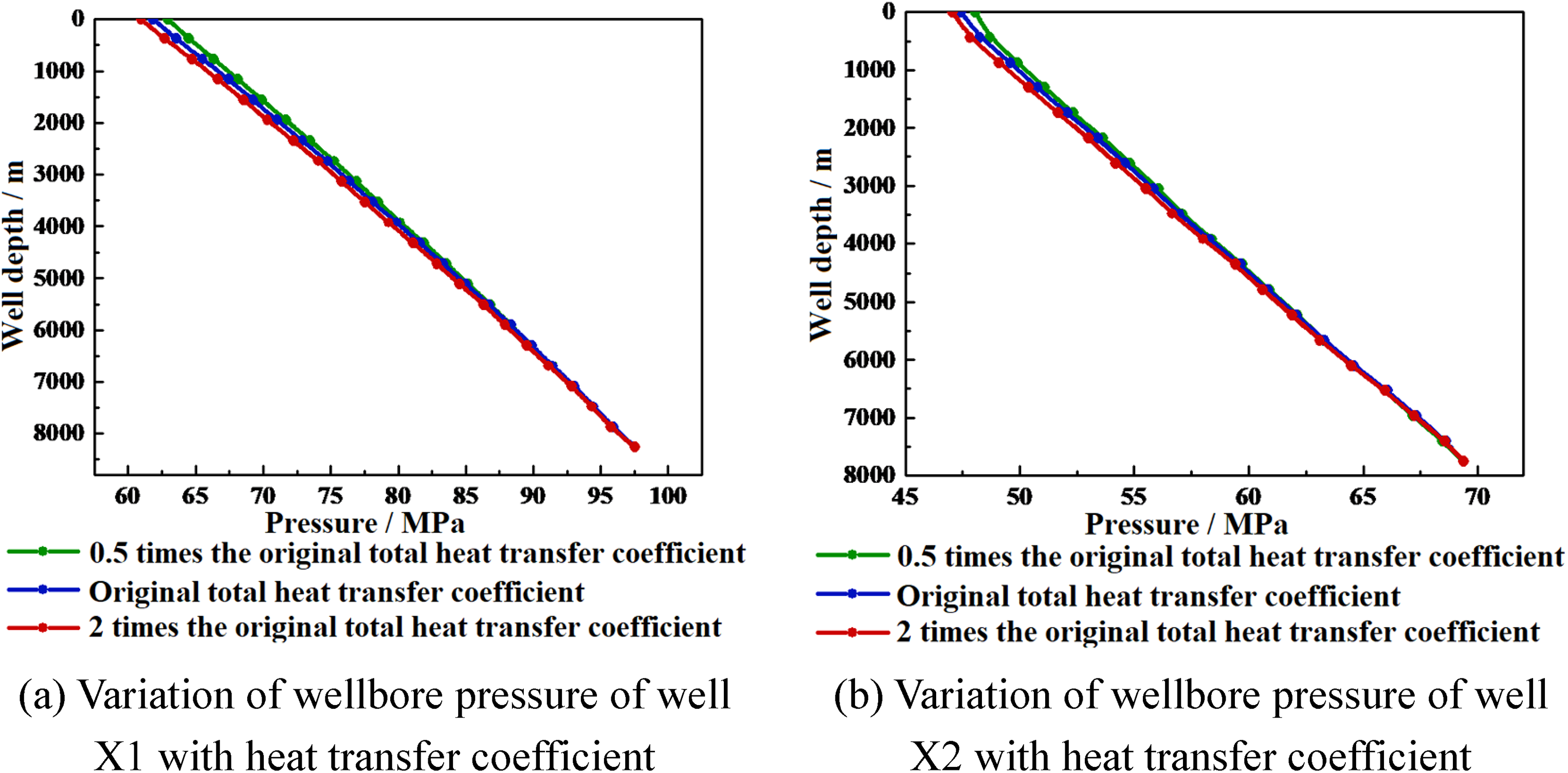
Variation of wellbore pressure profile with heat transfer coefficient.
It can be seen from Figures 9 and 10 that with the increase of the heat transfer coefficient, the wellhead temperature gradually decreases, and the change of the heat transfer coefficient has little impact on the pressure profile. This is because the larger the value of heat transfer coefficient, the faster the heat transfer between the wellbore and formation, which means that the heat loss in the process of heat transfer will gradually increase, resulting in a lower wellhead temperature.
Influence analysis of tubing size
In order to explore the influence of the change of tubing size on the wellbore temperature and pressure field, the wellbore temperature and pressure profile are calculated when the tubing size is 2 ⅞ inch, 3 ½ inch and 4 inches, respectively. The results of calculation are shown in Figures 11 and 12.
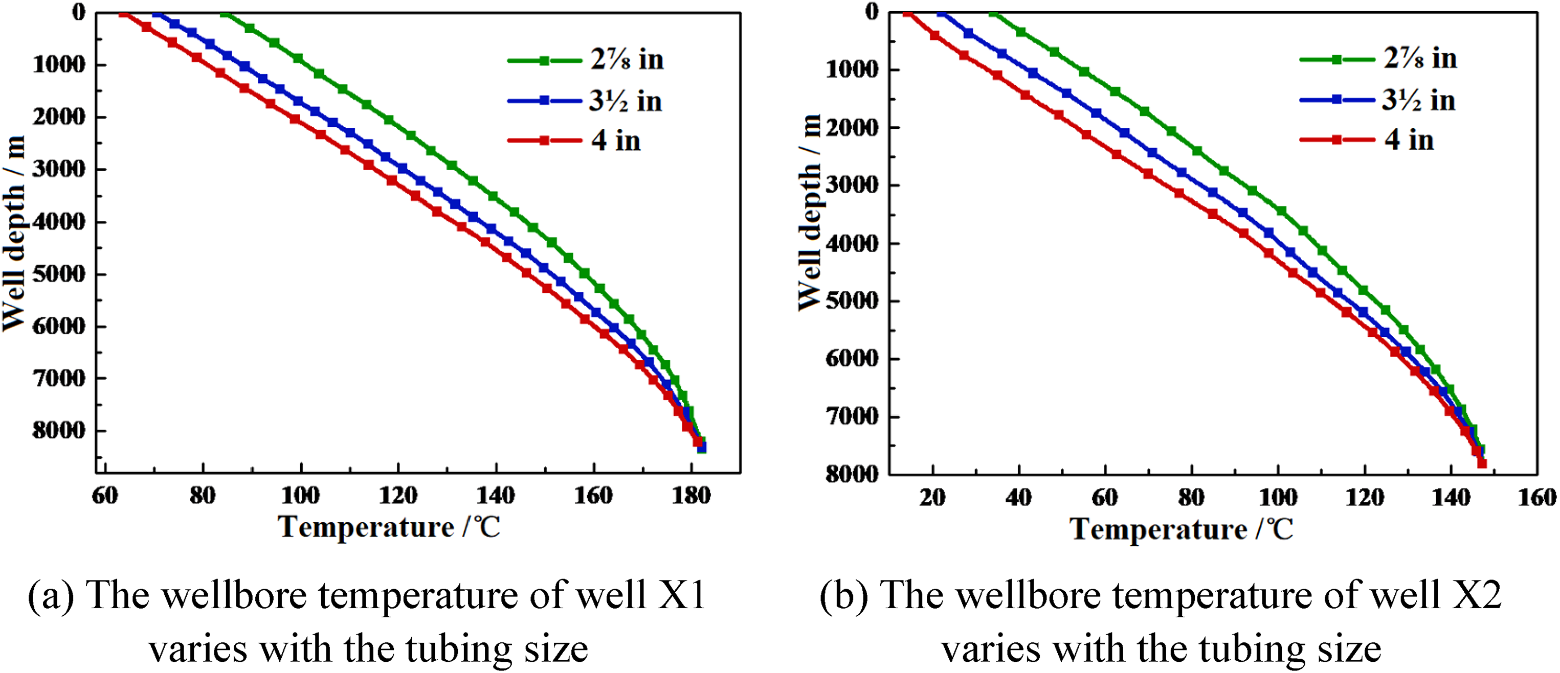
Variation of wellbore temperature profile with tubing size.
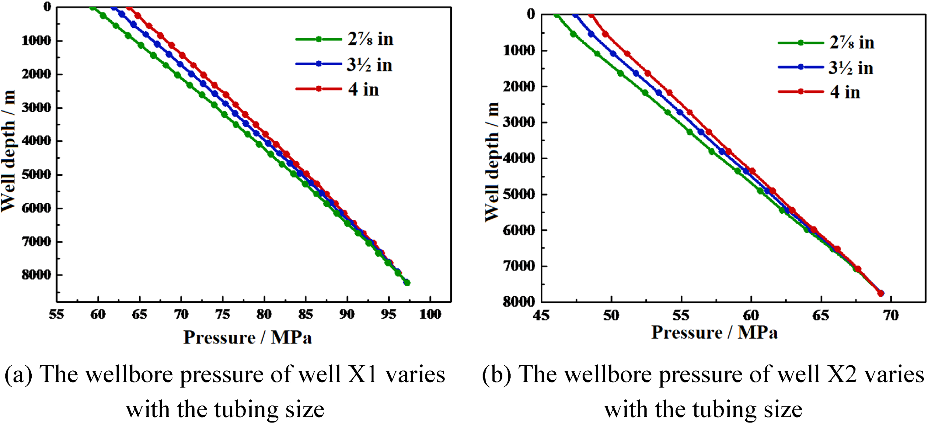
Variation of wellbore pressure profile with tubing size.
It can be concluded from Figures 10 and 11 that a change in tube size will have an impact on the wellbore temperature and pressure. As the tube size increases, the wellhead temperature gradually decreases and the wellhead pressure increases. The increase in tubing size will reduce the friction along the pipeline, so the convective heat transfer area of fluid in the pipeline increases, followed by a decrease in the wellhead temperature. At the same time, the increase in tubing size will also affect the decrease in fluid flow rate per unit area, and the wellhead pressure will gradually increase.
Impact analysis of gas well production
In order to explore the influence of gas well production on the wellbore temperature and pressure, the gas production was located at 0.5, 1, and 2 times of the original gas production and corresponding wellbore temperature and pressure profiles were calculated for the three cases. The calculation results are shown in Figures 13 and 14.
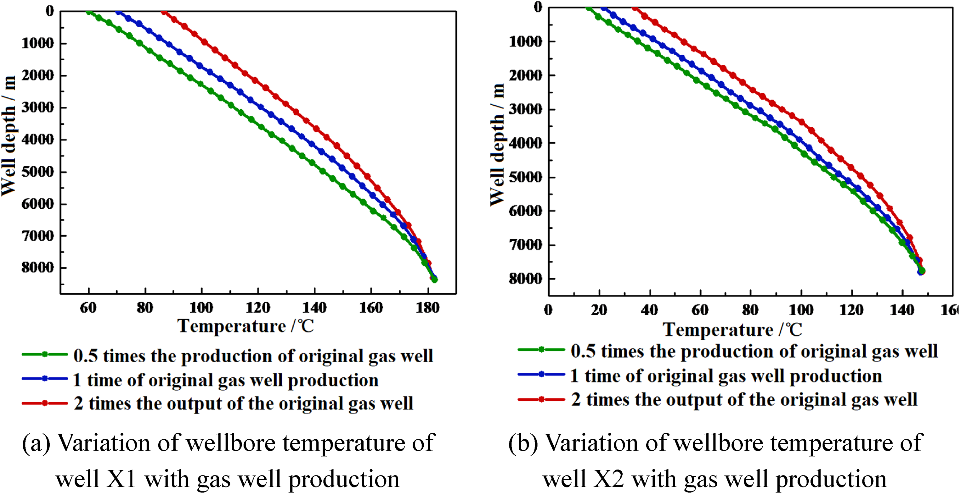
Variation of wellbore temperature profile with gas well production.
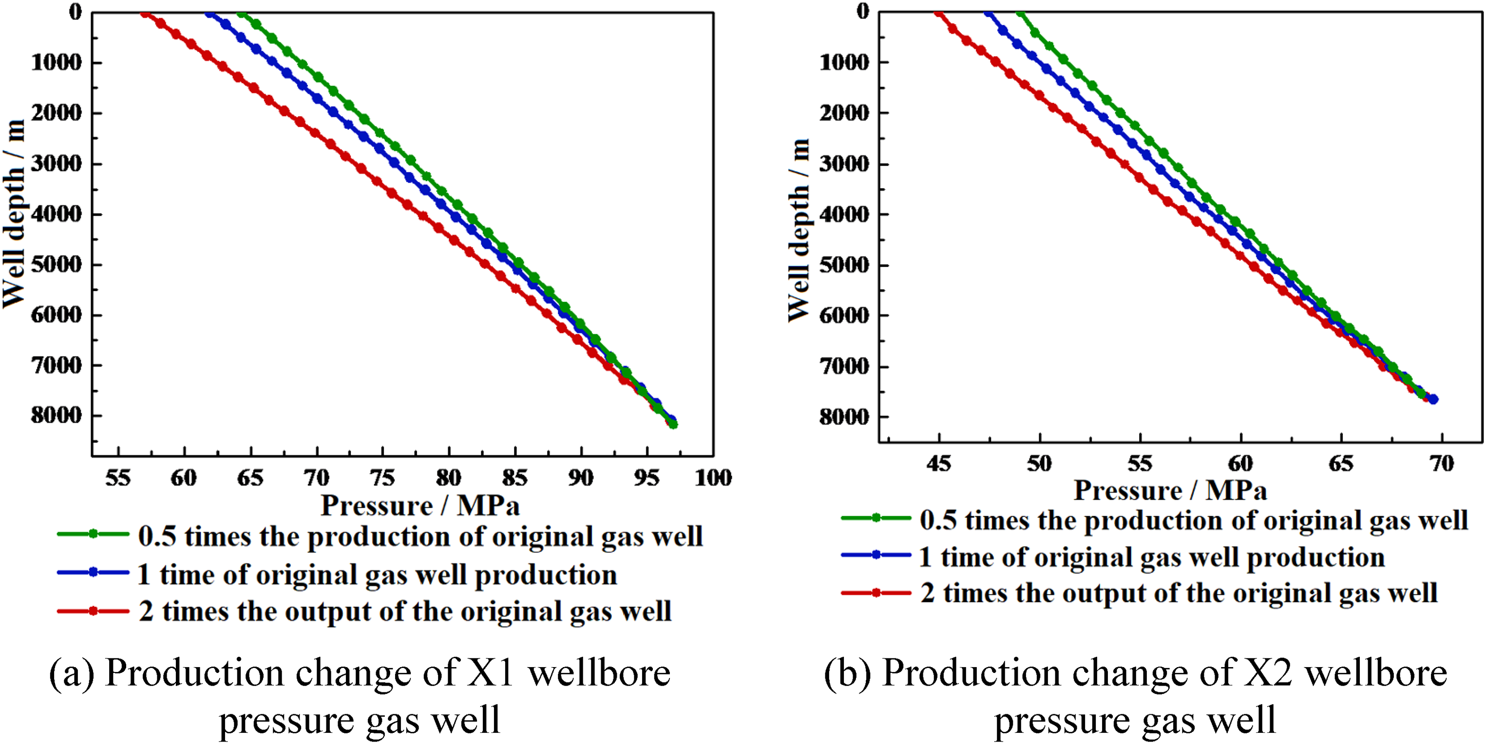
Variation of wellbore pressure profile with gas well production.
It can be seen from Figure 13 that the wellbore temperature increases with the increase in well depth. The corresponding temperature at any position in the wellbore increases with the increase of gas well production, and the temperature change range at the wellhead is the most obvious. This is because the increase in production is generally accompanied by the increase of fluid flow velocity in the wellbore, resulting in the increase of kinetic energy, the reduction of heat loss in the ring transfer process between the fluid and the surrounding environment, and the friction between the fluid and the wellbore will also produce some heat. As can be seen from Figure 14, when gas well production increases, the pressure at the same depth of the wellbore decrease. This is mainly because when the production increases, fluid and pipe wall resistance in the wellbore will also increase. In order to overcome the resistance, energy needs to be consumed, resulting in a rapid increase in the friction pressure drop and a decrease in the wellbore pressure. Therefore, it can be concluded that the wellbore temperature and pressure are affected by the gas well production.
Example of temperature pressure coupling calculation of shut-in wellbore of HTHP gas well
Using the shut-in wellbore temperature and pressure prediction model established in this article, we predict and analyze the temperature and pressure distribution in the wellbore of X1 and X2 wells.
Analysis of temperature and pressure calculation results
According to the calculation method of wellbore temperature and pressure, the temperature and pressure distribution of HTHP gas wells during well shut-in is calculated and analyzed. Figure 15 shows the wellbore temperature distribution under different shut-in times based on the wellbore temperature calculation model after shut-in.
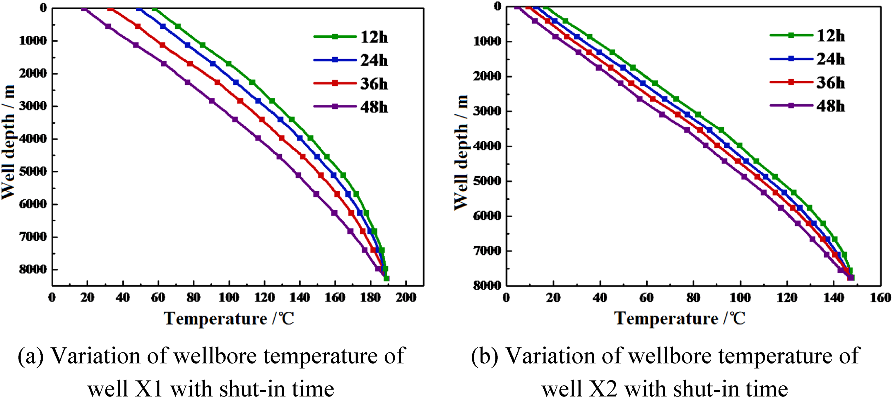
Wellbore temperature distribution corresponding to different shut-in time.
It can be seen from Figure 15, the change of wellbore temperature with well depth is nonlinear after a period of shut-in. When the well depth increases, the wellbore temperature gradually decreases and the temperature change rate gradually decreases. With the continuous increase of shut-in time, the corresponding temperature at the same position in the wellbore gradually decreases. This is because the fact that the fluid in the tube is in a nonflowing state after shut-in. With the continuous extension of time, the heat loss increases, resulting in a continuous decrease of wellbore temperature. It can be predicted the shut-in time is extended indefinitely, the heat transfer between the wellbore and the formation will be in a stable state, and the influence of the surrounding environment on the temperature can be neglected.
Figure 16 is a schematic diagram of the variation of wellhead and bottom-hole pressure with shut-in time after simulating the whole process of shut-in after a period of stable production of gas wells.
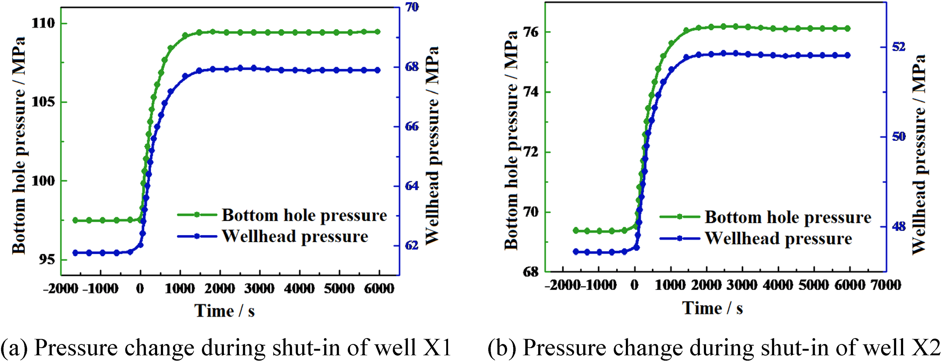
Variation of wellhead and bottom hole pressure with shut-in time.
It can be seen from Figure 16, the pressure at the wellhead and bottom increases continuously until it is stable after well shut-in. The pressure growth rate is large during the initial stage of well shut-in, and the growth rate gradually slows down with the increase of well shut-in time. When the pressure increases to a certain range, there will be no significant change. If the shut-in time is extended indefinitely, the wellbore temperature will be in equilibrium with the formation temperature, and the temperature will no longer have an impact on the pressure.
Temperature and pressure sensitivity analysis
The effects of various parameters on pressure are compared:
The value in Figure 17 is 100 times the ratio of the percentage of the wellhead pressure rise to the percentage of the parameter adjustment. It can be seen from Figure 18 that the tube size has a very significant effect on the inlet pressure.
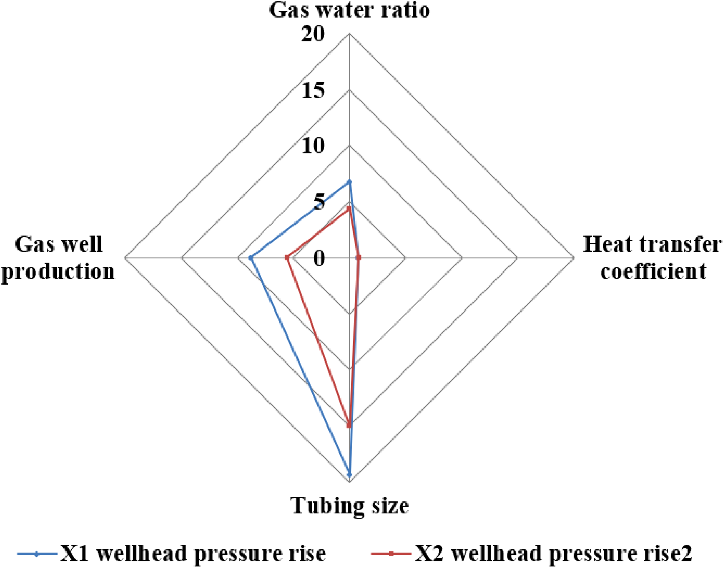
Schematic diagram of the influence of various parameters on temperature and pressure during well opening.
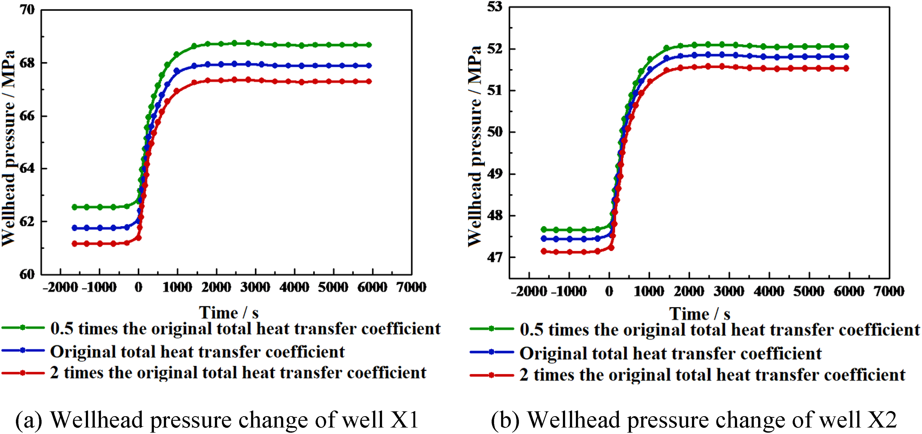
Simultaneous interpreting of wellhead pressure and shut-in time with different heat transfer coefficients.
Influence analysis of gas–water ratio
The change in wellhead pressure corresponding to the shut-in of well after one period of gas production was calculated for 0.5, 1, and 2 times the original gas–water ratio, respectively. The calculation results are shown in Figure 19.
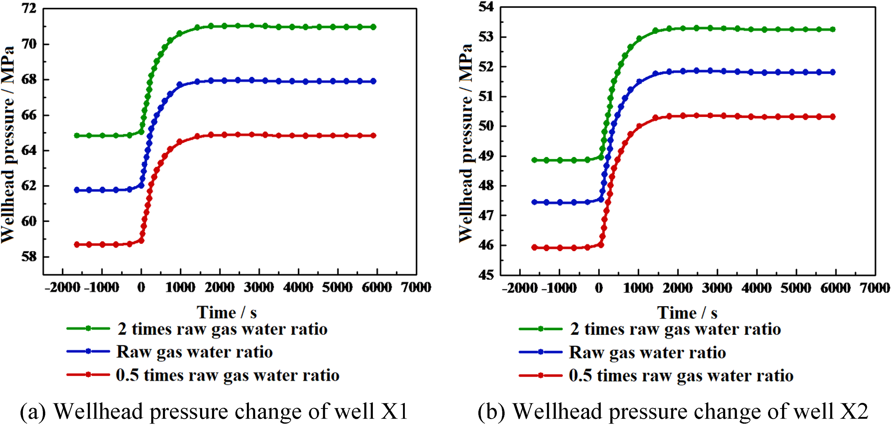
Variation of wellhead pressure corresponding to different gas–water ratio with shut-in time.
It can be seen from the figure that the wellhead pressure increases gradually under the recovery of formation pressure. With the increase of gas–water ratio, so does the wellhead pressure of the gas well, both before and after well is shut-in. The wellhead pressure changes rapidly during the initial stage of well shut-in and tends to stabilize over time. The increase in the gas–water ratio means that the proportion of liquid phase decreases, and the decrease of liquid content will slow down the situation that the upper component of fluid components in the wellbore is light and the lower component is heavy, resulting in the wellhead pressure affected by the change of gas–water ratio.
Influence analysis of heat transfer coefficient
The change in pressure at the wellhead corresponding to the shut-in of the gas well after a period of stable production was calculated for 0.5 times the total heat transfer coefficient, 1 time and 2 times the original heat transfer coefficient. The calculation results are shown in Figure 18.
It can be seen from Figure 18, the wellhead pressure as a whole shows an upward trend, and the increase in the heat transfer coefficient leads to a relative decrease in the corresponding wellhead pressure, but the effect is not great. Because the change in the heat transfer coefficient affects the unsteady heat conduction process, which then affects the temperature profile, the fluid temperature after shut-in will not have a great impact on the wellhead pressure, which is also verified by the calculations.
Influence analysis of tubing size
Keep other parameters unchanged, and calculate the wellhead pressure change corresponding to shut-in after a period of well opening and production when the tubing sizes are 2 ⅞, 3 ½, and 4 inches, respectively. The calculation results are shown in Figure 20.
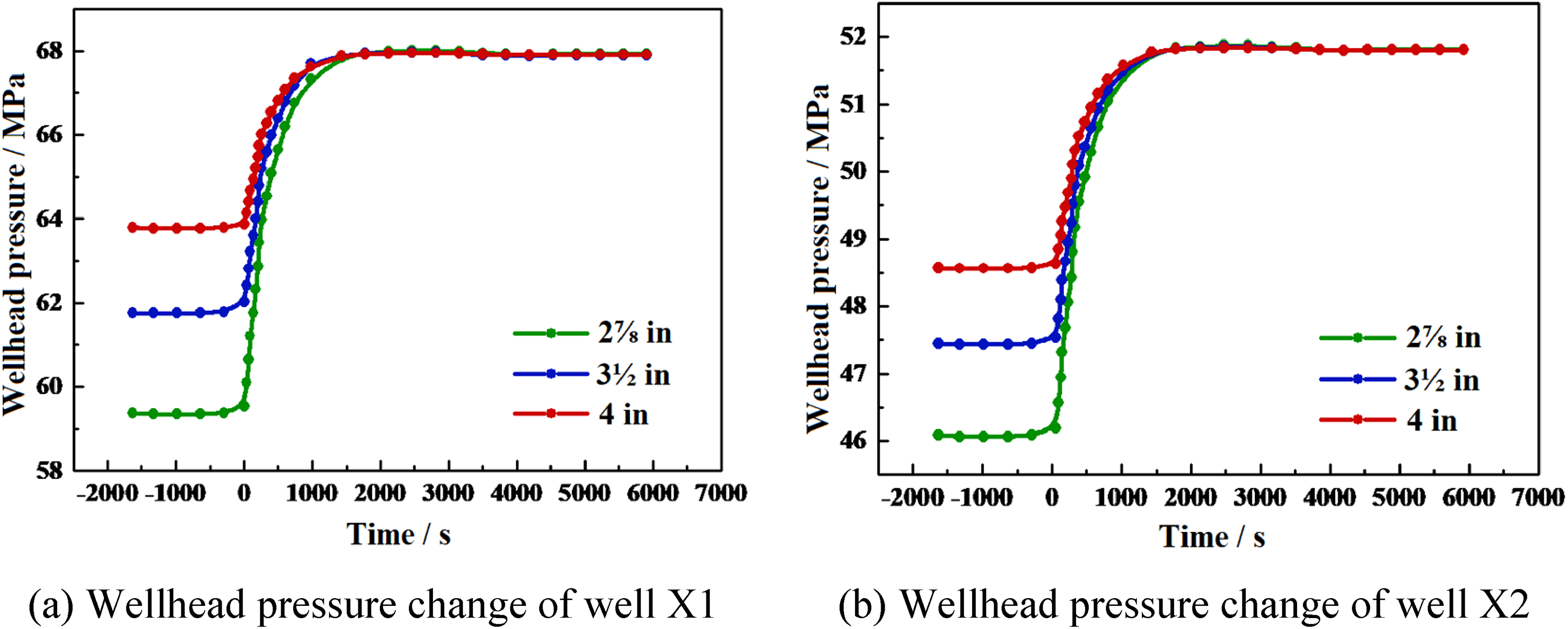
Variation of wellhead pressure corresponding to different gas well production with tubing size.
It can be seen from Figure 20 that the wellhead pressure increases with the tube size during stable production. No matter how large the tube size is, the corresponding wellhead pressure after shut-in gradually increases, and the wellhead pressure is basically stable at the same level after a period of time.
Impact analysis of gas well production
It can be seen from Figure 21 that the wellhead pressure before shut-in is affected by the gas well production. When production is increased, the corresponding wellhead pressure decreased. Different production corresponds to the wellhead pressure of the gas well after stable production. After being shut-in for a period of time, the wellhead pressure remained essentially at the same level.
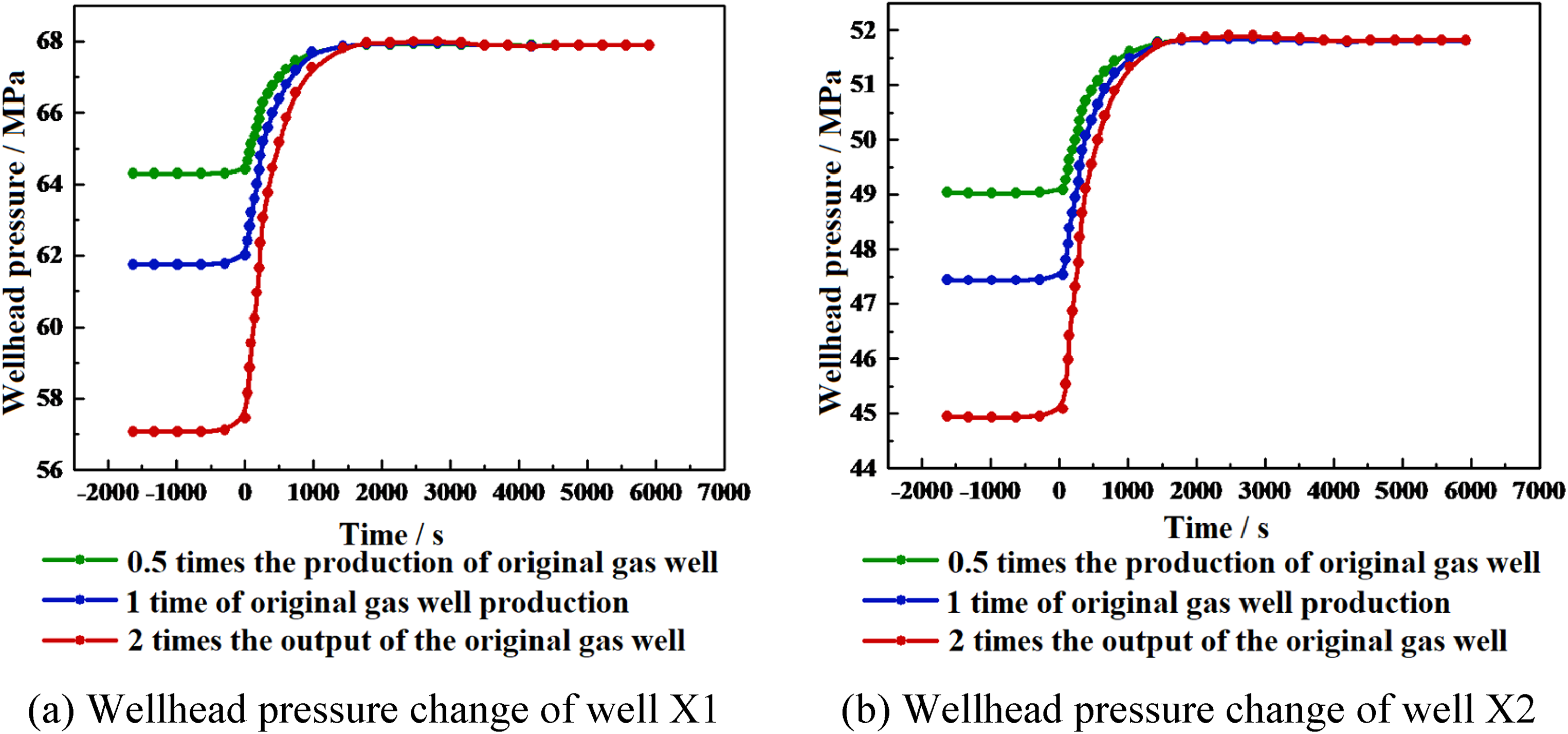
Variation of wellhead pressure corresponding to different gas well production with shut-in time.
Conclusion
Considering that the calculation of wellbore temperature and pressure can lead to large errors in the calculation results, an iterative algorithm is adopted for coupling the calculation of temperature, pressure and fluid physical parameters. The model established in this article was used to solve and calculate the wellbore temperature and pressure during the well opening and shut-in of two gas wells, thus validating the accuracy of the model. At the same time, the sensitivity analysis of wellbore temperature and pressure in the process of well opening and shut-in is carried out, and the influence of gas–water ratio, heat transfer coefficient, tubing size, gas well production, etc. on wellbore temperature and pressure profile in the process of well opening and closing is explored, and the reasons are further analyzed. Analysis found that:
Due to the interaction between temperature, pressure, and physical parameters, in order to improve the calculation accuracy of the model, it is necessary to select iterative algorithm to couple the temperature and pressure model. By comparing the established model with field well examples, it is concluded that the calculation results of the model in this paper are more accurate and the accuracy meets the actual requirements. The sensitivity analysis of wellbore temperature and pressure under the condition of well opening and well closing is carried out combined with well examples. It is found that when the gas–water ratio increases, the wellbore temperature decreases and the pressure increases; when the heat transfer coefficient increases, the wellbore temperature decreases and the pressure change is not obvious; when the tubing size increases, the wellbore temperature decreases and the pressure increases; when the gas well production increases, the wellbore temperature increases and the pressure decreases.
Footnotes
Nomenclatures
Data availability
The manuscript is a data self-contained article, whose results were obtained from the laboratory analysis, and the entire data are presented within the article.
Declaration of conflicting interests
The authors declared no potential conflicts of interest with respect to the research, authorship, and/or publication of this article.
Funding
The authors disclosed receipt of the following financial support for the research, authorship, and/or publication of this article: This project was supported by the National Natural Science Foundation of China (52004215, 12101482, 52374039, 52274006), Shaanxi Youth Science and Technology New Star Project (Talent) (2023KJXX-052), Gansu Province Technology Innovation Guidance Plan (23CXGL0018), Shaanxi Province Technology Innovation Guidance Plan (2024QCY-KXJ-019), the Key R&D Plan of Shaanxi Province (2022GY-129,2023-YBSF-372), China Postdoctoral Science Foundation(2022M722604), Shaanxi Provincial Market Regulation Science and Technology Plan Project (2022KY15, 2023KY14), Pingliang Special Plan for Scientific and Technological Talents (PL-STK-2022A-095).