A study on time-varying dependence between energy markets and linked assets based on the Russia-Ukraine conflict

Abstract

The energy industry, acutely sensitive to geopolitical shifts due to the Russia-Ukraine conflict, experiences sustained disturbances in global energy markets, reshaping global energy supply dynamics and significantly influencing global trade patterns. Utilizing static and dynamic GARCH-Copula models, this study elucidates the dependency between energy markets and related assets. The Copula function, when compared with the multivariate GARCH model, demonstrates distinct advantages, notably in delineating joint asset distributions, capturing market dependence's nonlinear traits, and highlighting robust tail correlation structures. Beyond the average inter-market dependence, its tail correlation offers a vital perspective on market risk. This research delves into the temporal and structural variations in interdependence between energy markets and related assets. It probes potential structural breakpoints in dynamic interdependence and pinpoints their occurrences. By focusing on the Russia-Ukraine conflict, this study offers a holistic view of the changing interplay between the energy market and other asset categories, providing pivotal insights for investor portfolio optimization, regulatory oversight, and risk mitigation. Moreover, employing wavelet analysis, this study examines the frequency domain traits of the interdependency between energy markets and associated assets. As frequency wanes, market price fluctuations become less pronounced. The continuous wavelet power spectrum indicates that price variations are predominantly mid to high frequency. Cross-wavelet transform results suggest that correlations between energy markets and related assets are more influenced by short-term perturbations than enduring shifts.

Preface

Russia stands as a predominant energy producer globally, supplying Europe with significant proportions of its energy needs—30% of its crude oil and 35% of its natural gas. Consequently, Europe exhibits a pronounced reliance on Russian energy resources. The geopolitical tensions stemming from Russia's military activities in Ukraine prompted stringent economic sanctions from the United States and the European Union. This, in turn, nudged Russia to recalibrate its energy strategies. Simultaneously, European nations have been fervently exploring alternative energy sources, leading to substantial shifts in the global energy paradigm. These geopolitical disturbances have escalated the risk of synchronized volatility in the energy financial markets. Notable indices, such as the Shanghai Stock Exchange and the Hang Seng Index, experienced pronounced declines. Concurrently, stock markets in the UK, France, and Germany also registered significant drops. This study illuminates the temporal characteristics of the interdependence between energy markets and related assets, considering both the degree and structure of this interrelation. Utilizing structural breakpoint analysis, it pinpoints key crisis events that induce alterations in interdependence structures. The findings underscore a positive, time-varying dependence between the energy market and its associated assets, save for the money market. Additionally, an asymmetric tail dependence in the energy market contrasts with the symmetric tail dependence observed in other markets.

Modeling

Construction of the Copula model

First introduced by Sklar in 1956, Copula functions, often referred to as conjugate functions, are renowned for their proficiency in detailing the correlation structure of random variables. These functions not only outline the nonlinear correlation architecture between markets but also unveil the tail correlation in extreme market scenarios, positioning them a notch above the traditional multivariate GARCH model.

Sklar's theorem posits that each Copula function (also termed a covariance function) can amalgamate the joint distribution of the variables with their individual marginal distributions. Let's presume the existence of a copula function abiding by:

$$F_{xy}(x,y)=C(F_x(x),F_y(y))$$

(1)

Where, and represent marginal distributions. For continuous is denoted as follows:

$$C(u,v)=F_{xy}(F^{-1}X(u),F^{-1}Y(v))$$

(2)

Where, both and (obtained via probabilistic integral transformation) uniformly range between [0,1], and signify the generalized inverse distribution functions of the marginals and $\mathrm{FY}$ , respectively.

In terms of dependence, the Copula function presents three pivotal advantages: First, it permits the individual modeling of marginal distributions, correlating their quantiles via the Copula function. This endows greater latitude in crafting marginal functions and correlations. Second, for non-elliptical joint distributions, the Copula function renders a more precise dependence metric, as the conventional dependence metric steered by the linear correlation coefficient fails to authentically capture the dependence blueprint. Third, it embraces tail dependence, quantifying the likelihood of simultaneous extreme ascents or descents in two variables. Joe (1997) meticulously defined the tail correlation coefficient as follows:

$${\tau }^U{=}_{u\uparrow 1}^{lim}P(x_1>F_{x_1}^{-1}(u)|x_2>F_{x_2}^{-1}(u))=\begin{array}{c}lim\\ u\uparrow 1\end{array}{\displaystyle \frac{1-2u+C(u,u)}{1-u}}$$

(3)

With the cap presented as follows:

$${\tau }^L{=}_{u\downarrow 0}^{lim}P(x_1\le F_{x_1}^{-1}(u)|x_2\le F_{x_2}^{-1}(u))=\begin{array}{c}lim\\ u\uparrow 1\end{array}{\displaystyle \frac{C(u,u)}{u}}$$

(4)

Where, ${\tau }^U,{\tau }^L\in [0,1]$ denotes upper and lower tail dependences. A scenario where signifies the absence of tail dependency.

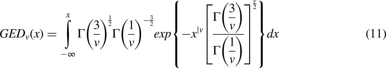
Copula functions manifest in an array of forms. To meticulously delineate the dependence framework between the energy market and interlinked assets, this study employs common Archimedean and elliptical class Copula functions, each exhibiting distinct tail characteristics. The optimal fit connection function model is then harnessed to further gauge the CoVaR.

The two-stage stepwise estimation method, known as the iterated filtering method, is employed in this study to deduce the relevant parameters. The steps are detailed below: Initially, all parameters in the marginal distribution functions for both the energy market and linked asset return series, fitted via the ARMA(p, q)-GARCH(1,1) model, are determined. The estimated values of these parameters are represented as follows:

$${\theta }^i=argmax\sum _{t=1}^{T}ln{f}_t^i(R_t^i;{\theta }^i),i=GB,S$$

(5)

Where, T represents the sample size, $f_t^i(\cdot )$ represents the density function of the marginal distribution, GB represents the energy market, and S represents the associated assets.

Similarly, all parameters ${\theta }_C$ in the Copula model can be obtained and estimated as follows:

$${\theta }^i=argmax\sum _{t=1}^{T}ln{c}_t(F_S{R}_t^S;{\hat{\theta }}^S),F_{GB}(R_t^{GB};{\hat{\theta }}^{GB});{\theta }_C$$

(6)

Where, $C_t(\therefore )$ signifies the density function of the Copula model.

Finally, in this paper, Akaike's information criterion (AIC) is standardized for an assortment of models, written by the following expression:

$$AIC=2k-2\sum _{t=1}^{T}ln{c}_t(F_S(R_t^S;{\hat{\theta }}^S),F_{GB}(R_t^{GB};{\hat{\theta }}^{GB});{\hat{\theta }}_C){\theta }_C$$

(7)

Where, k represents the total number of model parameters. A lesser AIC value indicates superior model accuracy. Thus, the time-varying Copula model with the minimal AIC value is distinguished as the optimal one.

The marginal distribution models of energy market and correlated asset returns R $t(S)$ are identified as ARMA with Generalized Autoregressive Conditional Heteroskedasticity errors. Specifically, these models are the ARMA(p, q)-GARCH(1,1) variants steered by a generalized error distribution (GED) which astutely captures salient features of the energy market R $t(GB)$ and the correlated asset returns R $t(S)$ , such as pronounced tails, leverage effects, and conditional heteroskedasticity. The mean equation is represented by the ensuing ARMA(p, q) process:

$$R_t^i={\phi }_0+\sum _{j=1}^p{\phi }_0{R}_{t-j}^i+{\epsilon }_t^i+\sum _{j=1}^p{\theta }_j{\epsilon }_{j-1}^i={\mu }_t^i+{\epsilon }_t^i,i=GB,S$$

(8)

Where, both p and q represent non-negative integers. ${\epsilon }_t^i={\sigma }_t^i{z}_t^i$ , where $z_t^i$ adheres to an independent GED distribution with degrees of freedom ν and ${\sigma }_t^i$ conditional standard deviation, aligning with the variance equation articulated in (4.9):

$${\sigma }_t^{i^2}=\omega +a_1{\epsilon }_{t-1}^{i^2}+{\beta }_1{\sigma }_{t-1}^{i^2}$$

(9)

Where, the parameters $\omega ,a_1,{\beta }_1$ , and $\mathrm{v}$ require estimation, and for series stability, and $a_1$ and ${\beta }_1$ must ensure $a_1+{\beta }_1<1$ . Leveraging the maximum likelihood estimation method, the marginal return distribution function for both the energy market and the associated assets is acquired as follows:

$$F^i(R_t^i)=P({\epsilon }_t^i\le R_t^i-{\mu }_t^i)=p\left(Z_t^i\le {\displaystyle \frac{R_t^i-{\mu }_t^i}{{\sigma }_t^i}}\right)=GE{D}_v\left({\displaystyle \frac{R_t^i-{\mu }_t^i}{{\sigma }_t^i}}\right)$$

(10)

Where, $GE{D}_v(\cdot )$ represents the distribution function of the GED, detailed as follows:

$$GE{D}_v(x)=\underset{-\mathrm{\infty }}{\overset{x}{\int }}\mathrm{\Gamma }{\left({\displaystyle \frac{3}{v}}\right)}^{\frac{1}{2}}\mathrm{\Gamma }{\left({\displaystyle \frac{1}{v}}\right)}^{-\frac{3}{2}}exp\left\{-x^{|v}{\left[{\displaystyle \frac{\mathrm{\Gamma }\left({\displaystyle \frac{3}{v}}\right)}{\mathrm{\Gamma }\left({\displaystyle \frac{1}{v}}\right)}}\right]}^{\frac{v}{2}}\right\}dx$$

(11)

Structural break detection

In contemporary research, two prominent methods exist for pinpointing structural breaks: First. Subjective Inference Method: This approach relies on visual analysis of time series plots to discern inflection points. By correlating these points with significant events occurring near them, researchers can hypothesize potential structural breaks. However, this method struggles to ascertain a direct sequence between inflection points and related events, potentially leading to flawed conclusions. Second, Financial Econometric Models: Techniques like the Chow and Cusum tests are employed to determine structural breaks. Nonetheless, these tests are not devoid of limitations. For one, the selection of sample intervals carries an inherent subjectivity, which risks misidentifying breakpoints. More critically, tests like Chow and Cusum can only evaluate a single breakpoint at a given time, restricting their applicability. Recognizing these limitations, this paper leverages the endogenous multiple breakpoint detection method, known as the BP test, as proposed by Bai and Perron (2003). This advanced technique surmounts the constraints of previous methods that were confined to single breakpoint assessments. Currently, the BP test stands out as a more precise and effective methodology. Under the BP test framework, the initial step is to structure a multivariate linear regression model, accounting for the breakpoints:

$$\begin{array}{c}{y}_t=x_t^{\mathrm{\prime }}\beta +z_t^{\mathrm{\prime }}{\delta }_{j+1}+{\mu }_t\\ t=T_j+1,T_j+2,\cdots ,T_j;j=1,2,\cdots ,m+1\end{array}$$

(12)

Where, $y_t$ is the dependent variable, $x_t,z_t$ is the independent variable, and $\beta ,{\delta }_{\mathrm{j}}$ is the corresponding vector of coefficients. ${\mu }_t$ denotes the residual term, $\mathrm{m}$ signifies the number of structural changes, and $\mathrm{T}1,\mathrm{T}2,\dots ,\mathrm{Tm}$ denotes the latest identified structural change point. $u_t$ represents white noise. The structural breakpoints can be derived by minimizing the sum of squares of the total residuals, i.e.:

$$({\hat{T}}_1,\cdots ,{\hat{T}}_m,{\hat{\delta }}_1,\cdots ,{\delta }_{m+1}^{\mathrm{\Lambda }})=argmi{n}_{T_1,\cdots ,T_m,{\delta }_1,\cdots ,{\delta }_{m+1}}{S}_T(T_1,\cdots ,T_m,{\delta }_1,\cdots ,{\delta }_{m+1})$$

(13)

Where, $S_T(T_1,\cdots ,T_m,{\delta }_1,\cdots ,{\delta }_{m+1})=\sum _{i=1}^{m+1}\sum _{k=T_{i-1}+1}^{T_i}(p_t-{\delta }_k{)}^2,T_0=0$

The procedure to determine structural breaks encompasses the following steps: Firstly, application of Fisher's Algorithm (1958): Equation (13) undergoes iterative processing using Fisher's algorithm to pinpoint the minimal value for the total residual sum of squares. Secondly, utilization of the supWald Test: This test facilitates the identification of the number of breakpoints and pinpoints their respective occurrence times.

The multiple structural breakpoint test is instrumental in delving deeper into the intertwined relationship between the energy market index and its related assets. By testing for shifts in the time-varying correlation coefficient, this methodology evaluates whether the interplay between the energy market and its associated assets undergoes structural changes. Recognizing these breakpoints and juxtaposing them with real-world events illuminates the tangible factors and significant occurrences that sway the interconnectedness of the energy market and related sectors. By synthesizing qualitative and quantitative analyses, researchers can pinpoint the precise moments of time-varying correlation shifts. This, in turn, aids in extrapolating the deterministic external events that precipitate extreme risks, offering invaluable insights for adeptly navigating the perilous waters of the energy market.

Data selection and processing

Energy market index selection

To track the performance of energy market returns, various indices denominated in different currencies have been developed. These are designed to encapsulate the price dynamics of energy commodities traded across different platforms. This study zeroes in on three global energy market indices: the Standard & Poor's Dow Jones Energy Market Index, the Bloomberg Barclays MSCI Energy Market Index (MSCI_GB), and the Solactive Energy Market Index. The objective is to juxtapose their price dynamics and volatility trajectories. Each of these indices employs a unique calculation methodology and has distinct components. Their usage is well documented in earlier research. Daily price data for these indices, spanning from 24 February 2022 to 24 December 2022, was sourced from the Bloomberg database. We derived the daily return series for these indices utilizing the percentage logarithmic difference approach. Table 1 delineates the descriptive statistics for the daily returns, noting an average return proximate to zero. Based on the Jarque-Bera test, the normality assumption for all three indices is rejected at a 1% significance level. These series exhibit analogous statistical attributes regarding mean, kurtosis, skewness, and normality. Furthermore, their Pearson correlation coefficients are elevated, especially between GB and MSCI_GB, which approach unity. It's evident that these energy market index series convey congruent market insights. Hence, owing to its precedence in publication, the S&P Dow Jones Energy Market Index (GB) is chosen as the emblematic energy market index for this paper.

Table 1.

Descriptive statistics of energy market indices.

	GB	MSCI_GB	SOLACTIVE_GB
Mean	0.0001	0.0001	0.0001
Median	0.0001	0.0001	0.0002
Maximum	0.0201	0.0220	0.0134
Minimum	−0.0241	−0.0303	−0.0182
Std.Dev.	0.0032	0.0037	0.0027
Skewness	−0.561	−0.575	−0.535
Kurtosis	8.756	8.916	7.166
Jarque-Bera	2285.565	2413.995	1207.973
Probability	0.0000	0.0000	0.0000
ADF	−24.9575	−36.9572	−35.5506
Pearson Correlation Coefficient
GB	1.000
MSCI_GB	0.996	1.000
SOLACTIVE_GB	0.778	0.787	1.000

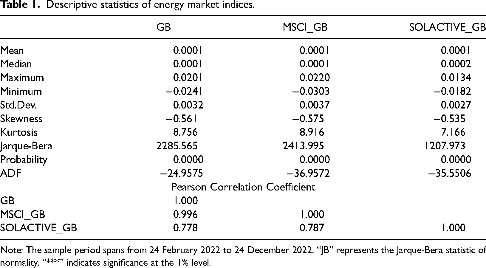
Note: The sample period spans from 24 February 2022 to 24 December 2022. “JB” represents the Jarque-Bera statistic of normality. “***” indicates significance at the 1% level.

Sample selection of linked assets

To investigate the interdependence magnitude and structure between the energy market and various other markets, this study considers traditional asset classes, including fixed income, equities, and energy commodity markets. Additionally, energy equity indices across diverse sectors are taken into account. Specifically, various clean energy industry indices from the NASDAQ OMX Energy Economics series are evaluated to assess the financial dynamics of the global energy equity market at an industry-specific level. This index series captures a breadth of sectors, representing the behavior of distinct energy stock sub-sectors, thus offering an expansive view of market trends within the energy domain. To ensure data consistency between the energy market and the energy industry stock, we primarily focus on indices from the NASDAQ OMX Energy Economics series that have significant relevance to energy market trends.

Therefore, guided by the work of Ferrer et al. (2021), this paper selects indices related to solar (GRNSOLAR), wind (GRNWIND), natural gas (GRNFUEL), energy efficiency (GRNENEF), clean transportation (GRNTRN), energy-centric buildings (GRNGB), pollution prevention (GRNPOL), and water management (GRNWATER). Among these, the GRNSOLAR and GRNWIND indices are curated to reflect the performance of enterprises engaged in energy production via solar and wind modalities, while the GRNFUEL index encompasses firms involved in natural gas-based energy production.

Table 2 presents the principal descriptive statistics concerning the daily returns of all time series throughout the sample period. The table indicates that the mean values of daily returns for all variables approximate zero and are notably less than their corresponding standard deviations. This highlights significant variability in the pricing of the discussed asset classes. Notably, the standard deviation of crude oil returns is exceptionally elevated, surpassed solely by the natural gas equity sub-sector. This pronounced volatility in the oil market can be traced back to the major price fluctuations since the inception of the twenty-first century. Predictably, the mean returns and standard deviations for the energy market indices are more subdued than those of traditional and energy industry stock markets. Most return series exhibit negative skewness coefficients, suggesting a left-skewed distribution. Moreover, every series registers kurtosis values exceeding 3, indicating distributions with tails heavier than a standard normal distribution. The Jarque-Bera (JB) test statistic consistently negates the normality hypothesis across all series at the 1% significance level, underscoring distributional characteristics with pronounced peaks and heavy tails. Within the scope of this study, the ADF test reveals that all return series exhibit stable trends without unit roots—denoted as i(0)—with a 1% level of significance.

Table 2.

Descriptive statistics.

	Mean	Median	Max	Mini	Std.	Skewness	Kurtosis	JB	ADF
GB	0.008	0.015	2.573	−3.08	0.402	−0.359	8.859	3755.5***	−49.96***
Currency	0.009	0.000	1.925	−2.09	0.323	0.247	6.866	1637.8***	−48.94***
Treasury	0.005	0.007	1.909	−2.34	0.364	−0.296	6.496	1355.6***	−48.85***
Corporate	0.018	0.028	1.388	−3.09	0.228	−1.706	21.615	38605.2***	−29.59***
High_yield	0.024	0.040	2.828	−3.91	0.318	−2.215	36.945	124320.1***	−16.33***
Stock	0.032	0.075	8.406	−10.44	0.963	−1.161	19.940	31513.6***	−16.70***
Brent	−0.01	0.079	19.077	−27.98	2.348	−0.988	23.443	45469.9***	−51.44***
Commodity	−0.01	0.065	7.683	−12.52	1.329	−0.782	11.943	8884.7***	−52.96***
GRNENEF	0.036	0.089	10.184	−12.16	1.304	−0.477	12.105	9033.9***	−16.80***
GRNFUEL	0.067	−0.051	24.616	−20.74	3.322	0.486	9.703	4945.8***	−34.09***
GRNGB	0.014	0.063	8.598	−17.09	1.334	−1.773	29.353	76214.9***	−18.60***
GRNPOL	0.030	0.039	5.736	−12.74	1.156	−0.817	12.195	9401.9***	−53.42***
GRNSOLAR	0.050	0.104	12.049	−19.33	2.037	−0.554	9.970	5369.6***	−32.48***
GRNTRN	0.066	0.085	11.447	−13.65	1.419	−0.465	16.376	19380.0***	−33.00***
GRNWATER	0.036	0.073	8.755	−10.34	1.036	−0.733	14.694	14972.6***	−19.41***
GRNWIND	0.052	0.076	7.720	−10.98	1.625	−0.258	5.937	958.7***	−47.17***

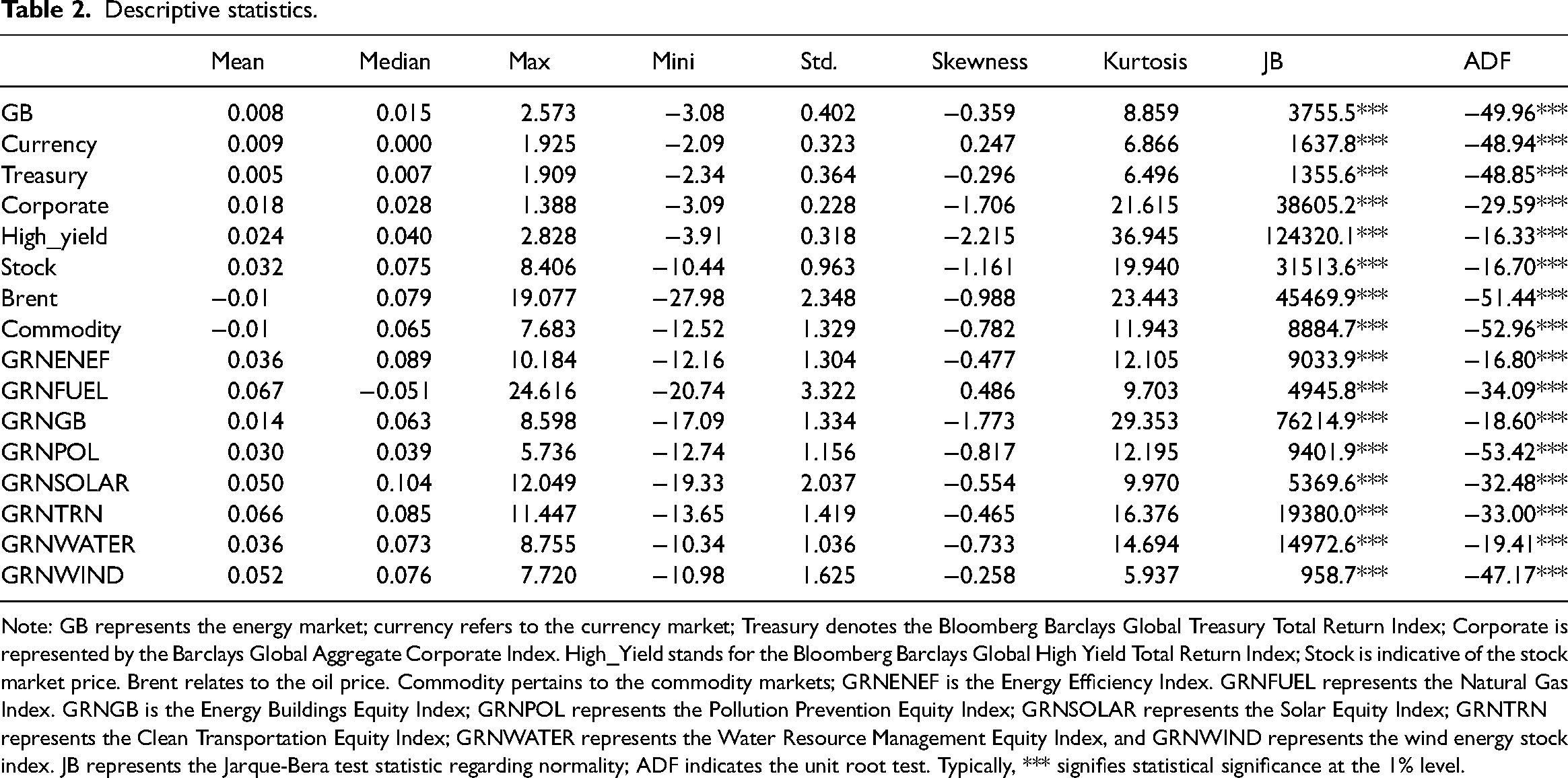
Note: GB represents the energy market; currency refers to the currency market; Treasury denotes the Bloomberg Barclays Global Treasury Total Return Index; Corporate is represented by the Barclays Global Aggregate Corporate Index. High_Yield stands for the Bloomberg Barclays Global High Yield Total Return Index; Stock is indicative of the stock market price. Brent relates to the oil price. Commodity pertains to the commodity markets; GRNENEF is the Energy Efficiency Index. GRNFUEL represents the Natural Gas Index. GRNGB is the Energy Buildings Equity Index; GRNPOL represents the Pollution Prevention Equity Index; GRNSOLAR represents the Solar Equity Index; GRNTRN represents the Clean Transportation Equity Index; GRNWATER represents the Water Resource Management Equity Index, and GRNWIND represents the wind energy stock index. JB represents the Jarque-Bera test statistic regarding normality; ADF indicates the unit root test. Typically, *** signifies statistical significance at the 1% level.

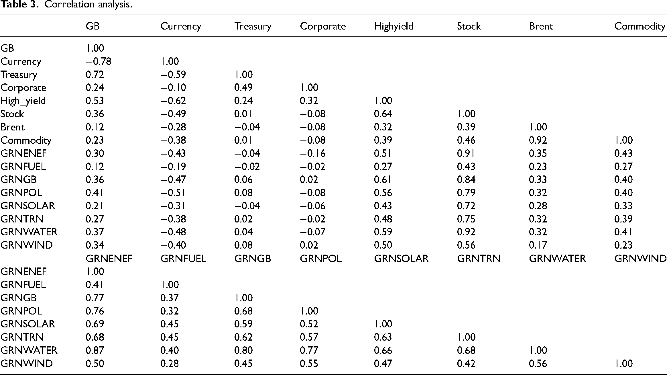
Table 3 presents the Pearson correlation coefficients for each asset pair across the entire sample period. Notably, a strong positive correlation (0.72) exists between the energy market and traditional treasury bonds, underscoring a significant relationship between the energy market and high-credit traditional bonds. The degree of Pearson correlation between energy markets and energy industry stocks appears both modest and varied, with correlations ranging from 0.12 in the Natural Gas sub-sector to 0.41 in the Pollution Prevention sub-sector. Such low correlations imply that, generally, the energy market and energy stocks might be influenced by distinct factors. Indeed, the correlations between the indices of energy stock sectors and traditional stock markets are generally more marked than those observed in energy market indices, with correlations exceeding 0.5 for all sectors except the natural gas sector. Additionally, the energy market's correlation with crude oil prices is notably low, at 0.12. Energy stocks also display modest positive correlations with crude oil, with values between 0.17 and 0.32. It's important to highlight that energy equities correlate weakly with traditional bond assets, including Treasury and corporate bonds.

Table 3.

Correlation analysis.

	GB	Currency	Treasury	Corporate	Highyield	Stock	Brent	Commodity
GB	1.00
Currency	−0.78	1.00
Treasury	0.72	−0.59	1.00
Corporate	0.24	−0.10	0.49	1.00
High_yield	0.53	−0.62	0.24	0.32	1.00
Stock	0.36	−0.49	0.01	−0.08	0.64	1.00
Brent	0.12	−0.28	−0.04	−0.08	0.32	0.39	1.00
Commodity	0.23	−0.38	0.01	−0.08	0.39	0.46	0.92	1.00
GRNENEF	0.30	−0.43	−0.04	−0.16	0.51	0.91	0.35	0.43
GRNFUEL	0.12	−0.19	−0.02	−0.02	0.27	0.43	0.23	0.27
GRNGB	0.36	−0.47	0.06	0.02	0.61	0.84	0.33	0.40
GRNPOL	0.41	−0.51	0.08	−0.08	0.56	0.79	0.32	0.40
GRNSOLAR	0.21	−0.31	−0.04	−0.06	0.43	0.72	0.28	0.33
GRNTRN	0.27	−0.38	0.02	−0.02	0.48	0.75	0.32	0.39
GRNWATER	0.37	−0.48	0.04	−0.07	0.59	0.92	0.32	0.41
GRNWIND	0.34	−0.40	0.08	0.02	0.50	0.56	0.17	0.23
	GRNENEF	GRNFUEL	GRNGB	GRNPOL	GRNSOLAR	GRNTRN	GRNWATER	GRNWIND
GRNENEF	1.00
GRNFUEL	0.41	1.00
GRNGB	0.77	0.37	1.00
GRNPOL	0.76	0.32	0.68	1.00
GRNSOLAR	0.69	0.45	0.59	0.52	1.00
GRNTRN	0.68	0.45	0.62	0.57	0.63	1.00
GRNWATER	0.87	0.40	0.80	0.77	0.66	0.68	1.00
GRNWIND	0.50	0.28	0.45	0.55	0.47	0.42	0.56	1.00

Dependence analysis using time-varying Copula models

Estimation of time-varying Copula-GARCH models

This section delves into the estimation of dynamic dependence and time-varying tail correlations between the energy market and other associated assets. The methodology involves: (a) Estimating all parameters in the marginal distribution functions of the variables using the AR(1)-GARCH(1, 1)-SkT model. (b) Gauging both static and dynamic dependencies between the energy market and related assets. This is done by estimating diverse static and dynamic Copula model parameters to elucidate these relationships. (c) Estimating the dynamic tail dependence between the energy market and the associated markets. The descriptive statistics reveal that all the time series exhibit pronounced tails and peaks. None adhere to a normal distribution, and they all display characteristics of smoothness and the ARCH effect. Consequently, this study adopts the AR(1)-GARCH(1,1)-SkT model to capture the marginal distributions for each market. Estimation results are delineated in Table 4.

Table 4.

Marginal distribution model estimation results.

	GB	Currency	Treasury	Corporate	High-yield	Stock	Commodity	Brent
0	0.008 (1.45)	0.012** (2.24)	0.006 (0.90)	0.022*** (5.70)	0.020*** (5.47)	0.051*** (4.20)	−0.005 (−0.23)	−0.001 (−0.02)
1	0.007 (0.53)	0.028 (1.46)	0.038* (1.98)	−0.017 (−0.76)	0.319*** (15.55)	0.079*** (4.12)	−0.030 (−1.62)	−0.062*** (−3.18)
ω	0.001** (2.50)	0.001*** (2.94)	0.002** (2.22)	0.002** (2.92)	0.002*** (4.05)	0.016*** (3.86)	0.016*** (2.99)	0.046*** (3.19)
	0.046*** (5.46)	0.046*** (5.98)	0.051*** (4.49)	0.060*** (4.69)	0.174*** (6.79)	0.154*** (7.16)	0.066*** (6.88)	0.087*** (6.34)
	0.948*** (109.5)	0.948*** (119.16)	0.932*** (61.76)	0.899*** (38.68)	0.805*** (31.19)	0.833*** (39.95)	0.924*** (86.32)	0.909 (66.76)
υ	7.306*** (7.48)	6.867*** (7.53)	6.972*** (8.09)	10.160*** (5.51)	4.647*** (11.71)	6.256*** (8.77)	5.758*** (8.89)	4.805*** (10.31)
λ	−0.050 (−1.34)	0.064** (2.19)	−0.022 (−0.88)	−0.117*** (−4.23)	−0.101*** (−3.47)	−0.138*** (−5.24)	−0.139*** (−5.66)	−0.113*** (−4.49)
Diagnostic test
Log-likelihood	−857.076	−492.122	−834.023	486.821	447.617	−2813.16	−3990.7	−5182.84
Q(5)	5.531 [0.07]	3.256 [0.37]	3.238 [0.38]	13.075 [0.00]	19.319 [0.00]	2.846 [0.47]	6.345 [0.03]	4.530 [0.15]
Q(5)2	9.602 [0.01]	1.870 [0.64]	2.939 [0.41]	82.200 [0.00]	2.876 [0.43]	3.122 [0.38]	4.685 [0.18]	6.778 [0.06]
ARCH(5)	12.750 [0.00]	2.864 [0.31]	2.606 [0.35]	20.320 [0.00]	2.940 [0.29]	4.248 [0.15]	0.657 [0.84]	0.134 [0.98]

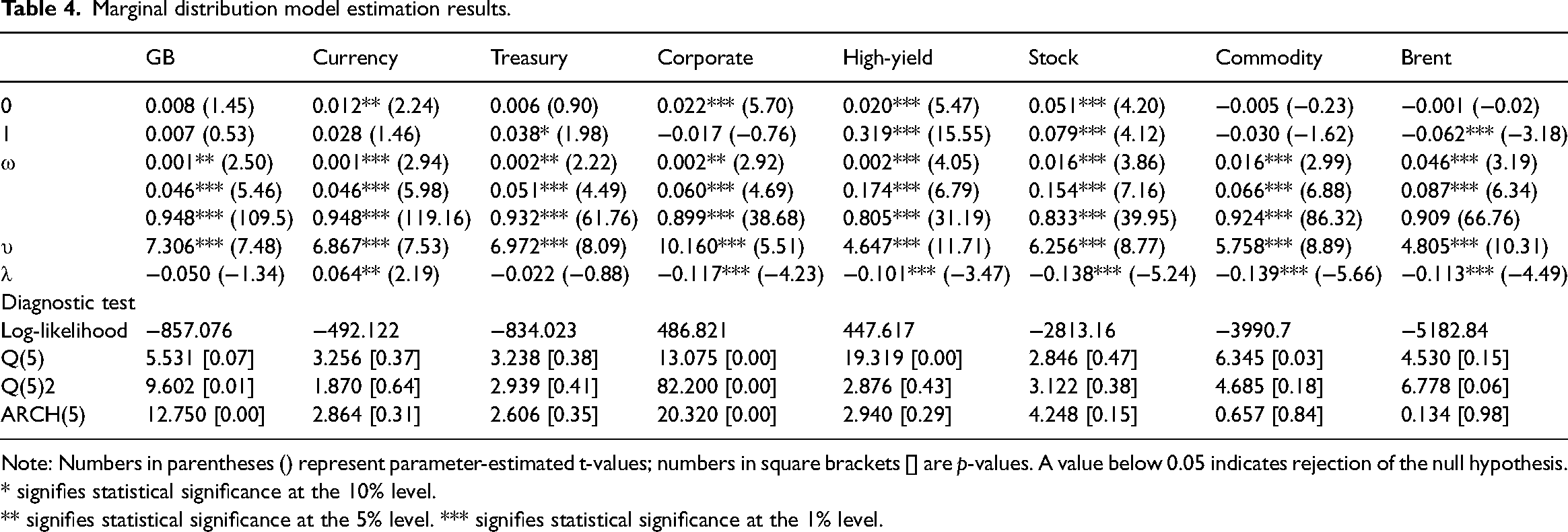
Note: Numbers in parentheses () represent parameter-estimated t-values; numbers in square brackets [] are p-values. A value below 0.05 indicates rejection of the null hypothesis.

* signifies statistical significance at the 10% level.

** signifies statistical significance at the 5% level. *** signifies statistical significance at the 1% level.

The results from Table 4 indicate that the coefficients of the mean equations, based on the ARMA model, are statistically significant. The GARCH model's effect on volatility is statistically significant for most of the time series. Furthermore, the sum of the estimated parameters “a” and “b,” which indicates the continuity of price rise volatility, approaches 1, thus satisfying the condition α1 + β1 < 1 . This suggests a pronounced volatility clustering effect across asset return indices. Additionally, for most datasets as denoted by lambda, there exists a substantial leverage effect. This implies that negative return shocks induce greater uncertainty than positive return shocks of the same magnitude.

Copula model selection

Upon determining the marginal distribution, we chose appropriate Copula functions to analyze the dependence structure between the two markets. Different Copula function models can yield varying results when interpreting this dependence structure. Generally, the AIC serves as the primary criterion for Copula function selection. In this research, we considered seven prevalent Copula models: Student-t, Clayton, Gumbel, Rotated Gumbel, SJC, Gaussian, and BB7. These models were applied to the marginal distribution for correlation fitting. The best-fitting Copula model was then chosen based on the lowest AIC value. The fitting efficacy of each Copula model, as depicted by their AIC values, can be found in Table 5.

Table 5.

AIC values for selected common Copula models.

	Student	Clayton	Gumbel	Rotated Gumbel	SJC	Gaussian	BB7
Currency	-2288.5	2.4	2.8	2.8	134.8	-2179.3	9.2
Treasury	-2715.1	-2054.0	-2469.3	-2522.0	-2545.7	-2473.0	-2534.0
Corporate	-323.1	-258.3	-234.9	-297.0	-292.4	-238.8	-309.0
High-yield	-1245.0	-891.6	-1125.7	-1113.6	-1168.2	-1075.9	-1185.5
Stock	-280.9	-168.0	-244.8	-216.5	-236.6	-217.5	-245.3
Commodity	-102.5	-103.1	-66.4	-111.9	-108.1	-86.5	-107.1
Brent	-46.3	-58.3	-20.5	-60.1	-56.3	-39.7	-59.1
GRNENEF	-140.7	-77.4	-121.8	-99.5	-119.3	-96.6	-135.7
GRNFUEL	-27.2	-30.3	-11.7	-31.7	-25.8	-23.6	-28.4
GRNGB	-238.0	-163.3	-200.8	-197.3	-218.5	-191.7	-233.3
GRNPOL	-350.6	-243.6	-307.9	-297.4	-329.6	-299.0	-346.2
GRNSOLAR	-52.3	-31.9	-24.7	-39.6	-38.2	-27.2	-37.8
GRNTRN	-139.2	-100.1	-110.3	-117.2	-132.1	-114.6	-132.6
GRNWATER	-249.1	-179.5	-224.6	-223.0	-244.0	-220.3	-253.3
GRNWIND	-278.0	-195.0	-217.2	-239.4	-250.7	-219.4	-251.2

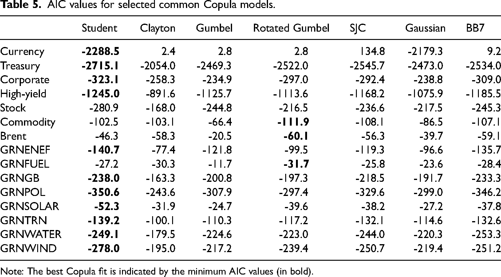
Note: The best Copula fit is indicated by the minimum AIC values (in bold).

According to the AIC, the optimal fit between the returns of the energy market and the majority of traditional assets is the Time-Varying Student-t Copula model. This indicates a symmetric dependence between the energy market and most of the traditional financial and energy markets. Such a dependence model suggests that both negative and positive international market return news similarly affect the energy market. However, the optimal Copula model describing the relationship between the energy markets is the Rotated Gumbel. This model captures the asymmetric tail dependence, indicating that negative news in one energy market profoundly influences the other more than positive news does.

From the Copula model selection outlined above, this study adopts the dynamic Rotated Gumbel model to describe the interdependence and structure between two distinct energy markets. Conversely, the dynamic Student-t Copula model is employed to delineate the interdependence and structure between the energy market and other financial markets.

Correlation analysis using static and time-varying Copula models

This study computes dynamic dependence through a 180-degree rotated Gumbel Copula model. The dynamic relationship between the energy market and the commodity, oil, and energy fuel markets manifest as positive and irregular, fluctuating around the value of 1. Such findings suggest that surges in crude oil and commodity prices escalate production expenses. These increased costs subsequently stimulate sectors like renewable energy, augmenting the demand for energy investment capital. This amplification operates via three channels: the substitution effect, the aggregate demand effect, and the production disincentive effect.

For the remaining correlated assets, the dynamic correlation coefficients largely mirror a similar trajectory. A notable rise in interdependence transpired during the Russia-Ukraine conflict in 2022. However, this heightened correlation receded from May 2022, only to surge again during the stock market downturn in June 2022. After this resurgence, a fluctuating decline was observed. The study further underscores that dynamic interdependence isn't perpetually positive, being contingent largely on external economic climates. Specific peaks in interdependence between energy and financial markets materialize at distinct junctures, primarily due to significant disruptive events. Financial crises, oil-centric conflicts, and shifts in socio-political landscapes can recalibrate market supply and demand dynamics, intensifying price volatility. This, in turn, amplifies risk contagion and market interdependence.

To summarize, the empirical scrutiny in this segment divulges two salient observations: (a) Except for money markets, energy markets and related assets exhibit a predominant positive time-varying dependence in return realizations. (b) A symmetric tail dependence exists between energy markets and a majority of financial and energy markets. In contrast, there's an asymmetric tail dependence on the commodities, oil, and energy fuel markets. This indicates that unfavorable outcomes in the energy market exert a more pronounced influence than positive ones. Such dependencies are considerably swayed by investor sentiment, thereby endorsing the “asymmetric price adjustment” theory between equity and debt markets. Moreover, considering the informational interplay across these markets and their historical volatility, it's inferred that the bond between energy markets and their allied assets intensifies during economic upheavals.

Test for structural breakpoints in dynamic dependence

A “structural mutation” refers to a shift in the trajectory of a series at a point when variables that mirror its attributes undergo significant changes, such as the Russian-Ukrainian conflict, financial crises, currency upheavals, oil disruptions, or wars. Emerging markets frequently exhibit susceptibility to these structural alterations, often stemming from the adoption of pertinent economic policies, modifications in financial regulatory frameworks, or the repercussions of abrupt, significant economic or political crises, both domestically and internationally. Such disruptions can precipitate pronounced shifts in the interconnectedness of different markets. Therefore, a meticulous analysis of abrupt structural alterations can shed light on the intricate, evolving interrelationships between energy markets and other sectors, illustrating the multifaceted interdependence between energy markets and their associated assets.

In this study, we employ Bai and Perron's test for structural breakpoints to ascertain the exact positions of these shifts in the interconnectedness between energy markets and related assets. For this test, the correction value is fixed at 0.1, the maximum count of breakpoints is set to 7, and the significance level is maintained at 5%. This approach aids in detecting the number and precise dates of structural breakpoints across all correlated assets. The findings of this test are detailed in Table 6. As deduced from Table 6, there exist a minimum of five structural breakpoints in the trajectory of evolving dependencies between energy markets and linked assets. In this study, we synchronize the timing of these structural shifts with real-world events. Notably, we focus on events within the sample period to pinpoint the locations of these breakpoints. Alongside this, we identify major crisis incidents within the sample as primary triggers inducing shifts in market dependence.

Table 6.

Statistics of structural breakpoints.

Variant	Statistics of structural mutation points
	SupFT (1/0)	SupFT (2/1)	SupFT (3/2)	SupFT (4/3)	SupFT (5/4)
Currency	1873.6	816.0861	87.34194	113.965	407.5502
Treasury	3230.311	224.9881	47.5985	82.71615	53.14662
Corporate	5751.276	849.4069	238.7711	389.9201	335.3738
High-yield	1098.143	276.1513	733.3513	402.5171	369.6571
Stock	3800.686	247.5895	141.7422	244.7391	279.71
Commodity	5828.197	183.384	129.3104	66.25177	192.8101
Brent	3980.272	76.44158	77.30107	144.2307	35.01218
GRNENEF	4033.319	212.213	105.1795	86.18598	120.4982
GRNFUEL	153.7259	162.5955	56.35914	113.7741	48.44907
GRNGB	2397.581	184.8271	425.205	150.3049	136.7507
GRNPOL	2471.419	195.6997	241.0274	448.7617	248.2813
GRNSOLAR	6390.477	152.9532	133.5015	131.6775	295.6442
GRNTRN	3974.378	254.9318	141.291	302.0782	132.3307
GRNWATER	2723.864	99.99041	246.5343	182.7947	83.77416
GRNWIND	2112.023	1068.522	822.6115	220.0206	244.3021

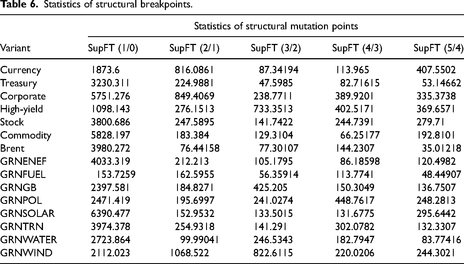
In summary, the energy market experienced several structural breakpoints correlating with significant global events: (a) 11 May 2014: Russian forces occupied Rimia and parts of the Donetsk and Luhansk regions. (b) 22 February 2015: The defense of Donetsk airport concluded after 242 days. While the Minsk II agreement was formalized, Ukrainian forces were compelled to withdraw from Debaltseve. (c) 5 February 2017: A marked military escalation transpired in Avdeevka accompanied by extensive cyberattacks on Ukrainian entities. (d) 2 May 2018: The law on Donbas reintegration was ratified, heralding the commencement of the Joint Forces’ operation, notably post the Kerch Strait incident. (e) 12 March 2020: The World Health Organization (WHO) delineated the escalating cases of novel coronavirus pneumonia as the onset of the COVID-19 global pandemic. On 11 March, WHO's Director-General reported a global case count exceeding 118,000, with 4291 fatalities. Owing to the escalating nature of the epidemic and subpar response in certain territories, it was officially classified as a “global pandemic.” Following this proclamation, the pandemic perpetuated its global spread, reaching alarming rates of transmission. (f) 15 April 2021: Russia obstructed a section of the Black Sea and amassed approximately 120,000 troops along the Ukraine border. (g) 24 February 2022: Russia initiated a comprehensive invasion of Ukraine. These episodes underscore the profound influence of substantial crises—ranging from financial downturns and oil-centered conflicts to shifts in economic and political landscapes—on market dynamics. Such pivotal events can markedly sway supply-demand equilibriums and induce pronounced price fluctuations, thereby magnifying risk contagion and inter-market correlations.

Conclusion

In our study, we analyzed the energy market index with 15 related asset returns, including both traditional financial assets and energy industry stock markets. Using GARCH-Copula models and the BP test method, we captured the dependence between the energy market and associated assets, identifying mutation points related to the Russia-Ukraine conflict.

Employing the AR(1)-GARCH(1,1)-SkT model, our results showed significant coefficients in the ARMA-based mean equation. The GARCH parameters demonstrated volatility clustering, and we noted a stronger uncertainty impact from negative versus positive return shocks.