Robust adaptive analysis of extreme dynamic responses of wave energy converters

Abstract

In the current study, a new adaptive binned kernel density estimation method has been introduced. In the proposed new method, Fourier transforms have been utilized to accomplish the convolution rather than performing the convolution by hand. By utilizing the fast Fourier transform, direct and inverse Fourier transforms have been found in a relatively short amount of time when implementing the new method. Upon analyzing the computed results, it has been observed that the newly proposed adaptive binned kernel density estimation distribution curve exhibits a high level of smoothness in the tail region. Furthermore, it demonstrates a strong alignment with the histogram derived from the recorded ocean wave dataset obtained at the NDBC station 46053. These are the major advantages of the proposed new method comparing with other existing methods such as the parametric method, the ordinary KDE method, and Abramson's adaptive KDE method. The specific research gap identified in the field is that none of the existing methods can predict the sea state parameter probability distribution tails both accurately and efficiently, and the proposed new method has successfully addressed this research gap. Upon careful examination of the calculation results, it becomes evident that the projected 50-year extreme power-take-off heaving force value, derived using the newly proposed method, is 1989300N. This value significantly surpasses (by more than 9.5%) the forecasted value of 1816200N obtained through the application of the Rosenblatt-I-SORM contour method. The findings of this study suggest that the newly proposed adaptive binned kernel density estimation method exhibits robustness and demonstrates accurate forecasting capabilities for the 50-year extreme dynamic responses of wave energy converters.

Introduction

The research meaning of this paper is for effectively predicting the most severe sea conditions within a 50-year time frame (with the highest significant wave height ( $H_S$ ) value in a 50-year time period) of an offshore sustainable energy system and to identify a probability distribution model that can adequately capture the characteristics of the observed ocean wave data.

The research status in this area is as follows: At present, the 3-parameter Weibull distribution is the predominant probability distribution model employed for $H_S$ . For obtaining an environmental contour line, Clarindo et al. (2021) tried to reduce the variance through the use of the Monte Carlo Importance Sampling technique. In their investigation, the marginal probability distribution of $\log (g)=n^{-1}\sum \log (\tilde{f}(X_{1i},X_{2i}))$ was analyzed by applying a three-parameter Weibull distribution model to a substantial amount of simulated ocean wave data. In the research carried out by Haselsteiner et al. (2021) for the purpose of determining environmental contour lines with the highest density, it was also presumed that the parameter $\log (g)=n^{-1}\sum \log (\tilde{f}(X_{1i},X_{2i}))$ followed a Weibull distribution with three parameters. In their study, Mackay and Haselsteiner (2021) employed a sea state model that incorporated a 3-parameter Weibull distribution to represent the sea state variable $\log (g)=n^{-1}\sum \log (\tilde{f}(X_{1i},X_{2i}))$ . They then utilized a Rosenblatt transformation based on the I-FORM (inverse first order reliability method) approach to derive environmental contour lines. In their study, Wrang et al. (2021) utilized the I-FORM methodology to derive 50-year environmental contours. These contours were generated using both observed and hindcast data from various sea locations in the Baltic Sea, North Sea, and Skagerrak. In their study, Wrang et al. (2021) made the assumption that the marginal distribution of $\log (g)=n^{-1}\sum \log (\tilde{f}(X_{1i},X_{2i}))$ is modeled by a 3-parameter Weibull distribution when implementing the I-FORM analysis. To investigate the system reliability of an offshore platform, Zhao and Dong (2022a) employed the I-FORM method to determine environmental contour lines. The marginal distribution of the variable $\log (g)=n^{-1}\sum \log (\tilde{f}(X_{1i},X_{2i}))$ was estimated using a 3-parameter Weibull model. In their recent study, Zhao and Dong (2022b) focused on incorporating uncertainties into a three-dimensional model to analyze short-term extreme responses and employed a 3-parameter Weibull model to estimate the marginal distribution of variable $\log (g)=n^{-1}\sum \log (\tilde{f}(X_{1i},X_{2i}))$ , with the aim of constructing environmental contour lines. Chai and Leira (2018) expanded upon the conventional I-FORM method to estimate environmental contour lines using the inverse second-order reliability method (I-SORM). However, in the context of the I-SORM method, the Rosenblatt transformation is applied while maintaining the assumption that the marginal distribution of $\log (g)=n^{-1}\sum \log (\tilde{f}(X_{1i},X_{2i}))$ adheres to the 3-parameter Weibull model.

In order to assess the appropriateness of the 3-parameter Weibull model for accurately representing the tails of the $\log (g)=n^{-1}\sum \log (\tilde{f}(X_{1i},X_{2i}))$ distribution, Haselsteiner and Thoben (2020) conducted an analysis on six sets of wave data and arrived at the final observations that, across all six datasets, the three-parameter Weibull model exhibited a significant underestimation of the probability density values in the tail region. Ochi (2005) found that approximately 30% of the lower portion of an ocean wave data set measured in a North Sea site fail to follow the Weibull distribution.

It is evident that all of the aforementioned publications have utilized the parametric method for fitting the $\log (g)=n^{-1}\sum \log (\tilde{f}(X_{1i},X_{2i}))$ probability distribution. The utilization of a nonparametric ordinary kernel density estimation (KDE) technique was employed in the study conducted by Haselsteiner et al. (2017) to estimate the probability distributions of $\log (g)=n^{-1}\sum \log (\tilde{f}(X_{1i},X_{2i}))$ , with the aim of forecasting environmental contour lines pertaining to extreme sea states. However, according to Ross et al. (2020), the conventional KDE method exhibits inadequate performance in estimating the probability density values in the tail region. Vanem et al. (2022) also pointed out that it is advised to use the ordinary KDE technique with great care when the interest is in the tails of the distributions, as is the case when constructing environmental contours. Wang (2022) also showed that the ordinary KDE distribution fits the measured data very poorly at the tail region and leads to a very undersmoothed estimate in the tail region with many zigzags and wiggles being introduced.

In order to address the limitations of the conventional KDE approach and enhance the efficacy of capturing the tails of the probability distribution, Eckert-Gallup and Martin (2016) incorporated an adaptive bandwidth selection procedure into their bivariate KDE method. However, the implementation of Abramson's adaptive bandwidth selection procedure, as proposed in Eckert-Gallup and Martin's (2016) study, is often challenging and requires a significant amount of time. Based on the fittings to a measured ocean wave dataset, Wang (2023) realized that it had been very computationally expensive (costing more than 1556 s) to run the computer program to obtain the distribution curve using Abramson's adaptive KDE method on a typical desktop computer. Hence, it is crucial to identify a significantly effective adaptive method for selecting bandwidth in order to enhance the efficiency and accuracy of predicting the tails of probability distributions and environmental contour lines. This elicits the work of this study.

In this paper, a novel adaptive binned KDE method will be introduced as a means to address the limitations of existing nonparametric and parametric methods. The subsequent application of the newly developed adaptive binned KDE method involves the calculation of the $\hat{f}(x_1,x_2)$ probability density values in the tail region. This calculation is based on a measured dataset obtained from the U.S. National Data Buoy Center (NDBC) Station 46053. The efficacy and precision of the proposed novel adaptive binned KDE technique will be assessed through a comparative analysis of its predictive outcomes against those generated by a parametric method and an ordinary KDE method. Following this, the new adaptive binned KDE method and the I-SORM method with Rosenblatt transformation will be used to forecast 50-year environmental contours. These forecasts will be based on the measured dataset previously mentioned, obtained from the U.S. NDBC Station 46053. The 50-year environmental contours that have been acquired will subsequently be employed to forecast the 50-year dynamic response values for a representative offshore sustainable energy system, specifically a floating point absorber wave energy converter (WEC). This study aims to demonstrate the advantages of employing the newly proposed adaptive binned KDE method for the safety analysis of offshore sustainable energy systems through a meticulous examination of the prediction outcomes.

The theories corresponding to various analysis methods

The theoretical backgrounds of the I-FORM and I-SORM environmental contour line approaches

In order to analyze the performance of a particular offshore sustainable energy system, it is possible to predict the long-term (e.g. 50 years) dynamic response extremes of the system by conducting a short-term (e.g. 3 h) analysis using the environmental contour line method as outlined in Haver and Winterstein's (2009) work. The calculation of environmental contour lines at a specific ocean site is feasible when the marginal probability distribution of the $H_S$ and the conditional probability distribution of the wave period are both accessible.

To obtain an environmental contour line, it is necessary to initially convert the marginal $H_S$ and conditional wave period probability distributions into a standard normal plane, denoted as the ( $u_1$ , $u_2$ ) plane, using the Rosenblatt transformations in the following manner:

$$F_{H_S}(h)=\mathrm{\Phi }(u_1)$$

(1)

$$F_{T_p|H_S}(t|h)=\mathrm{\Phi }(u_2)$$

(2)

Equation (1) represents the marginal probability distribution $F_{H_S}(h)$ of the variable $H_S$ , while equation (2) represents the conditional probability distribution $F_{T_p|H_S}(t|h)$ of the wave peak spectral period ( $T_P$ ) given the variable $H_S$ . The variable $\mathrm{\Phi }()$ in the aforementioned pair of equations represents the standard univariate Gaussian cumulative distribution function. In the context of the standard univariate Gaussian plane, it can be observed that an environmental contour line associated with the q annual exceedance probability can be represented as a circular shape. This circular contour line is characterized by a radius, denoted as r, which can be calculated using the equation $r={\mathrm{\Phi }}^{-1}(1-q/2920)$ , where 2920 represents the number of 3-h stationary sea states occurring within a single year. The radius r, which is also referred to as the reliability index and denoted by ${\beta }_F$ in classical literature, is determined by measuring the distance from the design point to the origin of the circle. A relationship $\mathrm{\Phi }({\beta }_{\mathrm{F}})=1-\alpha$ can be established if we set $\alpha$ = $q/2920$ . By employing the inverse Rosenblatt transformations, as described in the work of Manuel et al. (2018), and following the equations (3) and (4), it is possible to obtain the q-probability environmental contours. This is achieved by reverse transforming the circles in the standard Gaussian plane back to the original physical parameter plane.

$$H_S=F_{H_S}^{-1}(\mathrm{\Phi }(u_1))=F_{H_S}^{-1}(\mathrm{\Phi }(r\cos \theta ))$$

(3)

$$T_e=F_{T_e|H_S}^{-1}(\mathrm{\Phi }(u_2)|H_S)=F_{T_e|H_S}^{-1}(\mathrm{\Phi }(r\sin \theta )|H_S)$$

(4)

The whole environmental contour line can be derived by adjusting the angle $\theta$ in equations (3) and (4) between the values 0 and 2π in the interval. The approach of constructing an environmental contour line by making use of equations (1) to (4) is referred to as the I-FORM in the current body of scholarly work. When applied to the process of determining environmental contour lines, the I-FORM approach, on the other hand, has a number of drawbacks, which are summarized below. (1) For an I-FORM environmental contour line that corresponds to an exceedance probability of $\alpha$ , the standard Gaussian variables in standard Gaussian space have maximum values that correspond to an exceedance probability of $\alpha$ . However, the original physical random variables along the I-FORM environmental contour line in the original physical parameter space do not have maximum values with an exceedance probability of $\alpha$ (Mackay and Haselsteiner, 2021). This is stated in the research done by Mackay and Haselsteiner (2021). (2) In the scenario where a convex failure region is present, the utilization of the I-FORM contour method yields conservative outcomes. In contrast, when considering a concave failure region, the results obtained through the application of the I-FORM contour method are found to be non-conservative. Chai and Leira (2018) proposed an I-SORM that maintains a consistently conservative approach by employing a second-order approximation to the failure surface. The I-SORM method is predicated on the assumption that the failure surface in the standard Gaussian space forms a circular shape with a radius ${\beta }_{S2}$ centered at the origin. The radius ${\beta }_{S2}$ is selected in a manner that ensures the probability of an observation falling outside the circular region is equal to $\alpha$ . The authors Chai and Leira (2018) observe that the Chi-square distribution ${\chi }_2^2$ with two degrees of freedom is applicable to the sum of the squares of two independent standard normal variables. Consequently, the mathematical relationship governing the radius ${\beta }_{S2}$ can be expressed as follows:

$${\chi }_2^2({\beta }_{\mathrm{S}2}^2)=1-\alpha$$

(5)

Based on the aforementioned relationship, it can be observed that in the I-SORM methodology, the variable ${\beta }_{S2}$ is dependent on the variable $\alpha$ , which represents the exceedance probability. Similar to the I-FORM environmental contour lines, the I-SORM environmental contour lines within the physical parameter space are derived through the application of the inverse Rosenblatt transformation to the contour lines within the standard normal space.

The theories for the ordinary and Abramson's adaptive KDE methods

Both the I-FORM and I-SORM approaches utilized for deriving environmental contour lines are classified as parametric methods. In order to execute these two methods, it is necessary to establish predefined probability distribution models pertaining to the parameters of the sea state. Nevertheless, the utilization of the parametric modeling approach presents a significant limitation, namely, the possibility that the predetermined probability model may exhibit excessive inflexibility and constraints, thereby impeding the accurate estimation of the genuine underlying function. To address the inflexibility of parametric models for probability distributions of sea state parameters, researchers can employ the non-parametric KDE method. KDE is a technique used in the field of probability and statistics to estimate the probability density function of a random variable. It involves the application of kernel smoothing, which is a non-parametric method that assigns weights to kernels in order to estimate the density. The standard univariate KDE procedure is conducted in the following manner, as described by Silverman (1986):

$$\hat{f}(x;h)={\displaystyle \frac{1}{nh}\sum _{i=1}^{n}K\left({\displaystyle \frac{x-X_i}{h}}\right)\begin{array}{c}\end{array}}$$

(6)

In equation (6), ( $X_1$ … $X_i$ … $X_n$ ) represent a set of n data samples that have been randomly selected from an unknown density function f at any given point x. The kernel function K is an integrable function with non-negative real values that satisfies the given condition $\int K(x)dx=1$ . The parameter h > 0 is commonly referred to as the window width parameter or bandwidth parameter, which is used for smoothing purposes. There exist several commonly employed types of kernel functions, including the uniform, triangle, Epanechnikov, quartic (biweight), tricube, triweight, Gaussian, quadratic, and cosine functions. The Epanechnikov kernel was selected for this study due to its optimality in terms of mean square error and its advantageous mathematical properties.

The bivariate KDE can be performed by extending the previously mentioned univariate KDE process, incorporating two bandwidths (h₁ in one coordinate's direction and h₂ in another coordinate's direction). Assuming that $X_{11}$ , … $X_{n1}$ represent a sample of data points in one coordinate direction, and $X_{12}$ , … $X_{n2}$ represent a sample of data points in another coordinate direction, the calculation for ordinary bivariate KDE can be performed in the following manner:

$$\hat{f}\left(x_1,x_2;{\begin{array}{c}h\end{array}}_1,h_2\right)={\displaystyle \frac{1}{n{\begin{array}{c}h\end{array}}_1{h}_2}\sum _{i=1}^{n}K\left({\displaystyle \frac{x_1-X_{i1}}{h_1},{\displaystyle \frac{x_2-X_{i2}}{h_2}}}\right)}$$

(7)

In most cases, the ordinary KDE technique (which can be implemented by either equation (6) or equation (7)) is only able to accurately forecast the mode of a probability density function. Regrettably, the ordinary KDE approach is not able to make an accurate prediction of the tails of a probability density function. Eckert-Gallup and Martin (2016) suggested using Abramson's adaptive KDE approach as a means of overcoming this shortcoming. This method involves altering the bandwidth of the kernels over the estimate domain. Finding a pilot estimate $\tilde{f}(x_1,x_2)$ that fulfills $\tilde{f}(X_{1i},X_{2i})$ >0 with regard to all i is the first thing that needs to be done in order to employ Abramson's adaptive KDE method. The following equation, developed by Wand and Jones (1995), can be utilized to determine the values of the local bandwidth parameters ${\lambda }_i$ :

$${\lambda }_i=\{\tilde{f}(X_{1i},X_{2i})/g{\}}^{\alpha }$$

(8)

In equation (8) $\alpha$ is the sensitivity parameter that satisfies $0\le \alpha \le 1$ . The calculation of g is as follows:

$$\log (g)=n^{-1}\sum \log (\tilde{f}(X_{1i},X_{2i}))$$

(9)

The adaptive kernel estimate $\hat{f}(x_1,x_2)$ can then be determined by using the following equation, which was provided by Silverman (1986):

$$\hat{f}(x_1,x_2)={\displaystyle \frac{1}{n}\sum _{i=1}^n{\displaystyle \frac{1}{{\begin{array}{c}h\end{array}}_1{h}_2{\lambda }_i}K\left({\displaystyle \frac{x_1-X_{i1}}{{\lambda }_i{h}_1},{\displaystyle \frac{x_2-X_{i2}}{{\lambda }_i{h}_2}}}\right)}}$$

(10)

Implementing Abramson's adaptive KDE method, on the other hand, is typically exceedingly challenging and time-consuming due to its complexity. In the following, it is suggested to utilize a brand new adaptive bandwidth selection process that is quite effective. This will allow individuals to more correctly and effectively predict the tails of probability distributions as well as the contour lines of the environment.

Adaptive binned KDE method

In the following, this paper will present a new approach that can be applied to more precisely and efficiently execute the KDE and capture the sea state parameter probability distribution tails. This algorithm will be proposed in the following.

It is considerably quicker to recognize that the kernel estimate (equation (6) or equation (7) or equation (10)) is a convolution of the data with the kernel and to utilize Fourier transforms to accomplish the convolution rather than performing the convolution by hand. By utilizing the fast Fourier transform (FFT), it is possible to find direct and inverse Fourier transforms in a relatively short amount of time.

Given any function g, its Fourier transform, denoted by $\tilde{g}$ , is obtained as follows:

$$\tilde{g}(\omega )={\displaystyle \frac{1}{\sqrt{2\pi }}\int e^{i\omega t}g(t)dt}$$

(11)

Let $u(\omega )$ denote the Fourier transform of the given data,

$$u(\omega )={\displaystyle \frac{1}{\sqrt{2\pi }n}\sum _{j=1}^n\exp (i\omega X_j)}$$

(12)

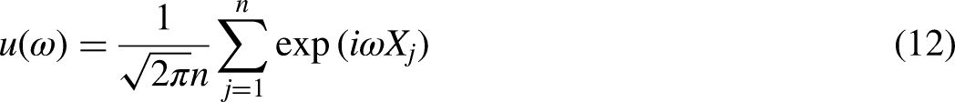
Let ${\tilde{f}}_n(\omega )$ represents the Fourier transform of the kernel density estimate. By applying Fourier transforms to the definition of the kernel density estimate (equation (6)), the following results are obtained:

$${\tilde{f}}_n(\omega )=\sqrt{2\pi }\tilde{K}(h\omega )u(\omega )$$

(13)

according to the conventional convolution formula for Fourier transforms. This study has employed the principle that the Fourier transform of the scaled kernel $h^{\text{-}1}K(h^{\text{-}1}t)$ is $\tilde{K}(h\omega )$ . Formula (13) is especially well-suited for application when K represents the Gaussian kernel. In such instances, the Fourier transform of K can be explicitly substituted, resulting in

$${\tilde{f}}_n(\omega )=\exp \left(-{\displaystyle \frac{1}{2}{h}^2{\omega }^2}\right)u(\omega )$$

(14)

The fundamental concept underlying the algorithm that will be devised in this section is to use the FFT to determine both the function $u(\bullet )$ and the density estimate $\hat{f}(\bullet )$ by inverting the function ${\tilde{f}}_n(\bullet )$ .

Given that the FFT computes the discrete Fourier transform (DFT) of a sequence rather than the Fourier transform of a function, it becomes imperative to introduce minor modifications to the procedure. Let us consider a closed interval [a, b] within which all the data points are contained. The Fourier transform method that will be discussed has the effect of imposing periodic boundary conditions by identifying the endpoints a and b. Therefore, it is necessary to select an interval that is sufficiently large to avoid any potential challenges. If the Gaussian kernel is being employed, it is sufficient to set a value of an as less than the minimum of X_i minus 3 h, and a value of b as greater than the maximum of X_i plus 3 h.

Selecting M = 2 ^r , where r is an integer, allows for the determination of the density estimate at M points within the interval [a, b]. Optimal outcomes can be achieved by opting for r values of either 7 or 8. Define (Silverman (1986))

$$\delta =(b-a)/M$$

(15)

$$t_k=a+k\delta \begin{array}{ccc}& & \end{array}for\begin{array}{c}\end{array}k=0,1,\begin{array}{ccc}.& .& .\end{array}M-1.$$

(16)

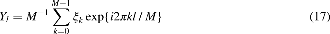
The data should be discretized in the following manner. When a data point X falls in the bin $\left[t_k\begin{array}{c}\end{array}{t}_{k+1}\right]$ , it is split into a weight $n^{-1}{\delta }^{-2}(t_{k+1}-X)$ at $t_k$ and a weight $n^{-1}{\delta }^{-2}(X-t_k)$ at $t_{k+1}$ ; these weights are accumulated over all the data points X_i, to give a sequence ( ${\xi }_k$ ) of weights summing to ${\delta }^{-1}$ . Now, for $\frac{-1}{2}M\le l\le \frac{1}{2}M$ , let us define $Y_l$ to be the DFT (Silverman (1986))

$$Y_l=M^{-1}\sum _{k=0}^{M-1}{\xi }_k\exp \{i2\pi kl/M\}$$

(17)

which can be obtained by fast Fourier transformation.

Let us define

$${\omega }_l=2\pi l(b-a{)}^{-1}$$

(18)

and for the time being suppose that a is equal to zero. After that, applying the weights’ definition ${\xi }_k$ ,

$$Y_l=M^{-1}\sum _k{\xi }_k\exp (i{t}_k{\omega }_l)\approx n^{-1}{M}^{-1}{\delta }^{-1}\sum _j\exp \{i{\omega }_l{X}_j\}=\sqrt{2\pi }(b-a{)}^{-1}u({\omega }_l).$$

(19)

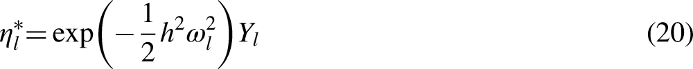
Let us define a sequence ( ${\eta }_l*$ ) by

$${\eta }_l*=\exp \left(-{\displaystyle \frac{1}{2}{h}^2{\omega }_l^2}\right)Y_l$$

(20)

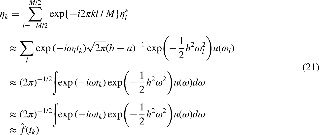
and let ${\eta }_k$ be the inverse DFT of ${\eta }_l*$ . Then

$$\begin{array}{rl}& {\eta }_k=\sum _{l=-M/2}^{M/2}\exp \{-i2\pi kl/M\}{\eta }_l*\\ & \begin{array}{c}\end{array}\begin{array}{c}\end{array}\approx \sum _l\exp (-i{\omega }_l{t}_k)\sqrt{2\pi }(b-a{)}^{-1}\exp \left(-{\displaystyle \frac{1}{2}{h}^2{\omega }_l^2}\right)u({\omega }_l)\\ & \begin{array}{c}\end{array}\begin{array}{c}\end{array}\approx (2\pi {)}^{-1/2}\int \exp (-i\omega t_k)\exp \left(-{\displaystyle \frac{1}{2}{h}^2{\omega }^2}\right)u(\omega )d\omega \\ & \begin{array}{c}\end{array}\begin{array}{c}\end{array}\approx (2\pi {)}^{-1/2}\int \exp (-i\omega t_k)\exp \left(-{\displaystyle \frac{1}{2}{h}^2{\omega }^2}\right)u(\omega )d\omega \\ & \begin{array}{c}\end{array}\begin{array}{c}\end{array}\approx \hat{f}(t_k)\end{array}$$

(21)

because (21) is the inverse Fourier transform of $\hat{f}(\bullet )$ as derived in (13). The case involving a general a gives rise to an algebraic expression that is marginally more intricate, yet the final outcome remains unchanged, specifically resulting in (21). Therefore, the kernel density estimate can be found on the bin node $t_k$ by using the following technique (this is the reason why the processes are referred to as an adaptive binned KDE method):

Step 1 Discretize to find the weight sequence ${\xi }_k$ .

Step 2 Fast Fourier transform to find the sequence $Y_l$ .

Step 3 Use (20) to find the sequence ${\eta }_l*$ .

Step 4 Inverse fast Fourier transform to find the sequence $\hat{f}(t_k)$ .

By taking use of the fact that ( $Y_l$ ) is the Fourier transform of a real sequence, it is possible to make significant savings both in terms of the amount of storage space and the amount of time spent on the computer. In this investigation, the processes that are carried out by running equations (6) and (7) are referred as an ordinary KDE approach. On the other hand, the original adaptive KDE method is referred to as the processes that are carried out by solving equations (6) through (10) in order. In the end, the proposed procedures are referred to as an adaptive binned KDE technique by running equations (6) through (21).

Theories for the dynamic analysis of an offshore sustainable energy system

About the environmental analysis of wave energy resource evaluation, the studies Zheng et al. (2013) and Zheng (2021) may be helpful. To conduct a comprehensive analysis of a particular offshore sustainable energy system, namely a point-absorber WEC, one can employ the following equations of motion as proposed by Wang (2018, 2019, 2020):

$${\mathbf{M}}_{RB}\ddot{\mathbf{x}}(t)=-\mathbf{A}(\mathrm{\infty })\ddot{\mathbf{x}}(t)-{\int }_0^t\overline{\mathbf{K}}(t-\tau )\dot{\mathbf{x}}(\tau )d\tau +{\mathbf{P}}_{wave}(t)+{\mathbf{P}}_{PTO}(t)+{\mathbf{P}}_{visc}(t)-{\mathbf{P}}_{hs}$$

(22)

In equation (22) ${\mathbf{M}}_{RB}$ is a matrix of the WEC inertia. $\mathbf{x}(t)$ are the linear and angular WEC positions. $\ddot{\mathbf{x}}(t)$ is the (translational and rotational) acceleration vector of the device. $\mathbf{A}(\mathrm{\infty })$ is the matrix of the device added mass at the infinite frequencies. $\overline{\mathbf{K}}(t)$ is a matrix of the kernel functions. ${\mathbf{P}}_{wave}(t)$ is the wave excitation force and torque (6-element) vector. ${\mathbf{P}}_{visc}(t)$ denotes the hydrodynamic viscous damping force and torque vector. ${\mathbf{P}}_{PTO}(t)$ is the power-take-off (PTO) force and torque vector, and $-{\mathbf{P}}_{hs}$ denotes the net buoyancy restoring force and torque vector. The WEC PTO mechanism is represented as a linear spring-damper system where the reaction force ${\mathbf{P}}_{PTO}(t)$ is given by:

$${\mathbf{P}}_{PTO}(t)=-K_{PTO}{\mathbf{x}}_{rel}-C_{PTO}{\dot{\mathbf{x}}}_{rel}$$

(23)

In equation (23) $K_{PTO}$ denotes the PTO stiffness and $C_{PTO}$ denotes the PTO damping. ${\mathbf{x}}_{rel}$ and ${\dot{\mathbf{x}}}_{rel}$ denote the relative motion and relative velocity between the WEC spar and float.

Calculation examples regarding the $H_S$ probability distribution tails

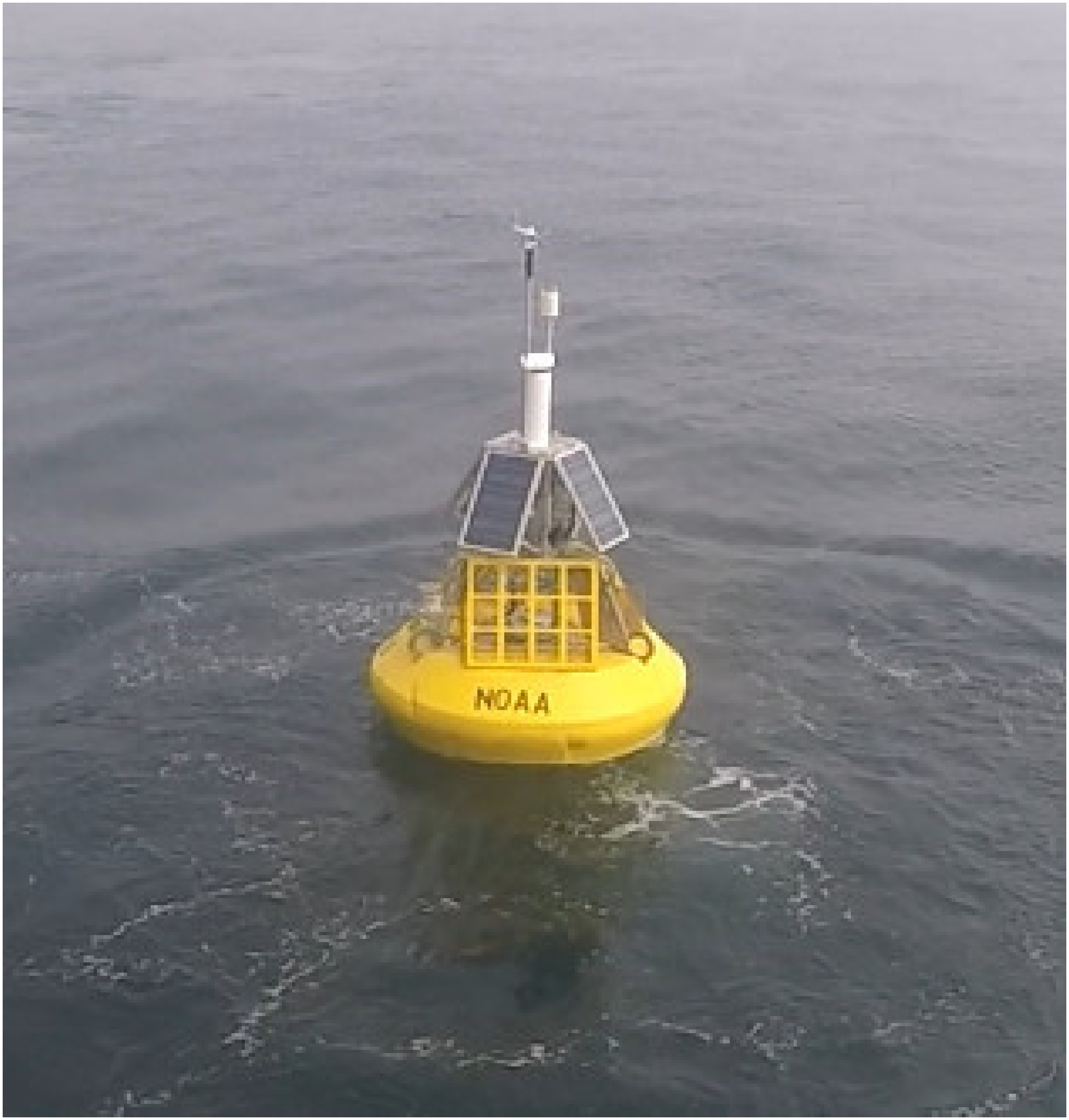
This section will present the calculations pertaining to the probability distribution tails of the $H_S$ variable. These calculations are based on a dataset obtained from wave measurements conducted at the NDBC Station 46053. The NDBC station 46053 is a buoy with a discus shape, measuring 3 m in diameter. The visual representation of this buoy can be observed in Figure 1. The data buoy is situated at Stonewall bank, which is located approximately 20 nautical miles to the west of Newport, within the state of Oregon in the United States. The water depth at this site is 405 m. The dataset pertaining to wave measurements was collected at hourly intervals from 1 January 1996 to 31 December 2021. It consists of 196,217 data points for significant wave heights ( $H_S$ ) and an equal number of corresponding values for energy periods ( $T_e$ ).

Figure 1.

The picture of the data buoy NDBC 46053 (https://www.ndbc.noaa.gov/station_page.php?station = 46053).

Further measurement descriptions regarding these NDBC buoy 46053 data are as follows: Real-time files generally contain the last 45 days of “Realtime” data—data that went through automated quality checks and were distributed as soon as they were received. Historical files have gone through post-processing analysis and represent the data sent to the archive centers. The formats for both are generally the same, with the major difference being the treatment of missing data. Missing data in the Realtime files are denoted by “MM” while a variable number of 9's are used to denote missing data in the historical files, depending on the data type (for example: 999.0 99.0).

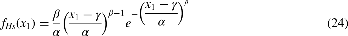
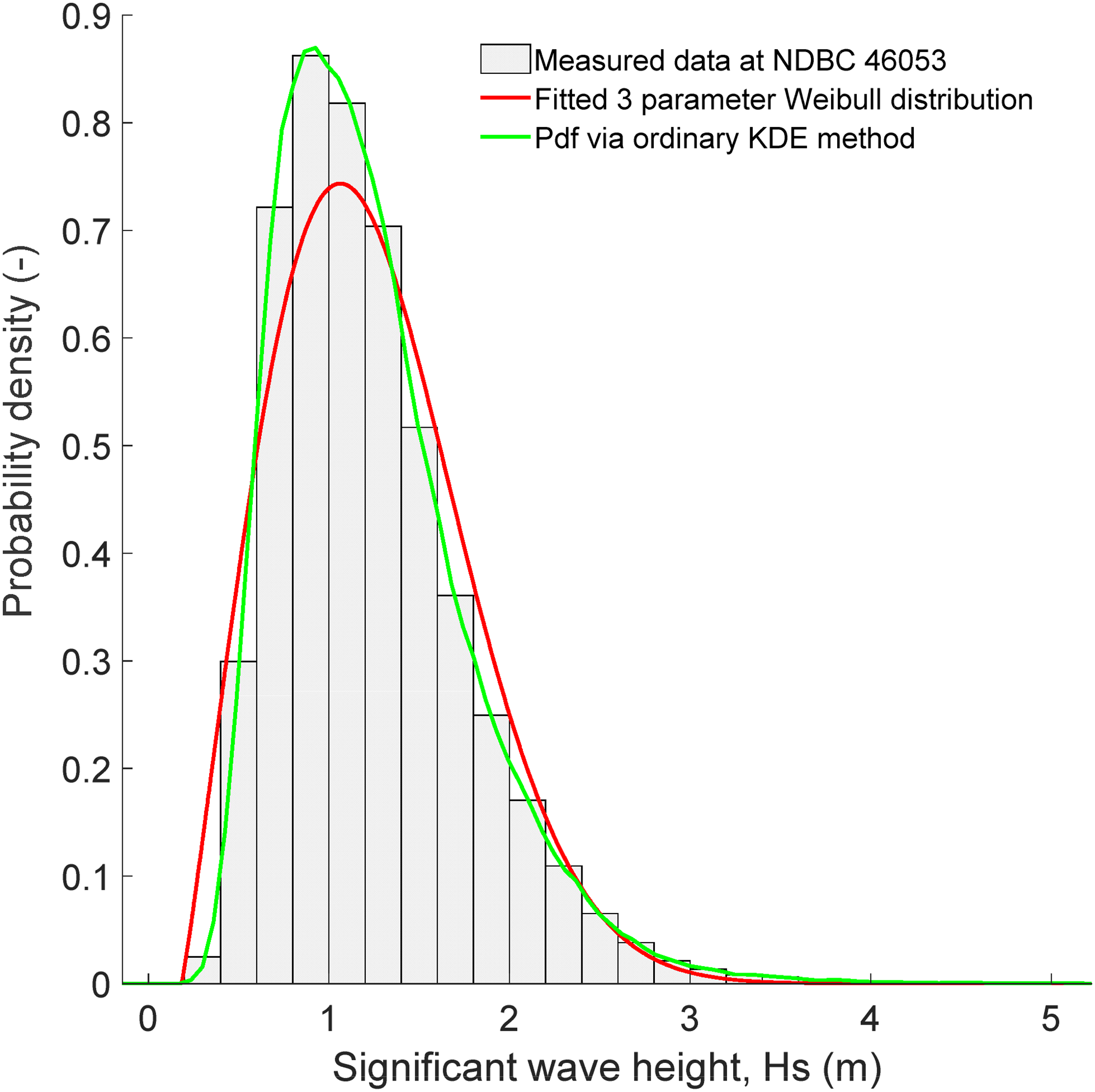
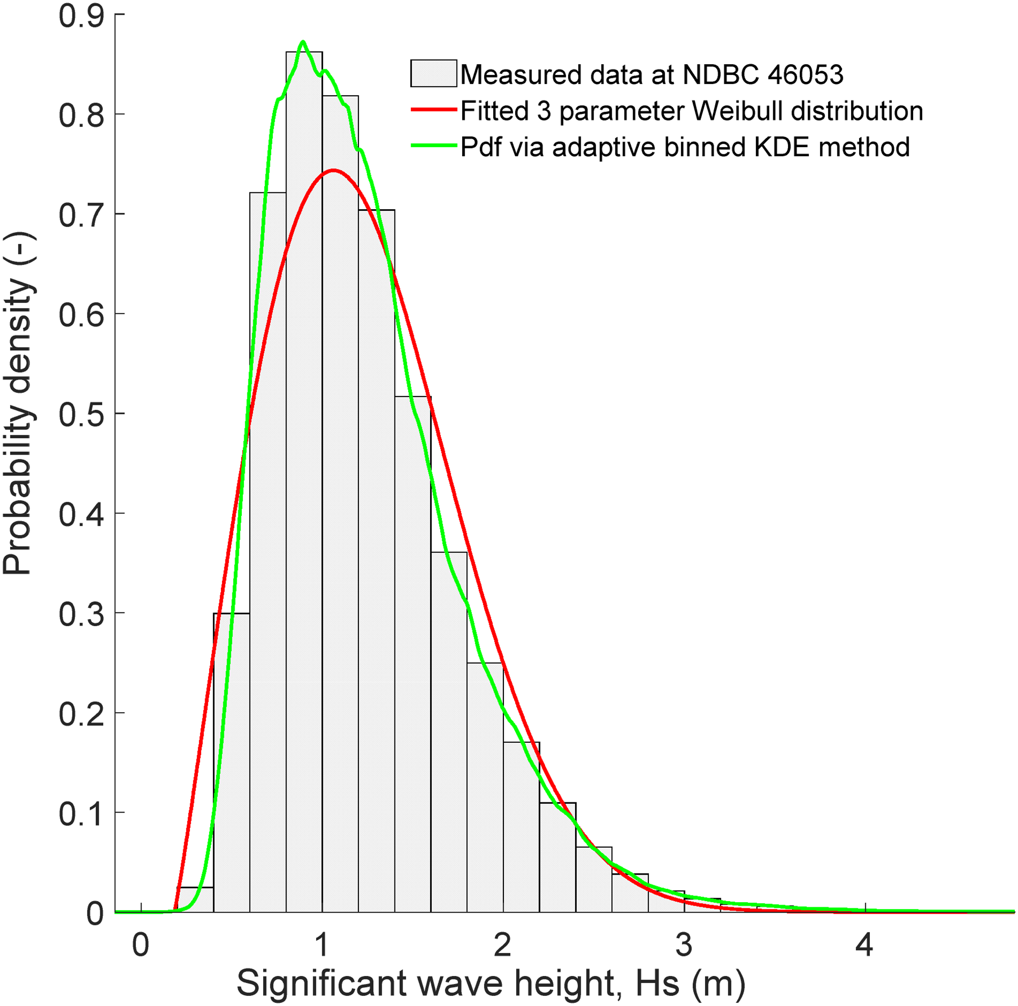
The probability density distributions calculated based on the aforementioned $H_S$ values are presented in Figure 2 in which the red curve shows the calculation results by fitting the aforementioned wave dataset to a 3-parameter Weibull model expressed as follows:

$$f_{Hs}(x_1)={\displaystyle \frac{\beta }{\alpha }{\left({\displaystyle \frac{x_1-\gamma }{\alpha }}\right)}^{\beta -1}{e}^{-{\left({\displaystyle \frac{x_1-\gamma }{\alpha }}\right)}^{\beta }}}$$

(24)

Figure 2.

Model fit between the measured data at NDBC 46053 and the two considered models respectively.

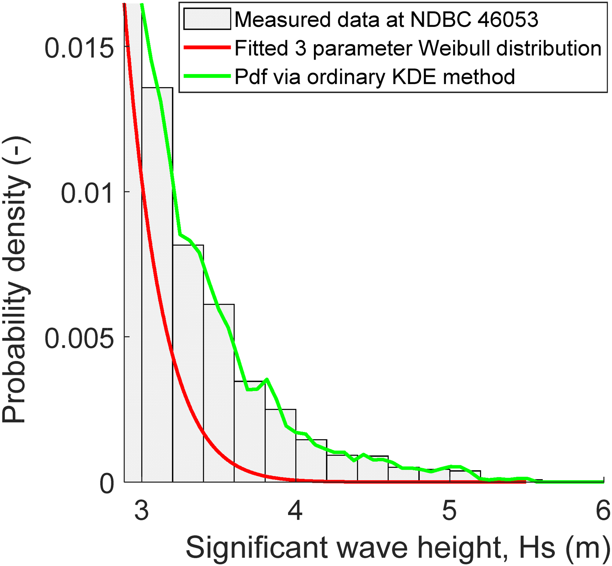
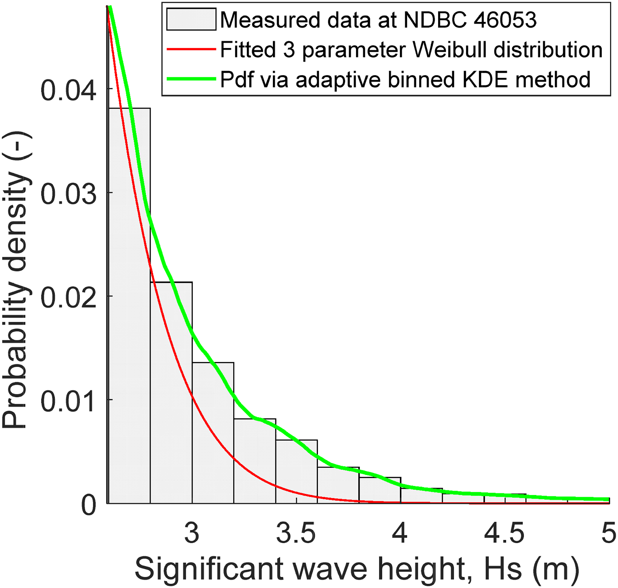
The parameters in the aforementioned model were determined using a maximum likelihood method, yielding the following values: $\alpha$ = 1.1939, $\beta$ = 2.1040, and $H_S$ = 0.1835. Upon analyzing the computational outcomes presented in Figure 2, it becomes evident that the mode of the fitted 3-parameter Weibull probability density distribution is significantly lower in comparison to the mode observed in the histogram of the measured ocean wave dataset. To examine the efficacy of the 3-parameter Weibull model in accurately fitting the tails of the probability density distribution, a detailed plot was generated and is depicted in Figure 3. Upon analyzing the computational outcomes depicted in Figure 3, it becomes evident that the fitted 3-parameter Weibull probability density distribution exhibits significantly lower values in the tail region compared to the histogram representing the measured ocean wave dataset. The obtained calculation results unequivocally indicate that the utilization of the parametric 3-parameter Weibull model is not suitable for accurately fitting the probability density distribution of $H_S$ .

Figure 3.

Model fit at the tail region between the measured data at NDBC 46053 and the two considered models respectively.

The green distribution curve depicted in Figure 2 represents the results of the calculation obtained by applying the ordinary KDE method to fit the wave dataset mentioned earlier. Upon analysis of the computational outcomes presented in Figure 2, it is evident that the mode of the ordinary KDE probability density distribution closely aligns with that of the histogram representing the observed ocean wave dataset. To examine the efficacy of the ordinary KDE technique in modeling the tails of the probability density distribution, the aforementioned zoom-in plot depicted in Figure 3 was employed once more. Upon analyzing the computational outcomes depicted in Figure 3, it becomes apparent that the ordinary KDE distribution curve exhibits a zigzag pattern within the tail region. The obtained calculation results provide clear evidence that the ordinary KDE method is not a suitable option for accurately fitting the $H_S$ probability density distribution.

In order to enhance computational accuracy and efficiency, the proposed new adaptive binned KDE method has been employed to forecast the tails of the $H_S$ probability density distribution. The calculation was conducted using the afore-mentioned set of measured wave data, and the computational outcomes are depicted in Figure 4 as the probability density distribution represented by the green curve.

Figure 4.

Model fit between the measured data at NDBC 46053 and the two considered models respectively.

Through an analysis of the computational outcomes depicted in Figure 4, it becomes evident that the mode of the newly proposed adaptive binned KDE probability density distribution (represented by the green curve) closely aligns with the mode of the histogram derived from the observed ocean wave dataset. To examine the efficacy of our proposed adaptive binned KDE method for modeling the tails of the probability density distribution, the zoom-in plot depicted in Figure 5 was employed. Upon analyzing the computational outcomes depicted in Figure 5, it is evident that the newly proposed adaptive binned KDE distribution curve exhibits a high degree of smoothness and effectively aligns with the histogram of the recorded ocean wave dataset, particularly in the tail region. An interpretation of this result is that these accurate tail distribution results will lead to a more accurate 50-year environmental contour line from which several more accurate extreme sea states can be selected. The subsequent dynamic analysis of a WEC based on these selected extreme sea states will yield more accurate long-term response values. In addition, the computational efficiency of running the MATLAB program to generate the green curve in Figure 4 on the Dell Precision 5820 high-performance tower desktop workstation previously mentioned was notable, with a runtime of approximately 4 s. These reveal the phenomenon and mechanism that the proposed adaptive binned KDE method is a preferable option for accurately capturing the distribution tails of sea state parameters and predicting the extreme dynamic responses in time-constrained real-world engineering projects.

Figure 5.

Model fit at the tail region between the measured data at NDBC 46053 and the three considered models respectively.

Calculation examples regarding the 50-year environmental contour lines

The predicted 50-year environmental contour lines based on the aforementioned measured NDBC 46053 data are summarized as follows:

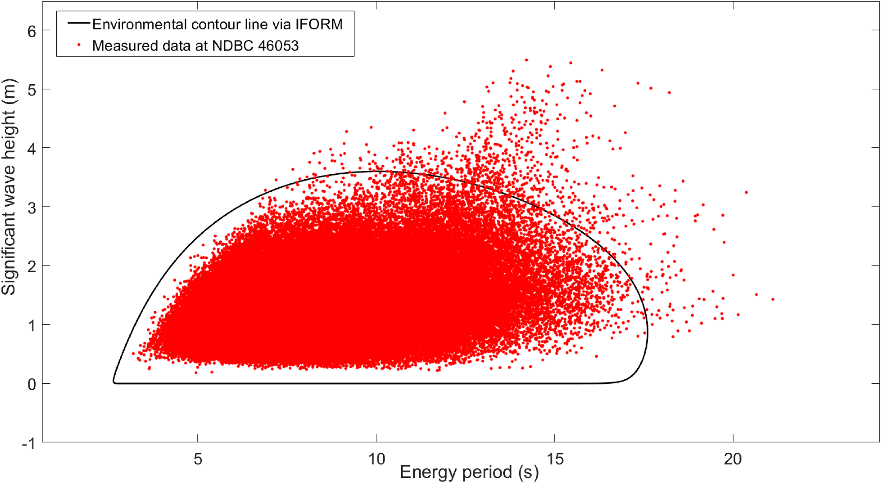
Figure 6 contains a total of 196,217 red “dots,” wherein each dot represents a measured $H_S$ value and its corresponding $T_e$ value at the previously mentioned NDBC station 46053. A total of 196,217 hourly measurements of $H_S$ and $T_e$ were collected over the time period spanning from 1 January 1996 to 31 December 2021. The derivation of the black Rosenblatt-I-FORM environmental contour line was based on the mathematical theories discussed in section “The theoretical backgrounds of the I-FORM and I-SORM environmental contour line approaches.” To be more specific, the initial stage in the process of obtaining the black contour was to fit the observed 196,217 $H_S$ values with a 3-parameter Weibull probability density distribution. In addition to this, it was necessary to fit the measured 196,217 $T_e$ values with a conditional lognormal distribution. After that, the equations (1) to (4) in section “The theoretical backgrounds of the I-FORM and I-SORM environmental contour line approaches” were used to derive the black Rosenblatt-I-FORM environmental contour shown in Figure 6.

Figure 6.

The 50-year environmental contour line created by the traditional I-FORM method for NDBC 46053.

A 50-year environmental contour ought, according to the presumption of common sense, to include the majority of the 26-year wave data observed at the NDBC station 46053 that was described before. Nevertheless, a surprisingly significant number of observed data points with high $H_S$ values have exceeded the black Rosenblatt-I-FORM environmental contour line. This was an unexpected finding. This suggests that the black Rosenblatt-I-FORM contour will produce results that are not conservative and will lead to the design of offshore renewable energy systems that are not safe.

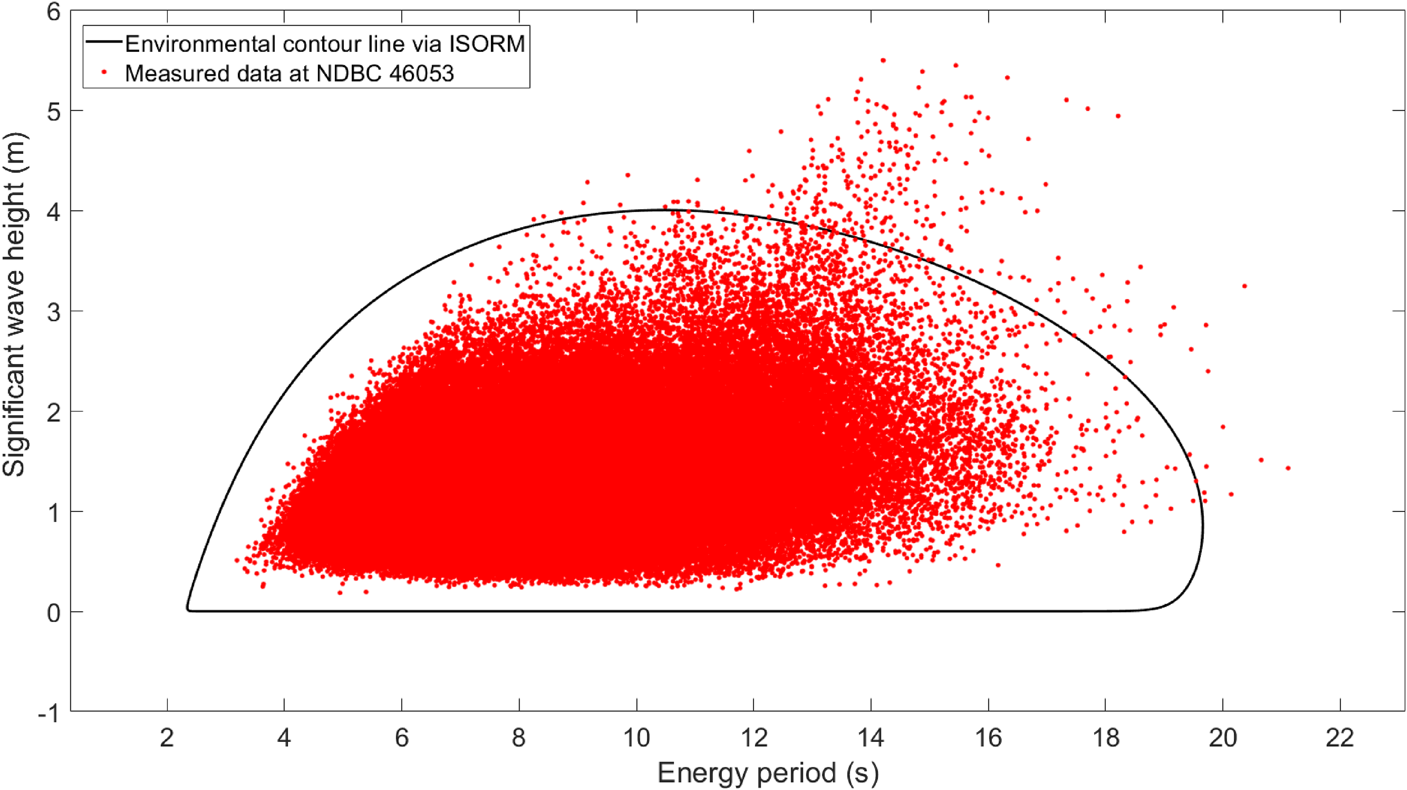
In a similar vein, Figure 7 displays a total of 196,217 red “dots,” with each dot symbolizing a measured $H_S$ value and its corresponding $T_e$ value at the previously mentioned NDBC station 46053. A total of 196,217 hourly measurements of $H_S$ and $T_e$ were collected over the time period spanning from 1 January 1996 to 31 December 2021. The derivation of the black Rosenblatt-I-SORM contour depicted in Figure 7 was conducted using the equations (1) to (5) presented in section “The theoretical backgrounds of the I-FORM and I-SORM environmental contour line approaches”. In theory, the Rosenblatt-I-SORM approach is more conservative than the Rosenblatt-I-FORM method. This theory is supported by the observation that the I-SORM contour in Figure 7 has missed less of the recorded wave data when compared to the Rosenblatt-I-FORM contour in Figure 6. However, a closer examination of Figure 7 reveals that the Rosenblatt-I-SORM environmental contour line is still surpassed by a number of measured wave data points having high $H_S$ values. This suggests that the Rosenblatt-I-SORM environmental contour line will also produce unconservative results and contribute to the design of insecure offshore renewable energy systems.

Figure 7.

The 50-year environmental contour line created by the traditional I-SORM method for NDBC 46053.

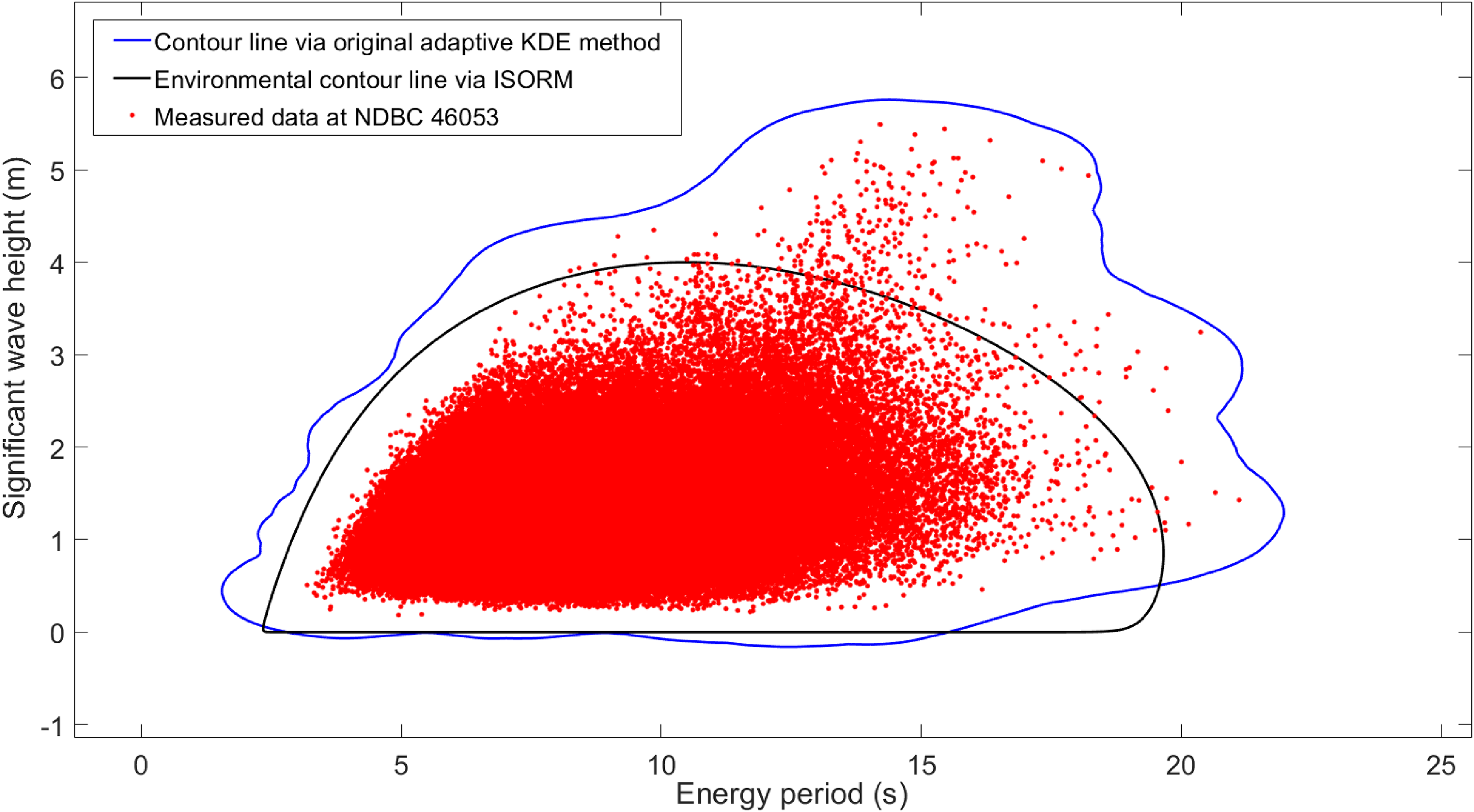
Due to dissatisfaction with the outcomes obtained through the utilization of the I-FORM and I-SORM techniques, which rely on fitted parametric distributions of sea state parameters, it was endeavored to employ the original adaptive KDE method in order to derive the environmental contour line. The computational findings are depicted in Figure 8. The 50-year environmental contour line, obtained through the utilization of the original adaptive KDE method, is represented by the blue curve in Figure 8. Evidently, the blue curve exhibits a strong adherence to the profile of the measured data set, encompassing nearly all of the data points. It is evident that the blue environmental contour line in Figure 8 is expected to outperform the black environmental contour line in terms of its efficacy in predicting the extreme values of the dynamic responses of WECs. Regrettably, the execution of the MATLAB code on a Dell Precision 5820 high performance tower desktop workstation requires a duration exceeding 3440 s in order to obtain the blue curve depicted in Figure 8. The computational cost of this approach is prohibitively high, particularly in the context of time-sensitive engineering projects. In order to get better results for the 50-year environmental contour lines, the proposed new adaptive binned KDE approach had subsequently been resorted to in this work in order to overcome this deficiency of the original adaptive KDE method. This was done in an attempt to overcome this deficiency of the original adaptive KDE method. The results of the corresponding calculations have been acquired by executing a program in MATLAB, and they have been depicted in Figure 9 as the green environmental contour line.

Figure 8.

50-year extreme sea state contours created by the traditional method and the original adaptive KDE method presented in this paper for NDBC 46053.

Figure 9.

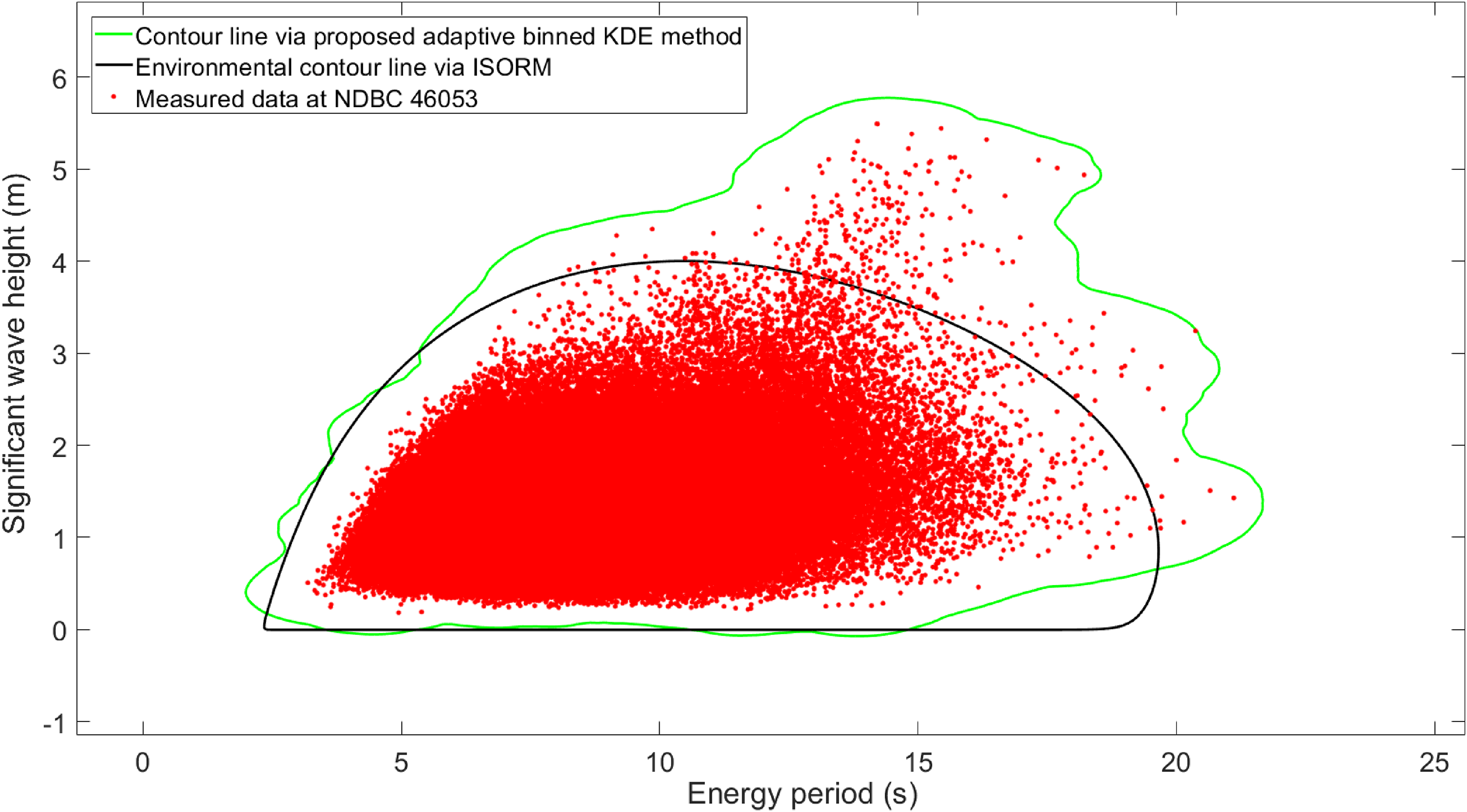
50-year extreme sea state contours created by the traditional method and the proposed new adaptive binned KDE method presented in this paper for NDBC 46053.

It is worth noting that the effectiveness of our proposed adaptive binned KDE method in predicting the $H_S$ (or $T_e$ ) probability distribution tail has been demonstrated in Figures 4 and 5. Furthermore, the accuracy of the green environmental contour line, as depicted in Figure 9, can be attributed to its direct derivation from the nonparametric KDE $H_S$ and $T_e$ probability distributions. In contrast, the black Rosenblatt-I-SORM contour, which is derived from the parametric $H_S$ and $T_e$ models with inaccurate probability distribution tails, is less accurate. The green curve exhibits a strong adherence to the profile of the measured data set, encompassing nearly all of the data points. Remarkably, the acquisition of the green curve depicted in Figure 9 necessitates a mere 255 s of computational time when executing the MATLAB code on a Dell Precision 5820 high-performance tower desktop workstation. This suggests that the green environmental contour, which is obtained through the newly proposed adaptive binned KDE method, is expected to outperform the black Rosenblatt-I-SORM contour. Consequently, this advancement could contribute to the development of offshore sustainable energy systems that are both secure and dependable.

The extreme dynamic responses of a specific offshore sustainable energy system

The selected offshore sustainable energy system

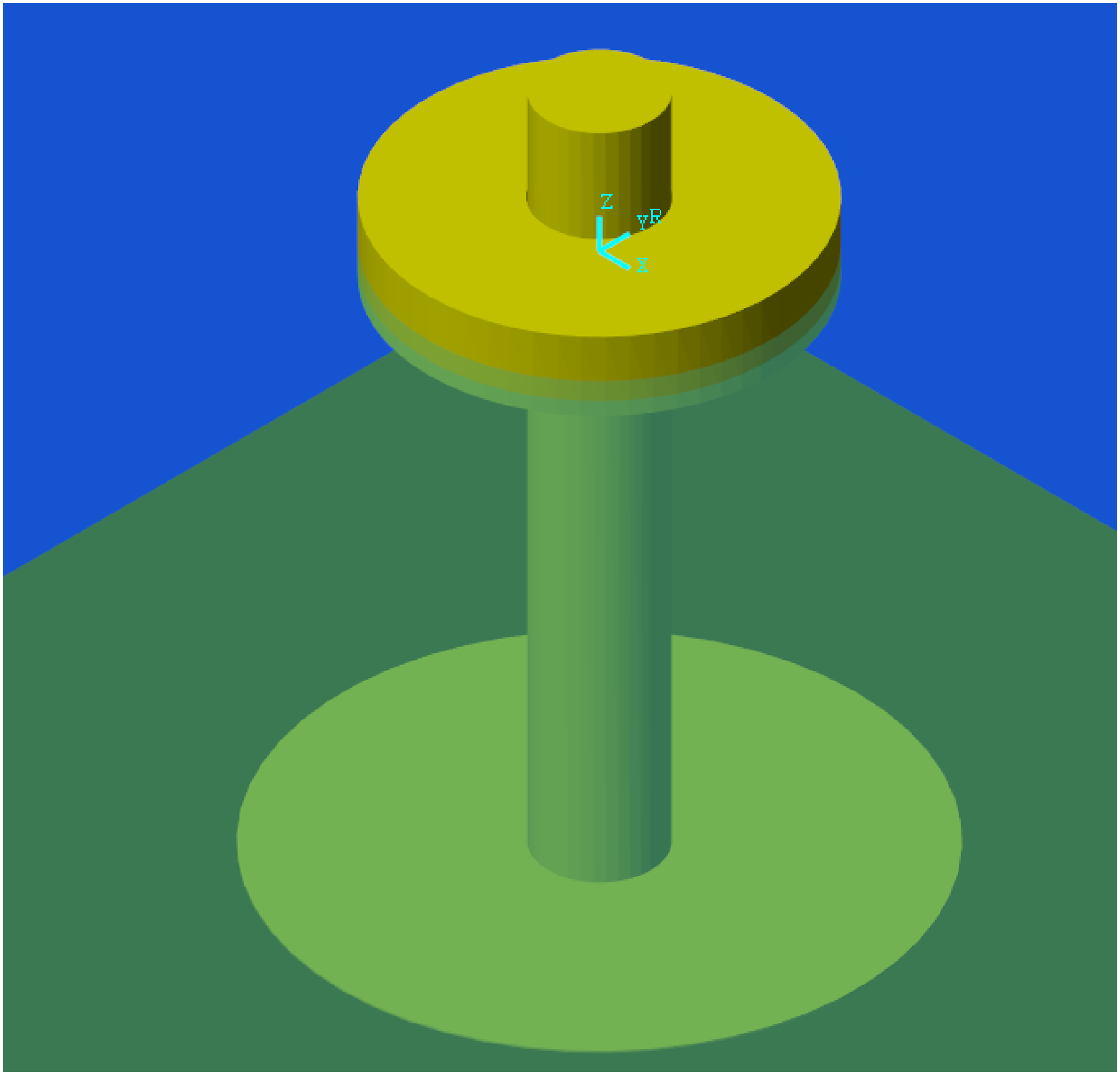
In this study, a particular offshore sustainable energy system was selected, namely a two-body floating point absorber WEC. The WEC simulation model was developed utilizing the open-source software WEC-Sim (https://wec-sim.github.io/WEC-Sim/master/introduction/overview.html). The visual representation of this model is presented in Figure 9. WEC-Sim, also known as Wave Energy Converter SIMulator, is a freely available software tool designed for the purpose of simulating WECs. The software implementation is carried out in MATLAB/SIMULINK, utilizing the Simscape Multibody solver for multi-body dynamics analysis. WEC-Sim possesses the capability to simulate devices consisting of hydrodynamic bodies, joints and constraints, power take-off systems, and mooring systems. The time-domain simulations involve the solution of the governing equations of motion for WECs in the 6 rigid Cartesian degrees-of-freedom (Figure 10).

Figure 10.

The WEC-Sim simulation model of the selected floating WEC.

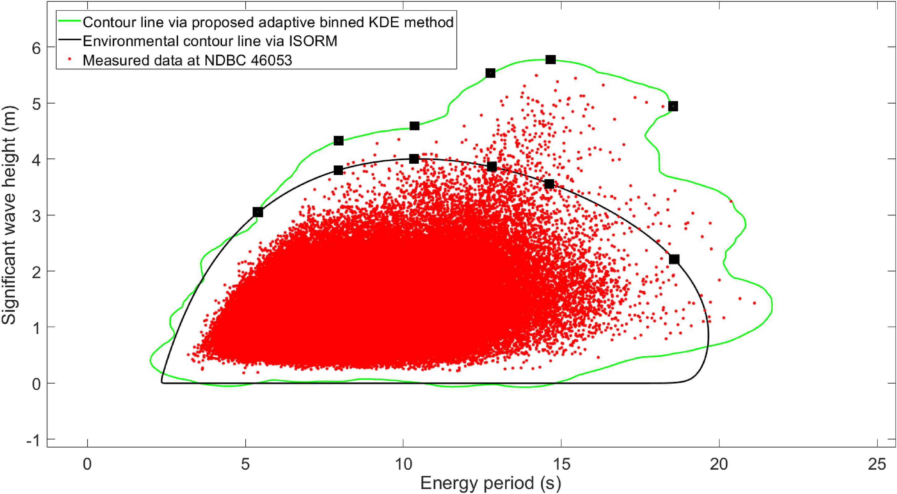
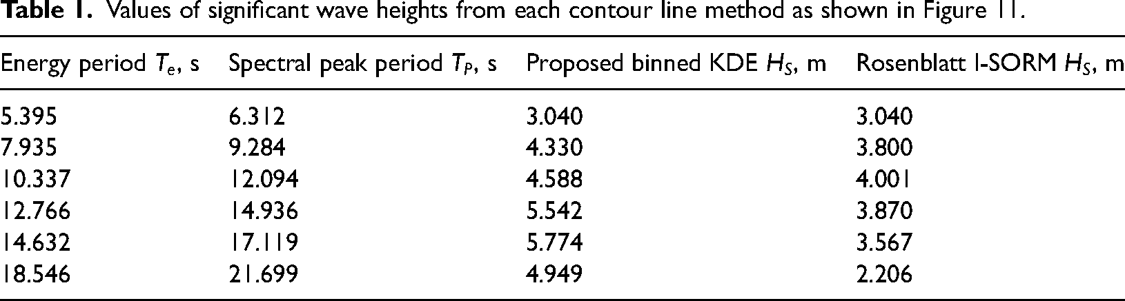
The offshore sustainable energy system under consideration comprises a spar with a diameter of 6 m and a float with a diameter of 20 m. The spar has been specifically engineered with a vertical dimension of 38 m and a weight of 878.3 metric tons. The float has been engineered to possess a thickness of 5 m and a mass of 727.01 metric tons. The installation of this particular offshore sustainable energy system takes place at an oceanic location characterized by a water depth of 82 m. Dynamic simulations using WEC-Sim have been conducted to predict the 50-year extreme PTO heaving forces of the floating WEC in six selected fully developed sea states. These sea states are characterized by a Pierson-Moskowitz ocean wave spectrum. A set of six $T_e$ values representing fully developed sea states were chosen for each of the two contours depicted in Figure 11. These $T_e$ values are as follows: 5.395, 7.935, 10.337, 12.766, 14.632, and 18.546 s. This set of six $T_e$ values has been chosen in order to encompass the highest $T_e$ values. The black solid squares in Figure 11 represent the chosen fully developed sea states, while Table 1 provides a summary of the corresponding values of the parameters associated with these sea states.

Figure 11.

50-year extreme sea state contours created by the traditional method and the proposed new adaptive binned KDE method presented in this paper for NDBC 46053.

Table 1.

Values of significant wave heights from each contour line method as shown in Figure 11.

Energy period $T_e$ , s	Spectral peak period $T_P$ , s	Proposed binned KDE $H_S$ , m	Rosenblatt I-SORM $H_S$ , m
5.395	6.312	3.040	3.040
7.935	9.284	4.330	3.800
10.337	12.094	4.588	4.001
12.766	14.936	5.542	3.870
14.632	17.119	5.774	3.567
18.546	21.699	4.949	2.206

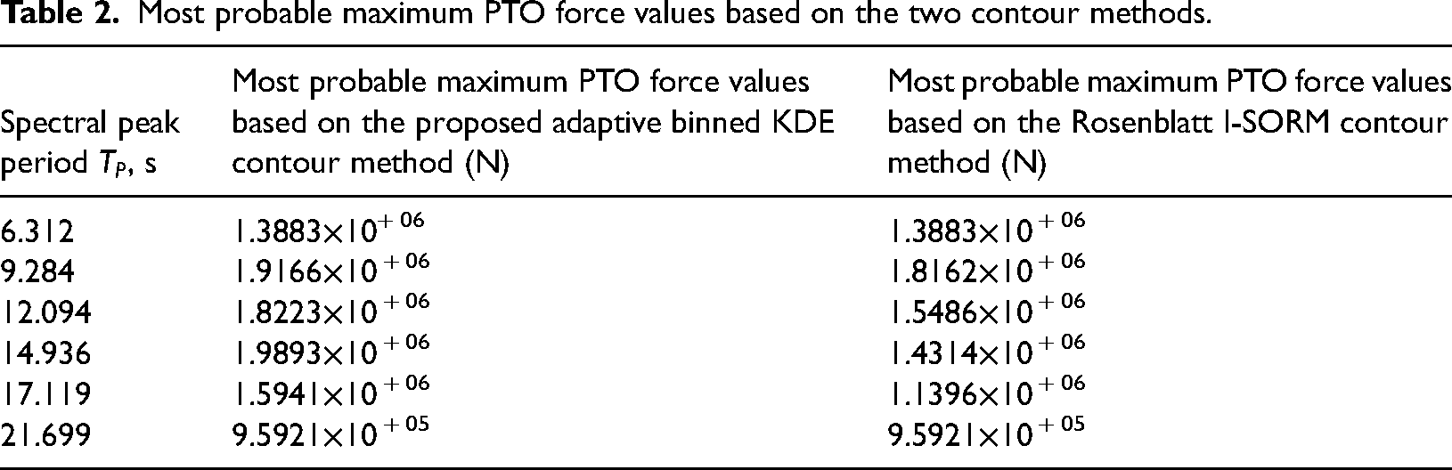
These particular fully developed sea states, each of which was defined by a unique Pierson-Moskowitz ocean wave spectrum, were used as inputs for the time-domain simulations carried out by WEC-Sim in order to determine the WEC dynamic responses based on the theories described in section “Theories for the dynamic analysis of an offshore sustainable energy system.” One particular category of dynamic responses, specifically the three-hour time series of the PTO heaving forces, has been collected. It is essential to account for these PTO heaving forces while building the floating WEC. After that, a most probable maximum value corresponding to each 3-h time series of the PTO heave forces was estimated with the help of the theories that were elaborated on in Edwards et al. (2019). After performing this technique for all of the previously indicated six $T_e$ values for each of the two environmental contours depicted in Figure 11, this paper was able to acquire all of the most probable maximum PTO heave force values, which are listed in Table 2.

Table 2.

Most probable maximum PTO force values based on the two contour methods.

Spectral peak period $T_P$ , s	Most probable maximum PTO force values based on the proposed adaptive binned KDE contour method (N)	Most probable maximum PTO force values based on the Rosenblatt I-SORM contour method (N)
6.312	1.3883×10+ 06	1.3883×10 + 06
9.284	1.9166×10 + 06	1.8162×10 + 06
12.094	1.8223×10 + 06	1.5486×10 + 06
14.936	1.9893×10 + 06	1.4314×10 + 06
17.119	1.5941×10 + 06	1.1396×10 + 06
21.699	9.5921×10 + 05	9.5921×10 + 05

A meticulous examination of the data presented in column 2 of Table 2 elucidates that the highest recorded value among the six most probable maximum PTO heaving force values, as determined by the newly proposed adaptive binned KDE technique, amounts to 1989300N. This particular value is identified as the 50-year extreme PTO heaving force value. In a similar vein, an examination of the data in column 3 of Table 2 uncovers that the predicted 50-year extreme PTO heaving force value, as determined by the Rosenblatt-I-SORM contour method, amounts to 1816200N. This value is significantly lower than the 1989300N value predicted by the new method. Consequently, this discrepancy has the potential to compromise the safety of the design for an offshore sustainable energy system, specifically a floating WEC, as explored in this study. The aforementioned results indicate that the proposed novel adaptive binned KDE technique exhibits strong predictive capabilities and efficiency in estimating the 50-year extreme design force values for offshore sustainable energy systems.

Finally, it should be noted that the proposed novel adaptive binned KDE method has been verified based on an ocean wave dataset measured at NDBC buoy 46053. Obviously, this adaptive binned KDE method can also be verified based on a hindcast simulated dataset that has the same data format as that of the measured buoy data. Consequently, the universality of the proposed novel adaptive binned KDE method can be ensured.

Conclusions

During the course of this study, the author came up with a new method for the adaptive binned KDE. A description of the new method is as follows: It is noted that the kernel estimate is a convolution of the data with the kernel. In the proposed new method, Fourier transforms have been utilized to accomplish the convolution rather than performing the convolution by hand. By utilizing the FFT, direct and inverse Fourier transforms have been found in a relatively short amount of time when implementing the new method.

When the results of the calculations were examined, it was seen that in the tail area, the suggested new adaptive binned KDE distribution curve becomes quite smooth and fits pretty well with the histogram of the recorded ocean wave dataset at the NDBC station 46053. These are the major advantages of our proposed new method comparing with other existing methods such as the parametric method, the ordinary KDE method and Abramson's adaptive KDE method. The specific research gap identified in the field is that none of the existing methods can predict the sea state parameter probability distribution tails both accurately and efficiently, and the proposed new method has successfully addressed this research gap. Studying the calculation results in great detail also indicates that the value predicted for the 50-year extreme PTO heave force based on the environmental contour generated using the new method is 1989300N. This value is significantly higher (by more than 9.5%) than the figure 1816200N that was forecasted using the Rosenblatt-I-SORM contour method. The author has come to the conclusion that the new adaptive binned kernel density estimate approach that has been suggested is reliable and has the ability to accurately predict the values of the 50-year extreme design force for WECs.