Sage Journals: Discover world-class research

Abstract

In this paper genetic algorithm (GA) was used for the optimization of two natural gas network, the study focuses on fuel consumption minimization of the second gas network. Studies using GA to simultaneously optimize a gas network and a compressor station based on the constraint of the gas network and compressor station are limited. The relationship between several compressor speed and the total fuel consumption and the relationship between the sum of pressure drop in compressor station loops and compressor inlet flow are assessed for optimization. For this purpose, the optimization of two networks was presented and the results were compared with result from analytical methods. The first network problem was to determine the flow rates and node pressures under a given load, which serves as a guide in using GA. Comparison with result from analytical solution showed good agreement of predicted values. The second network consisted of two compressor stations, each containing six compressors with the objective to optimize the fuel consumption of the system. The simulation was divided into two main simulations, the first simulation was the flow optimization, which results in the optimum flow, based on the fitness function, which is the summation of pressure loss for each compressor station. In the second simulation which was the speed optimization, the optimum set of compressor speed was obtained which depends on the fitness function, which is the minimum fuel consumption, the flow obtained from the flow optimization served as input and remained constant. All speeds were simulated together. The predicted results were compared with literature and showed GA can be used for compressor station fuel optimization but still requires improvement. Based on the outcomes, data on natural gas network operations should be accessible to encourage studies on fuel consumption and CO₂ emissions minimization.

Keywords

Genetic algorithm compressor station fuel consumption flow optimization speed optimization encoding genes

Introduction

Natural gas is a volatile, flammable, relatively clean, compressible fossil fuel (FF) often isolated and kept at the minimum pressure required for appliances, Squire Energy (2017). Natural gas is the cleanest FF which is expected to become the dominant FF due to a shift to cleaner energy. Global demand for natural is expected to keep growing until 2035 at the height of its demand. Within the various consumers of natural, it is expected that the power generation sector will be the principal consumer of natural gas, followed by the manufacturing sector or the building sector, with the least consumption in the transport sector due to electrification and increased energy efficiency, DNV GL (2017). During production, crude oil flows from the reservoir to the wellbore where flow is controlled with the choke valve, and sent to the separator, resulting in oil, water, and gas fluids. Gas streams are sent to a processing facility for treatment, after which, its recompressed and sent to the transmission pipe, Allison et al. (2019). Natural gas is transported mostly by pipeline reaching thousands of kilometers across international borders, where great distance covered leads to significant pressure loss, resulting in an inadequate flow and insufficient pressure. 8The transportation of gas from the processing facility to the user appliances is possible through a gas network, which comprises a source, various pipes, intersections between pipes also known as nodes, compressors, a group of compressors also referred as a compressor station, control valves, and load (demand). Pressure losses occur at the pipe because of control valve operation, viscosity, pipe roughness, friction, temperature, and changes in pipe diameter and elevation.

Pressure loss is minimized by compression at optimum locations with a compressor. Compression may be required at various stages as illustrated in Figure 1. Compression is conducted by gas or electrically powered compressor due to its driver, such as a gas turbine or electric motor. Multiple compressors are combined in a compressor station to obtain greater flow or pressure in a parallel or serial arrangement, respectively. Compressors are classified into two main groups, positive displacement compressors, and dynamic compressors, positive displacement compressors operate on a trapped volume of gas, while dynamic compressors operate by continuously increasing the momentum of gas flow through them, examples of positive displacement compressors include reciprocating compressors and screw compressors, while dynamic compressors include centrifugal, axial, and mixed flow compressors, Hoopes et al. (2019). The operation of compressor station consumes about 2 to 5 percent of the natural gas from the pipe, optimization of a compressor station reduces fuel consumption cost and carbon dioxide emission.

Figure 1.

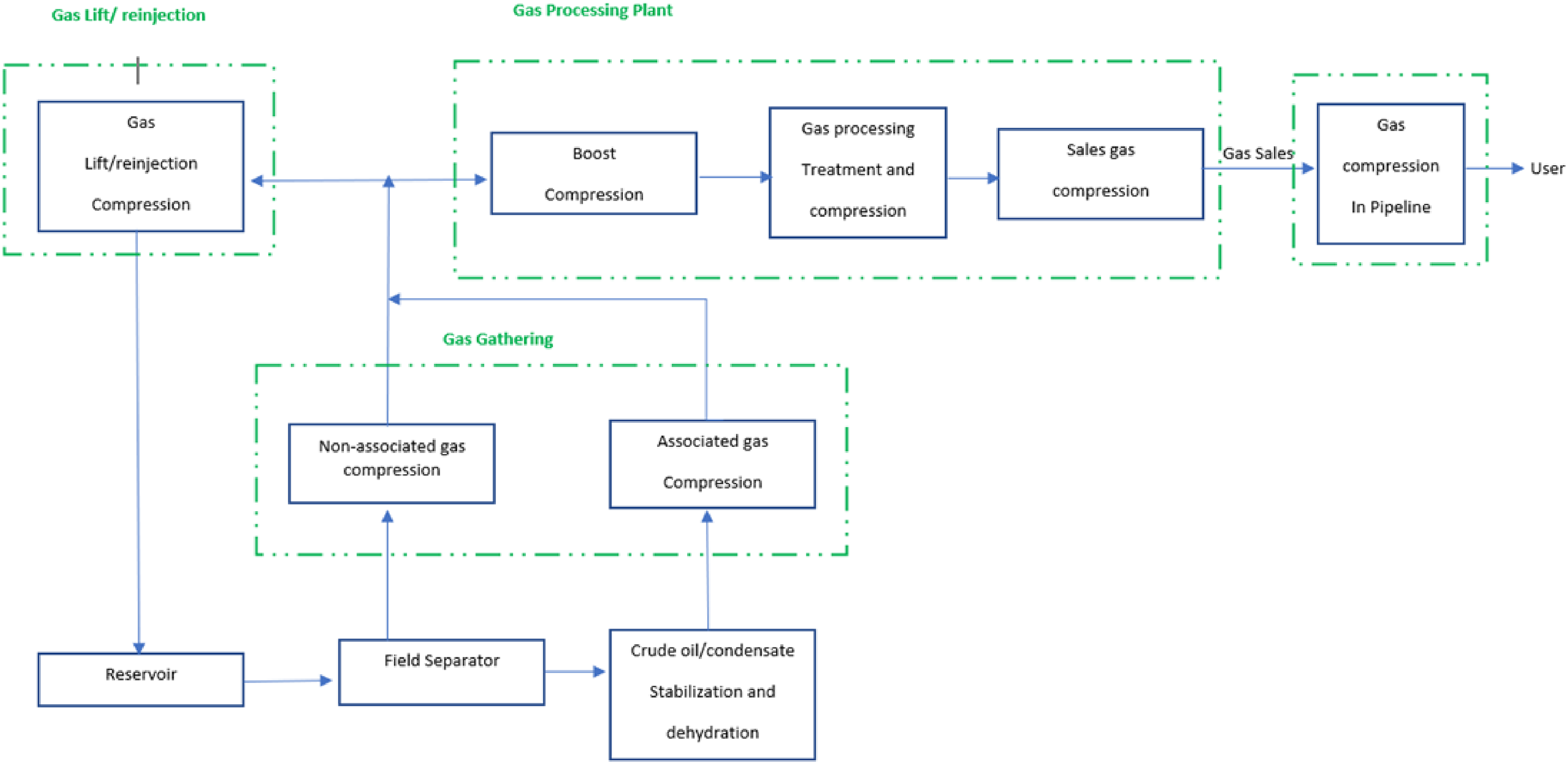
Compression applications from Allison et al. (2019).

Carbon dioxide emissions leads to more greenhouse gases, which is responsible for global warming. The United Nations (2015) documented the Paris agreement which is the framework that unites developed and developing nations to address the challenges of climate change and to work according to their capacity on controlling their emissions of greenhouse gases to acceptable levels. The Paris agreements are defined by its articles, several articles relating to its goals and approach in addressing environmental deterioration are as follows:

Article 2 states that the global temperature should not be allowed to rise above 2°C above pre-industrial levels and supporting efforts should restrict the temperature increase to 1.5°C above pre-industrial levels.

Under article 4 and in its introduction, it states that, achieving the long-term temperature goal is maintained by reaching the global peak of greenhouse gas emissions in the fastest time and there after undertaking rapid reductions in greenhouse gas emission, understanding that peaking will take longer for developing country, with consideration to equity, sustainable development, and efforts on poverty eradication.

Under article 5, subsection one, parties should take action to conserve and enhance, as appropriate, sinks and reservoirs of greenhouse gases as referred to in article 4.

Article 9 states that developed country shall provide financial resources to assist developing country with respect to both mitigation and adaptation.

Article 10 subsection one states that members should encourage technological development and transfer, subsection five, states that members should encourage and accelerate innovation towards climate change and promoting economic growth and sustainable development. Subsection six states that financial support should be provided for developing countries for technology development and transfer at various stages of the technology cycle.

Studies on environmental deterioration measure the effects of the factors contributing to the deterioration in the air, land, and water. Environmental deterioration is usually indicated by terms such as CO₂ emissions, load capacity factor (LCF) and the ecological footprint. Several studies conducted on environmental deterioration are mentioned subsequently. For example, Xu et al. (2022) utilized the autoregressive distributed lag (ARDL), dynamic ARDL, and Breitung Candelon causality tests to assess the effect of technological innovation, economic growth, structural change, and nonrenewable energy use on CO₂ emissions in Turkey using a yearly dataset spanning between 1980 and 2019. The outcomes of the dynamic ARDL disclosed that economic growth and nonrenewable energy use contribute to the degradation of the environment, while technological innovation improves the quality of the environment. The outcome also shows that economic expansion is one of the nation's largest sources of CO₂ emissions which might be due to Turkey's goal of becoming a fully developed nation, which has resulted in an emphasis on rapid economic expansion rather than environmental protection. Other contributors to CO₂ emissions include lax ecological laws in the industrial system, a greater emphasis on oil and coal for economic operations instead of cleaner sources of energy. Similarly, Adebayo et al. (2022a) assessed the influence of agriculture, financial development, economic growth, urbanization, and Renewable energy (REC) on CO₂ emissions in Turkey using quarterly data stretching from 1985 to 2019. The assessment was carried out using econometric techniques such as non-parametric Granger causality and quantile-on-quantile regression (QQR) to determine how the quantiles of the independent variables affect the quantiles of CO₂ emissions. The outcomes from the QQR show that in all quantiles, financial development, economic growth, urbanization, and agriculture impact CO₂ emissions positively (increases CO₂₎, while in the middle quantiles, the influence of REC use on CO₂ is negative (reduces CO₂₎. Moreover, Adebayo et al. (2022b) utilized the nonlinear autoregressive distributed lag (NARDL) to capture the nonlinear impact of economic growth, globalization, and technological innovation on CO₂ emissions in Sweden by utilizing data from 1980 to 2018. The outcome of the NARDL study showed that a positive shock in GDP decreases CO₂ emissions in Sweden. Furthermore, a positive shock in globalization leads to an upsurge in CO₂. Nonetheless, a negative shock in globalization exerts an insignificant influence on CO₂. This simply implies that globalization contributes to the degradation of the environment. Moreover, from their model, it was shown that a positive variation in technological innovation decreases CO₂ emissions in Sweden. This suggests that technological innovation reduces environmental degradation in Sweden, due to many eco-innovative solutions in Sweden.

Similarly, Adebayo (2022) investigated the environmental deterioration by studying the relationship between LCF and several factors such as FF, REC, economic complexity (ECI) and foreign direct investment (FDI) in Spain utilizing a dataset covering the period between 1970Q1 and 2017Q4. The wavelet coherence (WTC) method was used in this study to capture the variables co-movement at various period. Adebayo (2022) used the LCF as a distinct proxy for ecological deterioration as recommended by Fareed et al. (2021), for measuring the elasticity of the components impacting the wellness of the environment. The outcome of the WTC method showed that in the short and medium term, REC enhances the quality of the environment except for the long term. In the short, medium, and long term, FF has a negative relationship with the LCF, indicating fossil degrades the quality of the environment. FDI has a positive relationship with LCF, indicating that FDI improves the quality of the environment. In the short, medium, and long term (periods), there is a negative connection between ECI and LCF, implying that ECI harms the quality of the environment in all periods. Finally, Awosusi et al. (2022) investigated the impact of technological innovation, globalization, non-renewable energy utilization, economic growth, and political risk on the ecological footprint in the BRICS economies by employing a dataset covering the period between 1990 and 2017 using panel quantile regression method, and based on the outcomes, policies on Environmental sustainability were designed. The outcome showed that GDP impacts positively on ecological footprint and is statistically significant across all quantiles (0.1 to 0.9). This outcome suggests that economic expansion has a positive effect on ecological footprint in the BRICS economies. Non-renewable energy usage has a positive and significant impact on ecological across all quantiles, indicating that the usage of FF degrades the ecosystem. In addition, the effect of political risk on ecological footprint is positive and significant in the 50th, 60th, 70th, 80th and 90th quantiles. Suggesting that the BRICS economies are more politically risky, resulting in an upsurge in ecological footprint. Moreover, the effect of globalization on ecological footprint indicates a negative association across all quantiles, excluding the 10th and 20th quantiles. This suggests that environmental deterioration can be mitigated by increasing the level of globalization. Finally, the impact of technological innovation on ecological footprint is positive.

Previous studies carried out using genetic algorithm (GA) are presented as follows. For instance, Haddad et al. (2013) optimized the fifth major gas transmission pipeline of the National Iranian Gas Company (IGAT 5) with Khormoj compression station by solving a single objective optimization for the compression station using GA with detailed models of the performance characteristics of compressors. The single objective optimization represents a single function that includes two control variables namely, the compressor load sharing in terms of the volume flow split to each compressor unit and compressors mode (on/off). The two control variables were encoded as a chromosome resulting in thirty-three strings or genes. Khormoj compression station consist of four similar compressors in parallel, with three active compressors and the optimization resulted in a reduced fuel consumption and equal flow distribution. The optimization is based on guidelines such as the selection of the minimum and maximum gas flow for each compressor based on the surge and stone-wall lines, respectively. The compressor head and efficiency are determined by their performance curve in which head, power, or efficiency is derived from the flow rate at different revolutions per minute and compressor speeds.

Similarly, Zhang and Wu (2015) designed four GAs with different code method and code sequence to determine the feasibility of these algorithms to solve a gas network and used comparisons amongst the outcomes to rate their performances. The coding method refers to the encoding style used for the control variables such as binary coding and real coding while the coding sequence refers to the order of the variable's representation for instance for a mixed integer nonlinear programing problem the variables are represented as a sequence of real variables followed by integer variables while for a problem with equal number of real and integer variable, it is represented as an alternating sequence of each real and integer variable. The real variable is the gas flow, and the integer variable are the on/off state of the compressor. The outcome shows that the real-coded algorithms can always offer a feasible solution except for several problems, whereas the binary coded algorithms are inferior. In addition, the coding sequence of the real-coded algorithm barely influences its feasibility rate, whereas the binary coded one is severely affecting the feasibility rate. The feasibility rate of an algorithm is defined as the proportion of the runs in which it finds any feasible solution out of its total runs.

Likewise, Narváez and Galeano (2004) presented the UN-Nethyc GA to determine the optimal combinations of pipe diameter that result in an optimal distribution of fluid (water) and minimum pipe cost in a distribution network. The proposed GA allows for the sizing of liquid distribution systems that include pipelines, nodes for consumption and provision, tanks, pumping equipment, nozzles, and control valve. Comparisons were made with solutions of a classic optimization problem reported in literature which include linear programing, nonlinear programing, and simulated annealing. The results obtained with UN-Nethyc were better than other GA in literature, while the result from Eiger et al. (1994) linear programing was better with lower cost. Similarly, Djebedjian et al. (2008) developed a GA to simulate, analyze, solve, and optimize a low and medium pressure gas distribution network. The algorithm was written in C/C++ language. The developed code passes through three main stages: (a) Network graph analysis, (b) Network analysis and simulation, and (c) Network optimization. The gradient algorithm was used for the network analysis whereas the real coded GA for the optimization. Optimization involved decreasing the diameter to minimize the cost. From the outcome it was found that gradient algorithm drastically reduces computation time and GA is an efficient algorithm for finding solutions. Moreover, Osiadacz and Isoli (2020) developed a bi-criteria algorithm to optimize a high-pressured gas network by searching for a trade-off between minimization of the running costs of compressors and maximization of gas networks capacity. The algorithm was developed with a gradient projection method and a hierarchical vector optimization method. Three gas networks were optimized, and the results were compared with the results from scaler optimization and Arithmetic mean of scalar optimization. The outcome confirm that bi-criteria optimization allows for much cheaper gas transmission system management. Similarly, El-Mahdy et al. (2010) use GA to determine the optimum sizing of pipe diameters for a given looped natural gas network topology. To implement the solution, a software was developed named “GAGAS” consisting of two major modules in a graphical user interface, the first module is a simulation module. It is used to calculate the flow in each pipe element and the pressure at each internal node for a specific given pipe combination. The second module is a GA optimization module. A GA library was constructed allowing the choice between some of the genetic operators for crossover, mutation, and selection. Different GA parameters are selected, namely, the population size, the number of generations, the crossover and mutation types and probabilities, fitness function equation and selection operators. From the outcome, GA was able to optimize a looped natural gas pipe networks with optimum pipe sizing to minimize the network cost.

Likewise, Dandy et al. (1996) optimized a design for New York ground water tunnel using an improved genetic algorithm (IGA), this design serves as an extension of the preexisting tunnel. The algorithm was modified with the addition of variable power scaling of the fitness function, an adjacency mutation operator and use of gray codes. Its fitness function consists of the pipe cost and the hydraulic performance of the pipe design. The pipe cost consists of the material, construction, maintenance operation and in addition the penalty cost (penalty cost are added when the minimum pressure requirements are violated). From the outcome of the study, the IGA resulted in a significantly lower cost than simple GA. The variable exponent of the fitness function resulted in faster convergence to a solution. A low value was employed at the beginning of IGA, so the IGA can sort through the potential strengths of the ordinary strings in the early generation. The adjacency mutations are subtle disruptions of the code which permit local exploration of the solution space. Moreover, Singh and Nain (2012) used GA to optimize the design of a natural gas pipeline resulting in lower cost in setting up the network. The fitness function consists of the cost of pipe network design and hydraulic cost. The cost of pipe network design consists of material, construction, maintenance, and operation costs, as well as the penalty cost (which is applied when the pressure requirements are violated). The GA deals with a 24-bit binary string comprising the eight by three-bit substrings representing the pipe network to be optimized. The Penalty cost for each loading case taken as the product of the maximum of all the pressure head constraint violations times a specified penalty multiplier. The outcomes of the study were compared with results from complete enumeration and non-linear optimization, and it was found that, complete enumeration can only be applied to a small network unlike GA, non-linear programing can generate only one solution while GA can generate multiple solutions. Similarly, Vairavamoorthy and Ali (2005) developed a GA optimization technique for the optimal design of water distribution systems. The objective function is the minimization of capital cost, subject to ensuring adequate pressures at all nodes during peak demands. The algorithm controls the search within the solution space using a pipe index vector (PIV). The PIV is a measure of the relative importance of pipes in a network in terms of their impact on the hydraulic performance of the network. The PIV is calculated at intervals throughout the GA process, is used to exclude sections of the search space that contain impractical or infeasible designs thus guides GA to process a healthier population during its search.

Likewise, Elshiekh (2015) used GA to minimize the fuel consumption by optimizing the speed of two compressors stations each containing three compressors, the result was confirmed with results from Ling software. From the outcomes of GA and Lingo software, similar speed was obtained for the compressors in both stations. The mass flow decreased from its original value and similarly was obtained from Ling software. Moreover, Habibvand and Behbahani (2012) applied GA to optimize the Khormoj compressor station on a major transmission pipeline. It comprises three similar compressor units driven by three similar gas turbines. The station includes three aerial coolers of same sizes in series with compressors. The optimization is bounded by speed and head limitation and the fuel consumption is the sum of the three-compressor fuel consumption. The control variables employed are mass flow shared among the compressors and compressor performance curve constraints: head verse flow; efficiency verses flow; temperature verse pressure drop of aerial coolers. Similarly, Zhang and Liu (2017), noted the limitations of GA, although GA solves several solutions at a time, it is still limited by lacking an exact way to adjust the fitness values, second, early maturity leads to a locally optimal solution rather than the global solution, and third, slow convergence as it approaches the solution. Due to these limitations, they proposed, a new formula for fitness function, crossover, and mutation probability, which resulted in less calculation time and higher accuracy, they compared the modified algorithm with an unmodified GA and observed significant improvement in optimized flow. Their approach was to modify the fitness value to prevent slow convergence as it tends to the optimal solution, the modified algorithm dynamically adjusted the probability of crossover and mutation. Li et al. (2011) modified the GA into an adaptive GA, which can dynamically generate improved crossover and mutation probability.

To the best of the author knowledge this paper adds knowledge to the research by optimizing both the natural gas network and compressor operations in two main steps. In the first major step, the algorithm optimizes the network flow with GA while the compressor speed remains constant and of same value for all compressors. In the second major step GA is used to optimize all the compressor speed while the flows remain constant and are derived from the result of the first Step. Innovations of industrial production and other processes aimed at both cost and pollution minimization result in sustainable operations that maintains economic growth of the developing nations. Also ensures that current and future populations are not harmed by environmental degradation and supports the preservation of the diversity within the eco-system. Reducing the fuel consumption of a compressor station reduces CO₂ emissions, therefore reducing both cost and harmful emissions and resulting in more sustainable operation.

In this paper, the objective is the minimization of fuel consumption which will be met by optimizing the gas flow and the compressor speed required to meet the minimum pressure at the demand point. GA will be investigated with a preliminary problem which is a simple gas network without compressors, followed by the main problem which is a gas network that consists of two compressor stations having a total of six compressors. Due to the complexity of the main problem, a suitable approach is formulated that reduces its complexity. Previous applications of GAs are as follows.

Gas flow equation

The relationship between pressure loss and flow rate is described by flow equations, which is used to determine the pressure loss for a pipe segment. Mohring et al. (2003) described the flow equation in equation (1), while Ekhtiari et al. (2019), divided the flow equation into two, the first part was without elevation as shown in equation (2) and the elevation may be ignored if it is assumed as horizontal. In this paper, the flow equation will consider all the parameters in equations (1) and (2) except the numeric constant, all units will be converted to S.I units. In some papers, the molar mass or density may be ignored in this paper both are considered as shown in equation (3).

P_{A}^{2} - P_{B}^{2} = \frac{16 z R T L f_{i j}}{π^{2} D^{5} M} | Q | Q

(1)

P_{A}^{2} - P_{B}^{2} = \frac{16 f_{i j} ρ_{n}^{2} z R T L}{π^{2} D^{5}} | Q | Q

(2)

P_{A}^{2} - P_{B}^{2} = \frac{f_{i j} ρ_{n}^{2} z R T L}{π^{2} D^{5} M} | Q | Q

(3)

where: Z—compressibility at the suction;

R

—gas constant; T—temperature; L—pipe length;

f_{i j}

—frictional factor; D—pipe diameter M—molecular mass; Q—flow rate;

P_{A}

—inlet pressure for a pipe;

P_{B}

—discharge pressure for a pipe.

Compressor operation

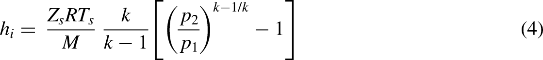
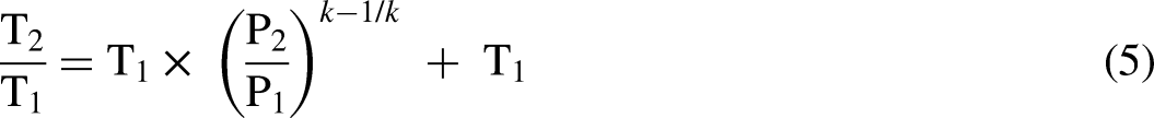
Centrifugal compressors operation is such that, gas flows through the inlet, with increasing velocity, before reaching the diffuser which decreases its velocity, resulting in an increase in pressure and temperature at the outlet. Compressors operate safely within the choke and surge limits and at different speeds. The compressor performance curve helps to limit compressor operation within the safe zone and optimize operation by ensuring it operates at or below its maximum efficiency. The performance curve includes several curves such as head versus efficiency, discharge pressure versus horsepower, and pressure ratio versus efficiency curve, which are useful in determining the operating region of the compressor and the point with minimum cost, where there is a maximum efficiency as shown in Figures 2 and 3. The energy required to compress a gas in an adiabatic process is referred to as the isentropic head, also expressed in meter. The head developed by the compressor is defined as the amount of energy supplied to the gas per unit mass of gas, Tabkhi et al. (2009). For a gas at a certain suction pressure and temperature with specified delivery pressure, the isentropic head is required to meet this delivery pressure, which is also a function of pressure ratio. The isentropic head represents the energy required in a reversible adiabatic compression for an isentropic compression of a perfect gas, the relationship between the isentropic head, temperature and pressure is given by equation (4). To determine the degree of cooling necessary, the discharge temperature is determined from the pressure ratio for an isentropic compression, expressed in equation (5). To define the isentropic compression process for a given gas, suction pressure, suction temperature, and discharge pressures must be known while for polytropic compression, in addition, either the polytropic compression efficiency or the discharge temperature must be known, Hoopes et al. (2019).

h_{i} = \frac{Z_{s} R T_{s}}{M} \frac{k}{k - 1} [{(\frac{p_{2}}{p_{1}})}^{k - 1 / k} - 1]

(4)

\frac{T_{2}}{T_{1}} = T_{1} \times {(\frac{P_{2}}{P_{1}})}^{k - 1 / k} + T_{1}

(5)

Figure 2.

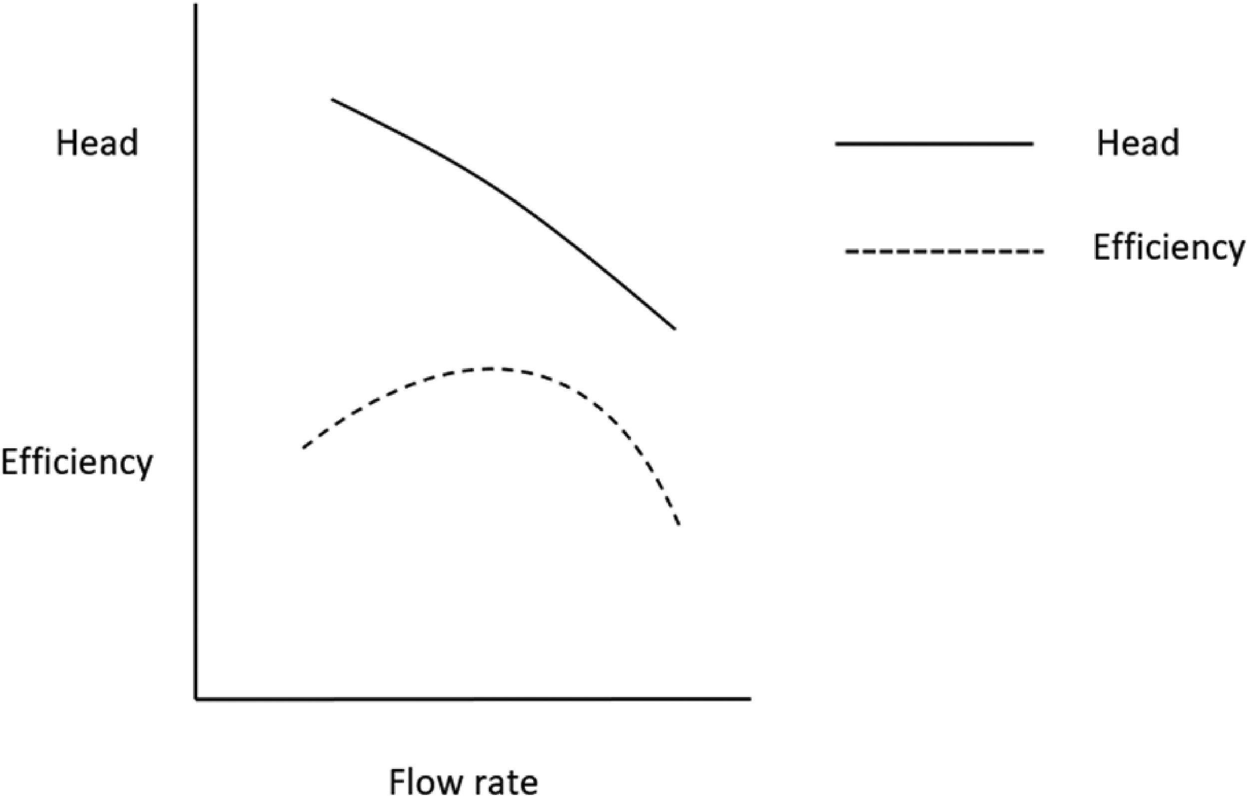
Head, efficiency performance curve, Theodore (2001).

Figure 3.

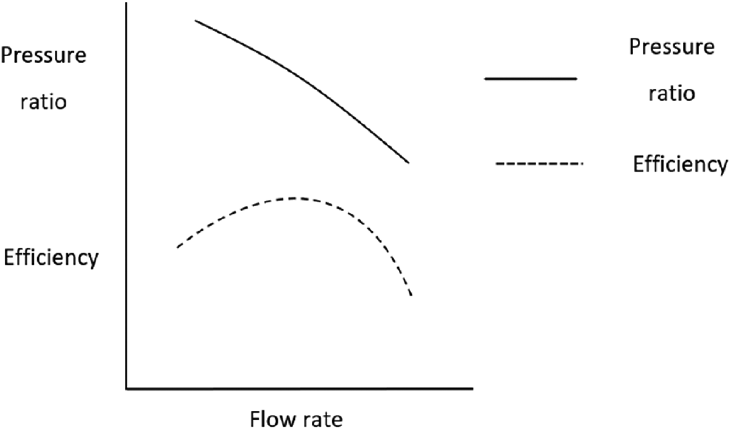
Pressure ratio, efficiency curve, Theodore (2001).

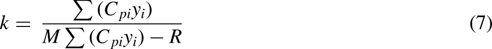
If the driver allows, the speeds of a compressor can be controlled to vary the pressure ratio across and discharge pressure, and the variation of the speed with the flow rate also gives the efficiency, equation (6) and (7) are used in this paper to determine the head and efficiency.

\frac{h_{i}}{ω^{2}} = b_{1} + b_{2} \frac{Q_{s}}{ω} + b_{3} {(\frac{Q_{s}}{ω})}^{2}

(6)

The isentropic exponent is calculated by the heat capacity of the components in gas and their mole ratio using equation (7), while the isotropic efficiency, is shown in equation (8). The mechanical power is expressed in equation (9).

k = \frac{\sum (C_{p i} y_{i})}{M \sum (C_{p i} y_{i}) - R}

(7)

η_{i} = b_{4} + b_{5} \frac{Q_{s}}{ω} + b_{6} {(\frac{Q_{s}}{ω})}^{2}

(8)

P = \frac{1}{η_{m}} \times m_{i}^{\dot{h}} = \frac{\dot{m} h_{i}}{η_{m} η_{s}}

(9)

From power, fuel consumption is derived, by dividing power by the mechanical efficiency, driver efficiency, and lower heating value as shown in equation (10), as shown, fuel consumption increases with compressor speed, gas flow, and head and decreases with increased efficiencies.

m_{f} = \frac{m_{c} h_{i}}{η_{i} η_{m} η_{d} L H V}

(10)

where

h_{i}

is isentropic head,

Z_{s}

is compressibility at the compressor suction, R is gas constant,

T_{s}

is the temperature at the suction,

M

is molecular mass, k is the isentropic exponent,

P_{2}

is the discharge pressure of the compressor,

P_{1}

is the inlet pressure at the compressor suction,

T_{2}

is the discharge temperature of the compressor,

T_{1}

is the inlet temperature,

h_{i}

is the isentropic head,

ω

is the compressor speed,

b_{1}

b_{2}

b_{3}

are the coefficients of the isentropic head,

Q_{s}

is the suction flow rate of the compressor,

C_{p i}

is the heat capacity of the gas component,

y_{i}

is the mole fraction, M is the molecular mass, R is the universal gas constant,

η_{i}

is the isentropic efficiency,

b_{4}

b_{5}

b_{6}

are the coefficients of the isentropic efficiency,

Q_{s}

is the suction flow rate, P is the mechanical power,

η_{m}

is the mechanical efficiency,

\dot{m}

is the mass flow (kg/s),

η_{s}

is the isentropic efficiency,

η_{i}

is the isentropic efficiency,

m_{c}

is gas flow throughput in Compressor,

η_{d}

is the driver efficiency,

L H V

is lower heating value.

Genetic algorithm

Wirsansky (2020) describes GA as a simplified form of Darwinian evolution in nature which is based on:

The principle of variation: The individuals of a specie vary to some extent in attribute.

Inheritance: Some traits are constantly passed from parent to offspring.

Selection: specimens with traits with better adaptation produce more offspring, thereby increasing fitness or adaptation.

According to Wirsansky (2020), GA involves iterations where it examines the Individuals using the fitness function, where the fitness function is the optimization target. The selection process follows the evaluation of the population, selection determines which individual will reproduce to create the next generation, (Wirsansky, 2020). The crossover process follows the selection process, which involves using the parents form the selection operation to create a new individual by interchanging their chromosomes, there are various kinds of crossover operations, (Wirsansky, 2020). The final process is the mutation operation, according to Wirsansky (2020), the operation aims to refresh the population consistently and randomly by introducing new patterns in the chromosomes to search for a solution in unexplored areas of the solution space. Wirsansky (2020) notes the advantages of GA as:

Potential for global optimization: It is less likely to get trapped by a local minimum or maxima due to maintaining a diversity of solutions in every population.

Handles problems without a mathematical description: For instance, problem based on human opinion, or where comparisons determine a better solution

Supports parallel and distributed processing: Individual fitness is determined independently which can also be determined concurrently, furthermore concurrency can be applied to the selection, crossover, and mutation operations.

Suitable for continuous learning: GA can find an optimum solution after environmental changes.

And the disadvantages include:

The need for special definition: It requires the right fitness function, chromosome form, and selection, crossover, and mutation operators.

Hyperparameter tuning: It requires definition for parameters such as population size, mutation rate

Computationally intensive computations: It becomes demanding due to large populations.

The possibility of premature convergence: An individual with a high fitness compared to a population may be duplicated that it becomes the only solution in the population.

No guaranteed solution.

The flow of a GA is shown in Figure 4. To prepare a problem for a GA, the variables are represented by chromosomes, where the value of each gene in the chromosomes is represented by binary, integer, or real numbers. The breeding process which involves exchanging genetic information is emulated by selection operator while random mutation is emulated the crossover operator. A GA maintains a population of individuals, each with a unique chromosome, thus multiple individuals create a pool of chromosomes. At every generation the individuals are assessed by the fitness function, the fitness fiction is used for improving the search process, individuals with higher fitness function are favored during selection to produce the next population, the fitness function also determines the best solution or individual in every population. To ensure that the genes of the best induvial are not lost, the best genes are preserved and passed directly to the next generation. With each new generation, individuals with better fitness are found, this process continues until the last generation.

Figure 4.

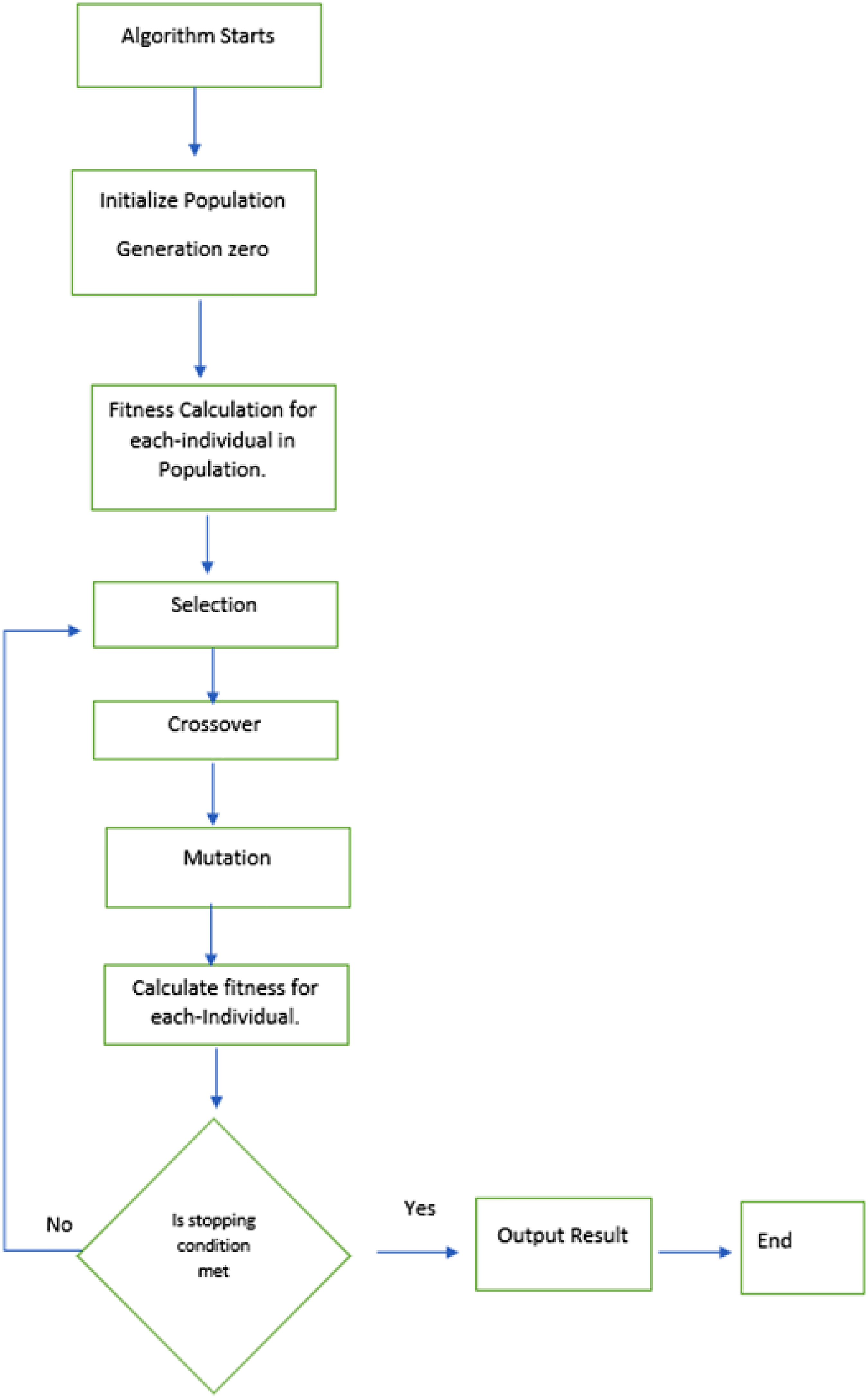
Genetic algorithm, Wirsansky (2020).

After an individual is created, there may be mutation, the mutation operator randomly flips the genes which may accidentally find a better solution, this also makes the GA less alike to a random function. The last step is setting the conditions that stop the algorithm, there are various conditions that can be used. The common conditions are a specified number of generations; the number of improvements over the last few generations, which is set, by storing the best fitness value at every generation, and comparing with the best fitness values from recent generations. GA is a unique optimization method which utilizing the fitness function to find the best solution. The fitness function is consisted of the objective function and constraints. The genes encode the control variables such as gas flow or compressor speed and evolving the population determines a better solution until a global solution is found. GA can also optimize multiple solutions simultaneously (Wirsansky, 2020).

Material and method

Two gas networks were optimized with a GA. The first was a simple network that confirmed that a GA could optimize a gas network. The second network is the main problem with the two compressor stations. The methodology based on a GA was implemented by solving a first gas network (without a compressor station) to determine the optimum flow rates and pressure drops that result in a minimum loop pressure drop summation with a value approximately zero. The equality constraint constrains the flow at every node such that all inflows are equal to all outflows. The equality constraints also ensure all supply flows are equal to the load at the demand point. Solving the network requires estimating the variables for each component in the network, such as the pressure drop for the pipes and the flow rate based on the flow equation, and the Kirchhoff's laws. Before simulation, the gas network is prepared for initial estimation of parameters such as flow and pressure drop, preparation includes identification of the tree and cords, the tree is a pipe which is initially assigned an arbitrary flow with a value greater than zero, while a cord is a pipe assigned with an initial flow of zero. The aim of tagging a pipe as tree or cord is to break the flow continuity within loops in a gas network, such that no loop is composed with only tree pipes. The methodology of this paper involves firstly estimating the initial flow at the trees and assigning zero to the cords. GA creates a variety of solutions with fulfill the mass balance constraint. For the first gas network, the fitness function is the summation pressure drop for every pipe flow in a loop, while for the second gas network, there is modification. The simulation is simplified due to a single gas composition, a single gas supply, constant temperature, and elevation. Challenges in gas network simulation include setting the flow direction, which could be fixed or mutable. Pipes connecting the supply to other pipes have a fixed flow direction due to more significant pressure at the supply point. In contrast, the flow direction at other pipes may change during simulation. A fixed flow direction is required for pipes connecting the supply node to other nodes (pipe 12, 13, and 14 in gas network 1). In contrast, the other pipes (pipe23 and thirty-four in gas network 1) have a mutable direction as shown in Figure 5. For pipes with a mutable direction, the flow directions were generated randomly at the creation of the individual. The flow direction can be represented by the first digit of the chromosome in this case, it was generated using the random function in Java. Another challenge is the mixing rule applied at nodes with multiple incoming pipes to estimate the average parameter value; for node with multiple incoming pipes the average value at the node is the sum of all the pressure of the gas stream flowing into the node divided by the total incoming pipes.

Figure 5.

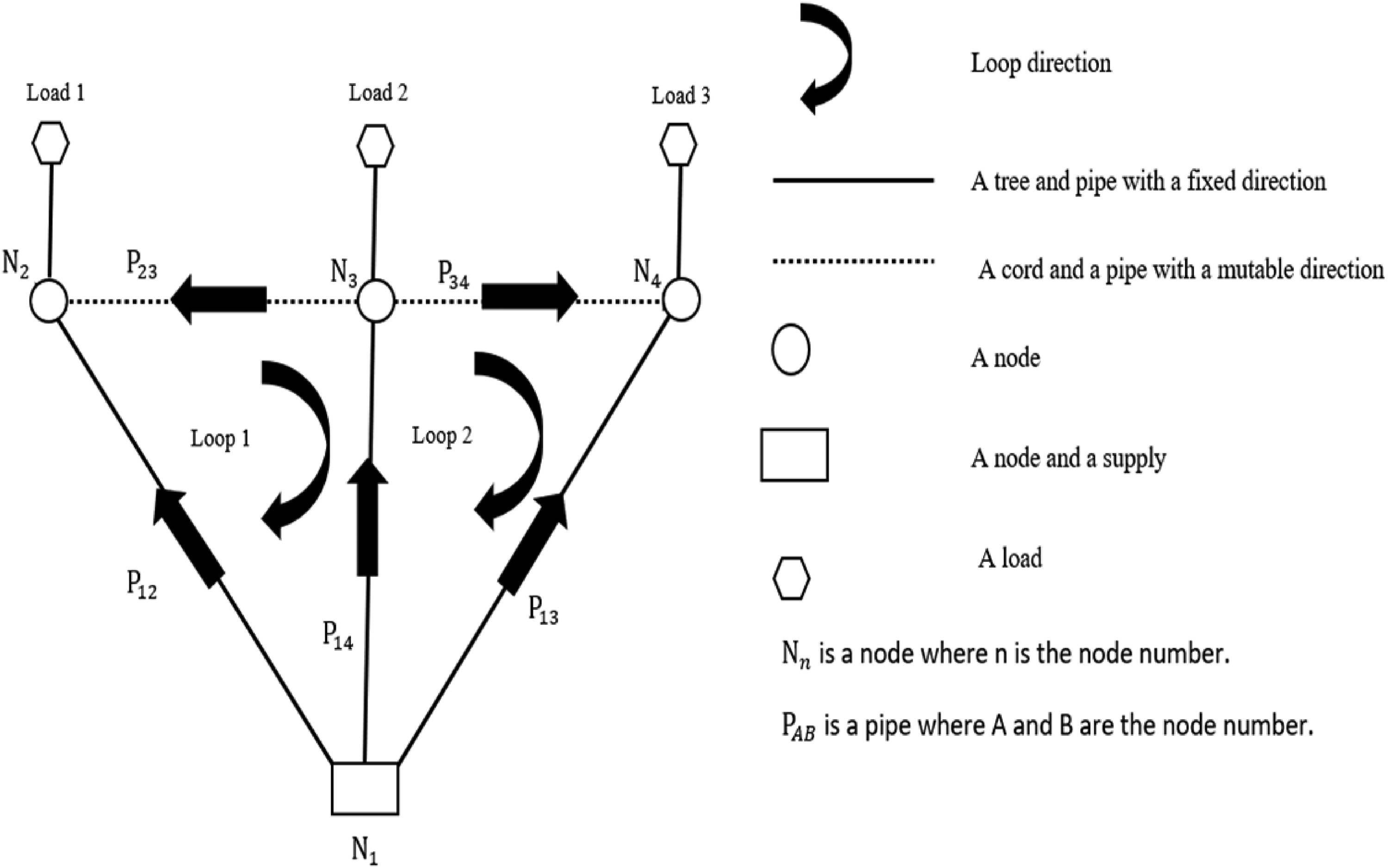
Gas network one, Osiadacz (2001).

Gas network1 preliminary problem

The approach for solving network one with a GA are:

First, create a population of individuals, where an individual contains a unique gas network and gene. For the gas network, for every loop assign the tree and cord, assign a value for flow at the tree and zero at the cord.

From the chromosomes assign a flow for the cord.

At each pipe, determine the pressure drop, and for each loop, determine the sum of pressure drop for every pipe, where the pressure drop is positive if pipe direction is the same as loop direction, otherwise negative.

Evolve the population, except for the best individual at the zero indexes of the population. At the beginning of the algorithm, it recognizes individuals at the zeroth index as the fittest individual. The zeroth index is stores the fittest individual. The fittest individual is compared to every individual in the population until it finds a fitter individual, which replaces the individual at the zeroth index. This process of finding the fittest individual within a population and across generations is called evolution, which involves selection, crossover, and mutation. Evolution creates a new population and attempts to find a better individual with better fitness. The fitness function is the sum of the pressure drop across a loop and its associated constraint, which is the required pressure at the demand; in the case of this network, it is easier to find a solution due to only two loops. Figure 6 shows the flow of the GA, the basic operations involved in making a new population involves selection, crossover, and mutation.

The selection operation involves selecting two fittest individuals to serve as a parent. Selection takes the fittest individual from a temporary population based on an arbitrary size, also known as the tournament size.

The crossover operation involves exchanging the genes of a parent pair to produce a new individual. The algorithm randomly chooses which gene to select from either parent based on the probability value known as the crossover rate.

The mutation operation involves flipping the genes of a chromosome to introduce a new search area in the solution space. Mutation is determined by the mutation rate, and it is usually of a low probability value.

From the new population generated, the fittest individual is identified and is passed to the next generation to preserve the genes of the best individual across generations. The simulation continues until the last generation.

Figure 6.

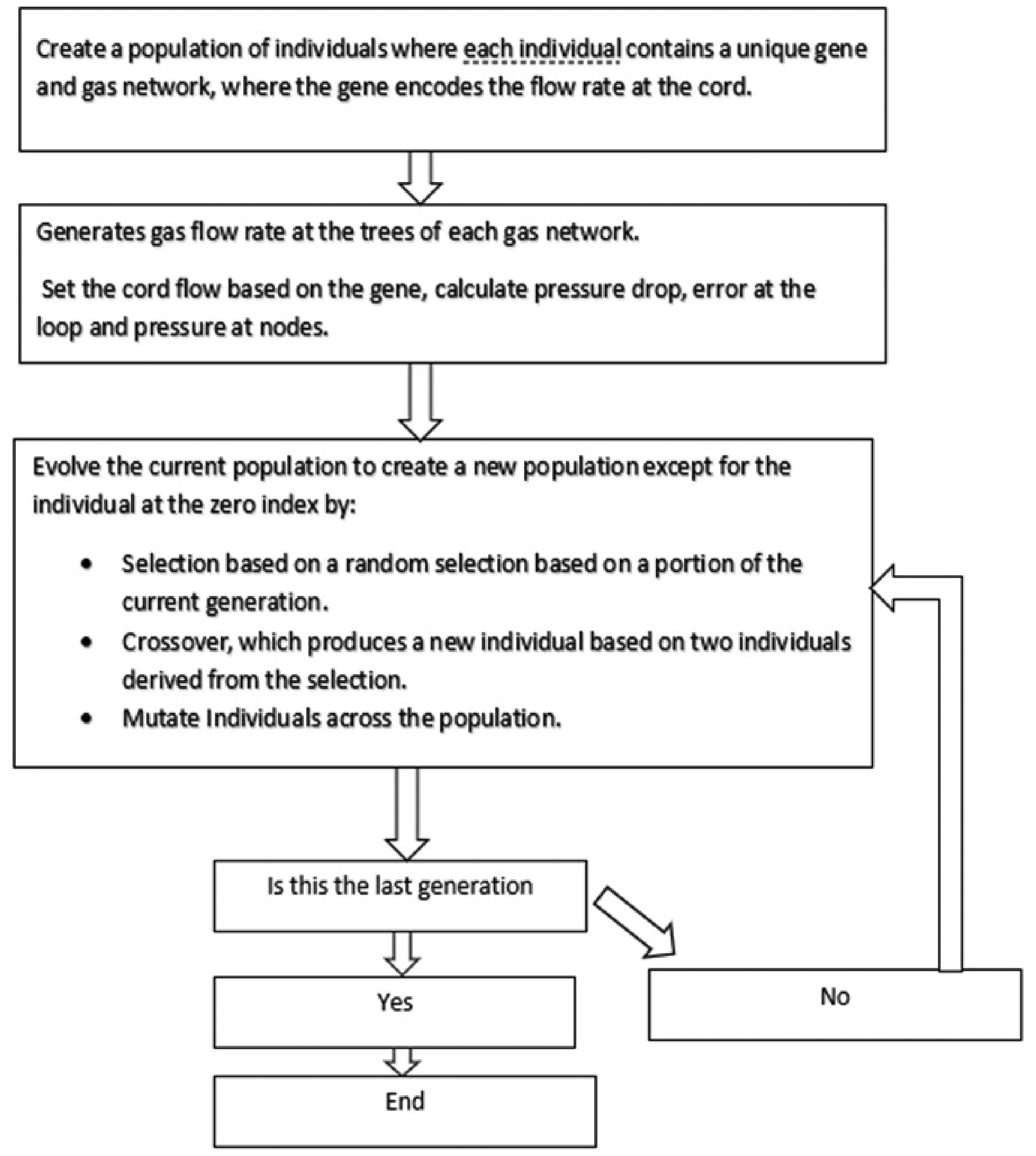
Over all algorithm to solve the gas network.

The first problem is a preliminary problem used to confirm the effectiveness of a GA in solving a gas network problem. The gas network comprises five pipes, one source node, and three demand nodes, as shown in Figure 5. Parameters of the GA include a population size of two hundred, a crossover and mutation rate of 0.9, a tournament size of two hundred, a chromosome length of twelve, and a generation of 1,000. The chromosome encode pipe 23 and 34. The parameters of the gas network are in Table 1, gas is supplied at a rate of 530 m³/h and at a pressure of 30.0 bar.

Table 1.

Parameters for the gas network one network, Osiadacz (2001).

Pipe	Diameter [m]	Length [mm]		Pressure [mbar]	Supply [m³/h]	Demand [m³/h]
12	680	150	Node1 (supply)	30.0	530	0.0
13	500	100	Node2			250.0
14	420	150	Node3			100.0
23	600	100	Node4			180.0
34	340	100

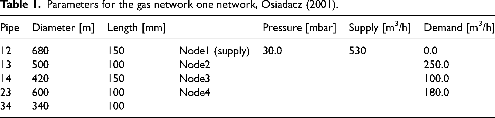
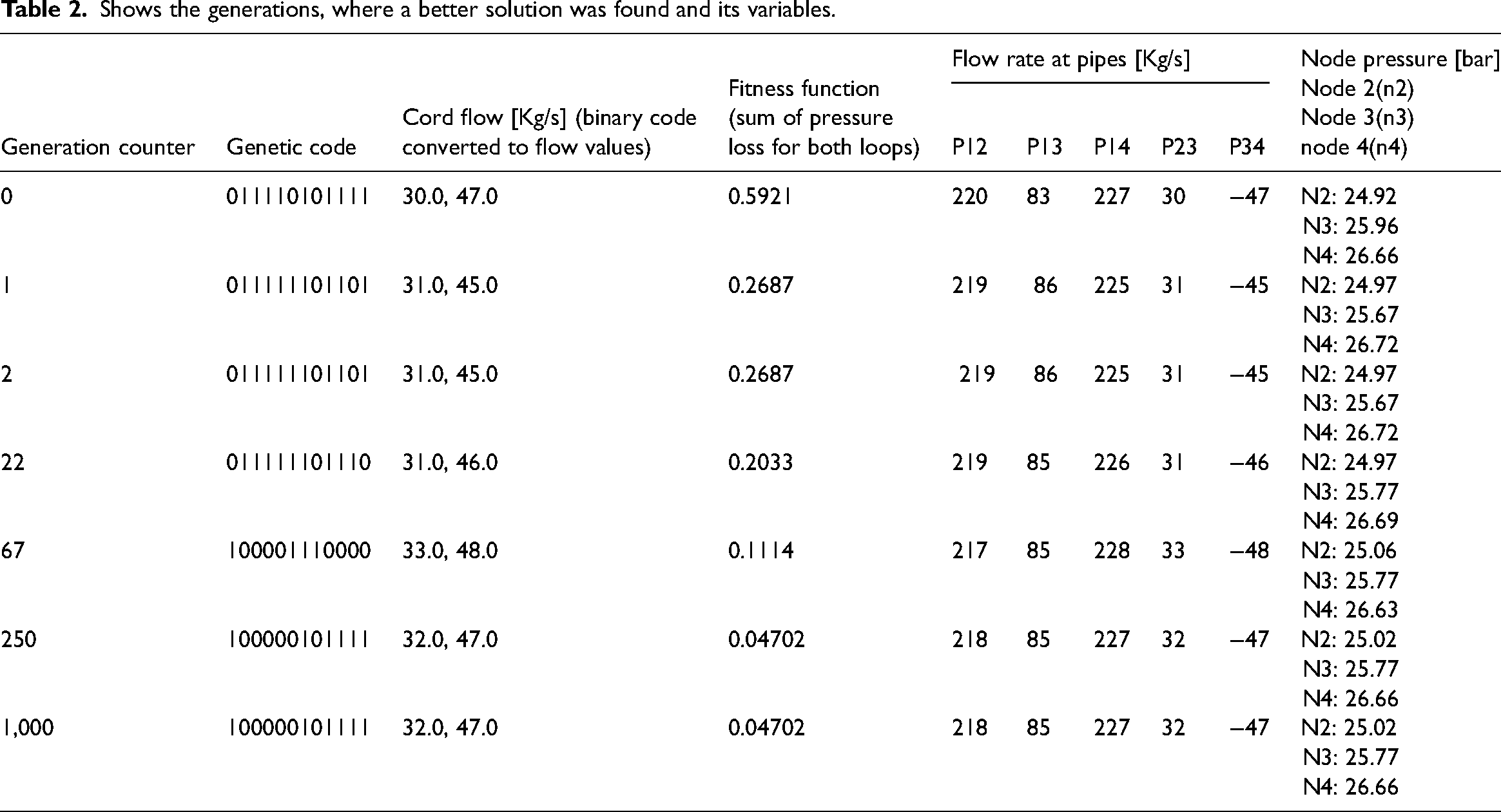
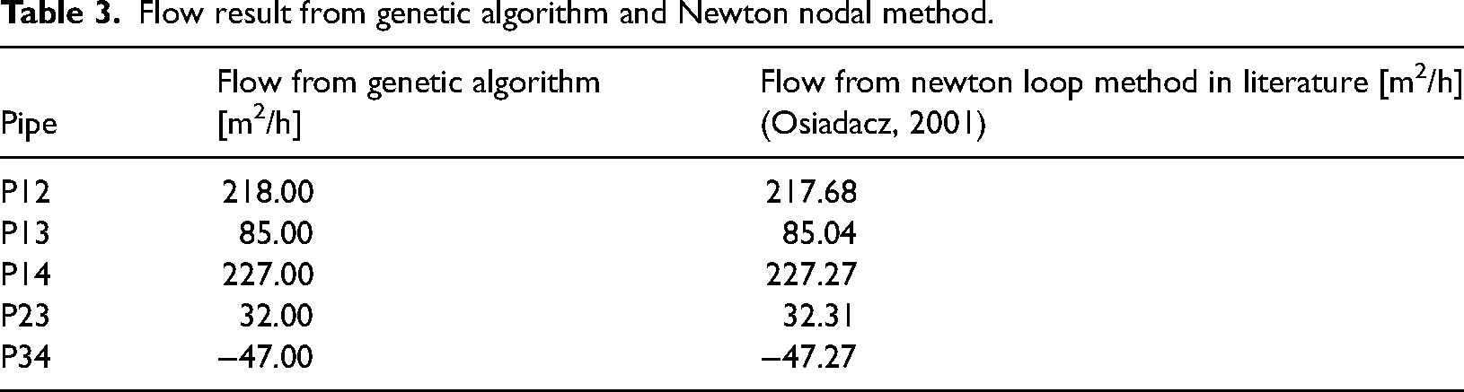
Consumer demand at loads 2, 3, and 4 are 250, 100, and 180 m³/h, respectively. The chromosomes encode gas flow at pipes 23 and 34 as genes. During the simulation, the algorithm printed the best individual for visual comparison. Visual inspection observed the fitness value decreasing, indicating an improvement of the solution for the gas network. Table 2 shows the generations where the GA found a better solution. Comparing result from GA with newton loop method showed a complete match, as shown in Table 3.

Table 2.

Shows the generations, where a better solution was found and its variables.

Generation counter	Genetic code	Cord flow [Kg/s] (binary code converted to flow values)	Fitness function (sum of pressure loss for both loops)	Flow rate at pipes [Kg/s]					Node pressure [bar]Node 2(n2)Node 3(n3)node 4(n4)
Generation counter	Genetic code	Cord flow [Kg/s] (binary code converted to flow values)	Fitness function (sum of pressure loss for both loops)	P12	P13	P14	P23	P34	Node pressure [bar]Node 2(n2)Node 3(n3)node 4(n4)
0	011110101111	30.0, 47.0	0.5921	220	83	227	30	−47	N2: 24.92N3: 25.96N4: 26.66
1	011111101101	31.0, 45.0	0.2687	219	86	225	31	−45	N2: 24.97N3: 25.67N4: 26.72
2	011111101101	31.0, 45.0	0.2687	219	86	225	31	−45	N2: 24.97N3: 25.67N4: 26.72
22	011111101110	31.0, 46.0	0.2033	219	85	226	31	−46	N2: 24.97N3: 25.77N4: 26.69
67	100001110000	33.0, 48.0	0.1114	217	85	228	33	−48	N2: 25.06N3: 25.77N4: 26.63
250	100000101111	32.0, 47.0	0.04702	218	85	227	32	−47	N2: 25.02N3: 25.77N4: 26.66
1,000	100000101111	32.0, 47.0	0.04702	218	85	227	32	−47	N2: 25.02N3: 25.77N4: 26.66

Table 3.

Flow result from genetic algorithm and Newton nodal method.

Pipe	Flow from genetic algorithm [m²/h]	Flow from newton loop method in literature [m²/h] (Osiadacz, 2001)
P12	218.00	217.68
P13	85.00	85.04
P14	227.00	227.27
P23	32.00	32.31
P34	−47.00	−47.27

Main gas network problem

The data for gas network two are obtained from Tabkhi (2007) thesis titled “Optimization de Réseaux de Transport de Gaz”. The gas network comprises of one supply and delivery node, fifteen pipes, eighteen interconnecting nodes, two compressor stations, and six compressors, as shown in Figure 7. The supply node emulates gas supply at a fixed pressure with a limit of 2%, while the delivery node emulates supply at the demand point for consumption. Optimization involves determining the set of gas flow at pipes G3, G4, G5, G9, G10, and G11 and compressor speed at compressors C1, C2, C3, C4, C5, and C6. Optimization consists of two main simulations: flow and speed optimization, respectively. In the first simulation referred as the flow optimization, the algorithm optimizes flow by varying the flow due to varying the chromosomes; the chromosomes encode flow at G3, G5, G9, and G11. The flows derived from the chromosomes are subtracted from the tree flow at pipe G4 and G10 to determine the flows at G4 and G10. This approach of encoding some flows helps preserve the node's material balance. The fitness function is the summation of the minimum pressure loss at every loop of the compressor station. The flow from flow optimization will serve as an input in the second optimization while remaining constant. In speed optimization, the algorithm encodes the speed in the chromosomes and optimizes the speed according to the fitness function, which is the minimum fuel consumption. The objective function is the minimum fuel consumption at each compressor station, which is a function of the head across each compressor, its speed, and gas flow into the compressors. The compressor speed controls the rate of fuel consumption, more speed results in more compression and fuel consumption. The solution involves finding the combination of six speeds that result in the minimum fuel consumption. The chromosomes encoded six speeds in this research and GA search for the speed combination that results in minimum fuel consumption.

Figure 7.

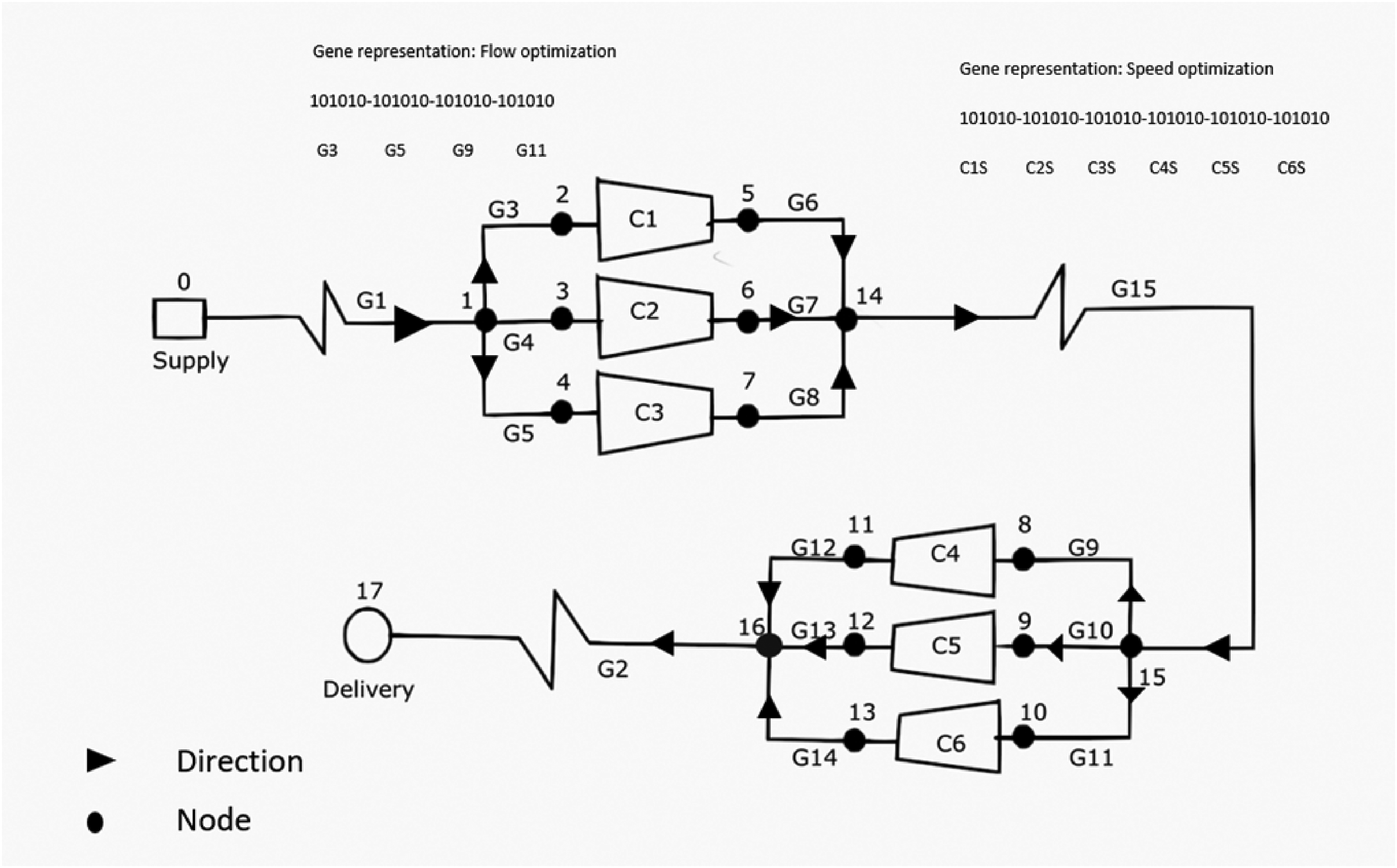
Gas network two.

The optimization is divided into two main optimizations as follows:

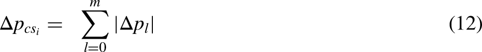
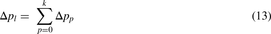
First, flow optimization encodes flows as genes with predetermined flow directions (Figure 7) and a fixed compressor speed at 166.7 rpm (revolutions per minute). The algorithm simulates each compressor station as two loops. Optimizing the loops determines the flows at the outlet of nodes 1 and 15, which have three outgoing pipes. Here the fitness function sums the absolute pressure drops for both compressor stations. For each station and every loop within, the summation considers the numeric sign resulting from the summation of the loop pressure drops. The fitness function is given by equations (11) to (13).

Secondly, Speed optimization uses the flows from flow optimization, where flow is fixed, and speed is varied. Speed optimization searches for the set of speeds that gives the minimum fuel consumption considering both compressor stations, constrained by the pressure required at the demand node and the speed limit. In this optimization, the fitness function combines the objective and demand constraints.

The algorithm assigns a loop direction to each loop, and the pipe direction corresponds to the predetermined directions. During simulation, every pipe with the same direction as the loop would have a positive pressure loss and a negative pressure drop for pipes with an opposite direction. The simulation is simplified since direction switch in gas flow is not considered. Optimizing the flows across each loop helps determine the flows for multiple pipes coming out of a single node such as node1 and fifteen. The algorithm generates flows for two pipes taking flows from node 1, and both pipes are in different loops, where each loop gives a summation of pressure drop for every pipe it contains. Summation should be zero or close to zero. A GA uses a fitness function for comparisons to determine the best individual or solution. In this simulation, the fitness function is the summation of the pressure drop for both compressor stations in absolute value. Each compressor station sums up all the pressure drops for every loop, considering the numeric signs, and for every loop, the summation considers the numeric signs of the pressure loss of each pipe as shown in equations (11)–(13).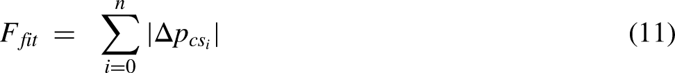

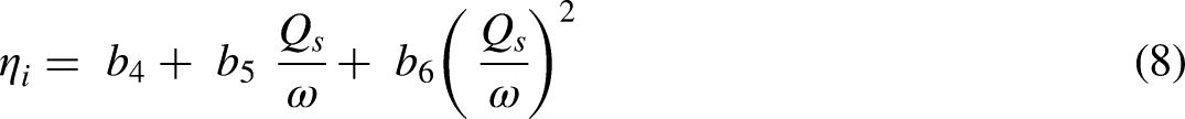
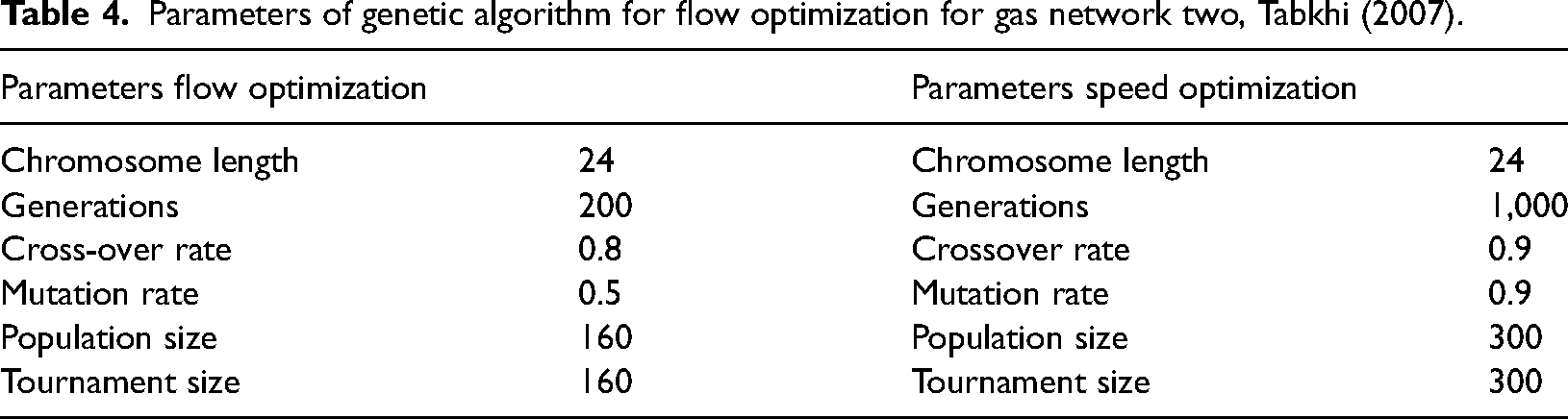
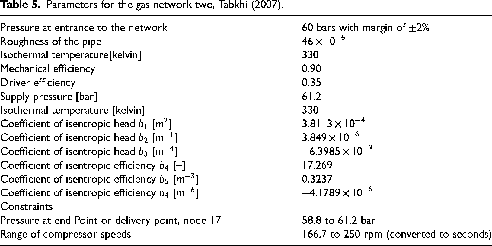
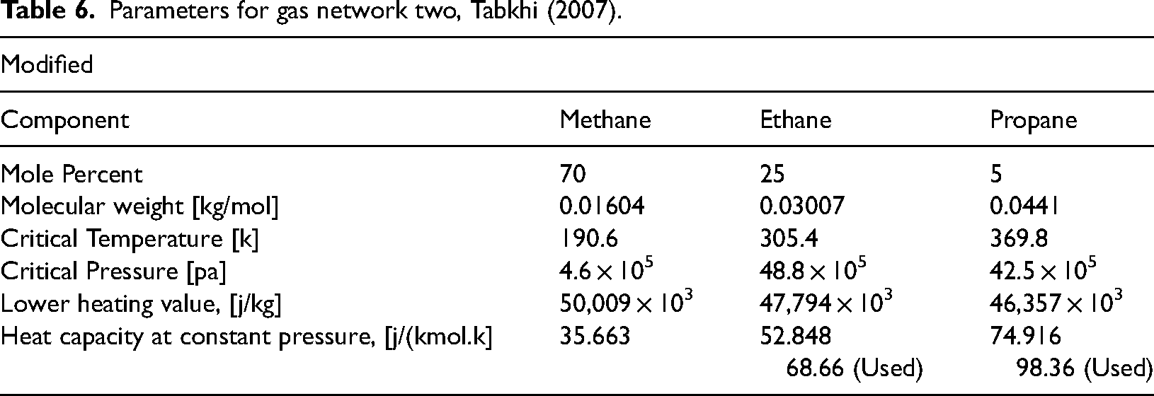
F_{f i t} = \sum_{i = 0}^{n} | Δ p_{c s_{i}} |

(11)

Δ p_{c s_{i}} = \sum_{l = 0}^{m} | Δ p_{l} |

(12)

Δ p_{l} = \sum_{p = 0}^{k} Δ p_{p}

(13)

where

F_{f i t}

—Fitness function for flow optimization; i—compressor station count; n—total number of compressors;

| Δ p_{c s_{i}} |

—total pressure loss for each compressor station in absolute; l—loop count; m—total number of loops;

| Δ p_{l} |

—total pressure loss for each loop in absolute; p—pipe count; k—total pipe;

Δ p_{l}

—total pressure loss for each loop;

Δ p_{p}

—pressure loss for each pipe.

The GA was written in the Java programing language. The algorithms consist of the class templates for GA, population and individual, compressors, compressor-station, gas network, loop, pipe, and node. In the first optimization, the algorithm encodes the flows as chromosomes, while for the second optimization, the algorithm encodes six compressors speed as chromosomes. The class representing the population creates an object composed of an arbitrary number of individuals. Every individual contains a unique gas network with a unique gene encoding flow for pressure loss minimization and speeds for fuel consumption minimization. The GA contains the function evolve, which evolves the population by calling other functions for selecting fit parents for crossover operation to produce a new individual and for random mutation. Across generations, the gene of the best individual is passed to the next population, ensuring the preservation of the fittest individuals across generations which improves the solution. For flow optimization, the GA narrows the search areas by considering one compressor station for half of the generation and the other station for the other half of the generation. The chromosome has a length of twenty-four binary digits. Each compressor station makes up half of the chromosome, and two pipes in the compressor station make up half of the chromosome. Each flow is a six-digit binary unit, where the maximum and minimum values of a six-digit binary unit are 63 and 0, respectively. The GA optimizes only flow in the flow optimization. The aim is to determine the optimum flow from searching through the different combinations that conform with Kirchhoff's second law that pressure loss across the loop should be close to zero. For flow optimization, the parameters for the GA are Gene length of twenty-four; a generation of two hundred; crossover rate of 0.8; mutation rate of 0.5; population size of 160; tournament size of 160. The parameters of GA are given in Table 4, and that of gas network two are in Tables 5 and 6. It is assumed that the coefficient of the isentropic head and efficiency are the same for every compressor, this means that the isentropic efficiency for every compressor will be determined by the same coefficients, given previously by equation (8).

Table 4.

Parameters of genetic algorithm for flow optimization for gas network two, Tabkhi (2007).

Parameters flow optimization		Parameters speed optimization
Chromosome length	24	Chromosome length	24
Generations	200	Generations	1,000
Cross-over rate	0.8	Crossover rate	0.9
Mutation rate	0.5	Mutation rate	0.9
Population size	160	Population size	300
Tournament size	160	Tournament size	300

Table 5.

Parameters for the gas network two, Tabkhi (2007).

Pressure at entrance to the network	60 bars with margin of ±2%
Roughness of the pipe	46 × 10⁻⁶
Isothermal temperature[kelvin]	330
Mechanical efficiency	0.90
Driver efficiency	0.35
Supply pressure [bar]	61.2
Isothermal temperature [kelvin]	330
Coefficient of isentropic head $b_{1}$ [ $m^{2}$ ]	3.8113 × 10⁻⁴
Coefficient of isentropic head $b_{2}$ [ $m^{- 1}$ ]	3.849 × 10⁻⁶
Coefficient of isentropic head $b_{3}$ [ $m^{- 4}$ ]	−6.3985 × 10⁻⁹
Coefficient of isentropic efficiency $b_{4}$ [–]	17.269
Coefficient of isentropic efficiency $b_{5}$ [ $m^{- 3}$ ]	0.3237
Coefficient of isentropic efficiency $b_{4}$ [ $m^{- 6}$ ]	−4.1789 × 10⁻⁶
Constraints
Pressure at end Point or delivery point, node 17	58.8 to 61.2 bar
Range of compressor speeds	166.7 to 250 rpm (converted to seconds)

Table 6.

Parameters for gas network two, Tabkhi (2007).

Modified
Component	Methane	Ethane	Propane
Mole Percent	70	25	5
Molecular weight [kg/mol]	0.01604	0.03007	0.0441
Critical Temperature [k]	190.6	305.4	369.8
Critical Pressure [pa]	4.6 × 10⁵	48.8 × 10⁵	42.5 × 10⁵
Lower heating value, [j/kg]	50,009 × 10³	47,794 × 10³	46,357 × 10³
Heat capacity at constant pressure, [j/(kmol.k]	35.663	52.84868.66 (Used)	74.91698.36 (Used)

Result and discussion

The first gas network (gas network 1) in Figure 5 was used as a preliminary problem to determine whether GA can solve a simple gas network with five pipes, one source (supply), and three nodes. The simulation used one thousand generations, and for each generation, a population size of two hundred individuals. The fitness function is a summation of the pressure loss for both loops in the network. The result in Table 2 showed that the chromosomes change from 011110101111 to 100000101111 from the first to the last generation, respectively. The objective function (Summation of loop error for all loop) was also reduced from 0.5921 to 0.04702 from the first to the last generation, respectively, which indicated that the error in the loop had reduced significantly, resulting in a more accurate solution. The gas flow for the pipes and the pressure at the nodes of the last generation closely match the result obtained from the newton loop method and literature, as shown in Table 3. The outcome agrees with result of Djebedjian et al. (2008) study, in which GA optimized the design of a gas network by optimizing the pipe diameters, likewise, GA optimize gas network two using the gas flow.

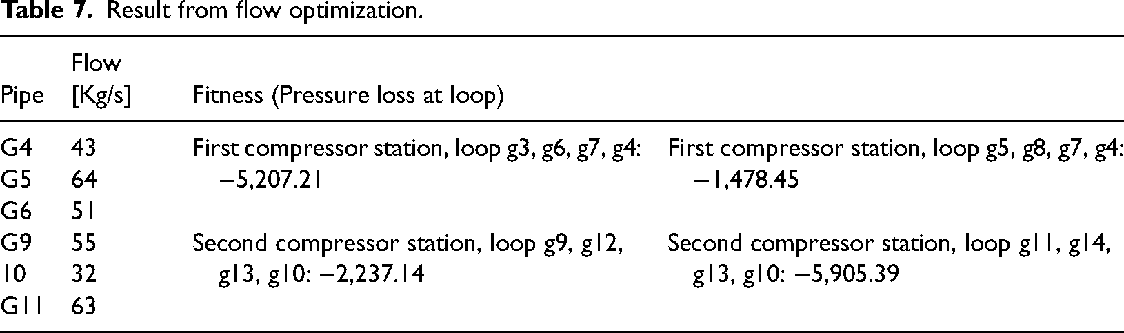
For the main problems (Figure 7, gas network 2), the simulation consists of two parts, first optimizing the flow in the pipes while the speed of all compressors was fixed and of the same value. Secondly, the speed optimization where the optimized flow was fixed, and the speed were optimized. The parameters of GA for the flow and speed optimization are given in Table 4, other parameters for the pipes and gas are given Tables 5 and 6. The result from the flow optimization at the final generation count showed that the first compressor station has a loop error of −5,207.21 and −1,478.45. In contrast, the second has −2,237.14 and −5,905.39, respectively, which suggest that the fitness function, which is the summation of pressure for each loop in the compressor station, is not optimized. It also confirms that compressors break the continuity in a loop, and therefore the pressure losses within a loop cannot be zero.

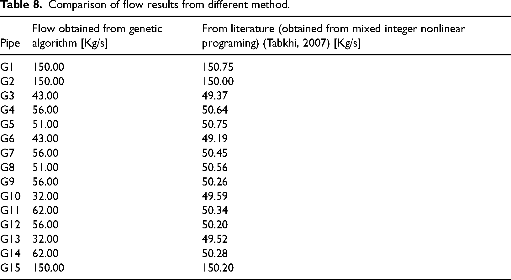
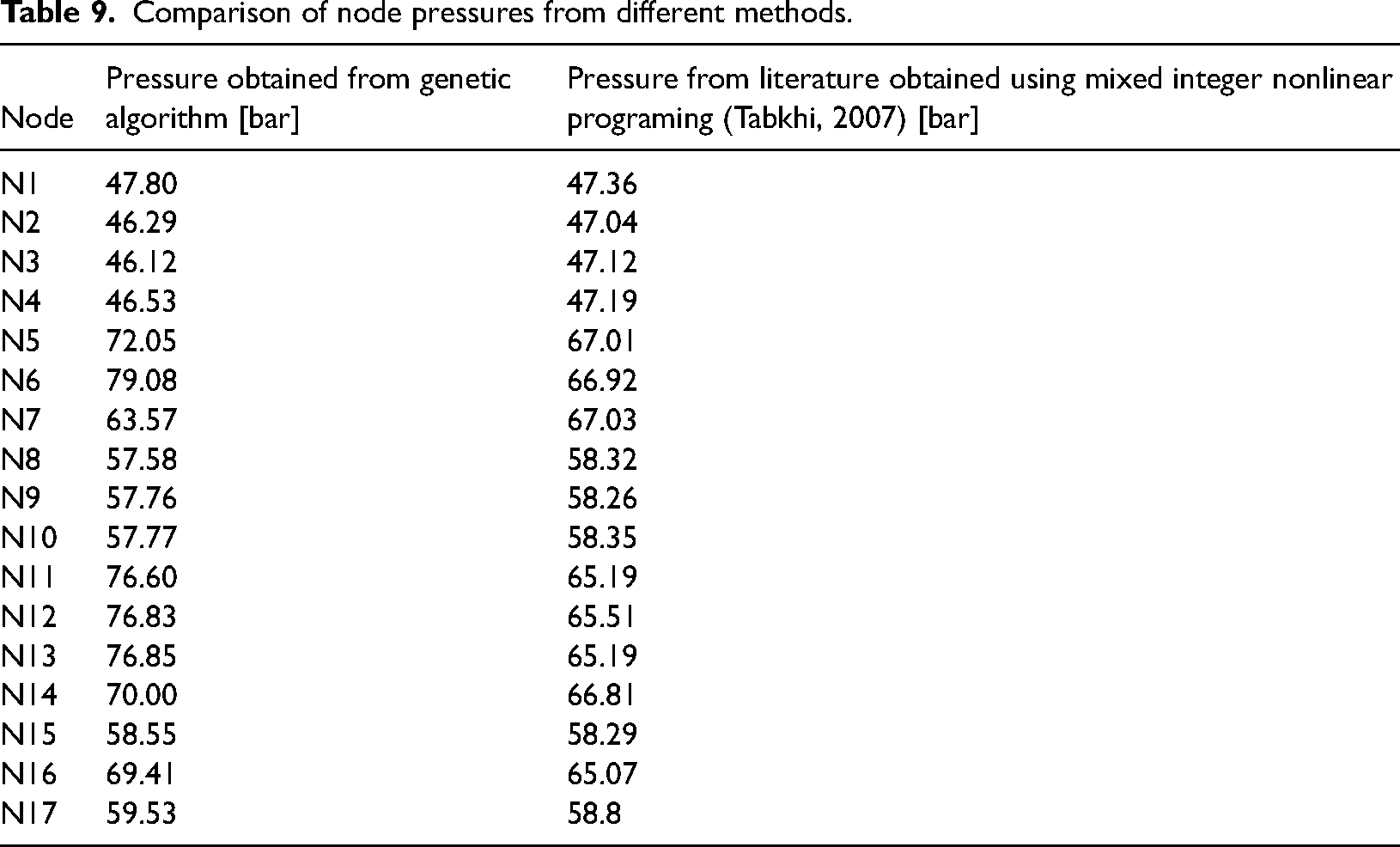
The fitness values are presented in Table 7. The flow optimization results compared with results from literature by Tabkhi (2007) showed that some gas flows are similar in values in pipe G3, G4, G5, G6, and G8 and significantly different values for pipe G10, G11, G13, and G14. Therefore, there is a need to redefine the fitness function which is summation of pressure loss for loops within a compressor station. The result of the flow optimization with the flow from MINLP is in Table 8. From the speed optimization, the optimum node pressures are in Table 9, which also contains the result obtained from MINLP programing. A comparison shows some pronounced differences at the compressor discharge, such as the outlet nodes of 5, 6, 7, 11, 12, and 13. In contrast, the pressure at the inlet nodes before every compressor had a similar value at nodes 2, 3, 4, 8, 9, and 10. Furthermore, the pressure at the demand of 59.53 bar stayed within the required range between 58.8 and 61.2 bar. Therefore, the optimization converged to a solution, although there are significant differences with the result in the literature.

Table 7.

Result from flow optimization.

Pipe	Flow [Kg/s]	Fitness (Pressure loss at loop)
G4	43	First compressor station, loop g3, g6, g7, g4: −5,207.21	First compressor station, loop g5, g8, g7, g4: −1,478.45
G5	64
G6	51
G9	55	Second compressor station, loop g9, g12, g13, g10: −2,237.14	Second compressor station, loop g11, g14, g13, g10: −5,905.39
10	32
G11	63

Table 8.

Comparison of flow results from different method.

Pipe	Flow obtained from genetic algorithm [Kg/s]	From literature (obtained from mixed integer nonlinear programing) (Tabkhi, 2007) [Kg/s]
G1	150.00	150.75
G2	150.00	150.00
G3	43.00	49.37
G4	56.00	50.64
G5	51.00	50.75
G6	43.00	49.19
G7	56.00	50.45
G8	51.00	50.56
G9	56.00	50.26
G10	32.00	49.59
G11	62.00	50.34
G12	56.00	50.20
G13	32.00	49.52
G14	62.00	50.28
G15	150.00	150.20

Table 9.

Comparison of node pressures from different methods.

Node	Pressure obtained from genetic algorithm [bar]	Pressure from literature obtained using mixed integer nonlinear programing (Tabkhi, 2007) [bar]
N1	47.80	47.36
N2	46.29	47.04
N3	46.12	47.12
N4	46.53	47.19
N5	72.05	67.01
N6	79.08	66.92
N7	63.57	67.03
N8	57.58	58.32
N9	57.76	58.26
N10	57.77	58.35
N11	76.60	65.19
N12	76.83	65.51
N13	76.85	65.19
N14	70.00	66.81
N15	58.55	58.29
N16	69.41	65.07
N17	59.53	58.8

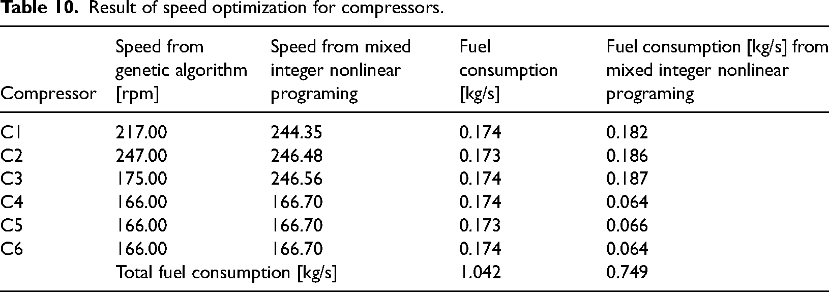
Speed optimization also determines the set of compressor speeds that results in the minimum fuel consumption constrained by pressure at the demand, and the results are in Table 10. Comparisons with the result from MINLP showed similar values in compressors C2, C4 C5, and C6 with significant dissimilarity at compressor C1 and C3.The total fuel consumption for all compressor stations in the gas network is 1.042 kg/s, while the value obtained by Tabkhi (2007) is 0.749 kg/s. Indicating that the MINLP was better at minimizing the fuel consumption, the presence of compressors in a loop means the summation of pressure loss for a loop would not be zero. There is a need for another objective function for flow optimization to obtain more optimized gas flow. A better fitness function should be developed based on the fuel consumption minimization and the pressure constraint at the demand.

Table 10.

Result of speed optimization for compressors.

Compressor	Speed from genetic algorithm [rpm]	Speed from mixed integer nonlinear programing	Fuel consumption [kg/s]	Fuel consumption [kg/s] from mixed integer nonlinear programing
C1	217.00	244.35	0.174	0.182
C2	247.00	246.48	0.173	0.186
C3	175.00	246.56	0.174	0.187
C4	166.00	166.70	0.174	0.064
C5	166.00	166.70	0.173	0.066
C6	166.00	166.70	0.174	0.064
	Total fuel consumption [kg/s]		1.042	0.749

Comparisons with previous studies show the following:

Agreement with results of Elshiekh (2015) which involved optimization of two compressor station with GA to obtain the optimal speeds of all six active compressors simultaneously, and consequently to obtain the minimum fuel-consumption rate subject compressor constraints. Similarly, from the optimization using GA on gas network two, the compressor speeds and fuel consumption were optimized, but the gas flow requires an improved algorithm.

The outcome from gas network two optimization partially agrees with the study of Habibvand and Behbahani (2012). In the study, GA was applied on a transmission line with a compressor station to minimize fuel consumption, bounded by a specified set pressure at next station. The control variables include the mass flow split amongst the compressor units, the compressor performance limitations, the on/off status of each compressor and the aerial cooler pressure drop and temperature. The study shows that compressor speed, the flow split, and the compressor status can be used to optimize the fuel consumption, while from the outcome in gas network two, there is inadequate flow distribution.

The outcome of gas network two optimization also agrees with the study by Zhang and Wu (2015), which considered both binary and real coding chromosomes with the aim of comparing both the feasibility and the performances of different GA. The outcome showed that real-coded GA yields better solution, which agrees with the outcome from as network two, which shows that binary coding also optimizes compressor station operation.

The results of the optimization of as network two agrees with Zhang and Liu (2017) study which used an IGA to optimize a city natural gas pipeline network shows that the IGA has better applicability in the optimal operation of natural gas pipeline network. In gas network two optimization, using the summation of the pressure drops in the compressor station loop as the fitness function resulted in poor flow distribution and requires improvement.

The outcome of the study from gas network two agrees with the outcome from Li et al. (2011) study, which optimized a gas network with gas supply, purchase cost of gas supply, several delivery nodes, the prize of gas sale to the consumer. Whose outcome shows that GA found the optimum solution which increases the profit, by reducing the quantity of gas going to point with lower sale prize and increasing the quantity going to points with greater sale prize.

Conclusion

GA was first used to optimize gas network one as a preliminary investigation. Gas network one, contains pipes and nodes with three demand nodes. The results converged to a solution and matched values from literature by Osiadacz (2001). The fitness function is the summation of the pressure loss for every loop in the gas network. The outcome agrees with the study by Djebedjian et al. (2008) where pipe diameter was used to optimize the design of a gas network. From the outcome of gas network one, GA was able to optimize the flow distribution for loops without compressors.

GA was also used to solve gas network two, which is the main optimization problem. Gas network two, includes two compressor stations, each with three compressors. The simulation comprises two main parts: flow optimization and speed optimization. For flow optimization, the objective function is the summation of the pressure drop across the loops in a compressor station. In the speed optimization, the objective function was the fuel consumption minimization subject to the pressure required at the demand. The results were compared with literature by Tabkhi (2007), where MNLP solved the same network. From comparisons there were similarities in the pipes’ gas flow, such as in pipe G3, G4, G5, G6, and G8, and significantly different values for pipe G10, G11, G13, and G14. There were also similarities in the pressure at the nodes 2, 3, 4, 8, 9, and 10 but dissimilarities in nodes 5, 6, 7, 11, 12, and 13. Also, there were similarities in the compressor speed at compressor C2, C4 C5, and c6 and dissimilarities at compressor C1 and C3. Although the values were not consistent for the gas flow and node pressure, the pressure at the consumer point (demand) converged within the expected range, which indicates a solution.

The total fuel consumption for all compressor stations in gas network two is 1.042 kg/s, while the value obtained by Tabkhi (2007) is 0.749 kg/s. Indicating that the MINLP was better at minimizing the fuel consumption. The presence of compressors in a loop means the summation of pressure loss for a loop would not be zero and it resulted in inadequate flow distribution, therefore the fitness function to determine flow should be studied for a better representation. The results from the optimization of Gas network two, agrees with other study that compressor speed is useful for fuel consumption minimization such studies include by Elshiekh (2015, by Zhang and Wu (2015), Zhang and Liu (2017), from Li et al. (2011). And disagrees partially with the study of Habibvand and Behbahani (2012) because the summation of pressure drop for each compressor station loop is unsuitable to find the optimum flow flit among the compressor inlets.

Policy recommendation

Based on the findings of using GA to optimize gas network one to determine its node pressure and pipe flow and to optimize a gas network two simultaneously with its compressor station operations, GA should be improved by weighting the pipes to determine the importance of each pipe in the optimization to narrow the search space. Also recommended to borrow concepts from neural network to improve the ability to search for feasible solutions. Furthermore, an improved fitness function is required to determine better gas flow distribution. More innovation should be encouraged by providing more access to data from industries on their operations that emits CO2 and other activities that results in environmental degradation. Access to information on Gas network operations and compressor manufacturer data would encourage researchers to innovate industrial operations.

Data availability

Datasets related to this article can be found at https://data.mendeley.com/datasets/pby229kpgr/1, an open-source online data repository hosted at Mendeley Data (Takerhi, 2022a).

Datasets related to this article can be found through the shared link at https://data.mendeley.com/datasets/g7nb7b9ys7/2, an open-source online data repository hosted at Mendeley Data (Takerhi, 2022b).

Datasets related to this article can be found through the shared link at https://data.mendeley.com/datasets/6zth8gytm4/2, an open-source online data repository hosted at Mendeley Data (Takerhi, 2022c).

Footnotes

Declaration of conflicting interests

The author(s) declared no potential conflicts of interest with respect to the research, authorship, and/or publication of this article.

Funding

The author(s) received no financial support for the research, authorship, and/or publication of this article.

ORCID iD

Matthew Efe Takerhi

References

Adebayo

(2022) Environmental consequences of fossil fuel in Spain amidst renewable energy consumption: A new insight from the wavelet-based Granger causality approach. The International Journal of Sustainable Development and World Ecology. DOI: 10.1080/13504509.2022.2054877.

Adebayo

Agyekum

Kamel

, et al. (2022a) Drivers of environmental degradation in Turkey: Designing an SDG framework through advanced quantile approaches. Energy Reports 8: 2008–2021.

Adebayo

Oladipupo

Kirikkaleli

, et al. (2022b) Asymmetric nexus between technological innovation and environmental degradation in Sweden: An aggregated and disaggregated analysis. Environmental Science and Pollution Research 29: 36547–36564.

Allison

Singh

Thorp

(2019) Upstream compression applications. In: Klaus Brun, and Rainer Kurz (eds.) Compression Machinery for Oil and Gas. Pennsylvania: Gulf Professional Publishing, pp.375–384.

Awosusi

Adebayo

Kirikkaledi

, et al. (2022) Role of technological innovation and globalization in BRICS economies: Policy towards environmental sustainability. The International Journal of Sustainable Development and World Ecology. DOI: 10.1080/13504509.2022.2059032

Dandy

Simpson

Murphy

(1996) An improved genetic algorithm for pipe network optimization. Water Resources Research 32(2): 449–458.

Djebedjian

Shahin

El-Naggar

(2008) Gas distribution network optimization by genetic algorithm, Ninth International Congress of Fluid Dynamics and Propulsion. Alexandria, Egypt: The American Society of Mechanical Engineers, pp. 290–309.

DNV GL (2017) Oil and gas forecast to 2050. Energy transition outlook 2017. Available at: https://www.ourenergypolicy.org/wp-content/uploads/2017/09/DNV-GL_Energy-Transistion-Outlook-2017_oil-gas_lowres-single_3108_3.pdf (accessed 9 January 2022).

Eiger

Shamir

Ben-tal

(1994) Optimal design of water distribution networks. Water Resources Research 30(9): 2367–2646.

10.

Ekhtiari

Dassios

Liu

, et al. (2019) A novel approach to model a gas network. Applied Sciences. DOI:10.3390/app9061047.

11.

El-Mahdy

OFM

Ahmed

MEH

Metwalli

(2010) Computer aided optimization of natural gas pipe networks using genetic algorithm. Applied Soft Computing 10(2010): 1141–1150.

12.

Elshiekh

(2015) Optimization of fuel consumption in compressor stations. Society of Petroleum Engineers 4(1): 59–65.

13.

Fareed

Salem

Pata

, et al. (2021) Role of export diversification and renewable energy on the load capacity factor in Indonesia. Frontiers in Environmental Science 3(5): 23–56.

14.

Habibvand

Behbahani

(2012) Using genetic algorithm for fuel consumption optimization of a natural gas transmission compressor station. International Journal of Computer Applications 43(1): 1–6.

15.

Haddad

Behbahani

Shishesaz

(2013) Power consumption minimization of Khormoj compressor station. Iranian Journal of Oil & Gas Science and Technology 3(2): 66–79.

16.

Hoopes

Alison

Kurz

(2019) Oil and gas compressor basics. In: Klaus Brun, and Rainer Kurz (eds.) Oil and Gas Compressor Basics. Pennsylvania: Gulf Professional Publishing, pp.3–4.

17.

Jia

Yang

, et al. (2011) Adaptive genetic algorithm for steady-state operation optimization in natural gas networks. Journal of Software 6(3): 452–459.

18.

Mohring

Hoffman

Halfman

, et al. (2003) Automated Model Reduction of Complex Gas Pipeline Networks. Houston Texas: Pipeline Simulation Interest Group.

19.

Narváez

P-C

Galeano

(2004) Genetic algorithms for the optimization of pipeline systems for liquid distribution (2). Ciencia, Tecnología & Futuro 2(5): 117–130.

20.

Osiadacz

(2001) Steady state simulation of gas networks. Warsaw: Fluid Systems.

21.

Osiadacz

Isoli

(2020) Multi-objective optimization of gas pipeline networks. Energies. DOI:10.3390/en13195141.

22.

Singh

Nain

PKS

(2012) Optimization of natural gas pipeline design and its total cost using GA. International Journal of Scientific and Research Publications 2(8): 1–10.

23.

Squire Energy (2017) Gas pressures-faqs. Available at: https://squireenergy.co.uk/wp-content/uploads/2018/01/Gas-Pressures-FAQs-A-Guide.pdf at 12.14.2021 (accessed 14 December 2021).

24.

Tabkhi

(2007) Optimization of Gas Transmission Networks . PhD Thesis, The Institute National Polytechnique De Toulouse.

25.

Tabkhi

Pibouleau

Azzaro-Pantel

, et al. (2009) Total cost minimization of a high-pressure natural gas network. Energy Resources Technology. DOI: 10.1115/1.4000325.

26.

[dataset] Takerhi

(2022a) Application of genetic algorithm to optimize a simple Gas network, Mendeley Data. Available at: https://data.mendeley.com/datasets/pby229kpgr/1.

27.

[dataset] Takerhi

(2022b) Application of genetic algorithm to optimize a simple Gas network, Mendeley Data. Available at: https://data.mendeley.com/datasets/g7nb7b9ys7/2.

28.

[dataset] Takerhi

(2022c) Application of genetic algorithm to optimize a simple Gas network, Mendeley Data. Available at: https://data.mendeley.com/datasets/6zth8gytm4/2.

29.

Theodore

(2001) Compressor Performance. USA: Butterworth-Heinemann, p.56.

30.

United Nations (2015) Paris Agreement. Available at: https://unfccc.int/process-and-meetings/the-paris-agreement/the-paris-agreement (accessed 1 June 2022).

31.

Vairavamoorthy

Ali

(2005) Pipe index vector: A method to improve genetic-algorithm-based pipe optimization. Journal of Hydraulic Engineering. DOI: 10.1061(ASCE)0733-9429(2005)131:12(1117).

32.

Wirsansky

(2020) An Introduction to Genetic Algorithms. In: Sunith Shetty, Porous Godhaa, Pratik Andrade, Ayaan Hoda, Mohd Riyan Khan and Safis Editing (eds) Hands-On Genetic Algorithms with Python. Birmingham: Packt Publishing, pp.8–22.

33.

Umar

Kirikkaleli

, et al. (2022) Carbon neutrality target in Turkey: Measuring the impact of technological innovation and structural change. Gondwana Research 109: 429–441.

34.

Zhang

(2015) Energy cost minimization of a compressor station by modified genetic algorithms. Engineering Letters 23(4): 258–268.

35.

Zhang

Liu

(2017) Study on optimal operation of natural gas pipeline network based on improved genetic algorithm. Advances in Mechanical Engineering 9(8): 1–8.

Optimization of a gas network fuel consumption with genetic algorithm

Abstract

Keywords

Introduction

Gas flow equation

Compressor operation

Genetic algorithm

Material and method

Gas network1 preliminary problem

Main gas network problem

Result and discussion

Conclusion

Policy recommendation

Data availability

Footnotes

Declaration of conflicting interests

Funding

ORCID iD

References