Sage Journals: Discover world-class research

Abstract

The impact of neglected well bore pressure losses due to fluid accumulation and kinetic energy in the fundamental energy equation used for derivation of flowing bottom-hole pressure in horizontal well have been conceived to be a considerable reason for the discrepancy between computed rates from the existing models and actual rates got from production tests. In the study, a new model that investigate all possible well bore pressure losses effect on the production rate of a horizontal oil well have been established. The newly developed model has been validated using the field data obtained from the literature and outcome got from the new model yields more satisfactory results. A more realistic results that evident all flow phenomena in petroleum production well include the initial unsteady, pseudo-steady and steady state flow condition hence flow rate at any given production time has been established for flow of oil along horizontal production well. The concept is useful to estimate flowing bottom-hole pressure and analyze its effect on production rate value of a horizontal oil well without ignoring any pressure resisting terms in the governing thermodynamic equation. The unsteadiness fluid flow period that generally observed after shut in a well have also been demonstrated. Closer agreement between the results obtained using the newly developed model and real life field measurement was observed when compared with the previous model in the literature. The study gives reservoir engineer an exact and helpful device for estimating and assessing horizontal oil well production rate.

Keywords

Oil wells long horizontal wells flow phenomena pressure transverse unsteadiness flow regime

Introduction

Horizontal well productivity has become more prominent to meet the demand for global energy resources than vertical wells, this is due to ability to be in contact with more territory in the reservoir, tending to recover higher volumes of hydrocarbons. They can be drilled perpendicular to position of fractures present in the reservoir and intersect a lot more fractures than vertical wells and lead to improved productivity (Tabatabaei et al., 2011; Moosavi et al., 2020). Most of the flow assurance issues and their corresponding magnitude of damage discussed in the several literature (Davarpanah et al., 2020; Davarpanah and Mirshekari, 2019; Fadairo et al., 2008; Nesic et al., 2020; Zhong et al., 2020) could be alleviated by the use of horizontal well design. Several experts have proved that production and injectivity could be significantly optimized in different reservoir types when combine various operational techniques reported in literature (Fadairo et al., 2016; Guo et al., 2020; Liu et al., 2019; Sun and Davarpanah, 2020) with accurate design of horizontal well. The concept has been useful in various ways such as production from multiple fractures et al (2019), reduction of gas and water coning, improved sweep efficiency and a larger drainage area. As a result of excellence performance, horizontal well remains better choice in various reservoir setting like marginal and thin reservoirs, naturally fractured reservoirs, reservoirs with water and gas coning issues, reservoirs with good vertical permeability, offshore conditions; as multiple wells can be drilled from a single platform. The use of horizontal wells has become and established practice in the oil and gas industry. Horizontal wells have also been used for oil and gas recovery, which is now a common practice in the petroleum industry. It has been generally accepted that production in horizontal well increases as the horizontal length section of the well increases until optimum ratio of length to diameter of pipe is attained (Folefac et al., 1991; Novy, 1995; Renard and Duppy, 1990;Yuan et al., 1998). It is also generally recognized that most horizontal wells do not produce at expected production rate which is basically linked to excessive restriction forces experienced in a long horizontal section of the well (Guo et al., 2007; Fadairo et al., 2011) This restriction forces generate large discrepancy between the production rate obtained from various available models and that obtained from the real time gauge measurement. The huge variance was mainly due to the fact that the available flow equations for a drain hole developed by past researchers have been attributed to various assumption in the fundamental govern equation used for their derivation. With current innovation in technology, the petroleum industry has generally moved to horizontal wells, as it is fast becoming the traditional practice, advancing to multilateral well to recover hydrocarbon simultaneously from more than one reservoir. However horizontal well is costlier to drill and complete, accurate prediction of flow rate at any production time highly demanding to offer significant benefit in horizontal well planning and economics.

Several models (Butler, 1994; Guo et al., 2007; Hill and Zhu, 2008; Ouyang and Huang, 2005) in the literature have been formulated to describe the behavior of flow and pressure transverse in horizontal drain hole but unattractive to be used due to diverse erroneous generated when compared with oilfield real time value. Previous models used for predicting horizontal drain hole productivity can be grouped into three categories: simple analytical solutions derived in late 1980s and early 1990s based on the assumption of frictionless drain holes, sophisticated analytical models developed after 1990s for drain holes of finite conductivity and lately considered numerical models that time consuming in computation. A considerable amount of analytical work has been published on various aspects of horizontal well performance since the 1980’s. The early part of the studies that published in the open literature includes stabilized inflow models including both steady state and pseudo-steady state (Giger, 1985; Joshi, 1988), transient flow models (Kuchuk et al., 1991; Ozkan et al., 1989), and gas and water coning behavior (Geiger, 1989; Goode and Kuchuk, 1991), and reservoir simulation concepts of using horizontal wells (Economides et al., 1991). Although these methods have provided insight into the performance of horizontal wells, they were generally based on a common assumption of the well-being a line sink with a uniform influx boundary condition at the wellbore (Fadairo et al., 2019, 2020a; Kamkom and Zhu, 2005). This assumption leads to an equal well flow pressure along the entire horizontal length of the wellbore, and hence, ignores any impact of the fluid flowing within the wellbore on the well’s inflow performance. Dikken (1990) is one of the pioneers in mathematical modeling of reservoir-wellbore cross flow. He derived an analytical model assuming the boundary condition that the pressure drawdown is equal to zero at the toe of the drain hole. Studies have shown that Dikken (1990) is unrealistic based on assumption of infinite flow conductivity in the horizontal section of the well that was applied in his model derivation. Though several accessible mathematical models (Landman, 1994; Ozkan et al., 1993; Penmatcha et al., 1997; Siu and Subramanian, 1995; Yildiz and Ozkan, 1998) that considered finite flow conductivity in derivation for predicting the productivity of horizontal wells have been coded and generated into commercial software in the oil industry, but rarely attractive due to the common nature of either simplicity if it too analytical or rigorous and time consuming in computation if it too numerical. The mathematical models used for predicting horizontal drain hole productivity that are available fall into three categories: (1) simple analytical solutions derived in late 1980s and early 1990s based on the assumption of frictionless drain holes, Generally, these models are embraced because they are simple and very easy to use. Notwithstanding, that they are largely inaccurate and give wrong prediction of the performance of the well because the models disregard the pressure drop along the length of the wellbore. Since the wells oftentimes are thousands of feet in long, disregarding pressure drop has misled engineers by giving an overestimation of well productivity. The models are useful in first calculations and to study the impact of a few parameters, yet most certainly they are not appropriate for field applications. (2) Sophisticated analytical models developed after 1990s for drain holes of finite conductivity, and (3) numerical models considering wellbore hydraulic. Guo et al. (2007) research output have successfully demonstrated that simple analytical model can closely sufficient for prediction of flow rate in long horizontal drain hole with a low error margin of 20.5% compared with the existing models accessible in the literature. Recently, Al-Rheawi (2019) explicitly reported the concept of combining pressure derivatives for transient and semi-steady finite acting porous media and used it for evaluating the onset of boundary effect on the productivity index of the reservoir. The method was also used to identify different reservoir properties and flow types that influence reservoir performance. The optimal reservoir configuration for optimizing the reservoir performance was determined, Al-Rheawi (2018). However the accessible pressure restrictions in horizontal well bore were overlooked in his two literatures (Al-Rheawi, 2018, 2019). In light of the Guo et al. (2007) claim that pressure restriction generated by frictional force along the horizontal section of a well is a key factor to be considered in model derivation of flow rate equation for finite conductivity of long horizontal drain hole. There are other obtainable pressure restriction generated by kinetic and accumulation terms reported by Fadairo et al. (2020b) that constituted to flow rate of finite conductivity of long horizontal oil well considering in the new study. The current study has demonstrated the effect of all possible pressure restriction terms that were ignored in the energy flow equation used for previous model derivation. The inclusion of all obtainable restriction factors into the governing energy equation and being resolved before subjecting to boundary conditions has resulted to more exact model for predicting long horizontal oil flow rate. The outcome of the study have established functional relationship that produced more realistic and accurate models that gives percentage error of 1.61% compared with previously developed Joshi, Butler, Furui et al. and Guo et al. models that reported percentage errors of 123.49, 118.11, 119.96 and 20.54, respectively, in their literature using the real life value as the benchmark. The new study has shown that the improved simple analytical flow rate equation is sufficiently reliable to evaluate the oil production rate in long horizontal drain hole if all possible restriction terms that constituted to flow of fluid are accurately considered.

Governing equations

The study investigated the effect of pressure restriction as a result of kinetic and accumulation on horizontal well performance that was initially ignored by previous experts. In the derivation of the model the basic assumptions considered are

homogenous porous media and single-phase flow system

external work-done on the system is zero

mean temperature is assumed same at some intervals

The derivation

Considering general simple relationship that describes flow of oil stream in horizontal drain hole as a function of unit pressure drop as

Q = J_{S P} \times Δ P

(1)

The fluid flow rate into the hole-segment can be expressed in field units as

d Q_{O} (x) = J_{s p} [P_{r} - P_{w} (x)] d x

(2)

$J_{s p}$ Is the specific productivity index which is the productivity index per unit drain hole length, the $P_{r}$ is the reservoir pressure, $P_{r} can be said to be equal to P_{e}$ if the flow is steady and the same $P_{r}$ can be the average $P$ if the flow is pseudo-steady. The $P_{w} (x)$ is the drain-hole pressure at point $x$ .

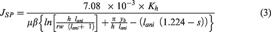
The specific productivity equation reported by Furui et al. (2003) is

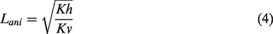
J_{S P} = \frac{7.08 \times 10^{- 3} \times K_{h}}{μ β \{l n [\frac{h l_{ani}}{r w (l_{ani} + 1)}] + \frac{π y_{b}}{h l_{ani}} - (l_{ani} (1.224 - s))\}}

(3)

The permeability anisotropy formula used is

L_{ani} = \sqrt{\frac{K h}{K v}}

(4)

Integration of equation (2) yields the fluid flow rate formula in the drain hole at point x as

Q_{o} (x) = \int_{0}^{x} J_{s p} [P_{r} - P_{w} (x)] d x

(5)

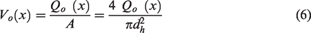
The formula for the average flow velocity in the drain hole at point x is given by Guo et al. (2007) as

V_{o} (x) = \frac{Q_{o} (x)}{A} = \frac{4 Q_{o} (x)}{π d_{h}^{2}}

(6)

Substituting equations (5) into (6) gives

V_{o} (x) = \int_{0}^{x} \frac{0.012 J_{s p} [P_{r} - P_{w} (x)] d x}{d_{h}^{2}}

(7)

The $V_{o} (x)$ is in ft/s while the dh is in inches and the pressures are in psi.

The first law of thermodynamics considering the pressure drop due to friction, fluid accumulation and kinetic energy is given in U.S engineering units as (Fadairo et al., 2015, 2018, 2020)

- d P_{w} (x) = \frac{2 f_{f} ρ v_{o}^{2} (x) d x}{g_{c} D_{h}} + \frac{2 ρ v_{o}^{2} (x)}{g_{c}} + \frac{2 ρ v_{o} (x) d x}{g_{c} Δ t}

(8)

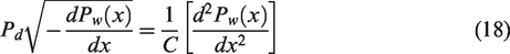
Rearranging in field units gives

{72dp}_{w} (x) = - \frac{0.373 f_{f} ρ_{o} v_{o}^{2} (x)}{d_{h}} d x + \frac{0.0311 ρ_{o} v_{o} (x)}{Δ t} d x + 0.0311 ρ_{o} v^{2}_{o} (x)

(9)

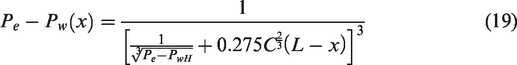
For simplicity sake, equation (9) can be simply re-arranged as

- 72 \frac{{dp}_{w} (x)}{d x} = v_{o}^{2} (x) (\frac{0.373 f_{f} ρ_{o}}{d_{h}} + \frac{0.0311 ρ_{o}}{v_{o}^{*} Δ t} + \frac{0.0311 ρ_{o}}{L})

(10)

Let v {}_{o}{^{*}} = \frac{0 .012 J_{s p}}{d_{h}^{2}} Δ p^{*^{}} L and Δ p^{*} = p_{e} - p_{w H}

(11)

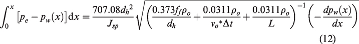
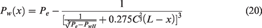
Substituting equation (7) into equation (10) and re-arranging, we have

\int_{0}^{x} [p_{e}^{} - p_{w}^{} (x)] d x = \frac{707.08 d_{h}^{2}}{J_{s p}} \sqrt{{(\frac{0.373 f_{f} ρ_{o}}{d_{h}} + \frac{0.0311 ρ_{o}}{v_{o}^{*} Δ t} + \frac{0.0311 ρ_{o}}{L})}^{- 1} (- \frac{d p_{w} (x)}{d x})}

(12)

Defining P_{e} - P_{w} (x) = P_{d}

(13)

\int_{0}^{x} [p_{d})] d x = \frac{707.08 d_{h}^{2}}{J_{s p}} \sqrt{{(\frac{0.373 f_{f} ρ_{o}}{d_{h}} + \frac{0.0311 ρ_{o}}{v_{o}^{*} Δ t} + \frac{0.0311 ρ_{o}}{L})}^{- 1} (- \frac{d p_{w} (x)}{d x})}

(14)

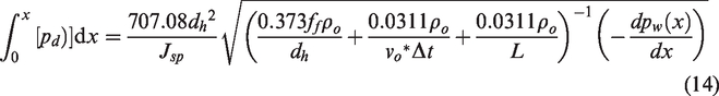
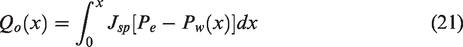
Take derivatives of equation (14) with respect to x and re-arranging, we have

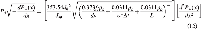
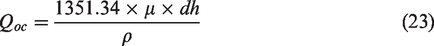
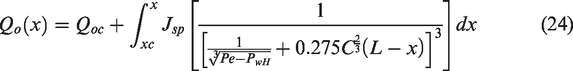
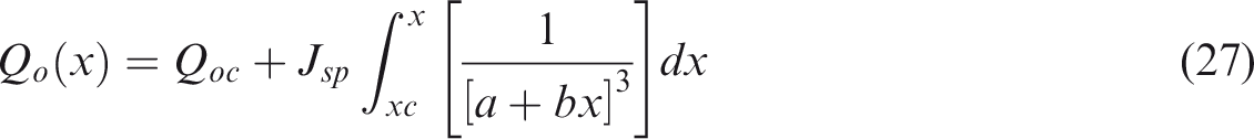
P_{d} \sqrt{- \frac{d P_{w} (x)}{d x}} = [\frac{353.54 d_{h}^{2}}{J_{s p}} \sqrt{{(\frac{0.373 f_{f} ρ_{o}}{d_{h}} + \frac{0.0311 ρ_{o}}{v_{o}^{*} Δ t} + \frac{0.0311 ρ_{o}}{L})}^{- 1}}] [\frac{d^{2} P_{w} (x)}{d x^{2}}]

(15)

Defining

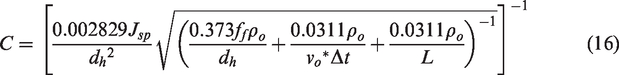
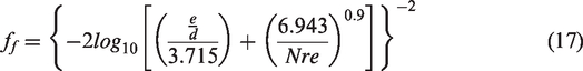
C = {[\frac{0.002829 J_{s p}}{d_{h}^{2}} \sqrt{{(\frac{0.373 f_{f} ρ_{o}}{d_{h}} + \frac{0.0311 ρ_{o}}{v_{o}^{*} Δ t} + \frac{0.0311 ρ_{o}}{L})}^{- 1}}]}^{- 1}

(16)

The fanning friction factor which depends on hole roughness and the Reynolds number which is defined by Jain correlation as

f_{f} = {\{- 2 \log_{10} [(\frac{\frac{e}{d}}{3.715}) + {(\frac{6.943}{Nre})}^{0.9}]\}}^{- 2}

(17)

Equation (15) can be written as

P_{d} \sqrt{- \frac{d P_{w} (x)}{d x}} = \frac{1}{C} [\frac{d^{2} P_{w} (x)}{d x^{2}}]

(18)

Equation (18) can be solved. Following the procedure reported by Guo et al. (2007), we have

P_{e} - P_{w} (x) = \frac{1}{{[\frac{1}{\sqrt[3]{P_{e} - P_{w H}}} + 0.275 C^{\frac{2}{3}} (L - x)]}^{3}}

(19)which can also be expressed as

P_{w} (x) = P_{e} - \frac{1}{{[\frac{1}{\sqrt[3]{P_{e} - P_{w H}}} + 0.275 C^{\frac{2}{3}} (L - x)]}^{3}}

(20)

Recall equation (5)

Q_{o} (x) = \int_{0}^{x} J_{s p} [P_{e} - P_{w} (x)] d x

(21)

Assuming the transition from laminar flow regime to turbulent flow regime can be overlooked, the fluid flow rate will therefore be a combination of both the laminar and turbulent flow regimes and equation (5) can therefore be expressed as

Q_{o} (x) = Q_{o c} + \int_{x c}^{x} J_{s p} [P_{e} - P_{w} (x)] d x

(22)

Assuming the critical Reynold number is 2000, an expression for critical flow rate is obtained as (Guo et al., 2007)

Q_{o c} = \frac{1351.34 \times μ \times d h}{ρ}

(23)

Substituting equation (20) into equation (22) gives

Q_{o} (x) = Q_{o c} + \int_{x c}^{x} J_{s p} [\frac{1}{{[\frac{1}{\sqrt[3]{P e - P_{w H}}} + 0.275 C^{\frac{2}{3}} (L - x)]}^{3}}] d x

(24)

Let

a = \frac{1}{\sqrt[3]{\Pr - Pwh}} + 0.2752 \times C^{\frac{2}{3}} \times L

(25)

b = - 0.2752 \times C^{\frac{2}{3}}

(26)

Hence we have

Q_{o} (x) = Q_{o c} + J_{s p} \int_{x c}^{x} [\frac{1}{{[a + b x]}^{3}}] d x

(27)

Integration of equation (27) yields

Q_{o} (x) = Q_{o c} + \frac{J_{s p}}{2 b} [\frac{1}{{[a + b x_{c}]}^{2}} - \frac{1}{{[a + b x]}^{2}}]

(28)At point

x = L

(29)

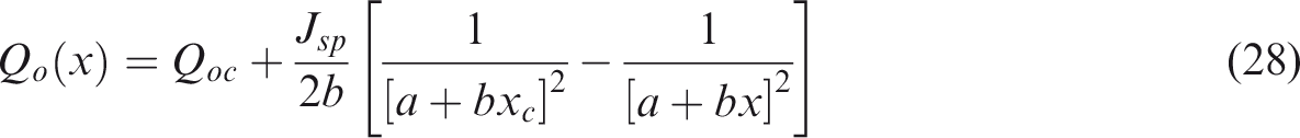
The final equation can be expressed as

Q_{o} (x) = Q_{o c} + \frac{J_{s p}}{2 b} [\frac{1}{{[a + b x_{c}]}^{2}} - \frac{1}{{[a + b L]}^{2}}]

(30)

Model analysis

This modified model is an extension of Guo et al. (2007) model to account for all flow behaviors that evident at the beginning of flow of fluid in pipe after shut in operation. The illustration to evaluate flow rate at the stabilized state after production time of 120 days using the modified equation has been demonstrated in Appendix 1.

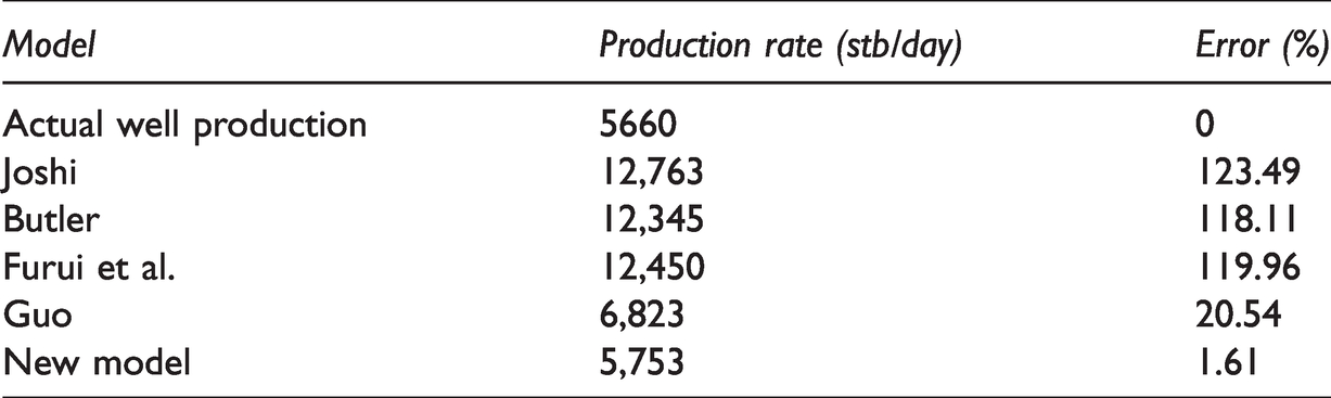
A field case information (Table 1) reported in the literature Guo et al. (2007) was taken into consideration in the calculation; the wellbore has a pay zone thickness of 131.2 ft, the length from the toe to the heel of the wellbore is 2438 ft with an effective drain-hole diameter of 5.5 in. with a well production rate of 5660 stb/day. The different models predicted different flow rates and the superiority of this model was evident as it gave a much better prediction using gauge measurement of the field case for benchmark. Table 2 shows a comparison of the flow rates calculated at stabilized state by the modified model and other existing models with their corresponding error percentage.

Table 1.

Fluid and reservoir parameters.

Pay zone thickness (ft.)	131.2
Boundary distance (ft.)	500
Horizontal permeability (md)	770
Vertical permeability (md)	254
Skin factor	0
Oil density (lbm/ft³)	55.97
Oil viscosity (cp)	0.5
Oil formation volume factor (rb/stb)	1.058
Reservoir pressure (psi)	932.5
Drain hole radius to sand face (ft.)	0.708
Effective drain hole diameter (in.)	5.5
Drain hole pressure at heel (psi)	025
Drain hole length (ft.)	2.438
Drain hole wall roughness (in.)	0.00024

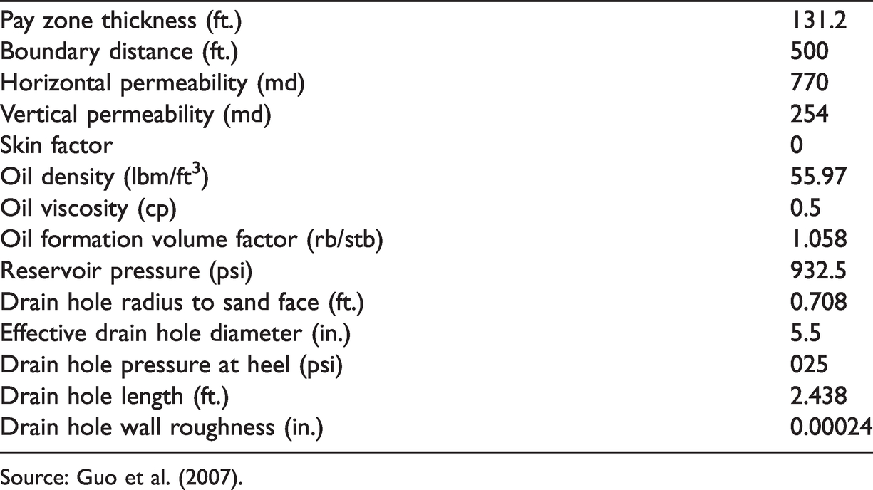
Source: Guo et al. (2007).

Table 2.

Final model comparison, after Guo et al. (2007).

Model	Production rate (stb/day)	Error (%)
Actual well production	5660	0
Joshi	12,763	123.49
Butler	12,345	118.11
Furui et al.	12,450	119.96
Guo	6,823	20.54
New model	5,753	1.61

Results analysis

The result obtained from modified model demonstrated the flow behaviors that are closer to realistic flow dynamic in oil and gas well after shut in as the flow changes from the non-stabilized to stabilized condition in the drain hole from the reservoir were established and reported in Figure 1. The results obtained in Figure 1 also show the effect of all neglected possible wellbore pressure losses such as losses due to accumulation term and kinetic term on flow phenomena in horizontal oil production well. It has been demonstrated from the outcomes of this study that the inconsistency in the results obtained by gauge and that obtained by the past developed models in the literature were not just because of the impact of pressure losses due to friction term as suggested by previous authors however may likely be caused by losses due to kinetic and accumulation experienced by the flowing fluid in a channel. The result from the modified model has been sufficiently more correct and demonstrated an error margin that is less than 2% validating with other past models that gave higher error margins after benchmarking with the gauge measurement value. This study gives reservoir engineer an exact and helpful device for estimating and easy assessment of oil wells production rate.

Figure 1.

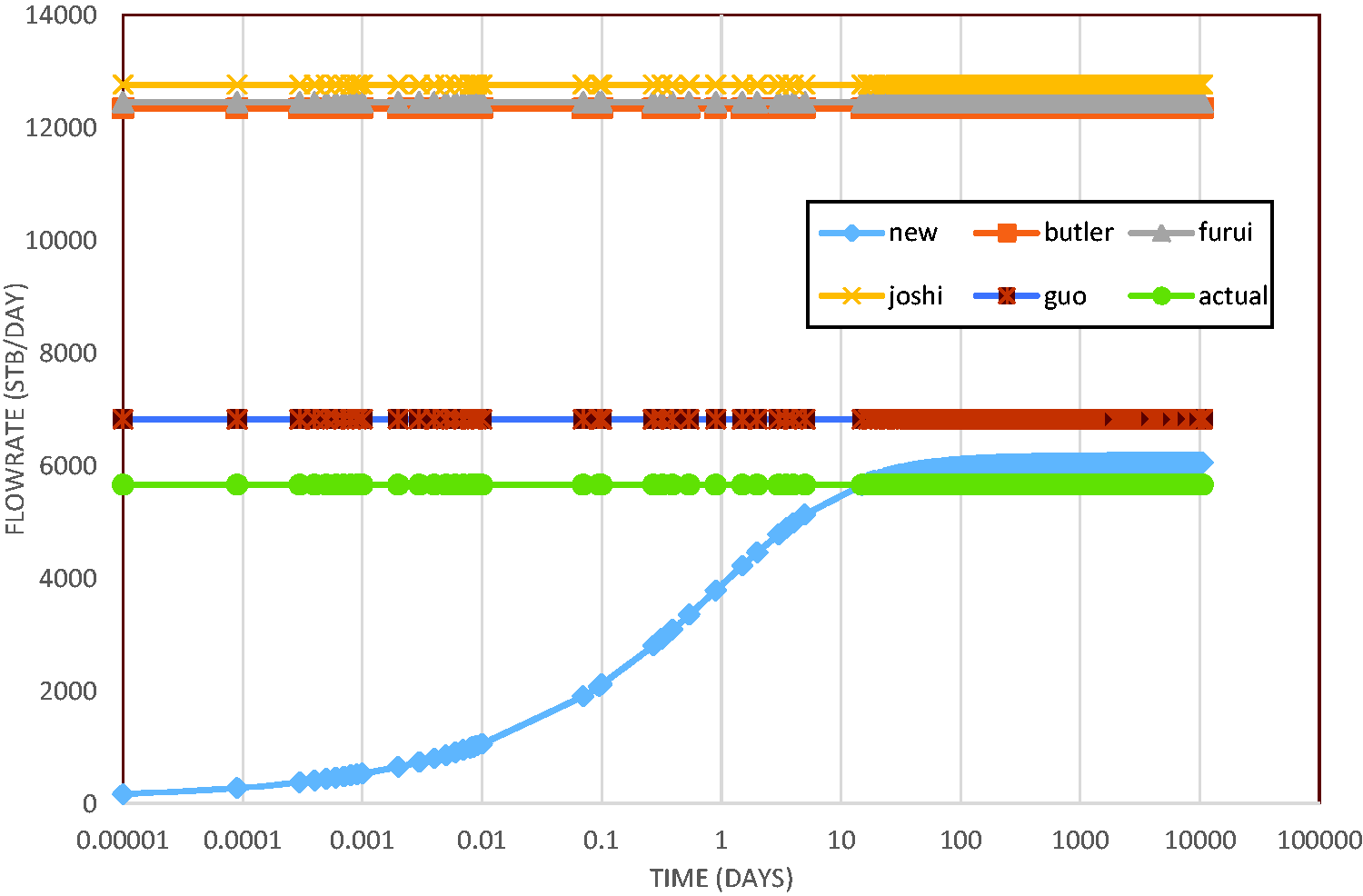
Flow rate calculated against time from existing models and the current model using actual field data for validation.

Figure 2 presents flowing pressure results at different production time and shows improvement over previous study as the initial unsteadiness experience in reality phenomena occurs at the onset of flow after shut-in in oil well was evident and assumptions previously neglected by previous studies were all considered.

Figure 2.

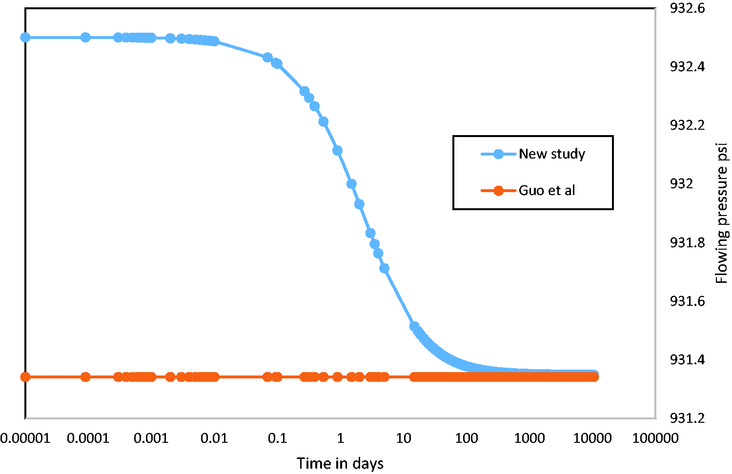
Flowing pressure against time calculated from past model and current model.

The modified concept gives functional relationship between flow rate and pressure transverse at any point in flowing well at any given production time as reported in Figures 3 and 4, respectively. Figures 3 and 4 have demonstrated high initial unsteadiness at the early of production time due to possible pressure losses encountered in long horizontal section of drain hole and decline gradually to match up the Guo et al. (2007) result as production time increases. This implies well bore pressure loss induced by accumulation term and kinetic term are responsible for higher unsteadiness experienced at the beginning of production and continue till approximately 21 days (504 h) where the flow becomes stabilize hence catch up with the Guo et al. (2007) that only considered losses due to friction. The study suggests that the huge pressure drop surge associated with initial unsteadiness encounter at the early flow of fluid after shut-in should be incorporated as a key factor during material design of production tubing and pipe to avoiding high pressure induced burst.

Figure 3.

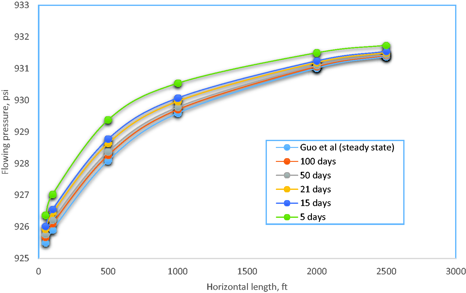
Shows flowing pressure against horizontal length at production time compared with past model at steady state.

Figure 4.

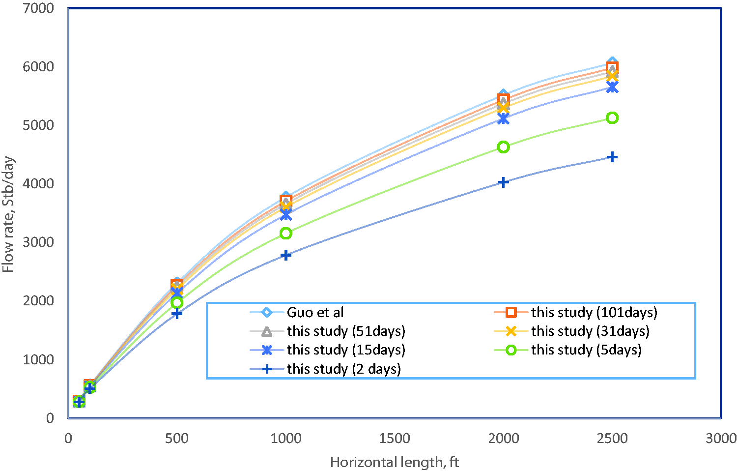
Shows flow rate against horizontal length at production time compared with past model at steady state.

Conclusion

The newly developed model for predicting flow rate in horizontal drain hole has revealed that the early available models for this purpose can only be valid for short horizontal drain hole where accumulation and kinetic induced restriction are negligible. The new study presents an exact model that includes essential restriction terms that were previously neglected by the past investigators. Huge discrepancies obtained when compared the past models with the actual field value measured indicate that optimum field development and economic analysis are difficult to achieve using the existing models. The following conclusions can be deduced based on sample field scenario investigated using the newly developed model.

The new model can be used to simulate the flow rate for long horizontal oil well and established functional relationship that produced the most accurate result that gives percentage error of 1.61% compared with previously developed models of Joshi, Butler, Furui et al. and Guo et al. steady state models that reported percentage errors of 123.49, 118.11, 119.96, and 20.54, respectively, in their literature using the real life value reported in Guo et al. (2007) as the benchmark.

The results obtained from the newly developed model are practically represented as the initial unsteadiness phenomena experience in real life was clearly demonstrated at the onset of flow after shut-in in a long horizontal well.

This study gives an improvement over previous investigations as the vital assumptions previously neglected by previous studies on flow rate for long horizontal well were all considered. However further validation with experimental and field results that showcase the transient flow behavior is recommended to ascertain the accuracy of the improved model at the transient flow region.

The study suggests to the completion engineer that the huge pressure drop surge associated with initial unsteadiness encounter at the early flow of fluid after shut-in should be considered as a key factor during the material design of production tubing and pipe. This enable the proper management of risk associated with high pressure induced burst that may occur at the onset of fluid flow under high pressure-high temperature condition.

Limitation

This study was based on the assumption of single-phase flow, hence the new model can only be valid for horizontal oil well production system. The version of this study that is valid for horizontal gas production system has been reported in previous work done by Fadairo et al. (2019). Further research need to be done to accommodate horizontal multiphase production system and to demonstrate the effect of flow regime on the horizontal well performance.

Footnotes

Declaration of conflicting interests

The author(s) declared no potential conflicts of interest with respect to the research, authorship, and/or publication of this article.

Funding

The author(s) received no financial support for the research, authorship, and/or publication of this article.

ORCID iD

Adesina Fadairo

Appendix 1. Comparison of mathematical models with field data

The outcome of the study have established functional relationship that produced more realistic and accurate models that gives percentage error of 1.61 compared with previously developed Joshi, Butler, Furui et al. and Guo et al. models that reported percentage errors of 123.49, 118.11, 119.96 and 20.54 respectively in their literature using the real life value as the benchmark.

References

Al-Rheawi

(2019) Revisiting current techniques for analyzing reservoir performance: a new approach for horizontal wellbore pseudo-steady state productivity index. SPE Journal 24(1): 71–91.

Al-Rheawi

(2018) The optimal reservoir configuration for maximum productivity index of gas reservoirs depleted by horizontal wells under Darcy and non-Darcy flow conditions. Journal of Natural Gas Science and Engineering 49: 179–193.

Butler

(1994) Horizontal wells for the recovery of oil, gas and bitumen. Petroleum Monograph No. 2. Petroleum Society of CIM.

Davarpanah

Shirmohammadi

Mirshekari

, et al. (2019) Analysis of hydraulic fracturing techniques: hybrid fuzzy approaches. Arabian Journal of Geosciences 12(13): 402.

Davarpanah and Mirshekari (2019) Mathematical modeling of injectivity damage with oil droplets in the waste produced water re-injection of the linear flow. The European Physics Journal Plus 134: 180.

Davarpanah

Mirshekari

Behbahani

, et al. (2018) Integrated production logging tools approach for convenient experimental individual layer permeability measurements in a multi-layered fractured reservoir. Journal of Petroleum Exploration and Production Technology 8(3): 743–751.

Davarpanah

Mirshekari

Razmjoo

(2020) A parametric study to numerically analyze the formation damage effect. Energy Exploration & Exploitation 38(2): 555–568.

Dikken

(1990) Pressure drop in horizontal wells and its effect on production performance. Journal of Petroleum Technology 42(11): 1426–1433.

Economides

Deimbachor

Brand

, et al. (1991) Comprehensive simulation of horizontal well performance. SPE Formation Evaluation 6(4): 418–426.

10.

Fadairo

Adebowale

Gbadegesin

(2019) A modified predictive model for estimating gas flow rate in horizontal drain hole. Petroleum 5(1): 35–41.

11.

Fadairo

Adeyemi

Ogunkunle

(2020a) An improved semi analytical approach for predicting horizontal and multilateral well performance [Chapter 4]. In: Sid-Ali Ouadfeul and Leila Aliouane (eds), Oil and Gas Well. London, Uk: InTech Publisher, 2020.

12.

Fadairo

Anawe

Orodu

, et al. (2016) An improved model for estimating productivity of horizontal drain-hole. In: Paper SPE 184264-MS presented at the SPE Nigeria annual international conference and exhibition, Nigeria, 2–4 August 2016.

13.

Fadairo

Churchill

Olugbenga

(2011) Modeling productivity index for long horizontal well. Journal of Energy Resources Technology 133(3): 033101.

14.

Fadairo

Falode

Nwosu

(2015) A new model for predicting liquid loading in a gas well. Journal of Natural Gas Science and Engineering 26: 1530–1541.

15.

Fadairo

Gbadegesin

Temitope

, et al. (2018) A realistic model for estimating productivity index of vertical well using wellhead data. In: SPE Paper 193506, SPE Nigerian annual international conference and exhibition, Lagos, 6–8 August 2018.

16.

Fadairo

Omole

Falode

(2008) Effect of oilfield scale deposition on mobility ratio. In: CIPC/SPE international conference, Canada, SPE 114488.

17.

Fadairo

Rasouli

Adelakun

, et al. (2020b) An improved hydraulics model for aerated fluid underbalanced drilling in vertical wells. Upstream Oil and Gas Technology 5: 100009.

18.

Folefac

Archer

Issa

, et al. (1991) Effect of pressure drop along horizontal wellbores on well performance. In: Paper SPE 23094 presented at the SPE offshore Europe conference, Aberdeen, UK, 3–6 September 1991.

19.

Furui

Zhu

Hill

(2003) A rigorous formation damage skin factor and reservoir inflow model for a horizontal well. SPE Production & Facilities 18(3): 151–157.

20.

Giger

(1985) Horizontal wells production techniques in heterogeneous reservoirs. In: Paper SPE 13710 presented at the SPE Middle East oil technical conference and exhibition, Bahrain, 11–14 March 1985.

21.

Goode

Kuchuk

(1991) Inflow performance of horizontal wells. SPE Reservoir Engineering 6(3): 319–323.

22.

Guo

Zhou

Liu

, et al. (2007) A rigorous analytical model for fluid flow in drain holes of finite conductivity applied to horizontal and multilateral wells. In: Paper SPE 106947, presented at the SPE 2007 production operations symposium, Oklahoma City, OK, 31 March 2007.

23.

Guo

Liu

, et al. (2020) Physical simulation of hydraulic fracturing of large-sized tight sandstone outcrops. SPE J 1–22. SPE-204210-PA. Available at: www.onepetro.org/journal-paper/SPE-204210-PA.

24.

Hill

Zhu

(2008) The relative importance of wellbore pressure drop and formation damage in horizontal wells. SPE Production & Operations 23(2): 232–240.

25.

Joshi

(1988) Augmentation of well productivity with slant and horizontal wells. Journal of Petroleum Technology 40(6): 729–739.

26.

Kamkom

Zhu

(2005) Evaluation of two-phase IPR correlations for horizontal wells. In: Paper SPE 93986 presented at the SPE production and operations symposium, Oklahoma City, Oklahoma, 17–19 April 2005.

27.

Kuchuk. Goode Wilkinson Michael ‘Pressure-Transient Behavior of Horizontal Wells With and Without Gas Cap or Aquifer’. SPE Formation Evaluation 6(1): 86–94. DOI: 10.2118/17413-PA

28.

Landman

(1994) Analytical modeling of selectively perforated horizontal wells. Journal of Petroleum Science and Engineering 10(3): 179–188.

29.

Liu

Chen

Guan

, et al. (2019) Layout optimization of large-scale oil-gas gathering system based on combined optimization strategy. Neurocomputing 332: 159–183.

30.

Moosavi

S R

Vaferi

Wood

D A

(2020) Auto-detection interpretation model for horizontal oil wells using pressure transient responses. Advances in Geo-Energy Research 4(3): 305–316.

31.

Nesic

Zolotukhin

Mitrovic

, et al. (2020) An analytical model to predict the effects of suspended solids in injected water on the oil displacement efficiency during waterflooding. Processes 8(6): 659.

32.

Novy

(1995) Pressure drop in horizontal wells: when can they be ignored. SPE Reservoir Engineering 10(1): 29–35.

33.

Ouyang

L-B

Huang

(2005) An evaluation of well completion impact on the performance of horizontal and multilateral wells. In: Paper SPE 96530 presented at the SPE annual technical and exhibition, Dallas, Texas, pp.9–12.

34.

Ozkan

Raghavan

Joshi

S D

(1989) Horizontal-well pressure analysis. SPE Formation Evaluation 4(4): 567–575.

35.

Ozkan

Sarica

Haciislamoglu

, et al. (1993) The influence of pressure drop along the wellbore on horizontal productivity. In: Paper SPE 25502 presented at the SPE production operations symposium, Oklahoma City, Oklahoma, 21–23 March 1993.

36.

Penmatcha

Arbabi

Aziz

(1997) Effects of pressure drop in horizontal wells and optimum well length. In: Paper presented at the SPE production operations symposium, Oklahoma City, Oklahoma, 9–11 March 1997.

37.

Renard

and and Duppy

(1990) Influence of formation damage on the flow efficiency of horizontal wells. In: Presented at formation damage control symposium, Lafayette, Louisiana, 22–23 February 1990, SPE Paper No.9414.

38.

Siu

Subramanian

(1995) A complete hydraulics model for horizontal wells. In: Paper SPE 29134 presented at the SPE symposium on reservoir simulation, San Antonio, Texas, 12–15 February 1995.

39.

Sun

Davarpanah

(2020) Application of symmetry law in numerical modeling of hydraulic fracturing by finite element method. Symmetry 12: 1122.

40.

Tabatabaei and Ghalambor (2011) A New Method To Predict Performance of Horizontal and Multilateral Wells. SPE production & operations 26(1): 75–87

41.

Yildiz

Ozkan

(1998) A simple correlation to predict wellbore pressure drop effects on horizontal well productivity. In: Paper SPE 48938 presented at the SPE ATCE, New Orleans, Louisiana, 27–30 September 1998.

42.

Yuan

Sarica

Brill

(1998) Effect of completion geometry and phasing on single phase liquid flow behavior in horizontal wells. In: Paper SPE 48937 presented at the SPE ATCE, New Orleans, Louisiana, 27–30 September 1998.

43.

Zhong

Yang

Yin

, et al. (2020) Role of alkali type in chemical loss and ASP-flooding enhanced oil recovery in sandstone formations. SPE Reservoir Evaluation & Engineering 23(2): 431–445.

Modelling flow for finite conductivity in long horizontal oil wells

Abstract

Keywords

Introduction

Governing equations

The derivation

Model analysis

Results analysis

Conclusion

Limitation

Footnotes

Declaration of conflicting interests

Funding

ORCID iD

Appendix 1. Comparison of mathematical models with field data

References