Sage Journals: Discover world-class research

Abstract

Fiji is located in the South Western part of the Pacific between latitude 18° S and longitude 179° E. In 2018, Fiji has spent approximately FJD 800 million in importing fossil fuel to meet the rising energy demand in the country. In the previous year’s several solar PV and wind resource assessments has been done and results obtained indicated that there is a potential for grid connected electricity generation using recommended resources. This study was carried out in the Nasawana Village (16°55.3 S and 178°47.4 E) to determine the options to use electricity derived from the wind. Wind analysis was carried out using Wind Atlas Analysis and Application Program (WAsP) that predicted the wind speed of 6.96 ms⁻¹ and a power density of 256 Wm⁻² at 55 m a.g.l. The annual energy production predicted for a single wind turbine (Vergnet 275 kW) is approximately 631.6 MWh with a capacity factor of 26%. The cost of energy per kWh is estimated as FJD 0.10 with a payback period of 7 years.

Keywords

Wind Atlas Analysis and Application Program annual energy production cost of energy Vergnet 275 kW

Introduction

Current developments of wind in the pacific

Fossil fuels cater for around 72.7% (REN21, 2020) of the energy needs globally that have profound impact on climate change. Renewable energy delivers approximately 27.3% (REN21, 2020) of the total energy generated worldwide comprising of biomass, modern renewables, geothermal, hydropower, wind, solar and biofuels. The installed wind capacity was approximately 60 GW in 2019, more than 10% from 2018 and brought the global total capacity to 651 GW at the end of 2019 (REN21, 2020). According to the World Bank (2020) statistics that around 99.6% of population in Fiji have access to electricity. Fiji’s Electricity demand as of 2018 was approximately 1033 GWh of which 43% was generated by diesel generators (fossil fuel) and 57% by renewable energy resources comprised of hydro, wind and solar (EFL, 2018). This demand is expected to increase substantially in the near future. Most of the rural settlements in Fiji do not have access to grid electricity because of its remoteness and low population density. However, with present National Energy Policy, the options of stand-alone and mini grid systems are evaluated under the rural electricity projects. Wind resource assessments and wind turbine installation (Table 1) have been carried out in the South Pacific region in the past and continuous resource assessments of renewable energy are being carried out by the researchers. It also shows that Fiji is amongst the highest producer of electricity using renewable resources in the pacific.

Table 1.

Wind Farms in the Pacific Island Countries (Pacific Energy Country Profiles, 2016).

	Wind farms
Country	Location	Capacity (MW)	Number of turbines	Hub height (m)	Commissioning Year	RE contribution (%)	Total RE generation (MWh)
Fiji	Butoni	10	37 Vergnet 275 kW	55	2008	65	585000
Vanuatu	Devils Point	3	11 Vergnet 275 kW	55	2009	18.9	11907
New Caledonia	Prony Kafeate	2.2 11.55	10Vergnet 220 KW 42 Vergnet 275 kW	50 55	2008 2005	6	17772700
Tahiti	–	11.55	42 Vergnet 275 kW	55	2006	33.9	182043
Samoa	–	0.55	2 Vergnet 275 kW	55	–	60	73680
Cook Islands	–	0.04	GEV-10/20 type	30	2003	15	4763
Tonga	Nakolo	0.011	Gaia	18.4	2013	26	46240
Kiribati	–	–	–	–	–	10	2300
Nauru	–	–	–	–	–	3.2	1014
Niue	–	–	–	–	–	13	429
Solomon Islands	–	–	–	–	–	5	3900

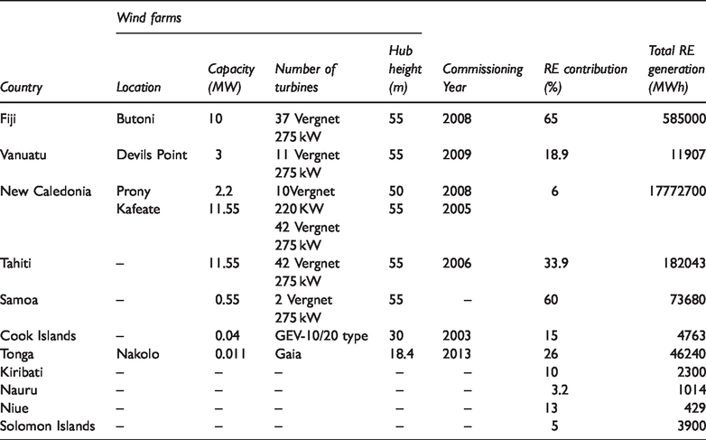
Several studies (Kumar and Nair, 2012, 2013; Kumar and Prasad, 2010) have been carried out to determine the wind regime around Fiji. Rafique et al. (2018) stated that the wind energy mix is feasible, both technically and economically for developing countries to ease their dependence on fossil fuel.

Kumar and Prasad (2010) have detailed Fijis only hybrid wind, solar and diesel power generating system (comprised of mixed electricity generation with wind, solar and diesel) in Nabouwalu, Vanua Levu, commissioned in 1997 by the Pacific International Center for Higher Technology Research (PIHCTR). However, due to inadequate maintenance of the renewable energy components (wind and PV) the hybrid system is currently not operational. The diesel component is providing the electricity needs of the consumers.

Fiji spends approximately FJD 800 million of its total import on mineral fuels. This burdens the national budget of FJD 4.65 billion, thus allowing less to be spent on essentials like health and education. Hence, there is a need for greater renewable energy mix in the mainstream supply of energy.

Fiji Department of Energy (FDoE) has conducted many wind resource assessments at Qamu, Korotogo, Vanatova, Waibongi, Kavakava, Tamuku, Vunisea, Vadravadra, Nacamaki, Wainitaku and Benau on Vanua Levu and Viti Levu. Analysis carried out on these sites suggested that all these sites are averagely suited for producing electricity. The objective of this research was to find out the potential of wind energy resource of Nasawana Village in Nabouwalu, Vanua Levu and determine its economic viability. A summary of the energy production (Figure 1) for some of the PICs. Fiji is amongst the highest producer of electricity using renewable resources.

Figure 1.

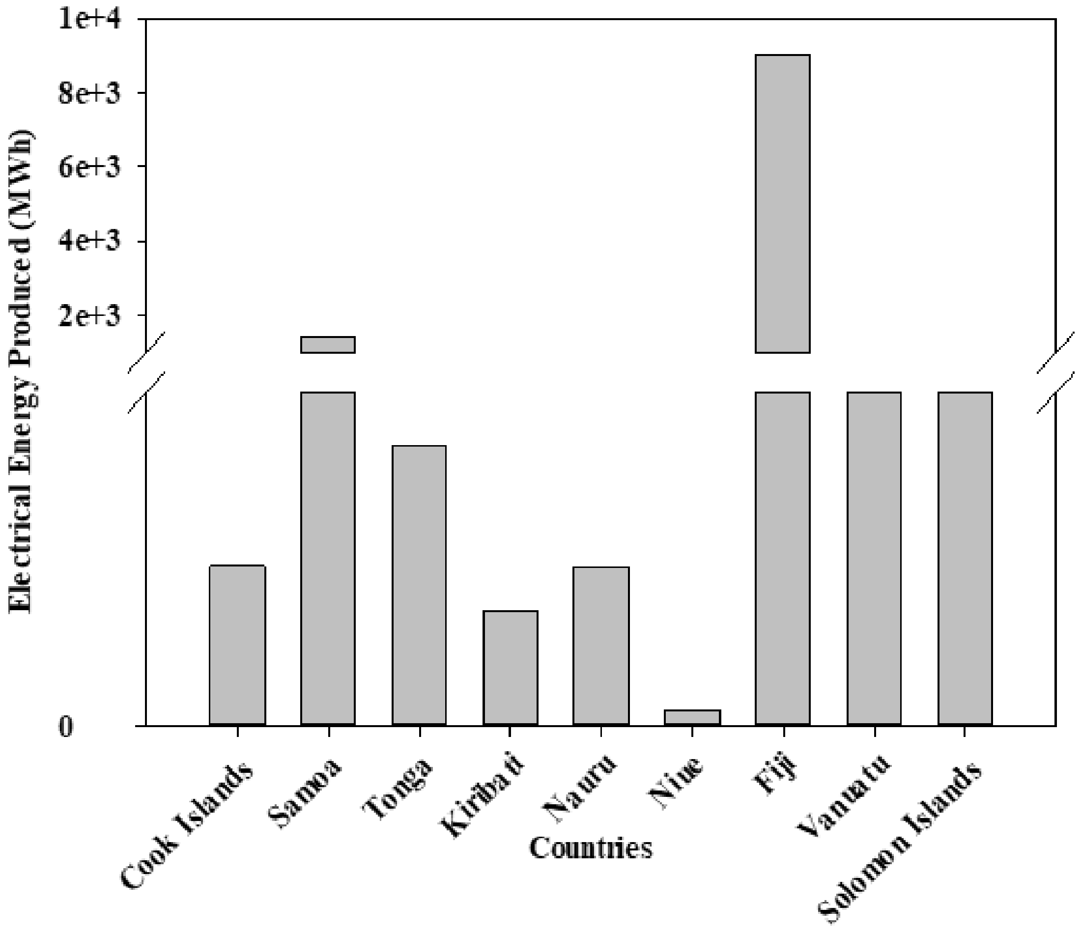
Summary of energy production for some PICs (Pacific Energy Country Profiles, 2016).

South pacific wind climatology

The South Pacific region is exposed to South East trade winds. The wind blows from the high pressure zone in subtropics latitudes between 30^° to 35^° South towards low pressure zone around the equator. Countries near to the equator where there is lowlands (Fiji, Solomon Islands, Kiribati, Vanuatu, Cook Islands, Tonga, Samoa and Niue), have summer season whole of the year with ideal fluctuations in temperature and atmospheric pressure.

Fiji is geographically located at 18° S and 179° E which consists of more than 300 Islands with total land area of 18,274 km². The Fiji Islands energy demand increases at a rate of 5% per year with an increasing population of approximately 884,887 as of 2017 (Fiji Bureau of Statistics, 2017). Fiji is ranked 133rd in terms of petroleum consumption in world totaling to approximately ten thousand barrels per day with 1.33 million metric tonnes of Carbon dioxide emission annually (Clean Development Mechanism Investors Guide, 2012).

Wind resource estimate using WAsP

Wind Atlas Analysis and Application Program (WAsP) was established by the Technical University of Denmark (DTU) in 1987 and is continuously upgraded to improve the performance of the model, in particular when dealing with complex terrain and atmosphere. WAsP has become the industry standard for wind resource assessment and siting of wind turbines and wind farms. This linear arithmetical model is used to assess vital topographies of a wind farm. WAsP uses Weibull distribution to evaluate wind data and projects it over areas of similar climate to its reference site. Rehman et al. (2020b) using WAsP determined wind energy potential at three cities in Tamil Naidu. There are numerous wind resource assessment projects globally that used WAsP software for wind energy estimation.

Other researchers, Khadem and Hussain (2006) used WAsP software to develop a wind atlas and wind resource map at an altitude of 50 m a.g.l for Kutubdia Island in Bangladesh. Taking into consideration of roughness and terrain effects, the results obtained suggested that the average annual wind speed for the site varied in the range of 5.1 – 5.8 ms⁻¹. The power density obtained was 200 Wm⁻², which is ideal for installation of a small turbine. Shata and Hanitsch (2006) used WAsP program for a technical assessment for two commercial turbines of 300 kW and 1 MW capacity. The 1 MW had the estimated power production of 2718 MWh annually at El Dabaa, Egypt with cost of energy as 2 €cent/kWh which was significantly low. It was concluded by the authors that Egypt has a promising wind regime and is economically viable.

In Fiji, Kumar and Nair (2012) proposed a potential wind farm which can be placed in Waniyaku state in Taveuni, Fiji. Analysis was done using one-year wind data using WAsP. It was found out that Waniyaki has a good wind regime with mean of 6.73 ms⁻¹ and mean power density of 266 Wm⁻² at 30 m a.g.l. It also suggested that a wind farm with four 275 kW wind turbines will have mean annual energy production (AEP) of 1.57 GWh at cost of energy as FJD 0.17/kWh. However, authors recommended more than three years of data is necessary for a better estimate of the economics. Kumar and Nair (2013) proposed a 2 turbines wind park for Benau, Savusavu on Vanua Levu. The analysis using WAsP showed a mean wind regime of 6.34 ms⁻¹ and wind power density of 590 Wm⁻² at a height of 30 m a.g.l. A comparison was made between Vergnet 275 kW wind turbine and Vesta V 27 whereby cost of energy for both turbines calculated were same. However, Vergnet 275 kW would produce more energy. WAsP also verified that a wind farm with a pair of Vergnet 275 kW would gather annual energy production (AEP) of 769 MWh at FJD 0.08/kWh with a cost to benefit ratio of 1.38, payback period of 5 years, and internal rate of return (IRR) of 21.3%.

Apart from standard software used for wind analysis, manual analysis using empirical, maximum likelihood, modified maximum likelihood, energy pattern and graphical techniques are used to obtain Weibull parameters. Researchers, Hulio et al. (2019), Rehman et al. (2020a), Bassyouni et al. (2015) and Shoaib et al. (2019) have successfully used the above techniques to analyze wind distribution at various locations.

Baseer et al. (2017) using multi-criteria decision making (MCDM) approach based on GIS modelling determined the most suitable wind farm location in the Kingdom of Saudi Arabia.

This paper presents the potential of wind energy resources around Nasawana Village in Nabouwalu, on the Island of Vanua Levu in Fiji. The seasonal, diurnal deviations of wind are analyzed. The energy distribution in relation to wind direction is also studied. The WAsP simulation results are presented estimating the average wind speeds and power density for the study site. The economical analysis of the site is carried out using Vergnet 275 kW wind turbine.

Wind energy economics

Kumar and Nair (2013) outlined that future value of wind investment C made today as

A_{1} = C {(1 + i)}^{2}, A_{3} = C {(1 + i)}^{3}, L, A_{n} = C {(1 + i)}^{n}

(1)

where, A_1, A₂, A₃, —, A_n indicate the value in the 1st, 2nd, 3rd, —, and nth year and L denotes the Principal or amount of loan. Here i is the interest rate or as more commonly termed, the discounting rate.

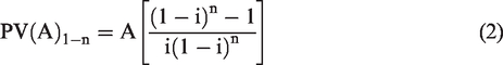
Thus the accumulated present value of all the payments put together is simplified as

PV {(A)}_{1 - n} = A [\frac{{(1 - i)}^{n} - 1}{i {(1 - i)}^{n}}]

(2)

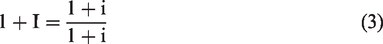
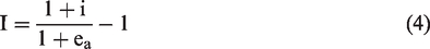
The discount rate corrected for inflation is termed as the real rate discount (I) which can be evaluated by

1 + I = \frac{1 + i}{1 + i}

(3)

where, r is the rate of inflation.

The real rate of discount, adjusted for both the inflation and escalation is then given by

I = \frac{1 + i}{1 + e_{a}} - 1

(4)

where, the apparent rate e_a is combination of the escalation rate e with the inflation r which is given by

e_{a} = \{(1 + e) (1 + r)\} - 1

(5)

Hence, the yearly cost of operation of the project is

NPV (C_{A}) = \frac{NPV {(C_{A})}_{1 - n}}{n} = \frac{C_{I}}{n} \{1 + m [\frac{{(1 + I)}^{n} - 1}{I {(1 + I)}^{n}}]\}

(6)

where, C_I is the investment is the operation and maintenance cost as a % of initial investment and NPV–(C_A) _1-n is the accumulated net present value of all the cost is given by

NPV {(C_{A})}_{1 - n} = C_{I} \{1 + m [\frac{{(1 + I)}^{n} - 1}{I {(1 + I)}^{n}}]\}

(7)

The energy generated by the turbine in a year is

E_{I} = 8760 P_{R} C_{F}

(8)

where, P_R is the rated power and C_F is the capacity factor of the turbine

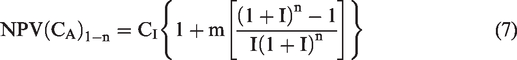
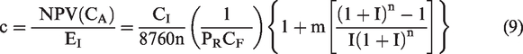
Hence, the cost of a unit (kWh) of wind-generated electricity is given by

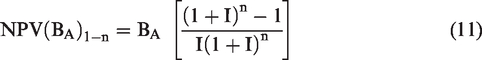
c = \frac{NPV (C_{A})}{E_{I}} = \frac{C_{I}}{8760 n} (\frac{1}{P_{R} C_{F}}) \{1 + m [\frac{{(1 + I)}^{n} - 1}{I {(1 + I)}^{n}}]\}

(9)

Thus, the net present value is given by

NPV = NPV {(B_{A})}_{1 - n} - \{C_{I} + NPV {(C_{A})}_{1 - n}\}

(10)

where, the project delivers a benefit of B_A annually through electricity sales, then the accumulated present value of all benefits over the life of the project is

NPV {(B_{A})}_{1 - n} = B_{A} [\frac{{(1 + I)}^{n} - 1}{I {(1 + I)}^{n}}]

(11)

Benefit cost ratio (BCR) is the ratio of the accumulated present value of all the benefits to the accumulated present value of all costs, including the initial investment can then be calculated as

BCR = \frac{NPV {(B_{A})}_{1 - n}}{C_{I} + NPV {(C_{A})}_{1 - n}}

(12)

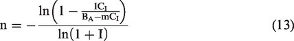
Payback period (PBP) is the year in which the net present value of all costs equals with the net present value of all benefits. Hence, PBP indicates the minimum period over which the investment for the project is recovered. Thus, the number of years, n, required to payback is determined by equating equation (10) to zero.

n = - \frac{\ln (1 - \frac{I C_{I}}{B_{A} - m C_{I}})}{\ln (1 + I)}

(13)

The internal rate of return (IRR) is the discount rate at which the accumulated present value of all the costs equals to that of the benefits. Hence, with IRR as the discount rate, the net present value of a project is zero. It is the maximum rate of interest that the investment can earn. IRR is the interest rate up to which we can afford to arrange the capital for the project. Thus equating equation (10) to zero and replacing I with IRR,

B_{A} \times [\frac{{(1 + IRR)}^{n} - 1}{IRR {(1 + IRR)}^{n}}] = C_{I} \times \{1 + m [\frac{{(1 + IRR)}^{n} - 1}{IRR {(1 + IRR)}^{n}}]\}

(14)

Description of the study site

The main study site Nasawana Village (Figure 2) is located at 16^°55.34 and 179^°47.39 in Bua Province on Vanua Levu. Nasawana Village is around 24 km from Vanua Levu’s main port of entry Nabouwalu and access to the site is through dirt road and there is no transmission grid. Nasawana village has a population of approximately 200 and use a diesel generation for electricity. The villagers are dependent on sea and root crops for their survival.

Figure 2.

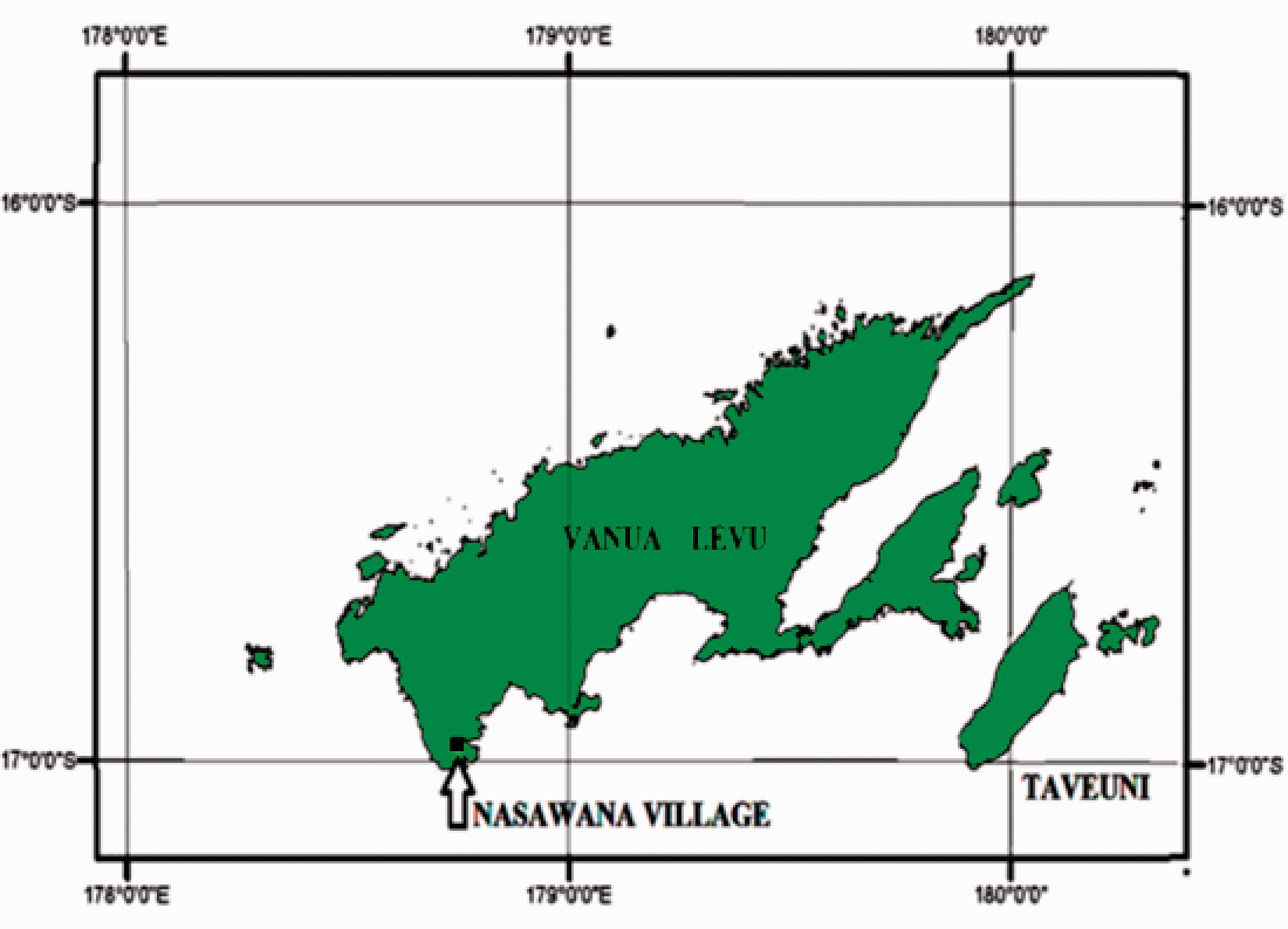
Nasawana Village (Adapted: Government map shop, Department of Lands and Survey, Fiji).

Methodology

Instrumentation, data recording and acquisition

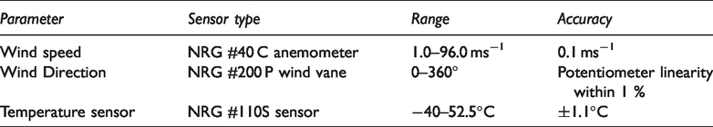
To monitor wind speed and wind direction at the Nasawana site a NRG #40 C anemometer and wind vane #200 P were mounted at 34 m and 20 m above the ground level (a.g.l) on the tower. The characteristics of the instruments (Table 2) shows the sensor type, range and their accuracy. The wind speed and the wind direction measurements were recorded continuously at every 10 minutes’ interval from March 2012 to June 2013. The data from the instruments were recorded using a NRG SymphoniePLUS data logger. The data were then transferred via iridium satellite to, The University of the South Pacific’s (USP) KOICA data repository.

Table 2.

Measuring sensor properties.

Parameter	Sensor type	Range	Accuracy
Wind speed	NRG #40 C anemometer	1.0–96.0 ms⁻¹	0.1 ms⁻¹
Wind Direction	NRG #200 P wind vane	0–360°	Potentiometer linearity within 1 %
Temperature sensor	NRG #110S sensor	−40–52.5°C	±1.1°C

The data were analyzed using industry-standard Wind Atlas Analysis and Application Program (WAsP) version 10 software package developed by DTU wind energy, Denmark. Based on the estimated electricity requirement and the observed wind data, possible installation of a wind turbine using Vergnet 275 kW was analyzed. An enclosed area of 25 km² around the monitoring site was analyzed for placement of a 275 kW wind turbine. The time-series of wind speed and wind direction data were converted into a table which portrayed a time-independent summary of the conditions found at the measuring site. All pertinent data were supplied and WAsP created an OWC report in HTML format. This report provided the general outline of the data supplied with any computations it carried out. The elevation and roughness values were provided and the map of Nasawana village was digitized using the WAsP map editor. WAsP used vector map specific to the terrain surface elevation represented by the contour heights and roughness lengths by roughness change lines (Troen and Petersen, 1989).

The porosity of the obstacles was selected based on the types of obstacles. The turbine generator and the digitized map were common for the entire project and were added as the child of the project. The Annual Energy Production (AEP) of Vergnet 275 kW turbine was estimated using WAsP, however it could be determined using the swept area of the rotor method, the power curve method or using manufactures’ estimates. Several studies reported in literature used anemometers and wind wanes, however, Rehman et al. (2018) successfully used LiDAR technique to determine the wind speed and power characteristics at King Fahd University.

Result and discussion

The data gathered were analyzed to determine wind energy potential at the study site. The average wind speed for the period of 15 months was calculated using:

u = \frac{1}{Δ t} \int_{0}^{Δ t} u d t

(15)

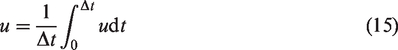
Considering an assumption that Δt = N_s Δt, over a number of sample wind speeds collected. The average wind speed is computed as:

u = \frac{1}{N_{s}} \sum_{i = 1}^{N_{s}} (u_{i})

(16)

where Ns = number of samples throughout individual short-term interval. u_i = wind speed (ms⁻¹).

Nasawana village wind data analysis

Daily wind speed analysis

The daily wind speed pattern at Nasawana was investigated for each month. The daily average wind speed (Figure 3) shows the magnitude in each day’s variation.

Figure 3.

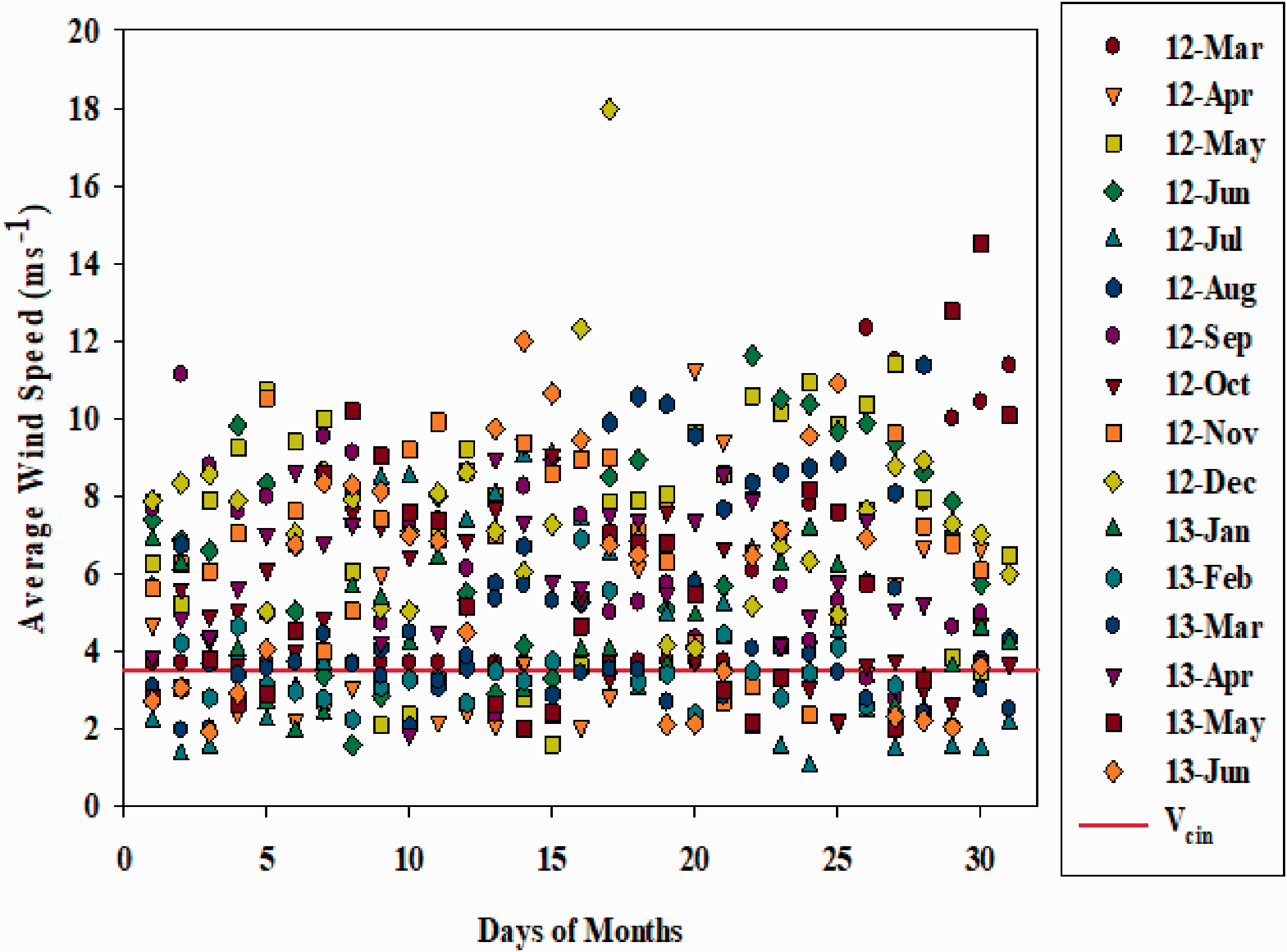
Wind speed distribution on same days of each month (March 2012 to June 2013) at 34 m a.g.l.

From Figure 3 it is clearly evident that most of the daily average wind speed is greater than the cut- in speed of 3.5 ms⁻¹ for Vergnet 275 kW turbine. Thus, it is predictable that this turbine would yield power most of the time. Calculations suggest that this turbine would produce power for approximately 72% of the time where the daily average wind speed is greater than 3.5 ms⁻¹. The highest average wind speed (17.97 ms⁻¹) recorded was for the month of December 2012 due to tropical cyclone Evans. The lowest average wind speed (1.92 ms⁻¹) was recorded in June. The cause of high and low wind speeds were due to high and low pressure that affected the Fiji group during those months.

The wind statistics at Nasawana (study site) (Figure 4) measured between March 2012 and June 2013 shows the annual variation with respect to the cut-in (V_cin) of a 275 kW Vergnet wind turbine.

Figure 4.

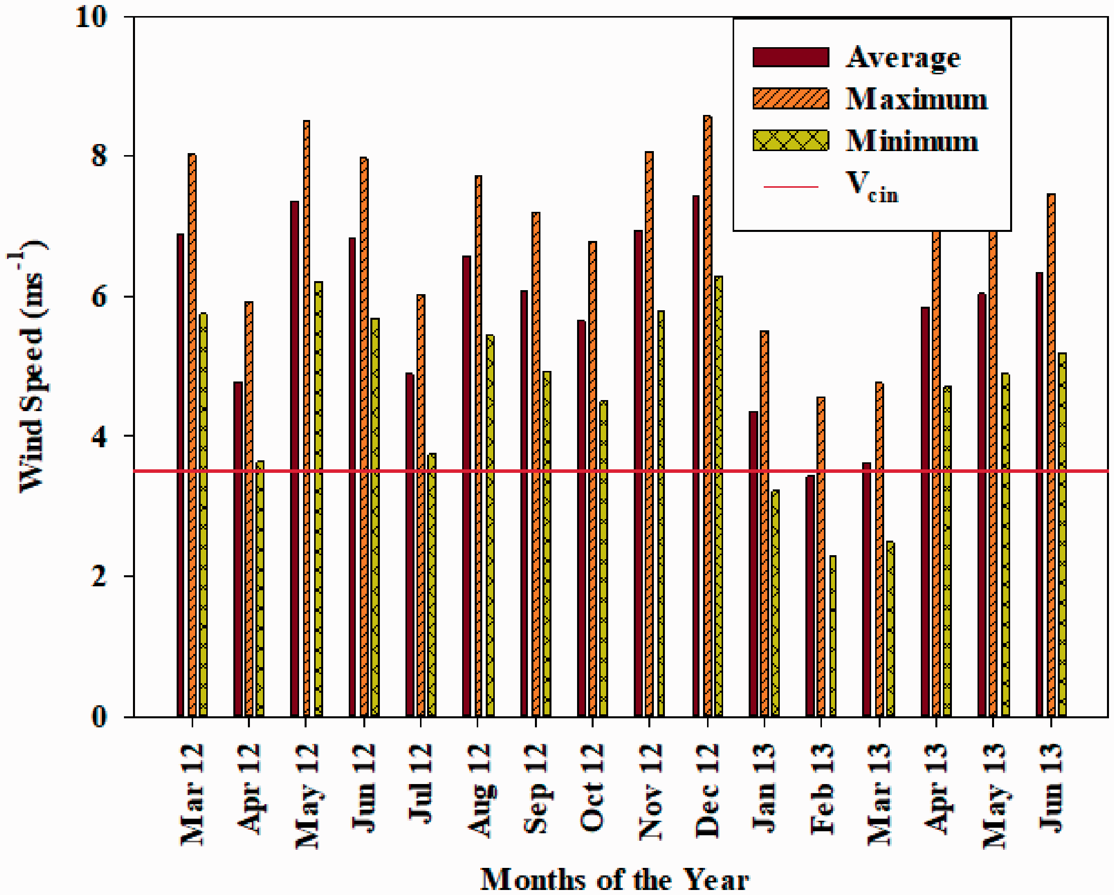
Average, maximum and minimum wind speed measured at 34 m a.g.l. (March 2012 to June 2013).

The maximum, minimum and average wind speeds at 34 m a.g.l were 6.97, 4.68 and 5.82 ms⁻¹ respectively. According to Brower (2012) the maximum and minimum wind speed values should be recorded at every interval as it plays a significant role in gust parameter determination which can have an effect on the suitability of the wind turbine. Months of January, February and March show least available wind for the turbine to harvest.

Turbulence intensity

The foremost effects of turbulence is the friction of the wind with the earth surface, and local variations of temperature in the atmosphere. Thus, the turbulence will depend on the type of topography and its environments. To measure the level of turbulence, the Turbulence intensity factor, TI, is used. It is generally defined for a time scale of 10 minutes.

T I = \frac{σ_{u}}{\bar{U}}

(17)

where

σ_{u}

the standard deviation and

\bar{U}

is the average wind speed over short period of time (ms⁻¹).

Daily turbulence intensities for every 10 minutes’ intervals were calculated. The mean daily turbulence intensity was also calculated as shown in Figure 5.

Figure 5.

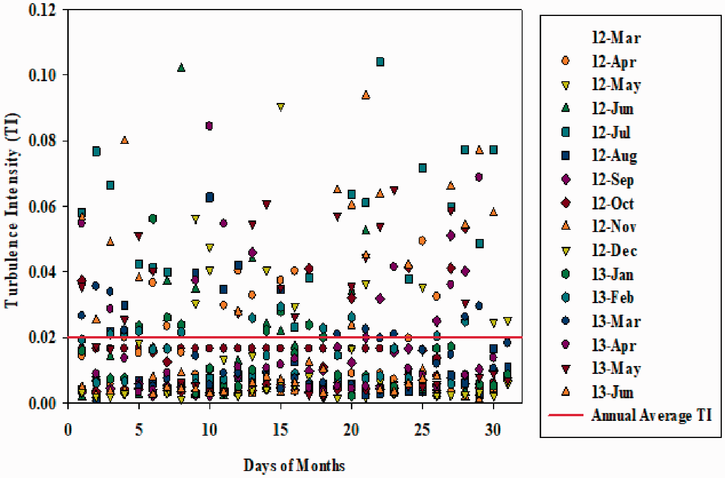
The diurnal average turbulence intensity on the same days of each month (March 2012 to June 2013) at 34 m a.g.l.

The annual average turbulent intensity is approximately 0.02 that is 2% therefore the wind at Nasawana is least turbulent. Around 70.3% of the time during each month the TI is less than the annual average TI as stated above. As evident from Figure 5, July 2012 recorded the highest Turbulence Intensity (TI) og 60%.

Wind speed frequency distributions

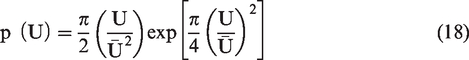
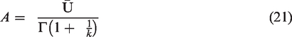
The probability that a wind speed lies within the operation range cut-in wind speed of 3.5 ms⁻¹ and cut-out wind speed of 25 ms⁻¹ of Vergnet 275 kW wind turbine is described by Rayleigh and Weibull Distributions. Rayleigh distribution is the simplest probability distribution since it uses one parameter, the mean wind speed to represent the wind distribution. The Rayleigh probability density function p(U), the probability of wind speed U is expressed as:

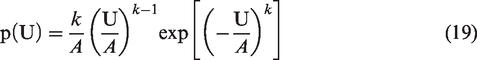
p (U) = \frac{π}{2} (\frac{U}{{\bar{U}}^{2}}) \exp [\frac{π}{4} {(\frac{U}{\bar{U}})}^{2}]

(18)

Weibull probability density depends on two variables, shape factor (k) and scale factor (A). k is a dimensional less factor which designates wind speed stability and is related to discrepancy of wind speed. The scale factor A is related to the mean wind speed, the higher the A value the higher the wind speed for a particular month. The Weibull distribution can be fitted to wind data time series by using the maximum likelihood method. Many application software including Wind Atlas Analysis and Applications (WAsP) use Weibull distribution described by

p (U) = \frac{k}{A} {(\frac{U}{A})}^{k - 1} \exp [{(- \frac{U}{A})}^{k}]

(19)

Both the parameters k and A can be approximated by the monthly mean wind speed (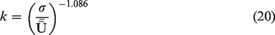 $U$ ) and the standard deviation (σ). The two factors are expressed by solving the following equations. For 1 ≤ k < 10, k is expressed as

k = {(\frac{σ}{\bar{\bar{U}}})}^{- 1.086}

(20)

The scale factor, A, is approximated as:

A = \frac{\bar{U}}{Γ (1 + \frac{1}{k})}

(21)

where Γ(x) is a gamma function of variable x

Γ (x) = \int_{0}^{\infty} x^{n - 1} e^{- x} d x

(22)

Hulio et al. (2019) using Weibull parameters comprehensively determined the wind potential and economics for Hawke’s bay, Pakistan.

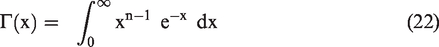
The probability that the wind speed was between 3.5 ms⁻¹ (cut-in) and 25 ms⁻¹ (cut-out) as estimated by Rayleigh and Weibull function were 75. 3% and 72.8% respectively. However, manual calculation yielded 72.7%. This explains that both distribution function adequately estimates the wind speed distribution.

The comparison (Figure 6) shows that Rayleigh distribution closely approximates the manual calculation and thus was chosen for further estimation.

Figure 6.

Relationship of the predicted Weibull and Rayleigh probability with the actual measured probability at 34 m a.g.l.

WAsP software analysis

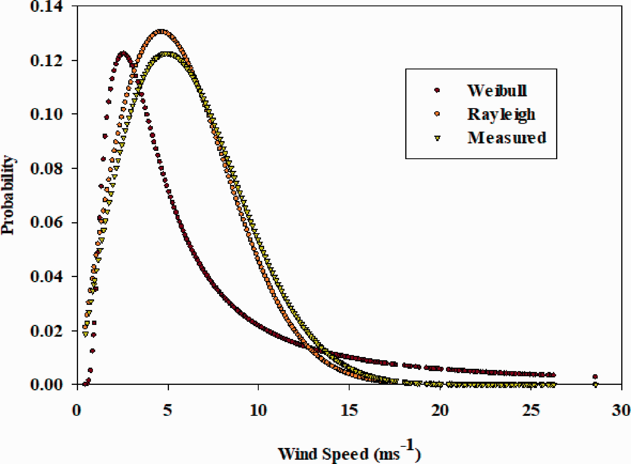
Wind power density (WPD) a measure of the power availability in the wind at a specific location or as an average over a longer period of time, indicates the potential of wind to generate electricity. The observed wind climate (OWC) report at a height of 34 m above the ground level (a.g.l) for Nasawana monitoring site specified that an average wind speed was 5.91 ms⁻¹ with an average power density of 206 Wm⁻² (Figure 7). The power density was > 100 Wm⁻² and hence could be considered as an average site for wind turbine installation.

Figure 7.

OWC report for Nasawana at 34 m a.g.l.

Researchers on wind power and energy production suggest that for most windy conditions the shape parameter (k) values range from 1.5–3.0 whereas scale factor (A) range from 3–8 ms⁻¹ (Fyrippis et al., 2010). The Nasawana site had comparable values (k = 2.42, A = 6.7 ms⁻¹). The result also suggested that around 40% of the time the wind is south eastly.

The forecast wind climate (Figure 8) shows the predicted wind speed distributions at 55 m a.g.l for each sector and its Weibull statistics.

Figure 8.

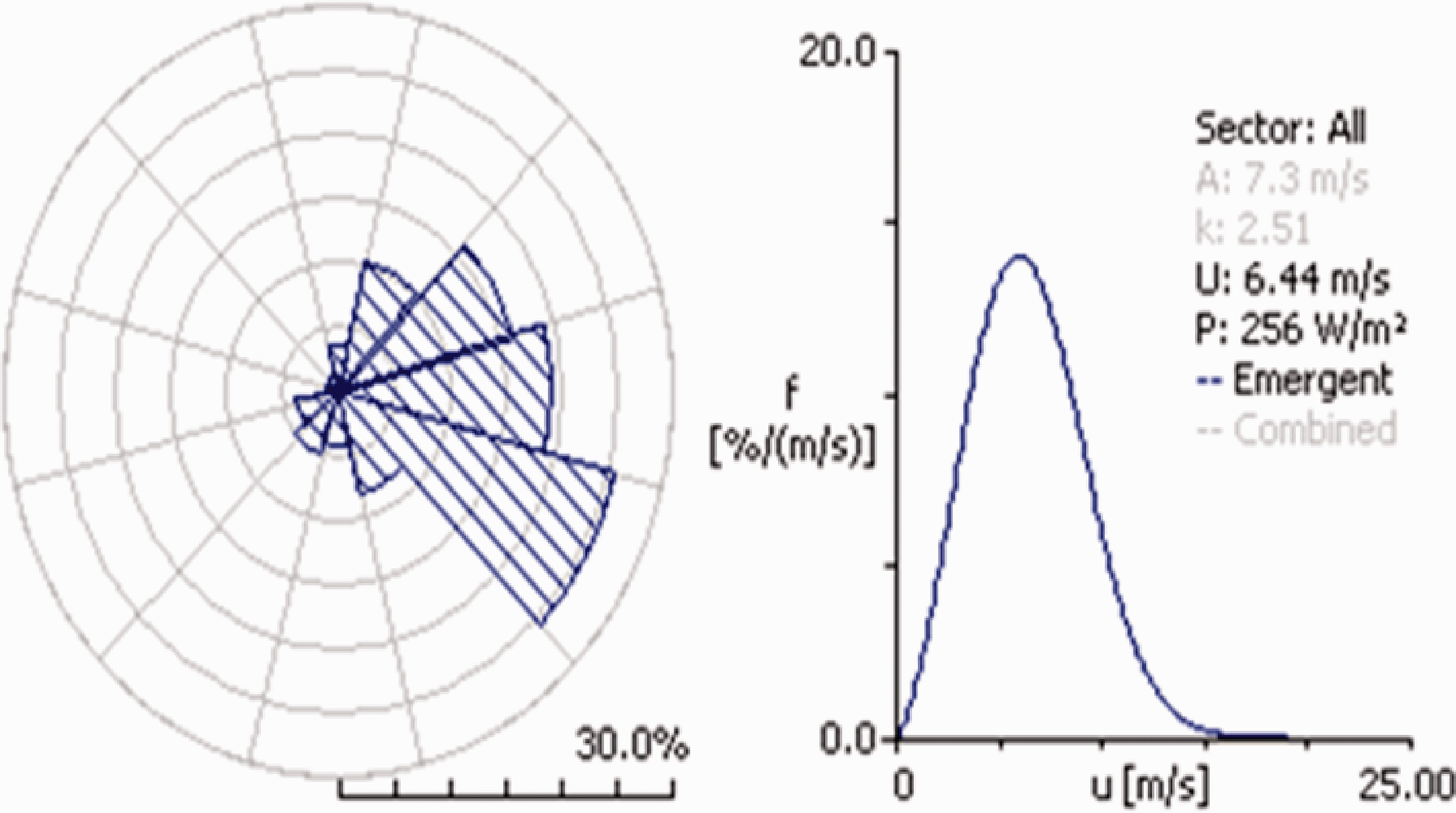
Wind Statistics at 55 m.

Wind speed and power characteristics have been studied widely and several researchers have reported the characteristic wind patterns and economics of wind farm. Baseer et al. (2015) studied several commercial wind turbines for Jubail industrial city reported that a 3.0 MW rated wind turbine was the most suitable at maximum power density of 168.46 Wm⁻².

The above results suggested that an average wind speed of 6.44 ms⁻¹ at 55 m a.g.l. However, the majority (≃ 30%) of the time, the wind was blowing from east. It also indicated the range of wind speed around the study site was between 3.63 and 11.22 ms⁻¹. At the measurement site the mean wind speed was approximately 5.82 ms⁻¹ at 34 m a.g.l. Rehman et al. (2020a) using 38 years of hourly mean wind speed data from seven locations reported that with decreasing latitude wind speed increases with lesser variation in wind direction. Manwell et al. (2010) stated that power density of 400 Wm⁻² can be considered as good site and greater than 700 Wm⁻² is a great site for wind turbine installation The power density at 55 m was greater than 250 Wm⁻² and this suggests that the site is an “average” site for a wind turbine for power generation.

WAsP predicted (Figure 9) a maximum of 1.45 GWh and a minimum of 0.113 GWh within the 25 km⁻². However, for the study site it estimated an AEP of 631.6 MWh. This suggests that the study site is a possible candidate site for a wind turbine installation.

Figure 9.

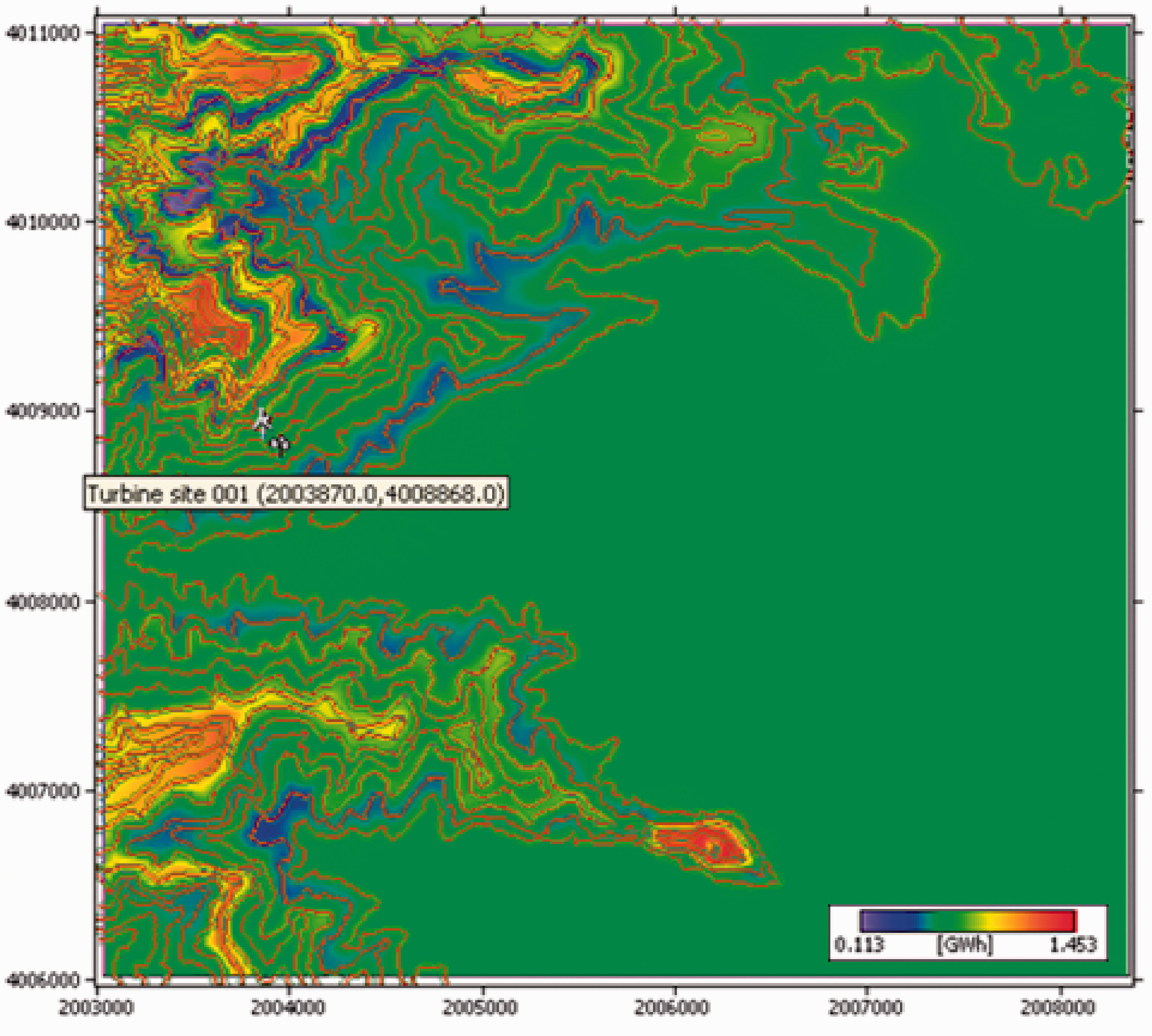
AEP at Nasawana.

The derived power curve (equation (23)) was obtained using curve fitting technique to manually calculate the AEP from the Vergnet 275 kW wind turbine (Gosai, 2014).

P (kW) = \frac{275}{[1 + \exp^{[\frac{- 1 (\bar{U} - 8.5)}{1.2}]}}

(23)

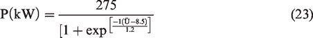
The empirical data for the Nasawana site was used to determine percentage error between the predicted and the manually calculated AEP values. It was necessary to compare the results of WAsP with manual calculations using the derived power curve to determine the accuracy of the software estimations. The result shows the difference in the two estimations. The difference in the value indicates the accuracy of the estimations at the anemometer site. The WAsP and manual calculation for AEP were 631.62 MWh and 595.29 MWh respectively with a difference of 36.33 MWh. Thus, the results suggests that WAsP over predicted the AEP and power density at the Nasawana site by 6.1%.

According to Acker and Chime (2011) using WAsP as the height of the wind data used for prediction increases higher than the monitoring hub height in this case from 34 m to 55 m, energy predicted by the software will contain more error due to derived shear calculation of WAsP Software.

The economic analysis of the system was determined to find the cost of energy, how long it would take to cover the initial investment, cost of one kWh of electricity, annual electricity return (R_A), Net Present Value (NPV), Benefit to Cost ratio (BCR), capital recovery factor (CF) and payback period (n). Using equations (1) to (14) above, Table 3 shows the economic parameters of 275 kW Vergnet wind turbine. The capital cost of Vergnet 275 kW wind turbine was estimated at $8,10,000 (based on the Butoni wind farm estimate). The real rate of discount was assumed as 3.2%, interest rate at 10%, inflation rate at 4% and escalation rate at 2.5%. Presently Energy Fiji Limited (EFL, 2018) buys electricity from IPP’s at FJD 0.27 per kWh and the electricity price is $0.35 per kWh. Based on the above assumptions the results obtained (Table 3) based on AEP estimated by WAsP.

Table 3.

Economics of a turbine installation at the Nasawana site.

Economic parameters		Vergnet 275 kWWAsP
Capital Cost	$	810,000
Cost of Turbine	$	55,080
Annual Energy Production	kWh	631,616
Capacity Factor	C_F	0.26
Annual Returns from Electricity Sales (B_A)	$	170,536
Net Present Value of Benefits (NPV) B_A	$	1,451,872
Annual O&M and land rent ( C_A)	$	32,400
Net Present Value (O&M and land rent (NPV) C_A	$	473,693
Net Present Value of the project (NPV)	$	609,472
Benefit Cost Ratio (BCR)		1.13
Payback period (n) years		6.59 ∼ 7
yearly cost of operation	$	64,185
Cost of kWh production	$	0.10
Internal Rate of Return (IRR)	%	16.21

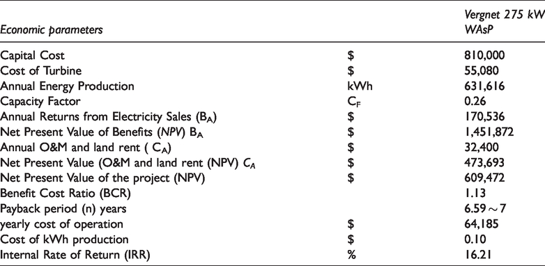
The WAsP result considered the surrounding terrains, shows BCR of 1.13, payback period (n) of 7 years and cost of energy as FJD 0.10/kWh. From the above calculations, it is clearly evident that there is adequate wind regime at the Nasawana site. Thus, Vergnet 275 kW installed at Nasawana shall produce sufficient energy to be economically feasible.

Conclusion

WAsP simulation results predicted the OWC with mean wind speed of 5.91 ms⁻¹ and a power density of 206 Wm⁻² at 34 m a.g.l. It also predicted a mean wind speed of 6.96 ms⁻¹ with power density of 256 Wm⁻² at 55 m a.g.l. A 275 kW Vergnet turbine at the Nasawana village is expected to produce 631.62 MWh annually at FJD 0.10/kWh with a payback period of 7 years. This generation cost compared against EFL’S purchase price of FJD 0.27/kWh, shows that investing in wind power generation at Nasawana is economically viable.

Footnotes

Declaration of conflicting interests

The author(s) declared no potential conflicts of interest with respect to the research, authorship, and/or publication of this article.

Funding

The author(s) received no financial support for the research, authorship, and/or publication of this article.

ORCID iD

Krishnam Nair

References

Acker

Chime

(2011) Wind Modeling Using WindPro and WAsP Software. Flagstaff: Sustainable Energy Solution lab, Mechanical Engineering Department, Northern Arizona University.

Baseer

Meyer

Alam

, et al. (2015) Wind speed and power characteristics for Jubail industrial city, Saudi Arabia. Renewable and Sustainable Energy Reviews 52: 1193–1204.

Baseer

Rehman

Meyer

, et al. (2017) GIS-based site suitability analysis for wind farm development in Saudi Arabia. Energy 141: 1166–1176.

Bassyouni

Gutub Saud

Javaid

, et al. (2015) Assessment and analysis of wind power resource using Weibull parameters. Energy Exploration & Exploitation 33(1): 105–122.

Brower

(2012) Wind Resource Assessment: A Practical Guide to Developing a Wind Project. New Jersey: John Wiley & Sons Inc.

Clean Development Mechanism Investors (2012) Guide Republic of Fiji. Available at: https://theredddesk.org/sites/default/files/fiji_clean_development_mechanism_cdm_policy_guidelines.pdf (accessed 29 June 2020).

Energy Fiji Limited (2018) Annual Report. Available at: http://www.parliament.gov.fj/wp-content/uploads/2019/06/Energy-Fiji-Limited-2018-Annual-Report.pdf (accessed 21 October 2020).

Fiji Bureau of Statistics Releases Census Results (2017) Available at www.fiji.gov.fj/Media-Centre/News/Fiji-Bureau-of-Statistics-Releases-2017-Census-Res (accessed July 2020).

Fyrippis

Axaopoulos

Panayiotou

(2010) Wind energy potential assessment in Naxos Island, Greece. Applied Energy 87(2): 577–586.

10.

Gosai

(2014) Wind Energy Potential and Electricity Generation at Rokavukavu, Rakiraki in Fiji. Unpublished MSc Thesis, The University of the South Pacific, Suva, Fiji.

11.

Hulio

Jiang

Rehman

(2019) Techno-economic assessment of wind power potential of Hawke’s Bay using Weibull parameter: A review. Energy Strategy Reviews 26: 100375.

12.

Khadem

Hussain

(2006) A pre-feasibility study of wind resources in Kutubdia Island, Bangladesh. Renewable Energy 31(14): 2329–2341.

13.

Kumar

Nair

(2012) Wind characteristics and energy potentials at Wainiyaku Taveuni, Fiji. Management of Environmental Quality: An International Journal 23(3): 300–308.

14.

Kumar

Nair

(2013) Wind power potential at Benau, Savusavu, Vanua Levu, Fiji. International Journal of Energy, Information and Communications 4: 51–62.

15.

Kumar

Prasad

(2010) Examining wind quality and wind power prospects on Fiji islands. Renewable Energy 35(2): 536–540.

16.

Manwell

McGowan

Rogers

(2010) Wind Energy Explained: Theory Design and Application. 2nd ed. Hoboken: John Wiley & Sons Inc.

17.

Pacific Energy Country Profiles (2016) Pacific Energy Conference, New Zealand Ministry of Foreign Affairs & Trade. Available at: www.mfat.govt.nz/assets/Aid-Prog-docs/Renewable-Energy/Country-Energy-Profiles-FINAL-web-version.pdf (accessed 7 July 2020).

18.

Rafique

Rehman

Alam

, et al. (2018) Feasibility of a 100 MW installed capacity wind farm for different climatic conditions. Energy Exploration & Exploitation 11(8): 2147.

19.

Rehman

Mohandes

Alhems

(2018) Wind speed and power characteristics using LiDAR anemometer based measurements. Sustainable Energy Technologies and Assessments 27: 46–62.

20.

Rehman

Natarajan

Mohandes

, et al. (2020a) Latitudinal wind power resource assessment along coastal areas of Tamil Nadu, India. Faculty of Mechanical Engineering, Belgrade 48: 566–575.

21.

Rehman

Natarajan

Vasudevan

, et al. (2020b) Assessment of wind energy potential across varying topographical features of Tamil Nadu, India. Energy Exploration & Exploitation 38(1): 175–200.

22.

REN (2018) 21 Renewables Global Status Report, REN21 Secretariat. Paris: REN.

23.

Shata

ASA

Hanitsch

(2006) Evaluation of wind energy potential and electricity generation on the Coast of Mediterranean sea in Egypt. Renewable Energy 31(8): 1183–1202.

24.

Shoaib

Siddiqui

Rehman

, et al. (2019) Assessment of wind energy potential using wind energy conversion system. Journal of Cleaner Production 216: 346–360.

25.

The World Bank Data (2020) Available at: https://data.worldbank.org/indicator/EG.ELC.ACCS.ZS?locations=FJ (accessed 29 June 2020).

26.

Troen I and Petersen EL (1989) European Wind Atlas. Roskilde: Risø National Laboratory, ISBN 87:550-1482-8. Available at: https://www.wasp.dk/news/2015/08/european-wind-atlas-now-available-for-download?id=f999e21a-4243-428c-a878-f2268113221c (accessed 21 October 2020).

Potential of wind energy resources around Nasawana village in Nabouwalu,Vanua Levu,Fiji

Abstract

Keywords

Introduction

Current developments of wind in the pacific

South pacific wind climatology

Wind resource estimate using WAsP

Wind energy economics

Description of the study site

Methodology

Instrumentation, data recording and acquisition

Result and discussion

Nasawana village wind data analysis

Daily wind speed analysis

Turbulence intensity

Wind speed frequency distributions

WAsP software analysis

Conclusion

Footnotes

Declaration of conflicting interests

Funding

ORCID iD

References