Sage Journals: Discover world-class research

Abstract

Application of Weibull distribution in a generalized way to estimate wind potential cannot always be advisable. The novelty of this work is to estimate wind potential using Normal probability density function. A comparison of five probability distributions namely Normal, Gamma, Chi-Squared, Weibull, and Rayleigh was done using three performance evaluation criteria. Four years (2015–2018) hourly wind data at 50 m height at five stations near the coastline of Pakistan was used. It was found that normal distribution gives the best fit at each of these stations and against each evaluation criterion followed by Weibull distribution while Rayleigh distribution gives the poorest fit. Further energy generation by fifteen turbine models was calculated and GE 45.7 was found the best in terms of amount of energy generation and capacity factors while Vestas V42 shows the worst. However, GE/1.5 SL is the most economical while Vestas V63 is the least. Among five locations, Shahbandar is the best potential site while Manora is the least.

Keywords

Continuous probability density functions comparison of various probability distributions wind potential estimation techno-economic feasibility analysis coastal area of Pakistan

Introduction

Continuous probability distributions are widely used to model various phenomenon in science, engineering, technology, and sociology, etc. (Silveira et al., 2019). Such distributions help a lot in solving real life problems e.g. analysis of material failure estimation, estimation of rainfall, prediction of water level, and various resource assessments (Sumair et al., 2020e; Seguro and Lambert, 2000); among resource assessments, one of the attractive field is wind resource assessment (WRA). As wind is an extremely random phenomenon, its magnitude varies diurnally, monthly, seasonally, and annually. Therefore, there is a dire need to model this widely varying random phenomenon before its exploitation at a particular area.

Wind power production potential at Hyderabad was estimated (Gul et al., 2019) using Weibull distribution. Two-years meteorological data (at 10 m height) was used to investigate the wind characteristics. Wind pattern were found to be steady based on monthly and seasonal variation analysis. Moreover, it was found that a wind speed of about 6 m/s can be observed throughout the year. Average annual wind power density and energy density were found to be 255 W/m² and 2245 kWh/m², respectively. Also, commercially available wind turbines could produces wind energy at $0.019 to $0.032 per unit of energy.

Analysis of incorporation of windmills in Karachi has been conducted and presented in (Aman et al., 2013). Four years wind data was used which was measured at five different hub heights of 10, 30, 50, 75, and 100 m was utilized. A case study was performed to show the effect of windmills installation, which showed that there would be an approximate savings of about 1678 MWh of energy provided that 50% of residential consumers make use of windmills.

Exploration of wind energy at Keti Bandar was made with the purpose of finding its feasibility to contribute towards the electrical energy generation of country (Ullah et al., 2010) using one-year wind data. Site was recognized with good wind potential. Hence, the site was shown to be a good candidate of wind energy utilization for both small scale and stand-alone systems. To model wind data, Weibull distribution has widely been used throughout the world (Andrade et al., 2014; Arslan et al., 2014; Bagiorgas et al., 2012, 2016; Baseer et al., 2017; Bassyouni et al., 2015; Safari and Gasore, 2010; Shami et al., 2016; Sumair et al., 2020c, 2020d; Khahro et al., 2014a, 2014b).

Many researchers have suggested that no single distribution should be used for wind potential estimation but a comparison of various probability distributions should be made to identify the best fit prior to the estimation of wind potential (Sumair et al., 2020e; Kollu et al., 2012; Lollchund et al., 2014; Pobočíková et al., 2017; Rajapaksha and Perera, 2016). Hence, it is neither advisable nor rational to always apply Weibull distribution for wind potential estimation without a comparison of various distributions.

The novelty of this work is to compare five probability distributions as no such comparison has been conducted in literature prior to estimate the wind potential using the best fit found. Moreover, current work estimates the wind potential using Normal distribution (rather than using Weibull distribution) which has not been used so far for WRA. As coastal area of Pakistan has been reported to possess about 43 GW of wind potential (Shoaib et al., 2017) but site-specific wind potential for many locations still needs to be investigated. Therefore, this work is concerned about the exploration of wind potential of five such locations situated in the coastal area of Pakistan as shown in Figure 1.

Figure 1.

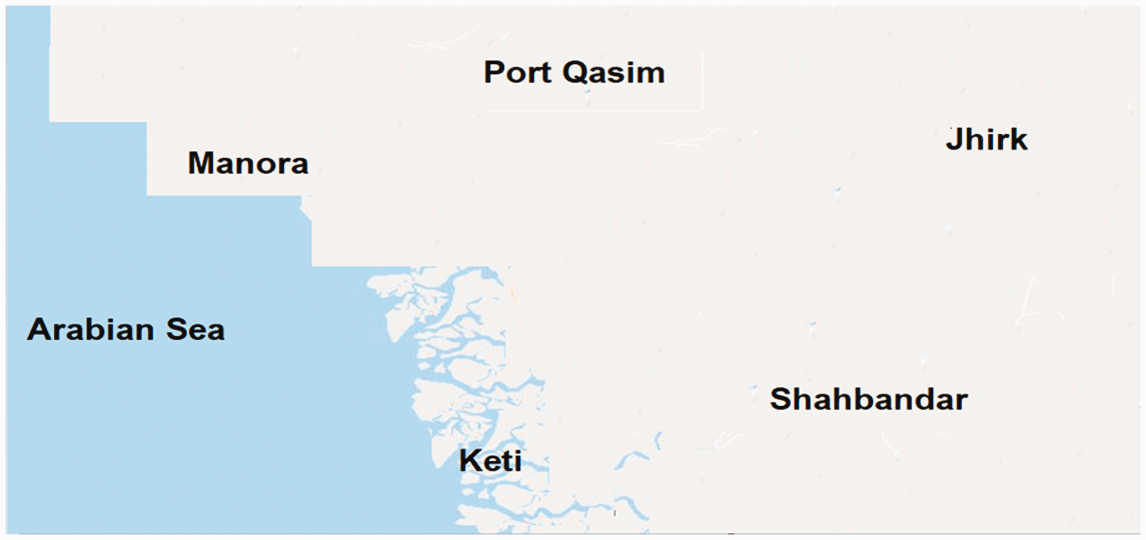
Geographical map showing five stations in the coastal area of Pakistan.

Materials and methods

A comparison among five probability distributions i.e. Normal, Gamma, Chi-Squared, Weibull, and Rayleigh distribution were carried out using four years hourly recorded wind data. Wind data was collected at 50 m height at five stations namely Jhirk, Keti, Manora, Port Qasim, and Shahbandar by Pakistan Metrological Department (PMD). Parameters of these distributions were estimated using Moment Method. Comparison was made using three performance evaluation criteria. Each distribution was ranked against each evaluation criteria followed by an overall ranking. Detailed effectiveness of wind energy production by turbines at selected sites was carried out. Finally, the results were validated using historical data approach.

Following five probability distributions were used in the foregoing study.

Normal distribution

The most widely used distribution throughout the entire statistical field is Normal or Gaussian probability distribution with two variables as µ and σ is given as follows (Ross, 2009, 2014; Walpole et al., 2011)

f (V) = \frac{1}{σ \sqrt{2 π}} e^{- \frac{1}{2 σ^{2}} {(V - μ)}^{2}}

(1)

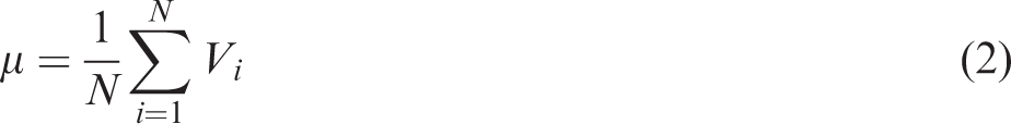
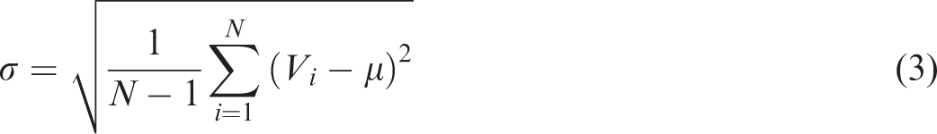
µ and σ are given by equations (2) and (3), respectively

μ = \frac{1}{N} \sum_{i = 1}^{N} V_{i}

(2)

σ = \sqrt{\frac{1}{N - 1} \sum_{i = 1}^{N} {(V_{i} - µ)}^{2}}

(3)

N=Total Observations

Gamma distribution

Although Normal distribution is the most widely used distributions, some other distributions are also required to model some phenomenon. One such distribution is Gamma distribution, given as follows (Pobočíková et al., 2017; Ross, 2014; Walpole et al., 2011)

f (V) = \frac{1}{β^{α} Γ (α)} V^{(α - 1)} e^{- V / β}

(4)

α and β are gamma distribution parameters and Γ(α) is an important mathematical function, presented in following equation (5)

Γ (α) = \int_{0}^{\infty} z^{α - 1} e^{- z} d z

(5)

Method of moment (MOM) estimates of Gamma distribution are given as follows

μ = α β

(6)

σ^{2} = α β^{2}

(7)

Chi square distribution

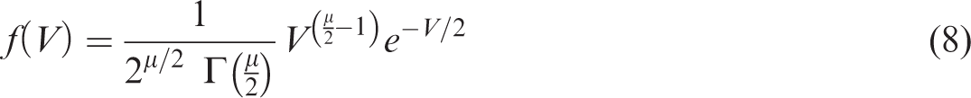
As Gamma distribution is a generalized distribution; its special case is Chi Square distribution with α = µ/2 and β = 2 (Walpole et al., 2011). With these modifications, equation (4) becomes

f (V) = \frac{1}{2^{μ / 2} Γ (\frac{μ}{2})} V^{(\frac{μ}{2} - 1)} e^{- V / 2}

(8)

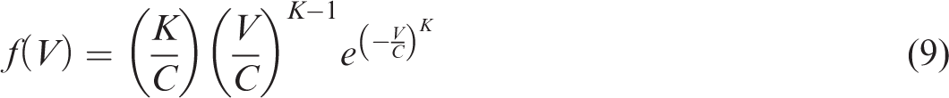
Weibull distribution

Two parameters of this distribution are represented by K and C, and its density function is given below (Aized et al., 2019; Bagiorgas et al., 2012; Khahro et al., 2014a, 2014b; Shoaib et al., 2017; Sumair et al., 2020a; 2020b).

f (V) = (\frac{K}{C}) {(\frac{V}{C})}^{K - 1} e^{{(- \frac{V}{C})}^{K}}

(9)

C = \frac{µ}{Γ (1 + \frac{1}{K})}

(10)

σ = C {[Γ (1 + \frac{2}{K}) - Γ^{2} (1 + \frac{2}{K})]}^{0.5}

(11)

Rayleigh distribution

Just as Chi Square distribution is deduced from Gamma distribution; so is the case of Rayleigh distribution deduction with Weibull distribution with K = 2 and C = µ (Khahro et al., 2014a, 2014b). Thus, equation (9) assumes the following form

f (V) = (\frac{2}{μ}) (\frac{V}{μ}) e^{{(- \frac{V}{μ})}^{2}}

(12)

Performance comparison of distributions

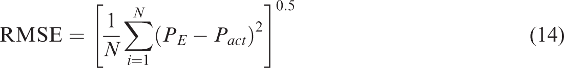
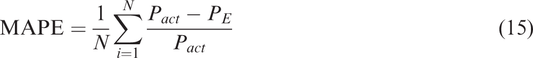
Well-known and widely used statistical parameters have been applied to compare the performance of these distributions. These parameters i.e. R², RMSE, and MAPE have been calculated using equations (13) to (15), respectively

R^{2} = \frac{\sum_{i = 1}^{N} {(P_{E} - Z)}^{2} - \sum_{i = 1}^{N} {(P_{act} - Z)}^{2}}{\sum_{i = 1}^{N} {(P_{E} - Z)}^{2}}

(13)

RMSE = {[\frac{1}{N} \sum_{i = 1}^{N} ({P_{E} - P_{act})}^{2}]}^{0.5}

(14)

MAPE = \frac{1}{N} \sum_{i = 1}^{N} |\frac{P_{act} - P_{E}}{P_{act}}|

(15)

P_act is the actual probability while P_E is estimated probability from probability distribution.

Wind power density

Wind power density is calculated using following relationship

P_{D} (V) = \frac{1}{2} ρ V^{3}

(16)

However, while modeling the wind data using probability density functions, a more realistic approach to find power density is to use equation (17) (Manwell et al., 2010).

P_{D} = \int_{0}^{\infty} P_{D} (V) \times f (V) d V

(17)

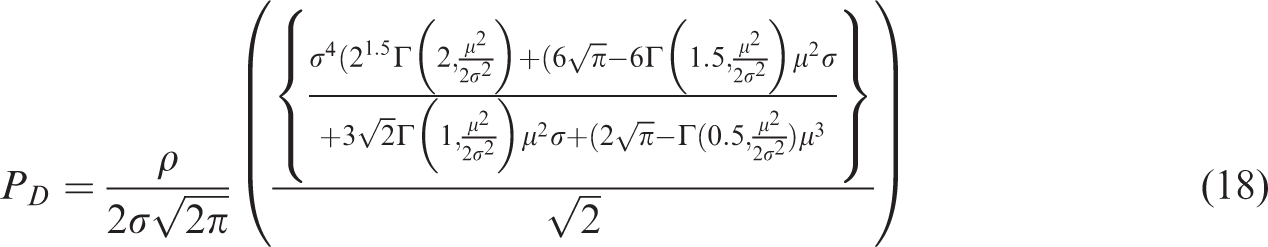
Applying normal probability density function in equation (17), we get the following relationship for wind power density estimation

P_{D} = \frac{ρ}{2 σ \sqrt{2 π}} (\frac{\{\frac{σ^{4} (2^{1.5} Γ (2, \frac{μ^{2}}{2 σ^{2}}) + (6 \sqrt{π} - 6 Γ (1.5, \frac{μ^{2}}{2 σ^{2}}) μ^{2} σ}{+ 3 \sqrt{2} Γ (1, \frac{μ^{2}}{2 σ^{2}}) μ^{2} σ + (2 \sqrt{π} - Γ (0.5, \frac{μ^{2}}{2 σ^{2}}) μ^{3}}\}}{\sqrt{2}})

(18)

where Γ (α,y) is incomplete gamma function defined by equation (19)

Γ (a, y) = \int_{y}^{\infty} z^{a - 1} e^{- z} d z

(19)

Energy Generation Effectiveness Analysis

Theoretically, wind carries a certain amount of potential but this whole potential can never be exploited because of the limitations imposed by turbine and energy extraction system's inefficiencies. Therefore, to take into account these facts, power produced by a typical extraction system is evaluated by equation (20) (Manwell et al., 2010).

P_{W T} = \frac{1}{2} ρ A C_{p} η V^{3}

(20)

C_p in equation (20) is power coefficient, given by Betz criterion (16/27) (Khahro et al., 2014b) and η is drive train effcicnecy (assumed 100%). As there are always fluctuations in wind speeds and the occurrence with which a certain wind blows, hence a more realistic approach is to evaluate average power using following equation (21)

\bar{P_{W T}} = \int_{0}^{\infty} P_{W T} d f (V)

(21)

Once the power is evaluated, energy, AEP, can simply be evaluated by multiplying it with time T over which energy generation is under consideration

AEP = \bar{P_{W T}} T

(22)

As mentioned above that any energy or power extraction system has its own inherent inefficiencies which cause the reduction of power production, there is a need to describe how well a system or turbine is performing relative to its maximum possible capacity. One such parameter used to describe this performance is capacity factor (CF), given in equation (23)

C F = \frac{P_{actual}}{P_{rated}}

(23)

However, economic feasibility of a power project cannot be determined from CF only. A turbine having low CF is not necessarily unfeasible. Thus to evalutae the economic feasibility, other parameters such as given in equation (24) and (25) below, are required to be calculated.

Payback period (PP) = \frac{Total cost o f project}{cost o f energy produced per year}

(24)

PP is the time period (usually measured in years) in which a project recovers its total cost. And

C = \frac{Net present value (NPV)}{E_{p}}

(25)

NPV is algebraic difference between two quantities; input to any project and output form that project, both in terms of money. NPV can be evaluated with the help of equation (26) with I as investment, j as rate of interest, m is a constant which is taken as 0.3I and t as approximate lifetime of power extraction system

NPV = I (1 + m (\frac{{(1 + j)}^{t} - 1}{j {(1 + j)}^{t}}))

(26)

Results and discussions

Comparison of probability distributions

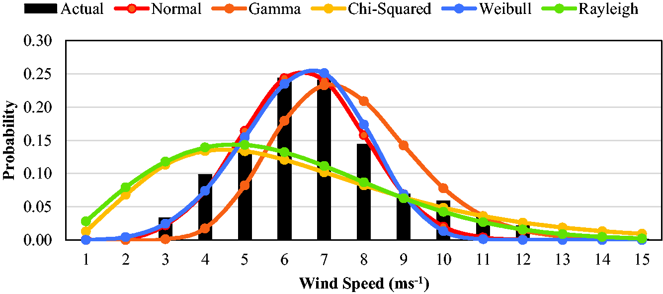
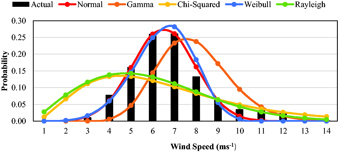
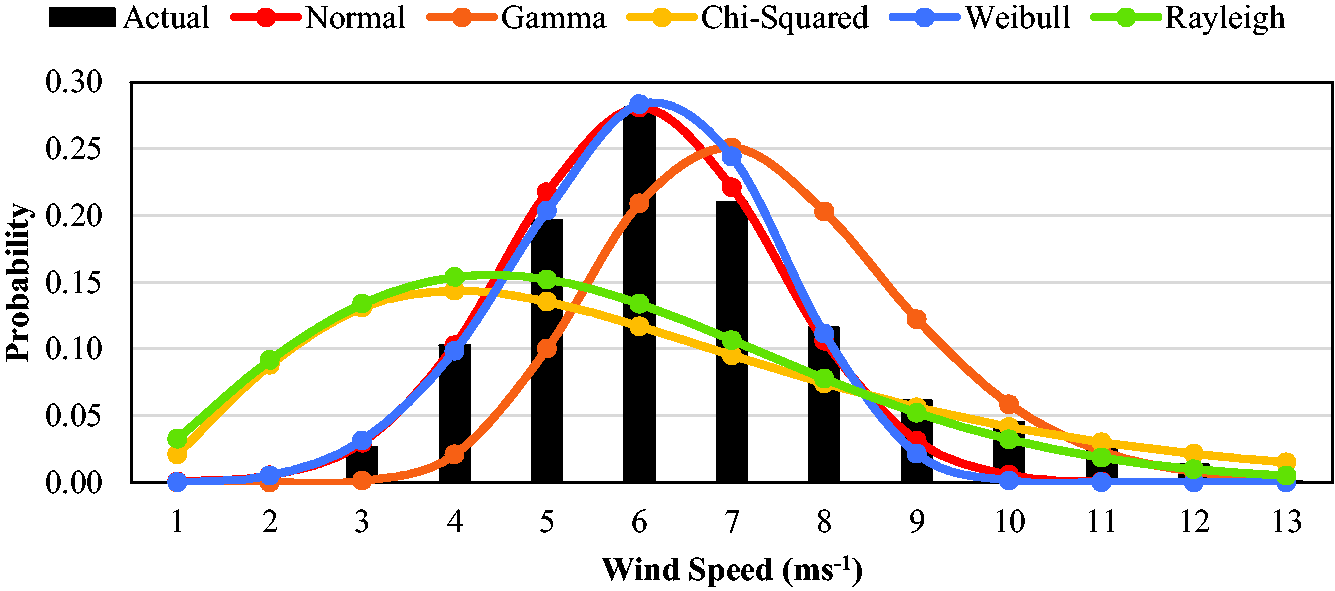
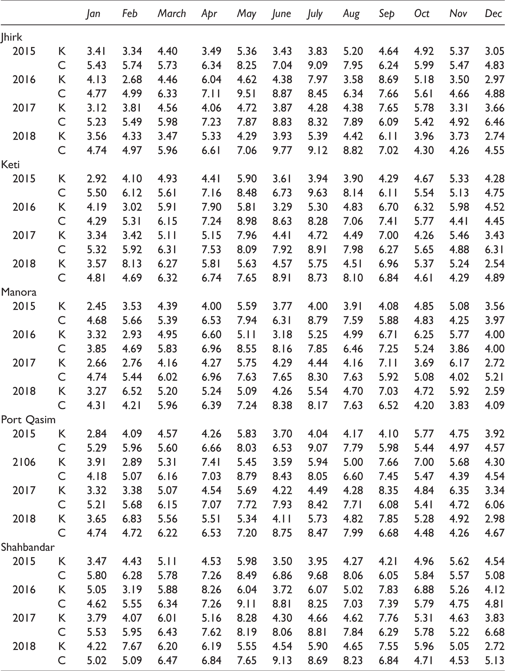
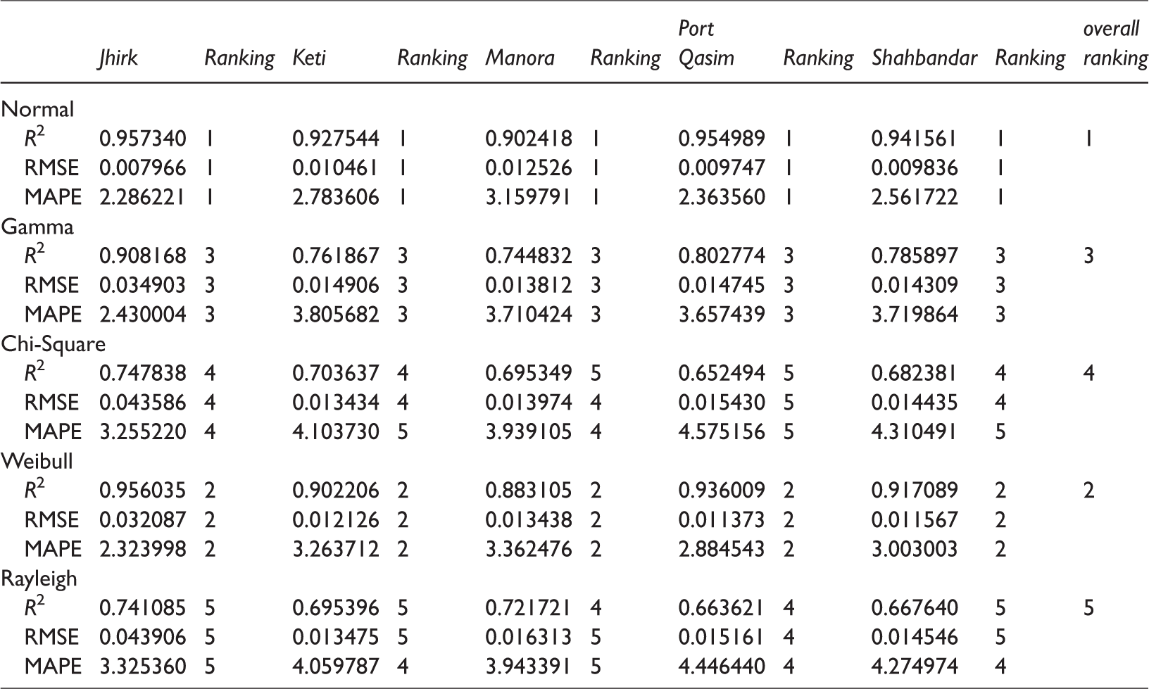
As there are certain parameters or variables needed to completely define any distribution and to apply it for probability determination, these required parameters were estimated and separately written in Tables 1 to 3. As the purpose of applying more than one distributions was to compare them before actually making a wind potential estimation, therefore, efficiency of these distributions were analyzed and compared, as written in Table 4. Each distribution has been ranked (at a scale of 1–5 with 1 as the best performance and 5 as the least) against each evaluation criteria for each station and then an overall ranking has been done. Comparison of performance of all these five distributions shows that, for each of the studied station, it is not the Weibull distribution which can evaluate wind potential with the highest accuracy but is the Normal distribution. However, Weibull distribution has been found to generate second highest degree of accuracy. Whereas the performance of Rayleigh distribution is the worst with Gamma and Chi-Square distributions lying in between these extremes with Gamma distribution giving superior performance than Chi square. Graphical representation of these distributions has been shown in Figures 2 to 6, respectively.

Figure 2.

Performance assessment of all distributions at Jhirk station.

Figure 3.

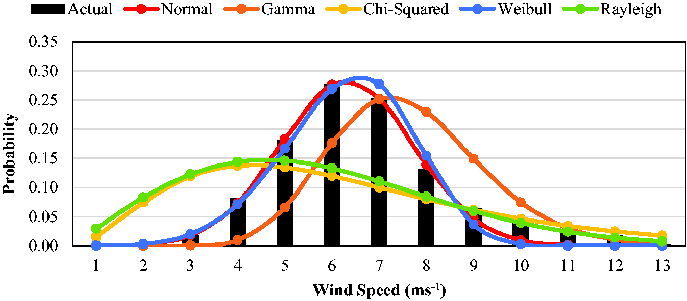
Performance assessment of all distributions at Keti station.

Figure 4.

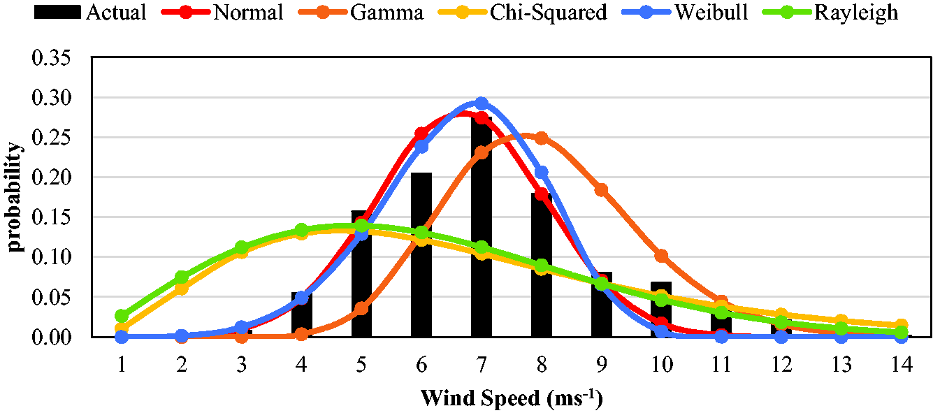
Performance assessment of all distributions at Manora station.

Figure 5.

Performance assessment of all distributions at Port Qasim station.

Figure 6.

Performance assessment of all distributions at Shahbandar station.

Table 1.

Monthly average values of normal distribution parameters at each station.

		Jan	Feb	March	Apr	May	June	July	Aug	Sep	Oct	Nov	Dec
Jhirk
2015	μ	4.88	5.15	5.22	5.71	7.61	6.33	8.22	7.32	5.70	5.49	5.04	4.32
	σ	1.57	1.70	1.34	1.81	1.63	2.04	2.39	1.62	1.40	1.27	1.08	1.55
2016	μ	4.33	4.44	5.77	6.60	8.69	8.08	7.96	5.71	7.24	5.16	4.19	4.35
	σ	1.18	1.78	1.47	1.26	2.14	2.09	1.17	1.76	0.99	1.14	1.32	1.60
2017	μ	4.68	4.96	5.46	6.56	7.20	7.99	7.57	7.19	5.72	5.01	4.41	5.83
	σ	1.64	1.45	1.36	1.81	1.73	2.31	1.99	1.86	0.88	1.00	1.47	1.77
2018	μ	4.27	4.53	5.36	6.10	6.42	8.85	8.41	8.04	6.52	3.89	3.85	4.05
	σ	1.33	1.17	1.71	1.32	1.68	2.52	1.80	2.06	1.23	1.10	1.15	1.60
Keti
2015	μ	4.91	5.55	5.14	6.53	7.86	6.07	8.72	7.37	5.56	5.07	4.73	4.32
	σ	1.82	1.52	1.19	1.66	1.54	1.86	2.48	2.11	1.46	1.23	1.01	1.14
2016	μ	3.90	4.74	5.70	6.81	8.32	7.74	7.63	6.47	6.91	5.37	4.09	4.06
	σ	1.04	1.71	1.12	1.02	1.66	2.59	1.65	1.52	1.20	0.99	0.79	1.02
2017	μ	4.78	5.32	5.80	6.92	7.61	7.22	8.16	7.28	5.86	5.14	4.51	5.67
	σ	1.57	1.72	1.29	1.54	1.13	1.84	1.97	1.84	0.97	1.36	0.94	1.83
2018	μ	4.34	4.42	5.88	6.24	7.07	8.13	8.08	7.40	6.39	4.25	3.95	4.34
	σ	1.35	0.64	1.09	1.24	1.45	2.02	1.63	1.86	1.07	0.90	0.86	1.83
Manora
2015	μ	4.15	5.10	4.91	5.92	7.34	5.70	7.97	6.87	5.33	4.43	3.90	3.58
	σ	1.81	1.60	1.27	1.65	1.51	1.68	2.22	1.97	1.47	1.04	0.88	1.11
2016	μ	3.45	4.19	5.35	6.49	7.86	7.31	7.23	5.93	6.77	4.87	3.57	3.62
	σ	1.15	1.56	1.23	1.15	1.75	2.52	1.57	1.36	1.18	0.90	0.71	0.89
2017	μ	4.21	4.84	5.47	6.33	7.06	6.96	7.57	6.93	5.54	4.58	3.73	4.64
	σ	1.71	1.90	1.48	1.67	1.42	1.82	1.93	1.87	0.91	1.38	0.70	1.84
2018	μ	3.86	3.92	5.48	5.88	6.65	7.62	7.54	6.98	6.10	3.84	3.55	3.63
	σ	1.30	0.70	1.20	1.28	1.49	2.01	1.57	1.69	1.01	0.93	0.69	1.51
Port Qasim
2015	μ	4.71	5.41	5.12	6.06	7.43	5.89	8.23	7.08	5.43	5.03	4.55	4.13
	σ	1.79	1.48	1.26	1.60	1.47	1.77	2.28	1.91	1.49	1.00	1.09	1.18
2016	μ	3.79	4.52	5.67	6.60	8.11	7.59	7.46	6.06	7.00	5.12	4.06	4.14
	σ	1.08	1.69	1.22	1.04	1.71	2.35	1.45	1.38	1.07	0.86	0.82	1.08
2017	μ	4.67	5.11	5.65	6.46	7.14	7.21	7.68	7.02	5.74	4.96	4.39	5.44
	σ	1.55	1.66	1.28	1.60	1.44	1.92	1.93	1.85	0.80	1.17	0.81	1.79
2018	μ	4.28	4.41	5.74	6.03	6.64	7.94	7.84	7.32	6.29	4.12	3.91	4.17
	σ	1.30	0.76	1.19	1.26	1.43	2.17	1.57	1.73	0.94	0.90	0.91	1.53
Shahbandar
2015	μ	5.22	5.73	5.31	6.63	7.88	6.17	8.77	7.33	5.50	5.36	5.15	4.63
	σ	1.66	1.46	1.19	1.65	1.52	1.95	2.49	1.94	1.47	1.24	1.06	1.15
2016	μ	4.25	4.97	5.88	6.85	8.45	7.96	7.66	6.45	6.96	5.41	4.38	4.36
	σ	0.96	1.71	1.15	0.97	1.61	2.38	1.46	1.47	1.04	0.92	0.95	1.19
2017	μ	5.00	5.40	5.96	7.01	7.73	7.34	8.05	7.17	5.92	5.33	4.77	6.04
	σ	1.47	1.49	1.14	1.56	1.09	1.92	1.95	1.75	0.89	1.15	1.17	1.76
2018	μ	4.57	4.79	6.02	6.36	7.06	8.34	8.06	7.52	6.43	4.37	4.16	4.57
	σ	1.22	0.73	1.12	1.18	1.46	2.07	1.57	1.83	1.00	0.84	0.94	1.81

Table 2.

Monthly average values of gamma distribution parameters at each station.

		Jan	Feb	March	Apr	May	June	July	Aug	Sep	Oct	Nov	Dec
Jhirk
2015	β	0.51	0.56	0.35	0.57	0.35	0.66	0.69	0.36	0.34	0.29	0.23	0.56
	α	9.61	9.18	15.13	9.96	21.72	9.63	11.85	20.49	16.67	18.69	21.81	7.78
2016	β	0.32	0.72	0.37	0.24	0.53	0.54	0.17	0.54	0.13	0.25	0.42	0.59
	α	13.55	6.18	15.52	27.41	16.52	14.98	46.33	10.53	53.69	20.39	10.03	7.42
2017	β	0.57	0.42	0.34	0.50	0.42	0.67	0.52	0.48	0.13	0.20	0.49	0.54
	α	8.18	11.74	16.15	13.09	17.24	11.99	14.52	15.01	42.57	25.14	8.94	10.86
2018	β	0.41	0.30	0.54	0.28	0.44	0.72	0.38	0.53	0.23	0.31	0.34	0.63
	α	10.37	14.91	9.85	21.49	14.61	12.34	21.91	15.22	28.05	12.51	11.24	6.43
Keti
2015	β	0.68	0.42	0.27	0.42	0.30	0.57	0.71	0.61	0.38	0.30	0.22	0.30
	α	7.24	13.33	18.72	15.38	25.97	10.65	12.37	12.14	14.58	16.90	21.82	14.50
2016	β	0.28	0.62	0.22	0.15	0.33	0.87	0.35	0.36	0.21	0.18	0.15	0.26
	α	13.92	7.66	26.00	44.79	25.22	8.94	21.51	18.01	33.27	29.58	26.60	15.88
2017	β	0.52	0.55	0.29	0.34	0.17	0.47	0.47	0.46	0.16	0.36	0.20	0.59
	α	9.26	9.60	20.05	20.33	45.44	15.37	17.20	15.71	36.32	14.37	22.86	9.64
2018	β	0.42	0.09	0.20	0.25	0.30	0.50	0.33	0.47	0.18	0.19	0.19	0.77
	α	10.39	47.42	29.18	25.18	23.71	16.20	24.74	15.82	35.96	22.11	21.03	5.63
Manora
2015	β	0.79	0.50	0.33	0.46	0.31	0.50	0.62	0.56	0.41	0.24	0.20	0.35
	α	5.24	10.15	15.06	12.79	23.47	11.51	12.86	12.18	13.16	18.09	19.88	10.35
2016	β	0.38	0.58	0.28	0.20	0.39	0.87	0.34	0.31	0.21	0.17	0.14	0.22
	α	9.03	7.23	18.81	31.95	20.07	8.40	21.25	19.14	32.94	29.51	24.97	16.76
2017	β	0.69	0.74	0.40	0.44	0.29	0.48	0.49	0.51	0.15	0.42	0.13	0.73
	α	6.09	6.52	13.68	14.44	24.74	14.59	15.36	13.70	36.94	10.94	28.72	6.35
2018	β	0.44	0.13	0.26	0.28	0.33	0.53	0.33	0.41	0.17	0.22	0.13	0.63
	α	8.79	31.20	20.81	21.17	19.90	14.39	23.04	17.07	36.18	17.20	26.31	5.80
Port Qasim
2015	β	0.68	0.41	0.31	0.42	0.29	0.53	0.63	0.51	0.41	0.20	0.26	0.34
	α	6.89	13.31	16.43	14.36	25.64	11.02	12.97	13.77	13.34	25.11	17.35	12.28
2016	β	0.31	0.63	0.26	0.17	0.36	0.73	0.28	0.32	0.16	0.14	0.17	0.28
	α	12.22	7.14	21.45	39.92	22.50	10.44	26.63	19.14	42.70	35.76	24.36	14.62
2017	β	0.51	0.54	0.29	0.40	0.29	0.51	0.48	0.49	0.11	0.28	0.15	0.59
	α	9.11	9.41	19.61	16.20	24.46	14.08	15.85	14.46	51.04	18.00	29.70	9.22
2018	β	0.40	0.13	0.25	0.26	0.31	0.59	0.32	0.41	0.14	0.19	0.21	0.56
	α	10.77	34.03	23.40	23.01	21.62	13.40	24.79	17.88	44.86	21.19	18.58	7.46
Shahbandar
2015	β	0.53	0.37	0.27	0.41	0.29	0.62	0.71	0.51	0.39	0.28	0.22	0.29
	α	9.86	15.40	19.87	16.06	26.95	10.02	12.42	14.34	13.97	18.82	23.80	16.11
2016	β	0.22	0.59	0.23	0.14	0.31	0.71	0.28	0.34	0.16	0.16	0.21	0.32
	α	19.47	8.47	25.99	50.11	27.43	11.18	27.70	19.25	44.73	34.57	21.02	13.44
2017	β	0.43	0.41	0.22	0.35	0.15	0.50	0.47	0.43	0.13	0.25	0.28	0.51
	α	11.61	13.12	27.17	20.23	50.37	14.55	17.01	16.71	43.92	21.41	16.77	11.84
2018	β	0.33	0.11	0.21	0.22	0.30	0.52	0.31	0.45	0.15	0.16	0.21	0.72
	α	14.03	42.85	29.02	28.91	23.28	16.15	26.23	16.89	41.50	26.76	19.49	6.37

Table 3.

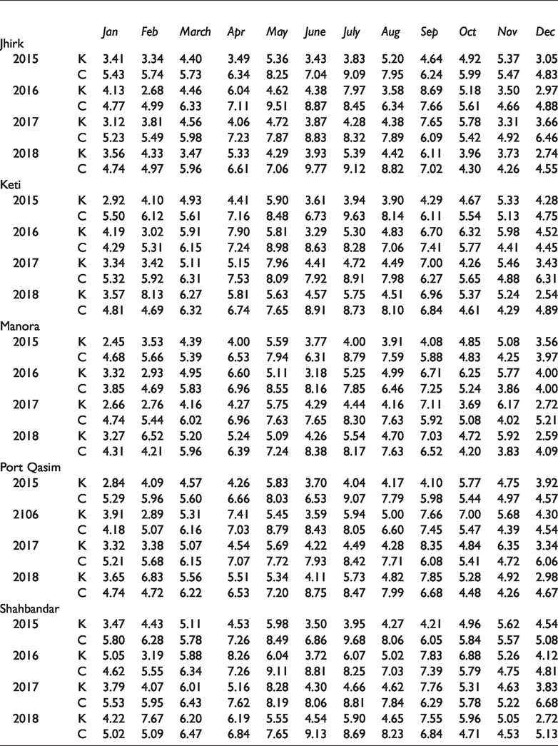
Monthly average values of Weibull parameters at each station.

		Jan	Feb	March	Apr	May	June	July	Aug	Sep	Oct	Nov	Dec
Jhirk
2015	K	3.41	3.34	4.40	3.49	5.36	3.43	3.83	5.20	4.64	4.92	5.37	3.05
	C	5.43	5.74	5.73	6.34	8.25	7.04	9.09	7.95	6.24	5.99	5.47	4.83
2016	K	4.13	2.68	4.46	6.04	4.62	4.38	7.97	3.58	8.69	5.18	3.50	2.97
	C	4.77	4.99	6.33	7.11	9.51	8.87	8.45	6.34	7.66	5.61	4.66	4.88
2017	K	3.12	3.81	4.56	4.06	4.72	3.87	4.28	4.38	7.65	5.78	3.31	3.66
	C	5.23	5.49	5.98	7.23	7.87	8.83	8.32	7.89	6.09	5.42	4.92	6.46
2018	K	3.56	4.33	3.47	5.33	4.29	3.93	5.39	4.42	6.11	3.96	3.73	2.74
	C	4.74	4.97	5.96	6.61	7.06	9.77	9.12	8.82	7.02	4.30	4.26	4.55
Keti
2015	K	2.92	4.10	4.93	4.41	5.90	3.61	3.94	3.90	4.29	4.67	5.33	4.28
	C	5.50	6.12	5.61	7.16	8.48	6.73	9.63	8.14	6.11	5.54	5.13	4.75
2016	K	4.19	3.02	5.91	7.90	5.81	3.29	5.30	4.83	6.70	6.32	5.98	4.52
	C	4.29	5.31	6.15	7.24	8.98	8.63	8.28	7.06	7.41	5.77	4.41	4.45
2017	K	3.34	3.42	5.11	5.15	7.96	4.41	4.72	4.49	7.00	4.26	5.46	3.43
	C	5.32	5.92	6.31	7.53	8.09	7.92	8.91	7.98	6.27	5.65	4.88	6.31
2018	K	3.57	8.13	6.27	5.81	5.63	4.57	5.75	4.51	6.96	5.37	5.24	2.54
	C	4.81	4.69	6.32	6.74	7.65	8.91	8.73	8.10	6.84	4.61	4.29	4.89
Manora
2015	K	2.45	3.53	4.39	4.00	5.59	3.77	4.00	3.91	4.08	4.85	5.08	3.56
	C	4.68	5.66	5.39	6.53	7.94	6.31	8.79	7.59	5.88	4.83	4.25	3.97
2016	K	3.32	2.93	4.95	6.60	5.11	3.18	5.25	4.99	6.71	6.25	5.77	4.00
	C	3.85	4.69	5.83	6.96	8.55	8.16	7.85	6.46	7.25	5.24	3.86	4.00
2017	K	2.66	2.76	4.16	4.27	5.75	4.29	4.44	4.16	7.11	3.69	6.17	2.72
	C	4.74	5.44	6.02	6.96	7.63	7.65	8.30	7.63	5.92	5.08	4.02	5.21
2018	K	3.27	6.52	5.20	5.24	5.09	4.26	5.54	4.70	7.03	4.72	5.92	2.59
	C	4.31	4.21	5.96	6.39	7.24	8.38	8.17	7.63	6.52	4.20	3.83	4.09
Port Qasim
2015	K	2.84	4.09	4.57	4.26	5.83	3.70	4.04	4.17	4.10	5.77	4.75	3.92
	C	5.29	5.96	5.60	6.66	8.03	6.53	9.07	7.79	5.98	5.44	4.97	4.57
2106	K	3.91	2.89	5.31	7.41	5.45	3.59	5.94	5.00	7.66	7.00	5.68	4.30
	C	4.18	5.07	6.16	7.03	8.79	8.43	8.05	6.60	7.45	5.47	4.39	4.54
2017	K	3.32	3.38	5.07	4.54	5.69	4.22	4.49	4.28	8.35	4.84	6.35	3.34
	C	5.21	5.68	6.15	7.07	7.72	7.93	8.42	7.71	6.08	5.41	4.72	6.06
2018	K	3.65	6.83	5.56	5.51	5.34	4.11	5.73	4.82	7.85	5.28	4.92	2.98
	C	4.74	4.72	6.22	6.53	7.20	8.75	8.47	7.99	6.68	4.48	4.26	4.67
Shahbandar
2015	K	3.47	4.43	5.11	4.53	5.98	3.50	3.95	4.27	4.21	4.96	5.62	4.54
	C	5.80	6.28	5.78	7.26	8.49	6.86	9.68	8.06	6.05	5.84	5.57	5.08
2016	K	5.05	3.19	5.88	8.26	6.04	3.72	6.07	5.02	7.83	6.88	5.26	4.12
	C	4.62	5.55	6.34	7.26	9.11	8.81	8.25	7.03	7.39	5.79	4.75	4.81
2017	K	3.79	4.07	6.01	5.16	8.28	4.30	4.66	4.62	7.76	5.31	4.63	3.83
	C	5.53	5.95	6.43	7.62	8.19	8.06	8.81	7.84	6.29	5.78	5.22	6.68
2018	K	4.22	7.67	6.20	6.19	5.55	4.54	5.90	4.65	7.55	5.96	5.05	2.72
	C	5.02	5.09	6.47	6.84	7.65	9.13	8.69	8.23	6.84	4.71	4.53	5.13

Table 4.

Comparison of five probability distributions based on R², RMSE and MAPE.

	Jhirk	Ranking	Keti	Ranking	Manora	Ranking	Port Qasim	Ranking	Shahbandar	Ranking	overall ranking
Normal
R²	0.957340	1	0.927544	1	0.902418	1	0.954989	1	0.941561	1	1
RMSE	0.007966	1	0.010461	1	0.012526	1	0.009747	1	0.009836	1
MAPE	2.286221	1	2.783606	1	3.159791	1	2.363560	1	2.561722	1
Gamma
R²	0.908168	3	0.761867	3	0.744832	3	0.802774	3	0.785897	3	3
RMSE	0.034903	3	0.014906	3	0.013812	3	0.014745	3	0.014309	3
MAPE	2.430004	3	3.805682	3	3.710424	3	3.657439	3	3.719864	3
Chi-Square
R²	0.747838	4	0.703637	4	0.695349	5	0.652494	5	0.682381	4	4
RMSE	0.043586	4	0.013434	4	0.013974	4	0.015430	5	0.014435	4
MAPE	3.255220	4	4.103730	5	3.939105	4	4.575156	5	4.310491	5
Weibull
R²	0.956035	2	0.902206	2	0.883105	2	0.936009	2	0.917089	2	2
RMSE	0.032087	2	0.012126	2	0.013438	2	0.011373	2	0.011567	2
MAPE	2.323998	2	3.263712	2	3.362476	2	2.884543	2	3.003003	2
Rayleigh
R²	0.741085	5	0.695396	5	0.721721	4	0.663621	4	0.667640	5	5
RMSE	0.043906	5	0.013475	5	0.016313	5	0.015161	4	0.014546	5
MAPE	3.325360	5	4.059787	4	3.943391	5	4.446440	4	4.274974	4

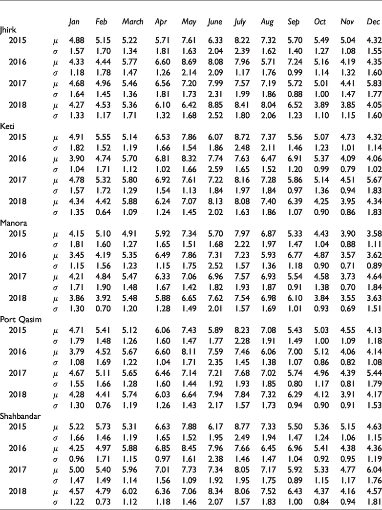
Monthly and seasonal variation in wind speed and wind power density

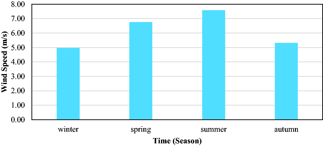
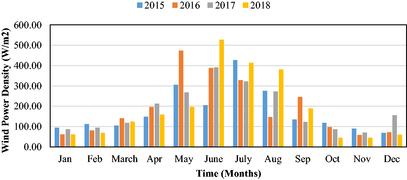
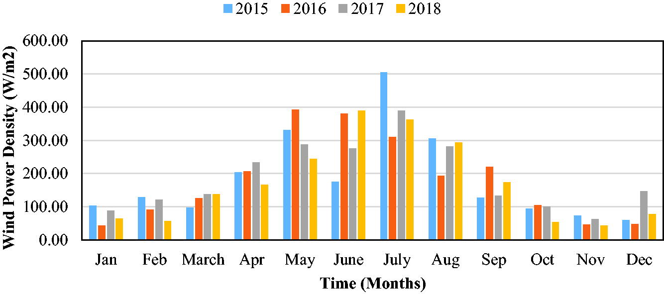
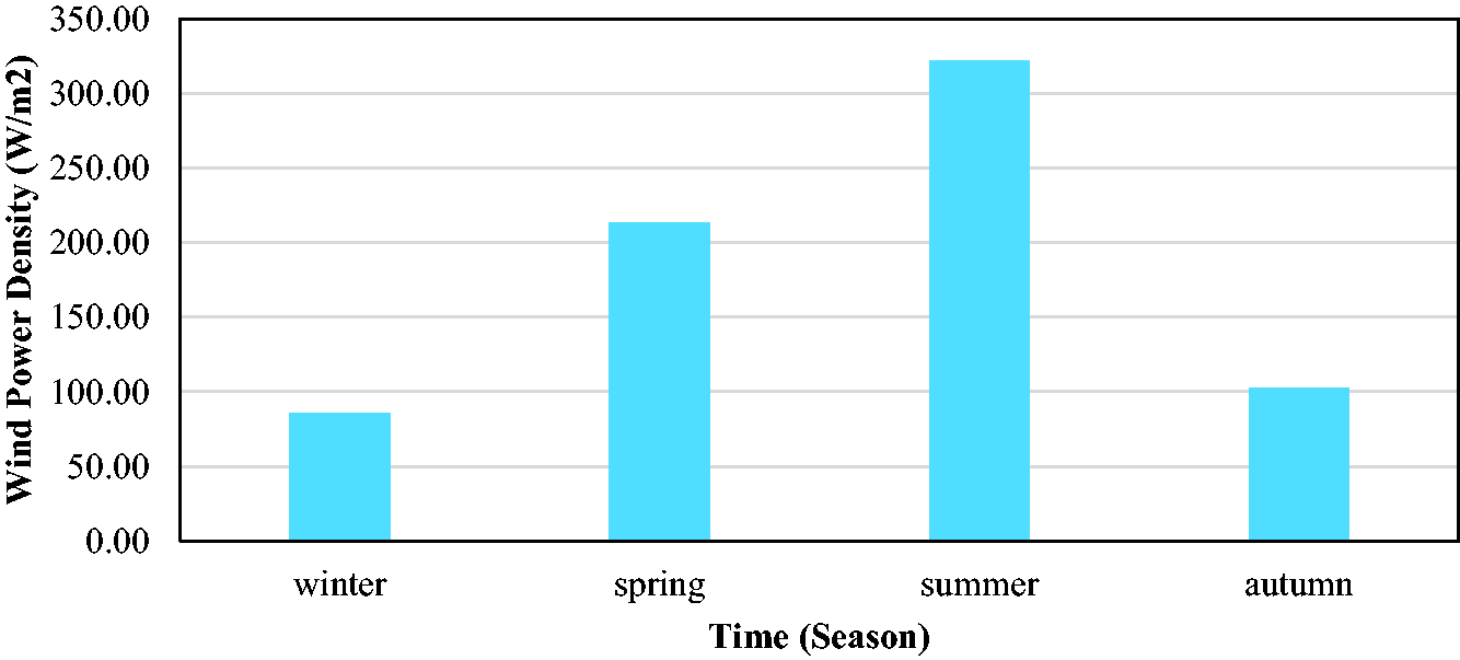
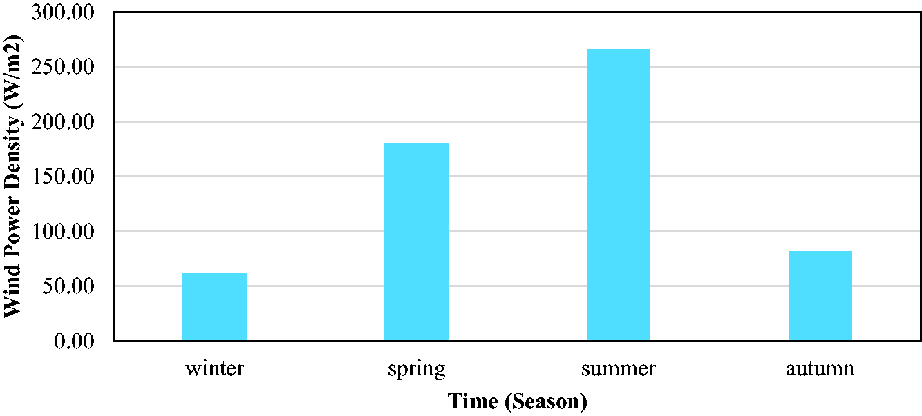
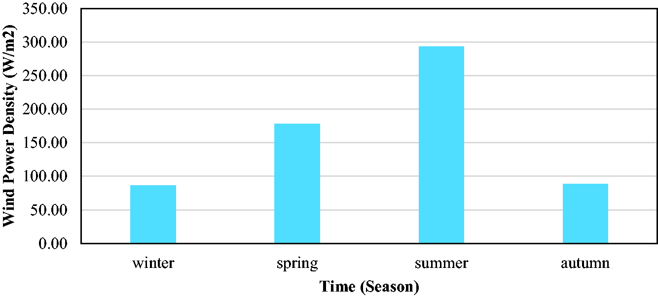
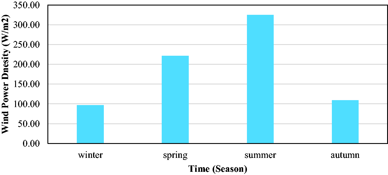
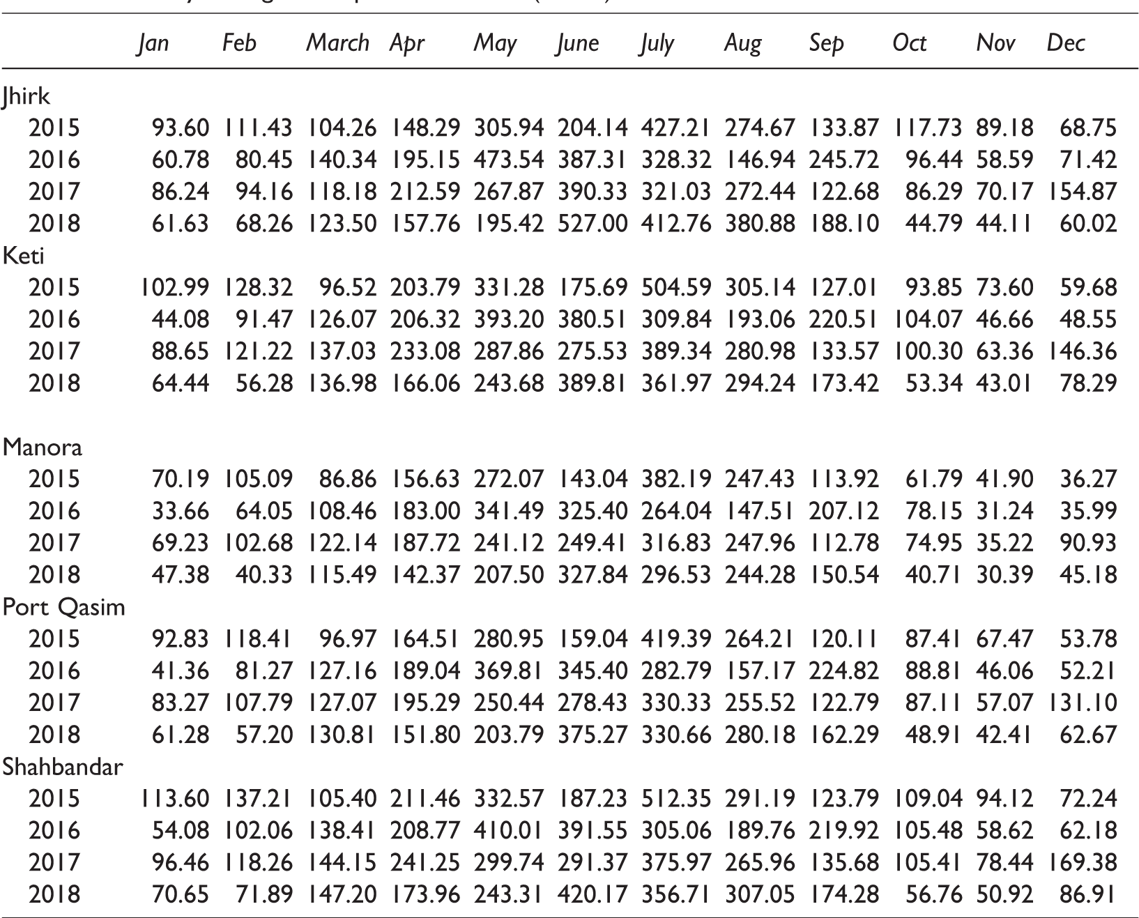
Figures 7 to 16 represent the variation observed in wind speeds on monthly and seasonal basis at all investigated locations. Analysis shows that wind blows with maximum speed in July and with minimum speed in January at all locations. Moreover, comparison of overall mean wind speed is depicted in Figure 17, which shows that Shahbandar has the highest mean wind speed while Manora has the lowest among all investigated locations with mean values of 6.15 and 5.52 m/s, respectively. Similarly, monthly and seasonal variation in wind power density has been shown in Figures 18 to 27 at all investigated locations as listed in Table 5. Analysis shows that maximum wind power density is observed in summer (July) and minimum in winter (January). Moreover, comparison of four years average values of wind power densities at all locations has been shown in Figure 28, which shows that Shahbandar has the highest value of wind power density while Manora has the lowest with values of 187.87 and 147.44 W/m², respectively.

Figure 7.

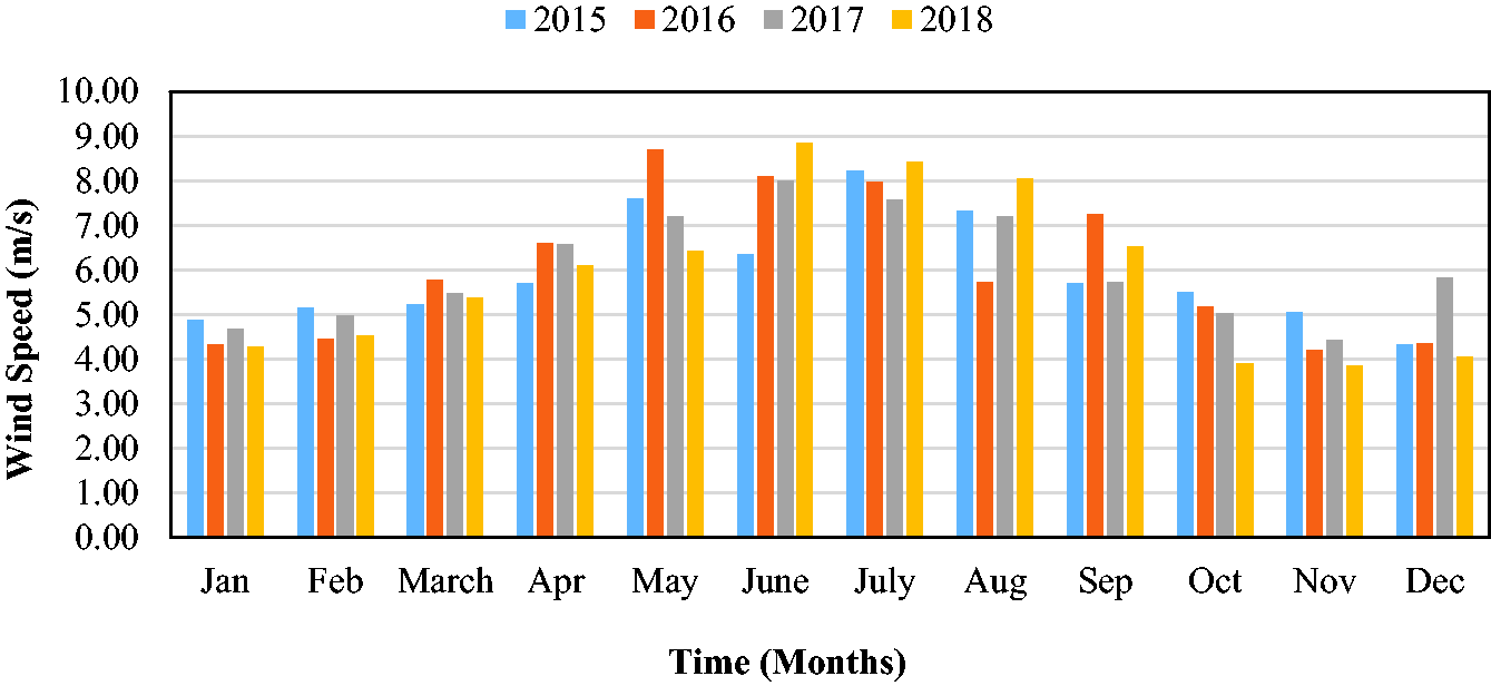
Variation observed in wind speed at Jhirk on monthly basis.

Figure 8.

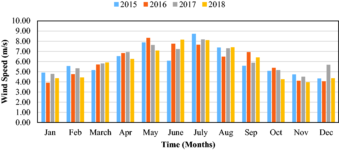
Variation observed in wind speed at Keti on monthly basis.

Figure 9.

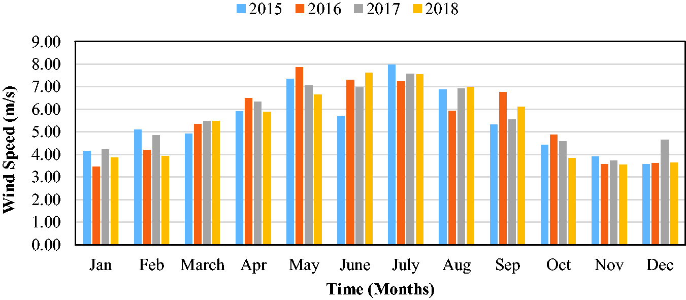
Variation observed in wind speed at Manora on monthly basis.

Figure 10.

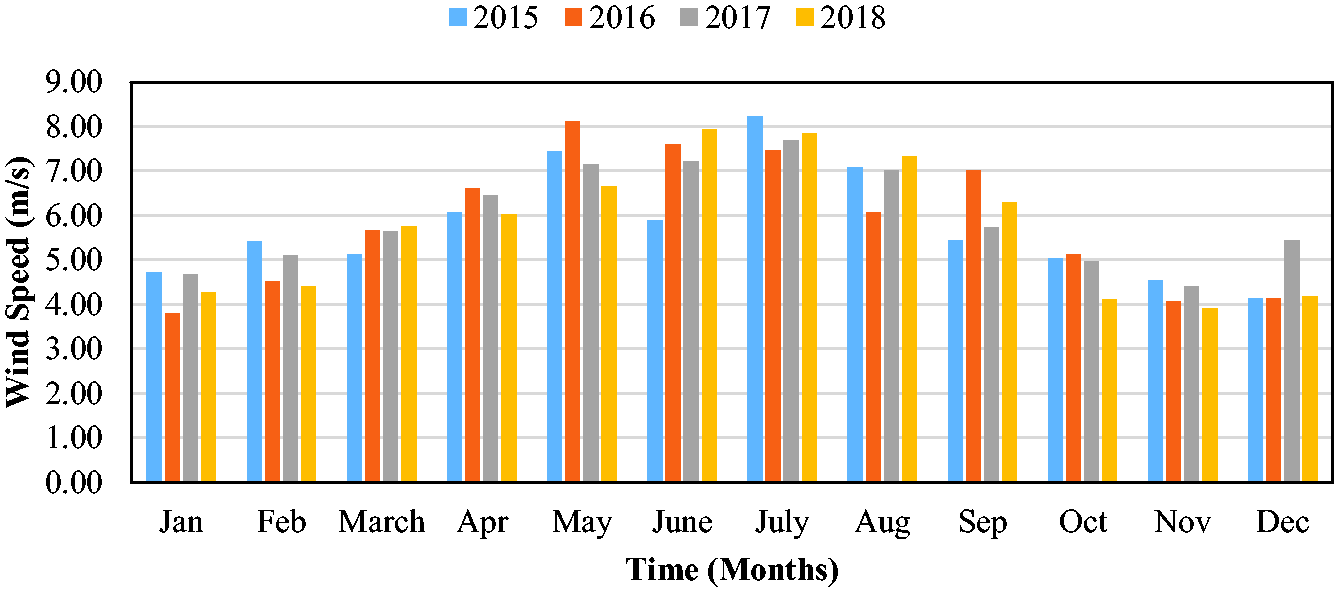
Variation observed in wind speed at Port Qasim on monthly basis.

Figure 11.

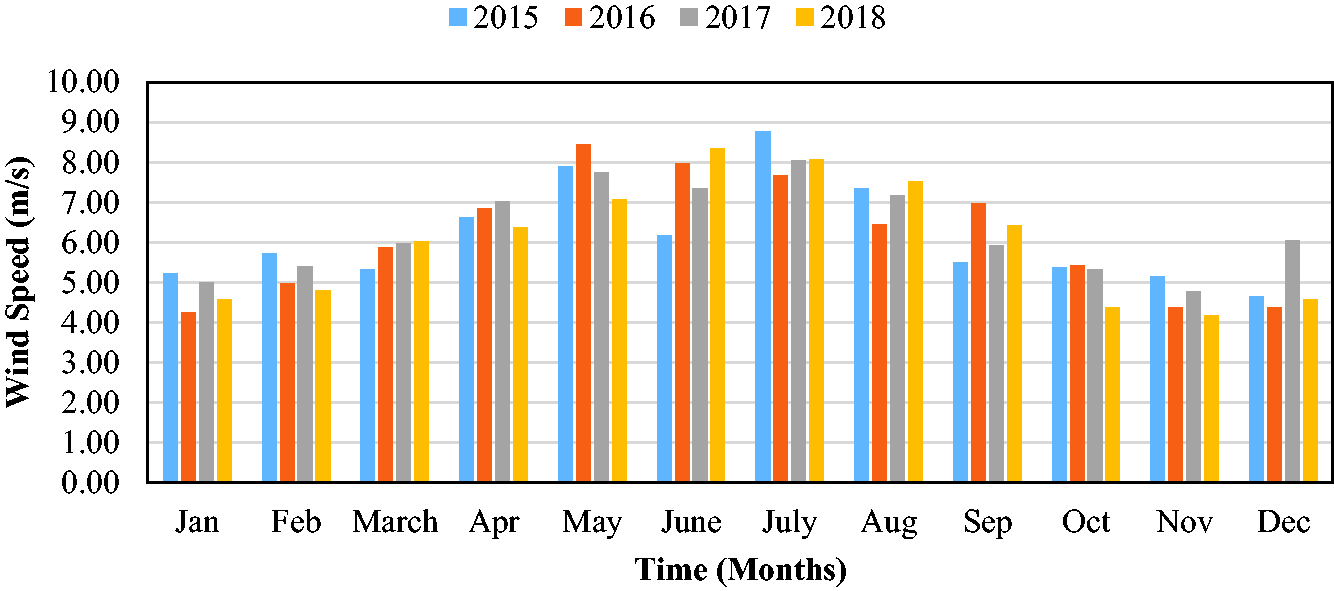
Variation observed in wind speed at Shahbandar on monthly basis.

Figure 12.

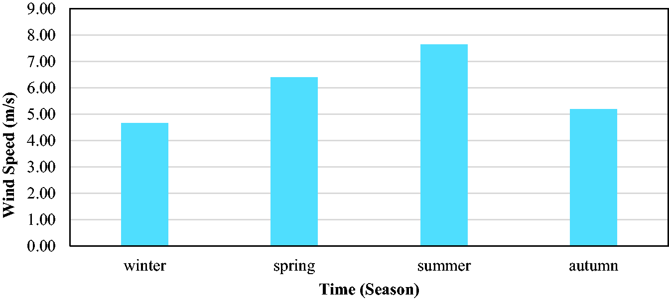
Variation observed in wind speed at Jhirk on Seasonal basis.

Figure 13.

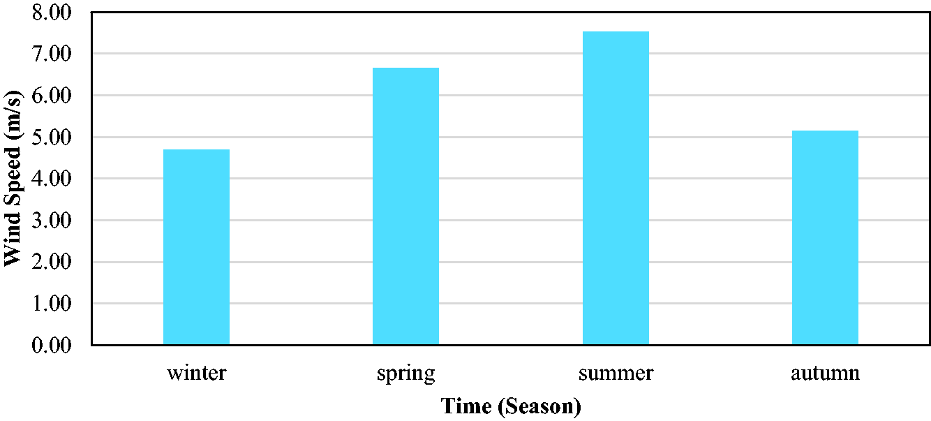
Variation observed in wind speed at Keti on Seasonal basis.

Figure 14.

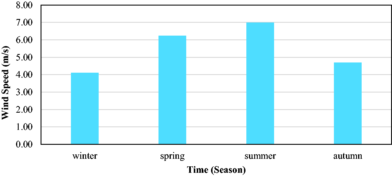
Variation observed in wind speed at Manora on Seasonal basis.

Figure 15.

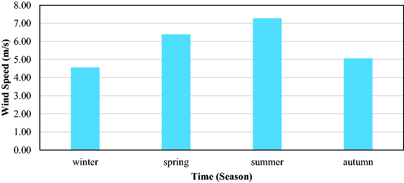
Variation observed in wind speed at Port Qasim on Seasonal basis.

Figure 16.

Variation observed in wind speed at Shahbandar on Seasonal basis.

Figure 17.

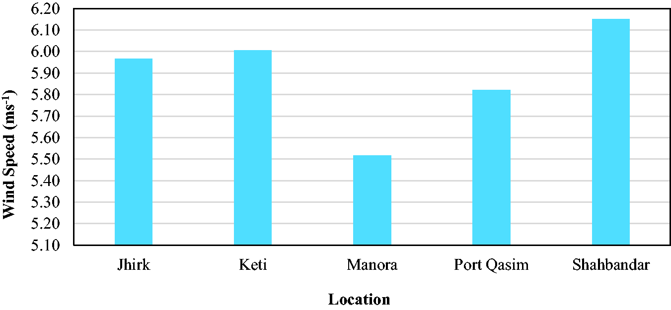
Comparison of Average wind speeds at five investigated stations.

Figure 18.

Variation observed in wind power density at Jhirk on monthly basis.

Figure 19.

Variation observed in wind power density at Keti on monthly basis.

Figure 20.

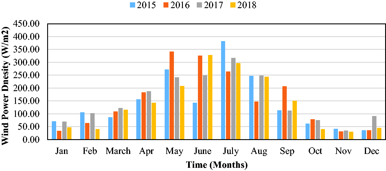
Variation observed in wind power density at Manora on monthly basis.

Figure 21.

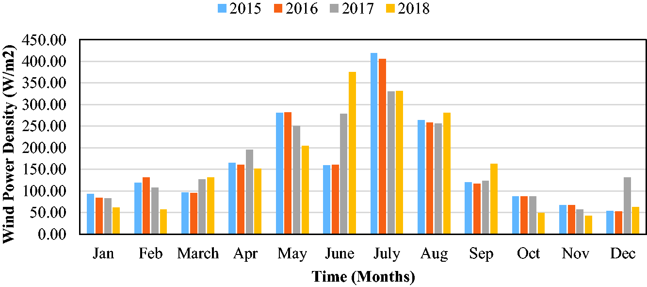
Variation observed in wind power density at Port Qasim on monthly basis.

Figure 22.

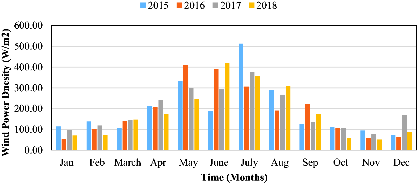
Variation observed in wind power density at Shahbandar on monthly basis.

Figure 23.

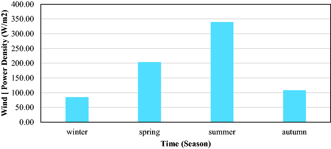
Variation observed in wind power density at Jhirk on seasonal basis.

Figure 24.

Variation observed in wind power density at Keti on seasonal basis.

Figure 25.

Variation observed in wind power density at Manora on seasonal basis.

Figure 26.

Variation observed in wind power density at Port Qasim on seasonal basis.

Figure 27.

Variation observed in wind power density at Shahbandar on seasonal basis.

Table 5.

Monthly average wind power densities (W/m²) at each station.

	Jan	Feb	March	Apr	May	June	July	Aug	Sep	Oct	Nov	Dec
Jhirk
2015	93.60	111.43	104.26	148.29	305.94	204.14	427.21	274.67	133.87	117.73	89.18	68.75
2016	60.78	80.45	140.34	195.15	473.54	387.31	328.32	146.94	245.72	96.44	58.59	71.42
2017	86.24	94.16	118.18	212.59	267.87	390.33	321.03	272.44	122.68	86.29	70.17	154.87
2018	61.63	68.26	123.50	157.76	195.42	527.00	412.76	380.88	188.10	44.79	44.11	60.02
Keti
2015	102.99	128.32	96.52	203.79	331.28	175.69	504.59	305.14	127.01	93.85	73.60	59.68
2016	44.08	91.47	126.07	206.32	393.20	380.51	309.84	193.06	220.51	104.07	46.66	48.55
2017	88.65	121.22	137.03	233.08	287.86	275.53	389.34	280.98	133.57	100.30	63.36	146.36
2018	64.44	56.28	136.98	166.06	243.68	389.81	361.97	294.24	173.42	53.34	43.01	78.29

Manora
2015	70.19	105.09	86.86	156.63	272.07	143.04	382.19	247.43	113.92	61.79	41.90	36.27
2016	33.66	64.05	108.46	183.00	341.49	325.40	264.04	147.51	207.12	78.15	31.24	35.99
2017	69.23	102.68	122.14	187.72	241.12	249.41	316.83	247.96	112.78	74.95	35.22	90.93
2018	47.38	40.33	115.49	142.37	207.50	327.84	296.53	244.28	150.54	40.71	30.39	45.18
Port Qasim
2015	92.83	118.41	96.97	164.51	280.95	159.04	419.39	264.21	120.11	87.41	67.47	53.78
2016	41.36	81.27	127.16	189.04	369.81	345.40	282.79	157.17	224.82	88.81	46.06	52.21
2017	83.27	107.79	127.07	195.29	250.44	278.43	330.33	255.52	122.79	87.11	57.07	131.10
2018	61.28	57.20	130.81	151.80	203.79	375.27	330.66	280.18	162.29	48.91	42.41	62.67
Shahbandar
2015	113.60	137.21	105.40	211.46	332.57	187.23	512.35	291.19	123.79	109.04	94.12	72.24
2016	54.08	102.06	138.41	208.77	410.01	391.55	305.06	189.76	219.92	105.48	58.62	62.18
2017	96.46	118.26	144.15	241.25	299.74	291.37	375.97	265.96	135.68	105.41	78.44	169.38
2018	70.65	71.89	147.20	173.96	243.31	420.17	356.71	307.05	174.28	56.76	50.92	86.91

Figure 28.

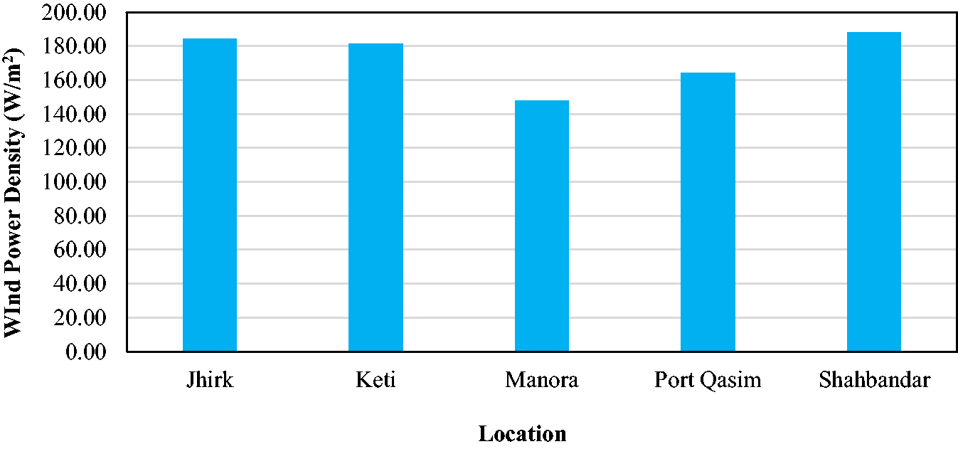
Comparison of average wind power density values at five investigated stations.

Techno economic evaluation of energy generation

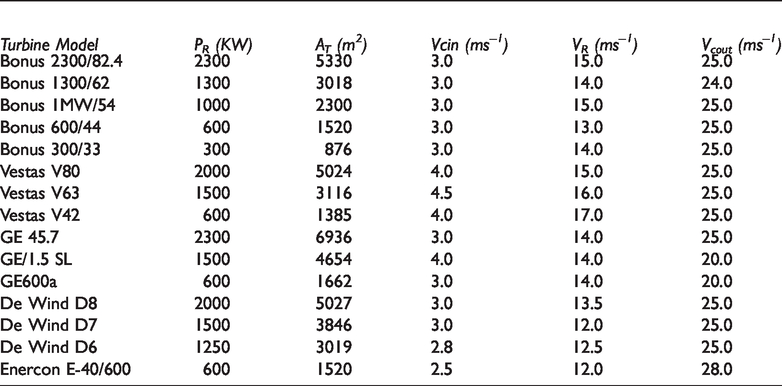
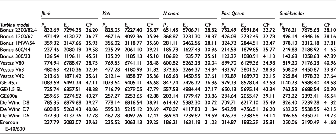
Techno-economic analysis of wind energy generation at selected locations has been made using 15 different turbines. Table 6 lists the specifications of these turbines. Based on the power produced using each turbine at each site, CFs are calculated and listed in Table 7. GE 45.7 model has been found to produce the highest amount of wind energy while Vestas V42 shows the worst performance with lowest power generation and lowest CF. Comparison among five stations shows that Shahbandar has the highest annual energy produced and Manora has the lowest for any of the turbine under consideration. This agrees with highest wind speed at Shahbandar and lowest at Manora.

Table 6.

Specifications of various turbine models.

Turbine Model	P_R (KW)	A_T (m²)	Vcin (ms^–1)	V_R (ms^–1)	V_cout (ms^–1)
Bonus 2300/82.4	2300	5330	3.0	15.0	25.0
Bonus 1300/62	1300	3018	3.0	14.0	24.0
Bonus 1MW/54	1000	2300	3.0	15.0	25.0
Bonus 600/44	600	1520	3.0	13.0	25.0
Bonus 300/33	300	876	3.0	14.0	25.0
Vestas V80	2000	5024	4.0	15.0	25.0
Vestas V63	1500	3116	4.5	16.0	25.0
Vestas V42	600	1385	4.0	17.0	25.0
GE 45.7	2300	6936	3.0	14.0	25.0
GE/1.5 SL	1500	4654	4.0	14.0	20.0
GE600a	600	1662	3.0	14.0	20.0
De Wind D8	2000	5027	3.0	13.5	25.0
De Wind D7	1500	3846	3.0	12.0	25.0
De Wind D6	1250	3019	2.8	12.5	25.0
Enercon E-40/600	600	1520	2.5	12.0	28.0

Table 7.

Power produced, P_P (kW), annual energy produced, E_P, (MWh and CF, (%) at each station using 15 turbines.

	Jhirk			Keti			Manora			Port Qasim			Shahbandar
Turbine model	P_p	E_p	CF	P_p	E_p	CF	P_p	E_p	CF	P_p	E_p	CF	P_p	E_p	CF
Bonus 2300/82.4	832.69	7294.35	36.20	825.05	7227.40	35.87	651.45	5706.71	28.32	752.49	6591.84	32.72	876.21	7675.63	38.10
Bonus 1300/62	471.49	4130.27	36.27	467.16	4092.36	35.94	368.87	3231.30	28.37	426.08	3732.49	32.78	496.14	4346.16	38.16
Bonus 1MW/54	359.32	3147.66	35.93	356.02	3118.77	35.60	281.11	2462.56	28.11	324.72	2844.51	32.47	378.10	3312.18	37.81
Bonus 600/44	237.46	2080.19	39.58	235.29	2061.10	39.21	185.78	1627.43	30.96	214.59	1879.85	35.77	249.88	2188.92	41.65
Bonus 300/33	136.54	1196.11	45.51	135.29	1185.13	45.10	106.82	935.77	35.61	123.39	1080.91	41.13	143.68	1258.63	47.89
Vestas V80	774.94	6788.47	38.75	769.53	6741.11	38.48	600.82	5263.23	30.04	699.70	6129.36	34.98	819.20	7176.23	40.96
Vestas V63	480.63	4210.36	32.04	477.28	4180.99	31.82	372.65	3264.37	24.84	433.97	3801.57	28.93	508.09	4450.87	33.87
Vestas V42	213.63	1871.42	35.61	212.14	1858.37	35.36	165.63	1450.95	27.61	192.89	1689.72	32.15	225.84	1978.32	37.64
GE 45.7	1083.59	9492.24	47.11	1073.64	9405.11	46.68	847.74	7426.22	36.86	979.23	8578.04	42.58	1140.23	9988.40	49.58
GE/1.5 SL	725.74	6357.51	48.38	716.79	6279.05	47.79	557.58	4884.44	37.17	650.13	5695.14	43.34	763.53	6688.54	50.90
GE600a	259.65	2274.52	43.27	257.27	2253.65	42.88	203.14	1779.47	33.86	234.64	2055.47	39.11	273.22	2393.41	45.54
De Wind D8	785.35	6879.68	39.27	778.14	6816.54	38.91	614.42	5382.30	30.72	709.71	6217.10	35.49	826.40	7239.28	41.32
De Wind D7	600.85	5263.43	40.06	595.33	5215.12	39.69	470.07	4117.83	31.34	542.98	4756.51	36.20	632.25	5538.55	42.15
De Wind D6	472.30	4137.36	37.78	467.78	4097.76	37.42	369.84	3239.82	29.59	426.78	3738.58	34.14	496.66	4350.71	39.73
Enercon E-40/600	237.79	2083.07	39.63	235.52	2063.13	39.25	186.21	1631.18	31.03	214.87	1882.29	35.81	250.06	2190.49	41.68

As previously explained that only the CF cannot be a decisive parameter in the selection of a turbine, but economic analysis is also an important consideration. It is quite possible that a turbine having high CF would be relatively costly compared to some other turbine. Therefore, an economic feasibility assessment is required. Table 8 enlists values of PP and unit C against each turbine at each location. It can be observed that for all investigated locations, GE/1.5 SL (not GE 45.7) is the most economical (having lowest PP and unit C) while Vestas V63 (not Vestas V42) is the least economical among all turbines. This result strengthens our argument initially made that only the CF cannot be a performance representative. Therefore, in real life, a compromise must be made in the final selection of a turbine.

Table 8.

Economic feasibility analysis of various turbine models using PP and unit cost of energy at each station.

	PP (years)					Unit cost ($/kWh)
Turbine model	Jhirk	Keti	Manora	Port Qasim	Shahbandar	Jhirk	Keti	Manora	Port Qasim	Shahbandar
Bonus 2300/82.4	7.07	7.14	9.04	7.82	6.72	0.014001	0.014130	0.017896	0.015493	0.013305
Bonus 1300/62	7.06	7.12	9.02	7.81	6.71	0.013976	0.014105	0.017864	0.015465	0.013281
Bonus 1MW/54	7.12	7.19	9.11	7.88	6.77	0.014106	0.014237	0.018031	0.015610	0.013406
Bonus 600/44	6.47	6.53	8.27	7.16	6.15	0.012807	0.012926	0.016370	0.014172	0.012171
Bonus 300/33	5.62	5.68	7.19	6.22	5.35	0.011137	0.011240	0.014235	0.012324	0.010583
Vestas V80	6.61	6.65	8.52	7.32	6.25	0.013082	0.013174	0.016873	0.014488	0.012375
Vestas V63	7.99	8.05	10.30	8.85	7.56	0.015819	0.015930	0.020403	0.017520	0.014964
Vestas V42	7.19	7.24	9.27	7.96	6.80	0.014236	0.014336	0.018361	0.015767	0.013467
GE 45.7	5.43	5.48	6.95	6.01	5.16	0.010759	0.010858	0.013752	0.011905	0.010224
GE/1.5 SL	5.29	5.36	6.89	5.91	5.03	0.010476	0.010607	0.013636	0.011695	0.009958
GE600a	5.92	5.97	7.56	6.55	5.62	0.011713	0.011821	0.014972	0.012961	0.011131
De Wind D8	6.52	6.58	8.33	7.21	6.20	0.012908	0.013028	0.016499	0.014284	0.012267
De Wind D7	6.39	6.45	8.17	7.07	6.07	0.012654	0.012771	0.016174	0.014003	0.012025
De Wind D6	6.78	6.84	8.65	7.50	6.44	0.013415	0.013545	0.017131	0.014846	0.012757
Enercon E-40/600	6.46	6.52	8.25	7.15	6.14	0.012789	0.012913	0.016333	0.014154	0.012162

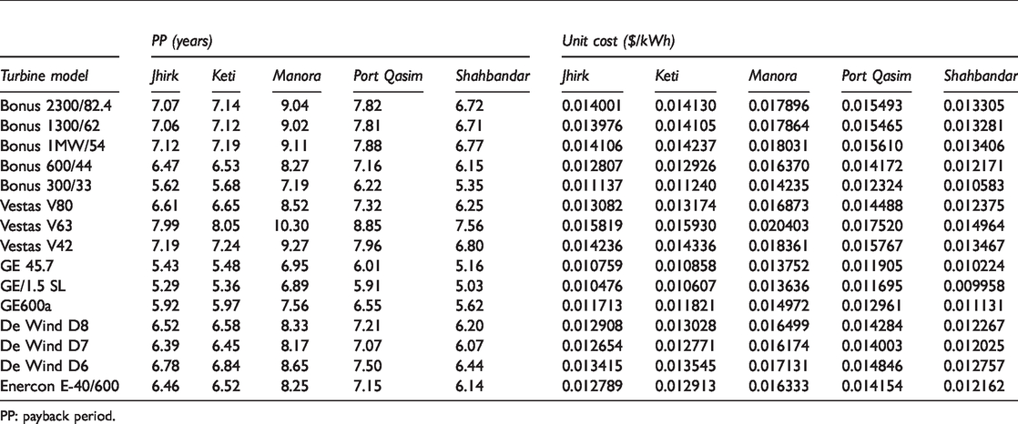
PP: payback period.

Validation of results

What is the validity of the results obtained in a study? This important question has been answered using historical data validation technique. Various probability distributions have been applied and compared and the results, thus obtained, have been validated using historical data (Khahro et al., 2014a, 2014b; Manwell et al., 2010; Morgan et al., 2011; Pobočíková et al., 2017; Rajapaksha and Perera, 2016; Sumair et al., 2020e; Silveira et al., 2019; Yilmaz and Çelik, 2011; Zhou et al., 2010).

Conclusion

Key points concluded from this work are given below:

For each of the investigated location, Normal distribution has been found the best distribution followed by Weibull, Gamma, Chi-Squared, and Rayleigh. Therefore, reliance on Weibull distribution at each location is not reasonable and advised.

Monthly and seasonal variation shows that wind resource potential is highest in July and lowest in January at all locations.

Among all locations under study, Shahbandar possesses the maximum potential whereas Manora possesses the minimum.

With respect to energy generation, GE 45.7 shows the best performance while Vestas V42 shows the least. However, economic analysis shows that GE/1.5 SL is the most economical while Vestas V63 is the least.

Therefore, turbine selection should be based on not only the energy production but also the economy depending upon which of these two factors is the main concern for wind power projects investors.

Footnotes

Declaration of conflicting interests

The author(s) declared no potential conflicts of interest with respect to the research, authorship, and/or publication of this article.

Funding

The author(s) received no financial support for the research, authorship, and/or publication of this article.

ORCID iD

Muhammad Sumair

References

Aized

Sohail Rehman

Kamran

, et al. (2019) Design and analysis of wind pump for wind conditions in Pakistan. Advances in Mechanical Engineering 11(9): 1–18.

Aman

Jasmon

Ghufran

, et al. (2013) Investigating possible wind energy potential to meet the power shortage in Karachi. Renewable and Sustainable Energy Reviews 18: 528–542.

Andrade

CFd

Maia Neto

Costa Rocha

, et al. (2014) An efficiency comparison of numerical methods for determining Weibull parameters for wind energy applications: A new approach applied to the northeast region of Brazil. Energy Conversion and Management 86: 801–808.

Arslan

Bulut

Yavuz

(2014) Comparative study of numerical methods for determining Weibull parameters for wind energy potential. Renewable and Sustainable Energy Reviews 40: 820–825.

Bagiorgas

Mihalakakou

Rehman

, et al. (2012) Wind power potential assessment for seven buoys data collection stations in Aegean Sea using Weibull distribution function. Journal of Renewable and Sustainable Energy 4(1): 013119.

Bagiorgas

Mihalakakou

Rehman

, et al. (2016) Wind power potential assessment for three buoys data collection stations in the Ionian Sea using Weibull distribution function. International Journal of Green Energy 13(7): 703–714.

Baseer

Meyer

Rehman

, et al. (2017) Wind power characteristics of seven data collection sites in Jubail, Saudi Arabia using Weibull parameters. Renewable Energy 102: 35–49.

Bassyouni

Gutub

Javaid

, et al. (2015) Assessment and analysis of wind power resource using weibull parameters. Energy Exploration & Exploitation 33(1): 105–122.

Gul

Tai

Huang

, et al. (2019) Assessment of wind power potential and economic analysis at Hyderabad in Pakistan: Powering to local communities using wind power. Sustainability 11(5): 1391.

10.

Khahro

Tabbassum

Soomro

, et al. (2014a) Evaluation of wind power production prospective and Weibull parameter estimation methods for Babaurband. Energy Conversion and Management 78: 956–967.

11.

Khahro

Tabbassum

Soomro

, et al. (2014b) Techno-economical evaluation of wind energy potential and analysis of power generation from wind at Gharo, Sindh Pakistan. Renewable and Sustainable Energy Reviews 35: 460–474.

12.

Kollu

Rayapudi

Narasimham

, et al. (2012) Mixture probability distribution functions to model wind speed distributions. International Journal of Energy and Environmental Engineering 3(1): 27.

13.

Lollchund

Boojhawon

Rughooputh

(2014) Statistical modelling of wind speed data for Mauritius. International Journal of Renewable Energy Research 4(4): 1056–1064.

14.

Manwell

McGowan

Rogers

(2010) Wind Energy Explained: Theory, Design and Application. Chichester: Wiley.

15.

Morgan

Lackner

Vogel

, et al. (2011) Probability distributions for offshore wind speeds. Energy Conversion and Management 52(1): 15–26.

16.

Pobočíková

Sedliačková

Michalková

(2017) Application of four probability distributions for wind speed modeling. Procedia Engineering 192: 713–718.

17.

Rajapaksha

Perera

(2016) Wind speed analysis and energy calculation based on mixture distributions in Narakkalliya, Sri Lanka. Journal of the National Science Foundation of Sri Lanka 44(4): 409–416.

18.

Ross

(2009) Probability and Statistics for Engineers and Scientists. New Delhi: Elsevier.

19.

Ross

(2014) Introduction to Probability and Statistics for Engineers and Scientists. MA, USA: Elsevier Science.

20.

Safari

Gasore

(2010) A statistical investigation of wind characteristics and wind energy potential based on the Weibull and Rayleigh models in Rwanda. Renewable Energy 35(12): 2874–2880.

21.

Seguro

Lambert

(2000) Modern estimation of the parameters of the Weibull wind speed distribution for wind energy analysis. Journal of Wind Engineering and Industrial Aerodynamics 85(1): 75–84.

22.

Shami

Ahmad

Zafar

, et al. (2016) Evaluating wind energy potential in Pakistan's three provinces, with proposal for integration into national power grid. Renewable and Sustainable Energy Reviews 53: 408–421.

23.

Shoaib

Siddiqui

Amir

, et al. (2017) Evaluation of wind power potential in Baburband (Pakistan) using Weibull distribution function. Renewable and Sustainable Energy Reviews 70: 1343–1351.

24.

Silveira

Gomes-Silva

Brito

, et al. (2019) Normal-G class of probability distributions: Properties and applications. Symmetry 11(11): 1407.

25.

Sumair

Aized

Gardezi

SAR

, et al. (2020a) Investigation of wind shear coefficients and their effect on annual energy yields along the coastal sites of Pakistan. Energy Exploration & Exploitation. Epub ahead of print 15-06-2020. DOI: 10.1177/0144598720930422.

26.

Sumair M, Aized T, Gardezi SAR, et al. (2020b) A novel method developed to estimate Weibull parameters. Energy Reports 6: 1715–1733.

27.

Sumair

Aized

Gardezi

SAR

, et al. (2020c) A newly proposed method for Weibull parameters estimation and assessment of wind potential in Southern Punjab. Energy Reports 6: 1250–1261.

28.

Sumair

Aized

Gardezi

SAR

, et al. (2020d) Wind potential estimation and proposed energy production in Southern Punjab using Weibull probability density function and surface measured data. Energy Exploration & Exploitation 0(0): 1–19.

29.

Sumair M, Aized T, Gardezi SAR, et al. (2020e). Comparison of three probability distributions and techno-economic analysis of wind energy production along the coastal belt of Pakistan. Energy Exploration & Exploitation. Epub ahead of print 19 June 2020. DOI: 10.1177/0144598720931587

30.

Ullah

Chaudhry

Q-U-Z

Chipperfield

(2010) An evaluation of wind energy potential at Kati Bandar. Renewable and Sustainable Energy Reviews 14(2): 856–861.

31.

Walpole

Myers

, et al. (2011) Probability & Statistics for Engineers & Scientists. Upper Saddle River, NJ: Pearson Prentice Hall.

32.

Yilmaz

Çelik

(2011) A statistical approach to estimate the wind speed distribution: The case of Gelibolu region. Doğuş Üniversitesi Dergisi 9(1): 122–132.

33.

Zhou

Erdem

, et al. (2010) Comprehensive evaluation of wind speed distribution models: A case study for North Dakota sites. Energy Conversion and Management 51(7): 1449–1458.

Application of five continuous distributions and evaluation of wind potential at five stations using normal distribution

Abstract

Keywords

Introduction

Materials and methods

Normal distribution

Gamma distribution

Chi square distribution

Weibull distribution

Rayleigh distribution

Performance comparison of distributions

Wind power density

Energy Generation Effectiveness Analysis

Results and discussions

Comparison of probability distributions

Monthly and seasonal variation in wind speed and wind power density

Techno economic evaluation of energy generation

Validation of results

Conclusion

Footnotes

Declaration of conflicting interests

Funding

ORCID iD

References