Sage Journals: Discover world-class research

Abstract

This paper deals with short-term load forecasting for energy management systems in small and middle-sized buildings. Unlike existing studies that focus on the forecasting accuracy, this study examined some candidate load forecasting methods with regard to convenience and cost-efficiency. Three-year energy use patterns of office buildings were identified according to calendar data and weather data. Simple forecasting equations were derived based on regression analyses using linear, seasonal linear, and quadratic models. The quadratic model was found most appropriate for Korea’s climate with four distinct seasons. The forecasting equation derived from the energy consumption of 2017 was verified by comparing the energy consumption forecast obtained by applying the weather data of 2018 to the equation and the actual energy consumption of 2018. This study will be using our simple load forecasting system that does not need to install sensors in all the target buildings but only in some representative buildings of similar shapes and calculate energy consumption forecasts for each target building by using the least possible data.

Keywords

Building energy energy consumption energy management system load forecasting regression analysis

Introduction

An energy management system (EMS) facilitates efficient energy use by monitoring and controlling the energy supply and demand. Generally, the EMS is utilized to operate a nationwide power grid that encompasses generation, transmission, and distribution. Traditionally, power generation was concentrated in large plants and the energy thus produced was consumed in remote cities or plants. A nationwide EMS was appropriate for this purpose. However, renewable energy systems are installed near users; therefore, EMS is required for small-scale consumers such as cities, building complexes, and plants. In power plant construction, the conventional large-scale EMS has been used to reflect the load forecasts and stably operate power transmission and distribution systems (Amjady and Daraeepour, 2010; Cerjan et al., 2019; Hyndman and Fan, 2009; Zhang et al., 2019). Recently, a small-scale EMS was used to predict the energy consumption in a building or a plant to determine the optimal size of the renewable energy source and calculate the installed capacity of the ESS. Such an EMS is also used to determine the charge and discharge capacities and cycles of the ESS, which are valuable data for reducing the energy cost (Wen et al., 2019). Accordingly, the importance of load forecasting technologies for EMS is recognized not only by operators of traditional power grids but also by energy managers of plants and buildings (Ferrari et al., 2019; Finck et al., 2019).

Load forecasting methods are mainly classified into engineering methods, statistical methods, and artificial intelligence-based methods (Fallah et al., 2019). Engineering methods predict the energy consumption based on the detailed data of the building characteristics, HVAC system, and weather conditions, which influence the energy performance. DOE-2, EnergyPlus, BLAST, ESP-r, and many other software programs have been developed for this purpose (Glavan et al., 2019; Zhang and Wen, 2019; Zhao and Magoulès, 2012). Several mechanical and architectural engineers have actively employed engineering methods. Engineering methods are accurate but demand extensive detailed information on building and environmental parameters.

Statistical methods are most widely implemented for load forecasting. These methods utilize data related to past energy consumptions, calendar data, and weather data (Fan and Hyndman, 2011). Regression analysis is mainly used to calculate a forecasting equation by deriving a correlation between factors influencing energy consumption and the actual energy consumption (Tso and Yau, 2007). Stochastic methods, exponential smoothing methods (Taylor, 2011), and ARIMA method (Huang and Shih, 2003; Taylor and McSharry, 2007) are examples of such methods. Statistical methods can hardly respond to unprecedented changes like addition of equipment and extension of building.

Artificial neural network (ANN) and support vector machine (SVM) are the most representative artificial intelligence-based methods (Barman and Choudhury, 2019; Bashir and EL-Hawary, 2009; Chen et al., 2009; Hong and Fan, 2019; Lee et al., 2019; Taylor and Buizza, 2002). Since 2000, many studies have been actively conducted for large-scale load forecasting from the perspective of a power grid operator. Unlike statistical methods, ANN-based and SVM-based methods can extract a non-linear correlation between various types of data; therefore, the accuracy of these methods is higher than that of the other methods (Ahmad et al., 2019). Among the studies on building load forecasting, Ekici and Aksoy (2009) analyzed the exterior types and characteristics of a building and used transparency (%), insulation thickness (cm), and direction as the input data to calculate the heating energy load. However, these methods require high CPU usage that can process a complex algorithm in real time (Bouktif et al., 2019; Gao et al., 2019).

Based on the above three types of load forecasting methods, many studies have proposed various modified forecasting models, analyzed their applications, and compared their performances. However, except the study by Rueda et al. (2019), all the studies focused on the accuracy of the forecasting models. In contrast, this study is mainly interested in a simple and cost-efficient load forecast that can be easily installed for the EMS in a building. Since 2017, the South Korea government has mandated the installation of EMS in the new building with an area of 10,000 m² or more. For the efficient management of energy in small buildings, simple and low-cost forecasting models for building below 10,000 m² without the need to install EMS are present in this paper. Owners of small and middle-sized buildings want to reduce energy costs by a certain degree without large investment in equipment or constant maintenance. Accordingly, this study employs statistical methods that utilize only easily accessible data, rather than artificial intelligence-based methods, which require extensive data and constant CPU operation, or engineering methods, which require the information on major energy-use equipment and building characteristics.

Regression models, semi-parametric models, exponential smoothing models, autoregressive moving average models in statistical methods are well known (Hong and Fan, 2016). Geng et al. (2018) describe linear regression models with inflection points according to outdoor temperature for use in building energy performance diagnosis. Various regression models, including multiple linear models, polynomial models, and hybrid artificial intelligence models are verified in a variety of applications: home (Fumo and Biswas, 2015; Tso and Yau, 2007), holiday (Wi et al., 2011), natural gas consumption (Soldo et al., 2014).

Semi-parametric models are based on regression models but with adding non-linear components. Fan and Hyndman (2011) proposed model adds lagged actual demand as the default input for weather effects. Goude et al. (2014) proposed an optimum semi-parametric model that uses calendar information and temperature as its primary input to 2200 substations in France and adds holiday and daylight saving time. It showed the ability to predict a huge number of energy consumptions on the distribution grid in France.

Exponential smoothing models reduce the weight of historical energy data exponentially over time. Taylor and Mcsharry (2007) have suggested exponential smoothing models with good accuracy, but they are suitable for stable weather conditions in large areas such as the national scale (Hong et al., 2014). Autoregressive moving average (ARMA) models provide two polynomials: autoregressive models and moving-average models. Although Pappas et al. (2010) and Lee and Ko (2011) use this models to produce meaningful results, there are has rich class and subjective that require a lot of data. This is sometimes an obstacle to application (Dudek, 2016).

As mention above, there are various statistical models, each with their own advantage. As is well known, energy consumption pattern varies according to various circumstances, such as season, weather, economy, area, etc. This study targets a simple and low-cost load forecasting method for office buildings in South Korea with four distinct seasons.

Background

Objective

As mentioned in Introduction, the main interest of this study is not high accuracy but the realization of a simple and cost-efficient load forecasting method that can be used in office buildings. Figure 1 shows our ultimate objective. It is assumed that the energy consumption pattern will be similar depending on the type of building, such as homes, offices, and stores. Energy usage sensor will be installed only some buildings. Where the sensor is installed, the energy consumption is predicted by the simple regression models proposed in this paper. In the absence of sensors, data from neighboring buildings with sensor and easily available information such as electric bills will be used. Our ultimate objective is to implement a load forecasting system that does not need to install sensors in all the target buildings but only in some sample buildings of similar shapes, as depicted in Figure 1, to enable the calculation of load forecasts for each target building by using the least possible data (Chen et al., 2009; Fan et al., 2019).

Figure 1.

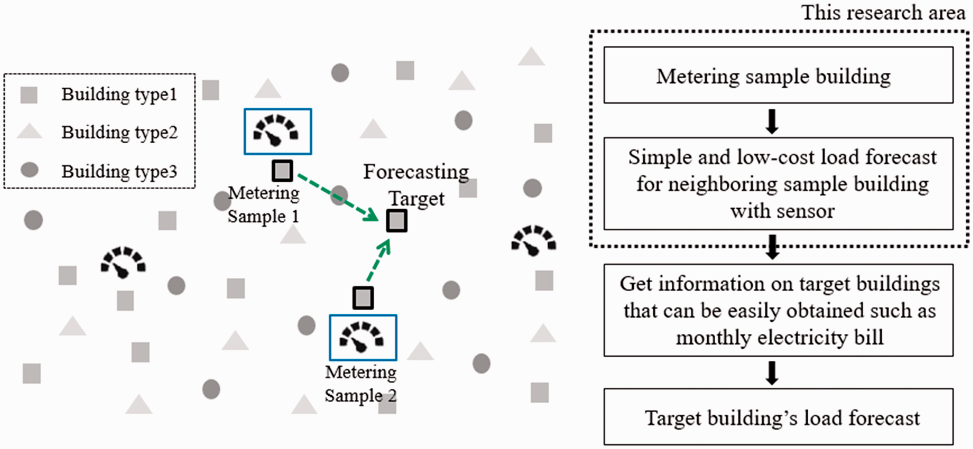
Our project’s ultimate objective and this research overview.

Weather in Korea

The Republic of Korea lies in the temperate zone and experiences four distinct seasons. Geographically, it is located in the middle latitudes of the Northern Hemisphere. Each season has different wind directions, rainfall characteristics. The winter weather is cold and dry owing to the influence of the Siberian high-pressure system, whereas the summer weather is hot and humid because of the North Pacific anticyclone. The rainy season or monsoon starts from the middle of June in the southern region and continues for approximately 30 days. Accordingly, the summer rainfall accounts for as much as 50–60% of the annual total rainfall. In most parts of the nation, the annual average humidity ranges from 60% to 75%. In July and August, the average humidity reaches up to 70–85%. Spring and autumn are influenced by migratory anticyclones and are associated with clear and dry days. The average humidity of March and April, which are the months of spring, is 50–70%. Figure 2 shows the daily average temperature, humidity, wind speed and solar radiation of a particular region in Korea from 2016 to 2018. The temperatures are high during summer, that is, from June to August, and fall below zero in winter, that is, from November to February Thus, the temperature variation indicates the four distinct seasons of Korea (Min et al., 2011).

Figure 2.

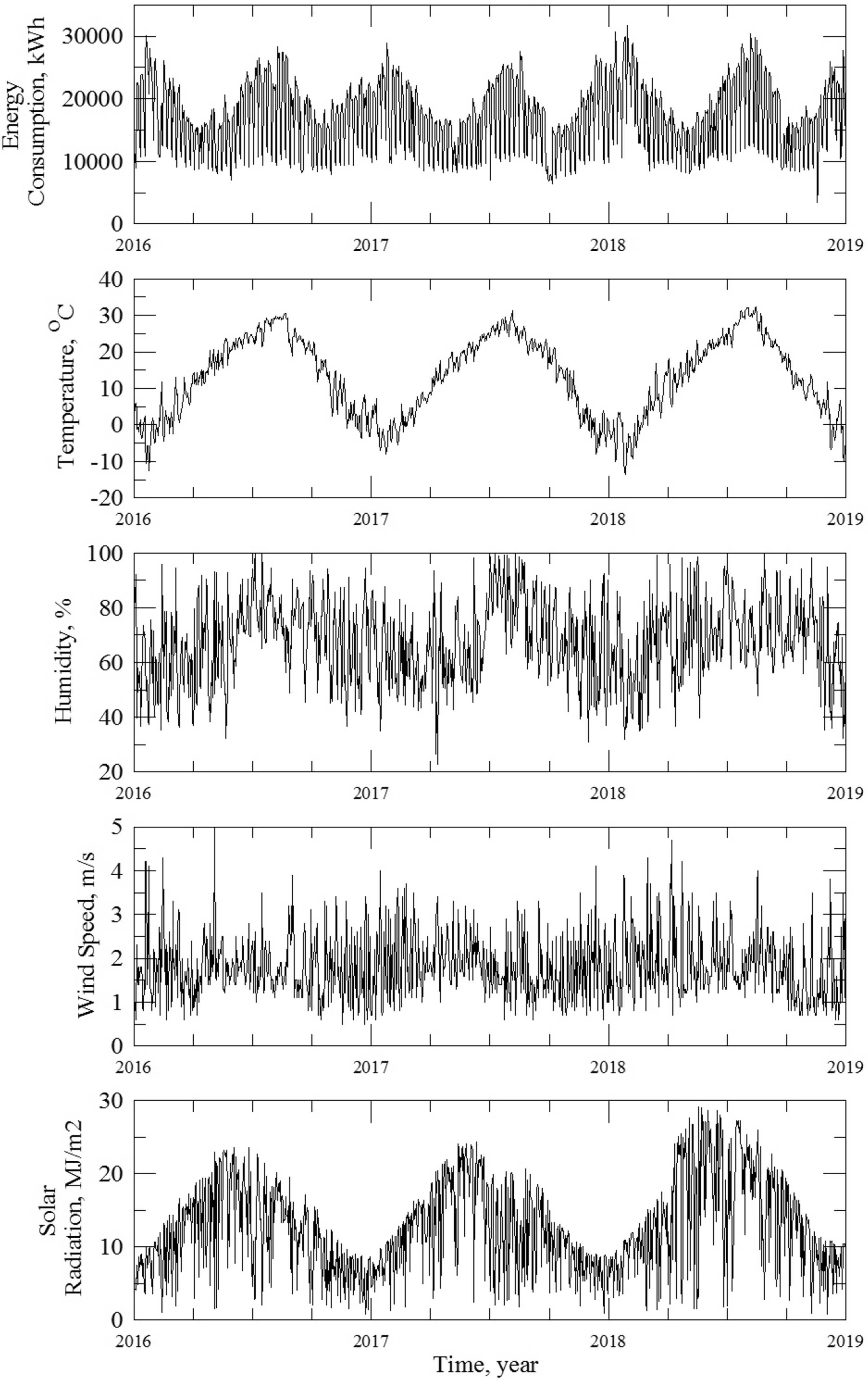
Trends of energy consumption in sample buildings from 2016 to 2018 and trends of daily average temperature, humidity, wind speed and solar radiation for the same period in Korea. The same pattern with the highest temperature in summer and the lowest temperature in winter is repeated in the one-year intervals.

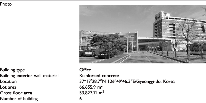
Sample building

A group of six buildings with gross area of 53,828 m² was selected as the sample. Totally, 111 knowledge enterprises have offices in these buildings. As of 2017, the total energy consumption was 5,789 MWh, which was mostly supplied by the power grid. This study used load data collected at 15 min intervals by the telemetering system of Korea Electric Power Corporation (KEPCO), which operates the power grid of Korea. This study also utilized the hourly and daily weather data, which were provided by the Korea Meteorological Administration (KMA). The weather data, namely, temperature, wind speed, solar radiation, and humidity, were measured at an observatory located 16 km from the sample buildings. The humidity measurements were obtained eight times (03:00, 06:00, 09:00, 12:00, 15:00, 18:00, 21:00, 24:00) a day (Table 1).

Table 1.

Sample buildings information.

Photo
Building type	Office
Building exterior wall material	Reinforced concrete
Location	37°17′28.7″N 126°49′46.3″E/Gyeonggi-do, Korea
Lot area	66,655.9 $m^{2}$
Gross floor area	53,827.71 $m^{2}$
Number of building	6

Table 2.

Simple linear model of weather and energy consumption from 2016 to 2018.

Year	Day	Temperature		Wind speed		Humidity		Solar radiation
Year	Day	Formula	MAPE	Formula	MAPE	Formula	MAPE	Formula	MAPE
2018	Weekday	−23.2x + 20,586	22.76	838.4x + 18,737	22.81	−59.5x + 24,339	22.49	−49.2x + 20,969	22.60
2018	Weekend	−93.3x + 12,381	18.80	860.4x + 9660.2	18.47	−62.1x + 15,296	18.37	−40.8x + 11,779	18.96
2017	Weekday	−75.5x + 20,072	21.52	−264.6x + 19,647	22.19	28.7x + 17,265	21.95	−81.3x + 20,163	21.88
2017	Weekend	−57.8x + 10,929	12.64	302.3x + 9685.9	12.69	−1.8x + 10,341	12.65	−70.5x + 11,063	12.08
2016	Weekday	−12.6x + 19,765	19.86	351.6x + 18,964	19.89	−0.785x + 19,648	19.90	−36.8x + 20,026	9.04
2016	Weekend	−90.5x + 11,912	13.10	543.0x + 9707.9	13.78	−22.6x + 12,220	13.61	−69.6x + 11,432	12.90

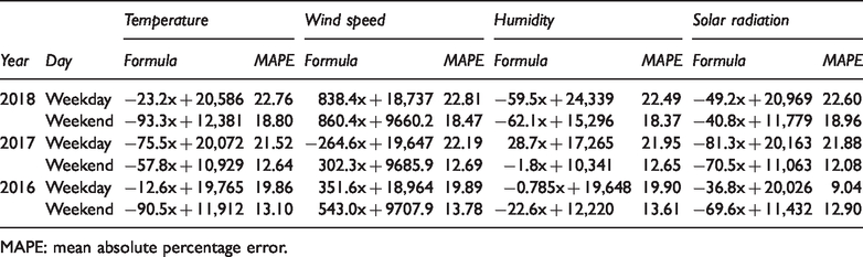
MAPE: mean absolute percentage error.

Simple load forecasting method

Correlation between weather and building energy consumption

Figure 3 illustrates a correlation between energy consumption of the sample building and temperature, wind speed, humidity, and solar radiation. As mentioned previously, the goal of this study was not to achieve high accuracy but to identify a simple and cost-efficient load forecasting method. In this regard, wind speed, humidity, and solar radiation show little correlation with energy consumption. On the other hand, temperature displays a clear hockey stick-shaped correlation with the energy consumption (Moral-Carcedo and Pérez-García, 2019; Xie et al., 2016). In Figure 3(a), the energy consumption according to temperature is distributed into the upper and lower parts, which correspond to weekdays and weekends, respectively. Beyond the temperature of approximately 13°C, the energy consumption increased with rising temperature. At temperatures below this, the energy consumption increased as the temperature decreased. It can be inferred that the air-conditioning system was operated at high temperatures, whereas the heating system was operated at low temperatures, both of which increased the energy consumption.

Figure 3.

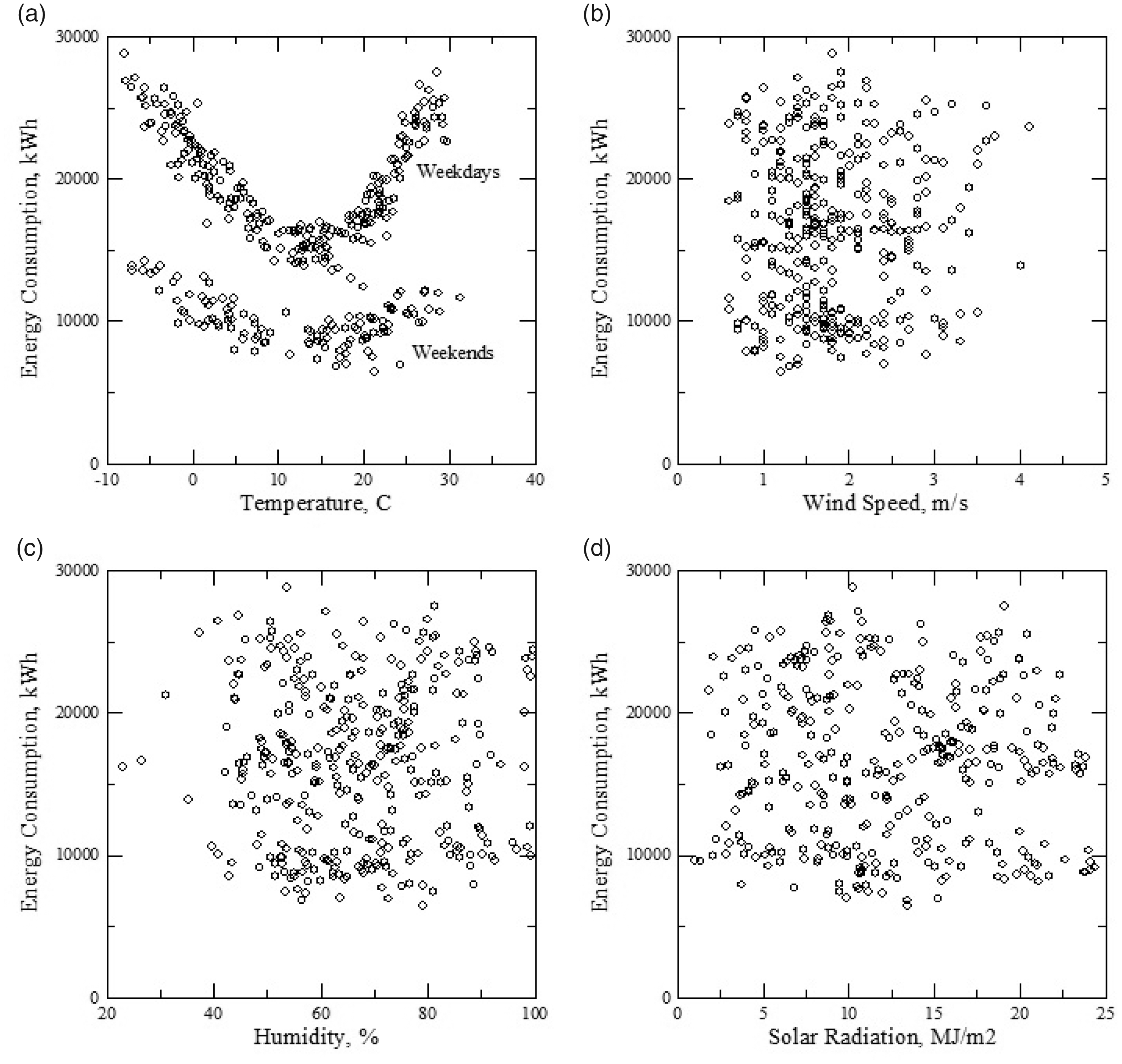
Correlation between the energy consumption of a sample building and (a) temperature, (b) wind speed, (c) humidity, and (d) solar radiation in the year 2017. Temperature and energy consumption show a hockey stick-shaped correlation.

Regression model

As illustrated in Figure 4, there are three types of regression analysis models. Figure 4(a) is a simple linear model suitable for regions with temperate climate. This model was utilized by Fumo and Biswas (2015).

f (x) = α_{1} x + β_{1}

(1)

Figure 4.

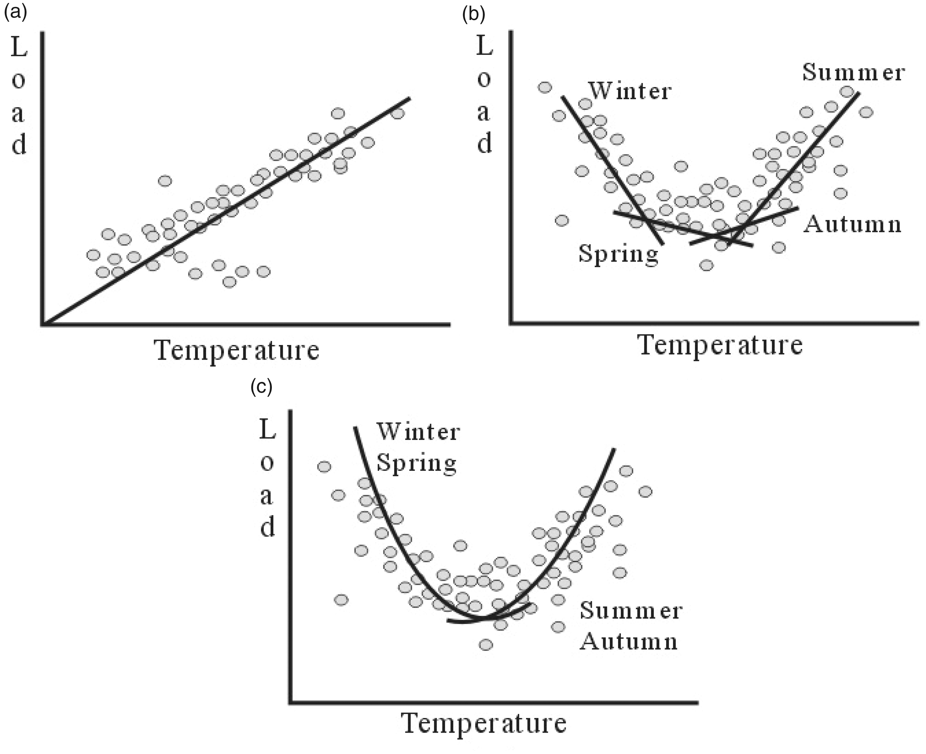
(a) Simple linear, (b) seasonal linear and (c) quadratic models.

α₁ is the sensitivity of the energy consumption to temperature and β₁ denotes the base load. This does not seem to be suitable for Korea, which has four distinct seasons including winter.

Geng et al. (2018) distinguished between the heating degree-day (HDD) section with a linear decrease and cooling degree-day (CDD) section with a linear increase by using a correlation between building energy consumption and temperatures of a particular region in China. The results of applying this distinction to the four distinct seasons of Korea are illustrated in Figure 4(b).

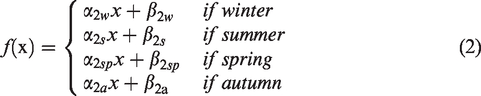
The HDD section corresponds to winter, the CDD section corresponds to summer, and the no degree-day (NDD) section, which is less sensitive to temperatures, is allocated to spring and autumn, as expressed in the following equation.

f (x) = {\begin{array}{l} α_{2 w} x + β_{2 w} i f winter \\ α_{2 s} x + β_{2 s} i f summer \\ α_{2 s p} x + β_{2 s p} i f spring \\ α_{2 a} x + β_{2 a} i f autumn \end{array}

(2)

Valor et al. (2001) conducted a regression analysis of the energy consumption and temperatures in Spain by using quadratic equations (Wi et al., 2011).

f (x) = {\begin{array}{l} α_{3 w} x^{2} + β_{3 w} x + γ_{w} i f winter, spring \\ α_{3 s} x^{2} + β_{3 s} x + γ_{s} i f summer, autumn \end{array}

(3)

The first coefficient (α₃) indicates the efficiency of the cooling and heating systems at high or low temperatures. The second coefficient (β₃) denotes the inflection temperatures of cooling and heating, and the third constant (γ) is the base load that is constant irrespective of temperature.

As the increase in energy consumption exceeds the increment or decrement in temperature, the energy consumptions of the cooling and heating systems can be described more faithfully.

The regression analysis applied the daily average temperature, wind speed, humidity, and solar radiation as the independent variables and the daily energy consumption as a dependent variable. The accuracy of the regression analysis model was expressed by mean absolute percentage error (MAPE), which is the difference in absolute values between the actual and estimated data.

MAPE = \frac{1}{N} \sum_{i = 1}^{N} \frac{| A_{i} - P_{i} |}{A_{i}} \times 100

(4)

N denotes the number of datasets, A_i is the actual load and P_i indicates the load forecast.

Short-term load forecasting in sample buildings

Single regression analysis

Tables 2 to 4 present the regression analysis results by applying the simple linear model, the seasonal linear model, and the quadratic model discussed in Section 3 to the daily energy consumption of the sample buildings mentioned in Section 2. Weekdays and weekends were distinguished in the analysis.

The MAPE in the case of the regression analysis using the simple linear model was mostly over 20%. In other words, the linear model could not express the energy consumption accurately. As mentioned previously, this model was not appropriate for regions that experience both winter and summer.

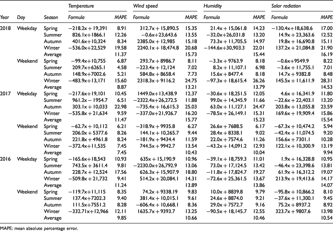
The seasonal linear model may produce different results depending on how the inflection points of CDD, NDD, and HDD are designated. As this study focused on economy and user convenience, four seasons were adopted as followed by KEPCO, which is the charging authority for energy consumption in Korea. In other words, CDD and HDD were allocated to summer (June to August) and winter (November to February), respectively. NDD was allocated to both spring (March to May) and autumn (September and October). The regression analysis results obtained under this assumption are provided in Table 3. |α| in equation (2) indicates the sensitivity of energy consumption to temperature and is higher on weekdays than on weekends. This result is expected because the sample building contains offices. Moreover, spring showed a negative energy sensitivity (α) like winter, and autumn showed a positive energy sensitivity (α) like summer.

Table 3.

Seasonal linear model of weather and energy consumption from 2016 to 2018.

Year	Day	Season	Temperature		Wind speed		Humidity		Solar radiation
Year	Day	Season	Formula	MAPE	Formula	MAPE	Formula	MAPE	Formula	MAPE
2018	Weekday	Spring	−218.2x + 19,391	8.91	312.7x + 15,890.5	15.35	21.4x + 15,061.8	14.23	−130.4x+18,638.6	17.00
		Summer	826.1x+1866.1	12.26	−0.6x+23,643.6	13.55	−32.0x+26,031.8	13.20	14.9x + 23,363.6	12.52
		Autumn	401.6x+10,324	8.34	2385.0x + 12,985	15.18	73.3x + 11,705.5	14.97	19.8x + 16,690.8	15.11
		Winter	−536.0x+22,529	19.58	2240.1x + 18,474.8	20.68	−144.6x+30,903.3	22.01	137.2x + 21,084.8	21.90
		Average		11.37		15.73		15.44		16.19
	Weekend	Spring	−99.4x+10,755	6.87	293.7x + 8986.7	8.11	−3.3x + 9763.9	8.18	−0.6x+9549.9	8.22
		Summer	209.7x+6265.1	4.58	−223.4x + 12,124	7.02	8.2x + 11,107.1	6.98	−3.6x + 11,755.1	7.01
		Autumn	148.9x+7002.6	5.21	584.8x + 8658.4	7.73	15.6x + 8477.4	8.18	14.7x + 9382.8	8.48
		Winter	−483.9x+13,171	15.60	2318.3x + 9116.2	24.75	−97.3x + 18,615.4	26.26	145.5x + 11,611.9	28.31
		Average		8.87		13.21		13.79		14.53
2017	Weekday	Spring	−217.6x+19,101	10.45	1449.0x+13,438.9	12.37	−30.6x + 18,251.5	12.05	4.6x + 16,341.9	11.80
		Summer	961.2x − 1954.7	6.51	−2322.4x+26,272.5	11.88	99.0x + 14,345.9	11.66	−22.6x + 22,403.1	13.20
		Autumn	303.1x + 10,033	22.98	−735.4x + 16,615.3	25.03	63.0x + 11,127.1	24.47	203.8x + 13,055.8	23.59
		Winter	−535.8x + 21,634	9.59	−337.0x+21,926.7	16.20	−78.5x + 26,149.1	15.31	169.6x + 19,909.4	15.86
		Average		11.47		15.77		15.23		15.54
	Weekend	Spring	−62.7x + 10,112	6.21	−318.9x + 9935.8	6.27	26.6x + 7688.5	6.17	−67.3x + 10,474.2	5.94
		Summer	206.0x + 5377.6	8.26	144.1x + 10,265.7	9.44	28.4x + 8338.1	9.02	−42.4x + 11,074.5	9.20
		Autumn	221.8x + 4961.8	8.24	−181.9x + 9434.4	11.59	22.0x + 7574.6	11.26	156.6x + 7301.1	10.28
		Winter	−372.4x+11,535	7.45	744.5x + 9942.7	13.54	−43.2x + 14,091.2	12.93	122.1x + 10,300.9	13.19
		Average		7.45		10.43		10.04		9.94
2016	Weekday	Spring	−165.6x+18,543	10.93	635x + 15,190.9	10.96	−39.1x + 18,759.3	11.01	1.9x + 16,328.8	10.95
		Summer	743.5x + 3611.4	9.81	−2230.0x+26,792.9	13.06	73.0x + 17,124.5	13.42	−46.4x + 23,398.6	13.81
		Autumn	228.7x + 12,524	17.56	626.3x + 15,907.9	18.80	−11.8x + 17,824.7	19.27	61.9x + 16,312.2	19.07
		Winter	−509.8x + 21,732	9.41	514.2x + 20,084.1	14.31	−72.6x + 25,361.5	13.67	213.9x + 19,413.6	14.17
		Average		11.24		13.89		13.86		14.07
	Weekend	Spring	−119.7x+11,115	8.35	74.2x + 9338.19	9.83	10.0x + 8839.8	9.79	−95.8x + 10,866.2	8.10
		Summer	137.4x+7202.3	9.40	381.4x + 10,015.1	9.61	24.6x + 8874.0	9.21	−37.6x + 11,300.1	9.45
		Autumn	111.5x+7551.2	8.28	−606.4x + 10,668.1	8.36	29.0x + 7572.7	9.16	75.2x + 8937.2	8.92
		Winter	−332.71x+12,966	12.11	1635.7x + 9393.7	13.25	−90.5x + 18,145.7	12.55	323.7x + 9807.6	13.98
		Average		9.85		10.66		10.46		10.54

MAPE: mean absolute percentage error.

Table 4 presents the results of the quadratic regression analysis. As was expected, temperature had a higher correlation with energy consumption than wind speed, humidity, and solar radiation. In most cases, the sensitivity to temperature (α) and the base load (γ) were higher on weekdays than on weekends. In addition, as α is higher in summer than in winter, the cooling system caused a larger increase in energy consumption according to temperature than the heating system.

Table 4.

Quadratic model of weather and energy consumption from 2016 to 2018.

Year	Day	Season	Temperature		Wind speed		Humidity		Solar radiation
Year	Day	Season	Formula	MAPE	Formula	MAPE	Formula	MAPE	Formula	MAPE
2018	Weekday	Spring/Winter	11.8x2 − 568.4x+21,856.9	10.28	−324.2x2 + 2014.7x+17,411.4	21.18	2.6x2 − 464.8x+38,125.9	18.62	−16.3x2 + 171.1x+20,740.2	17.58
	Weekday	Summer/Autumn	25.3x2 − 410.3x+16,427.5	12.13	−1091.4x2 + 6597.1x+12,992.7	23.52	−0.35x2 + 95.7x+15,941.5	24.02	9.3x2 − 103.4x+19,715.4	23.74
	Average			11.06		22.16		20.88		20.15
	Weekend	Spring/Winter	17.2x2 − 504.7x+12,649.2	11.16	−82.6x2 + 1417.3x+9285.1	24.57	2.1x2 − 358.7x+24,865.0	22.12	−12.0x2 + 245.1x+10,680.5	24.03
	Weekend	Summer/Autumn	4.3x2 + 34.1x+7786.6	5.03	−956.1x2 + 4233x+6705.4	9.71	0.8x2 − 119.2x+15,193.9	11.17	3.0x2 − 34.4x+10,320.1	10.36
	Average			8.57		18.28		17.49		18.24
2017	Weekday	Spring/Winter	18.1x2 − 653.2x+21,163.6	9.51	1756.8x2 − 7777x+26,695.5	18.14	0.5x2 − 102.0x+23,581.6	19.50	−27.9x2 + 442.1x+18,604.3	17.56
	Weekday	Summer/Autumn	45.3x2 − 1079.8x+19,972.6	13.86	−1370x2 + 4783x+15,461	25.87	−0.5x2 + 232.0x+4759.7	23.23	31.0x2 − 590.1x+20,402.5	24.22
	Average			11.21		21.16		20.96		20.16
	Weekend	Spring/Winter	11.9x2 − 343.1x+11,375.0	7.18	533.3x2 − 1865.6x+11,752.5	12.60	2.5x2 − 348.1x+21,746.6	12.40	−8.7x2 + 111.0x+10,632.5	11.89
	Weekend	Summer/Autumn	1.9x2 + 138.0x+5844.6	8.19	−479.2x2 + 2053.8x+7990	12.12	0.2x2 − 0.7x+8635.8	11.44	4.3x2 − 116.5x+10,539.0	12.23
	Average			7.58		12.41		12.02		12.02
2016	Weekday	Spring/Winter	19.9x2 − 662.4x+21,223.9	9.20	−30.7x2 + 668.3x+17,898.5	18.03	−0.8x2 + 37.5x+19,827.7	17.36	−21.2x2 + 272.0x+19,182.7	16.03
	Weekday	Summer/Autumn	31.9x2 − 717.9x+19,238.1	13.19	−2177.9x2 + 8762.7x+12,515.8	20.64	−5.2x2 + 832.4x−12,314.0	20.74	0.8x2 + 208.3x+17,560	20.81
	Average			10.87		19.12		18.77		18.03
	Weekend	Spring/Winter	14.1x2 − 454.2x+12,645.0	8.99	76.7x2 + 451.5x+9873.9	15.81	1.8x2 − 271.7x+20,795.7	15.45	−19.7x2 + 335.1x+10,217.7	13.70
	Weekend	Summer/Autumn	0.9 + 100.2x+7525.0	8.98	−112.5x2 + 335.2x+10,088	10.54	−1.1x2 + 190.3x+2461.2	10.06	−6.1x2 + 195.4x+9011.2	9.92
	Average			8.99		13.60		13.19		12.12

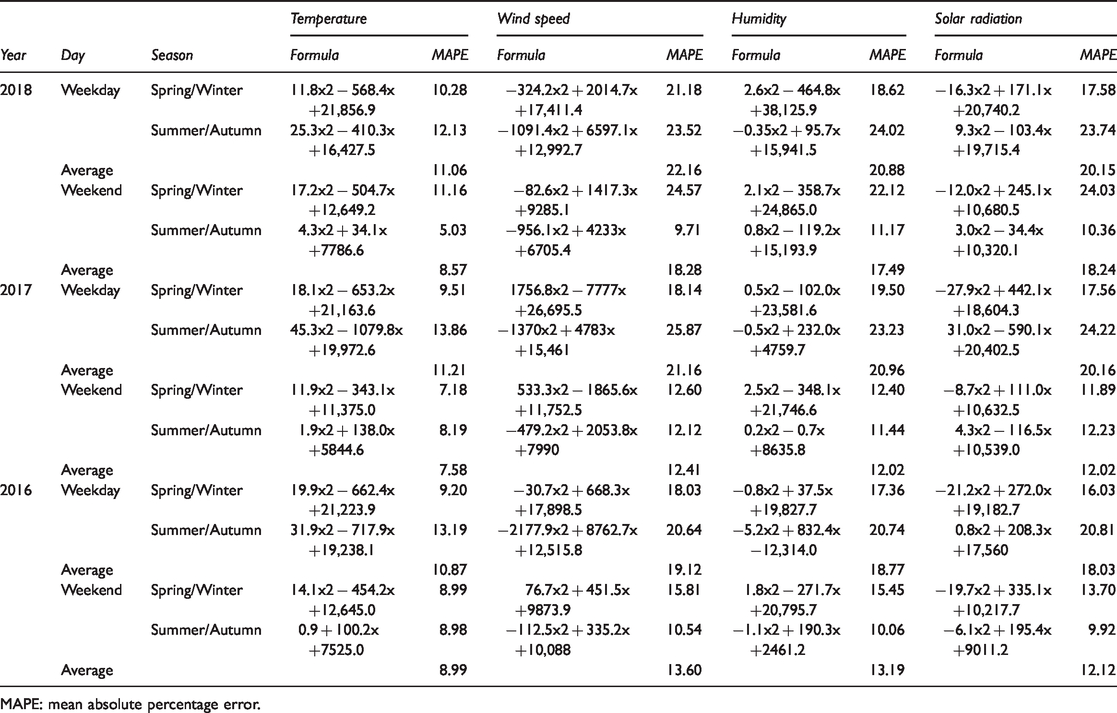
MAPE: mean absolute percentage error.

Among the three models, the quadratic model had the lowest MAPE. Although, the MAPE of the quadratic model was only approximately 0.2% lower than that of the seasonal linear model, the former was lower both on weekdays and on weekends from 2016 to 2018. Consequently, the quadratic model was selected as most appropriate for the weather in Korea.

Multiple regression analysis

The results of the multiple regression analysis using the quadratic model expressed in equation (5) are presented in Table 5. In equation (5), t is temperature and k denotes wind speed, humidity, or solar radiation. As shown in Figure 2, wind speed, humidity, and solar radiation also have sinusoidal shapes such as temperature; therefore, they also used the quadratic function.

f (x) = {\begin{array}{l} α_{4 w} t^{2} + β_{4 w} t + α_{5 w} k^{2} + β_{5 w} k + γ_{2 w} i f winter, spring \\ α_{4 s} t^{2} + β_{4 s} t + α_{5 s} k^{2} + β_{5 s} k + γ_{2 s} i f summer, autumn \end{array}

(5)

Table 5.

Multiple regression analysis for temperature, additional weather factor, and energy consumption.

Year	Day	Season	Wind speed		Humidity		Solar radiation
Year	Day	Season	Formula	MAPE	Formula	MAPE	Formula	MAPE
2018	Weekday	Spring/Winter	11.3t²−567.1t−334.5k²+1378.3k + 20,776.5	10.26	12.8t²−610.4t + 0.12k²+15.7k + 20,467.9	10.06	13.8t²−568.8t + 6.2k²−279.2k + 23,782.9	9.53
	Weekday	Summer/Autumn	26t²−448.7t + 203.7k²−431.8k + 16,916.4	12.07	31.9t²−677.8t−0.52k²+177.4k + 8603.5	10.97	27.5t²−461.1t + 2.1k²−166k + 18,448.2	11.79
	Average			11.02		10.44		10.47
	Weekend	Spring/Winter	16.1t²−487.9t−35.2k²+597.7k + 11,743.3	11.09	18.4t²−530.5t + 0.07k²+5.9k + 12,010	11.02	16.5t²−508.3t + 3.9k²−102.6k + 13,265.5	10.95
	Weekend	Summer/Autumn	4.4t²+25.4t + 28.2k²+33.7k + 7741.6	4.95	4.9t²+6.6t + 0.6k²−79.1k + 10,574.4	4.96	4.3t²+42.4t−0.1k²−18.6k + 7939.8	5.02
	Average			8.49		8.46		8.44
2017	Weekday	Spring/Winter	18t²−648.7t + 166.6k²−1091.6k + 22,544	9.54	18.9t²−669.1t + 0.68k²−67.5k + 22,640	9.49	17.4t²−667t + 10.4k²−241.3k + 22,396.4	9.26
	Weekday	Summer/Autumn	44.2t²−1030.4t + 46.5k²−551.3k + 20,238.1	13.84	45.1t²−1129.2t + 0.87k²−72k + 21,524	13.57	48.1t²−1216.2t + 15.9k²−391.8k + 23,405.4	13.64
	Average			11.22		11.09		10.97
	Weekend	Spring/Winter	12.8t²−358.4t−117.7k²+358.2k + 11,192.9	7.08	13.4t²−368.3t−0.28k²+47.7k + 9520.7	7.07	11.5t²−344.8t + 0.0004k²+12.5k + 11,270	7.15
	Weekend	Summer/Autumn	1.04t²+180t + 109.7k²−181.8k + 5327.5	8.12	2.3t²+124.5t + 0.60k²−88.7k + 9128.2	8.15	2.3t²+123.7t + 0.58k²−9.7k + 6005.5	8.22
	Average			7.49		7.50		7.57
2016	Weekday	Spring/Winter	19.7t²−658.8t + 45.9k²−53.3k + 21,133.4	9.12	20.1t²−668.7t + 0.28k²−31k + 22,035.5	9.16	20.8t²−671.3t + 8.1k²−249.2k + 22,649.3	8.68
	Weekday	Summer/Autumn	33.1t²−780.2t−266.4k²+1401.8k + 18,456.3	13.26	34.6t²−822.4t + 2.04k²−268.5k + 28,548.6	13.10	30.8t²−635.1t + 11.7k²−338.4k + 20,053.3	13.13
	Average			10.85		10.81		10.54
	Weekend	Spring/Winter	10.9t²−418.2t−207.1k²+1592.3k + 10,810.5	8.18	13.2t²−445t + 1.4k²−174k + 17,944.4	8.63	17.5t²−455.9t−8.9k²+125.1k + 12,203.8	8.43
	Weekend	Summer/Autumn	2.3t²+72.6t + 651k²−2468.5k + 9463.2	8.92	2.7t²+14.2t + 0.16k²−6.4k + 8026.8	8.97	0.998t²+105.2t−2.6k²+39.5k + 7339.5	8.78
	Average			8.49		8.77		8.58

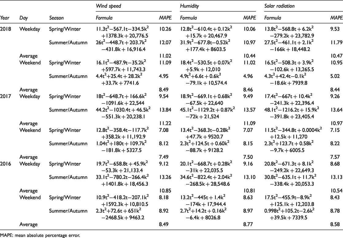
MAPE: mean absolute percentage error.

Figure 5 shows the total MAPE for each year of seasonal linear, quadratic, and multiple regression models on weekdays and weekends each year in Tables 3 to 5. The multiple regression models use humidity, which has the lowest MAPE, as a second variable (k). The difference of MAPEs is small. In most case, however, the quadratic model is better than the seasonal linear model. As the number of variables increases, the correlation coefficient becomes higher due to the structure of the regression analysis. Accordingly, the multiple regression analysis showed best MAPE values.

Figure 5.

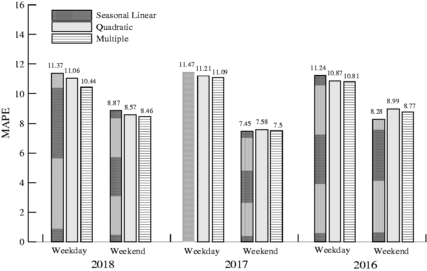
Total MAPE of seasonal linear models, quadratic models, multiple regression models on weekdays and weekends in 2016, 2017, 2018.

Hourly load forecasting

Figure 6 schematically illustrates the correlations between energy consumption and temperature, wind speed, humidity, and solar radiation at specific hours of the day (03:00, 09:00, 13:00, and 17:00) in 2017. As solar radiation exists only during the day, there is no graph for early morning and night. Although the correlation between energy consumption and temperature at early morning shows no difference between weekdays and weekends, the graphs are not significantly different from that of the daily average energy consumption in Figure 3. The forecasting equation for hourly energy consumption was calculated by regression analysis using not the daily average energy consumption but the energy consumption at each given time and the weather information. The result was similar to the daily average.

Figure 6.

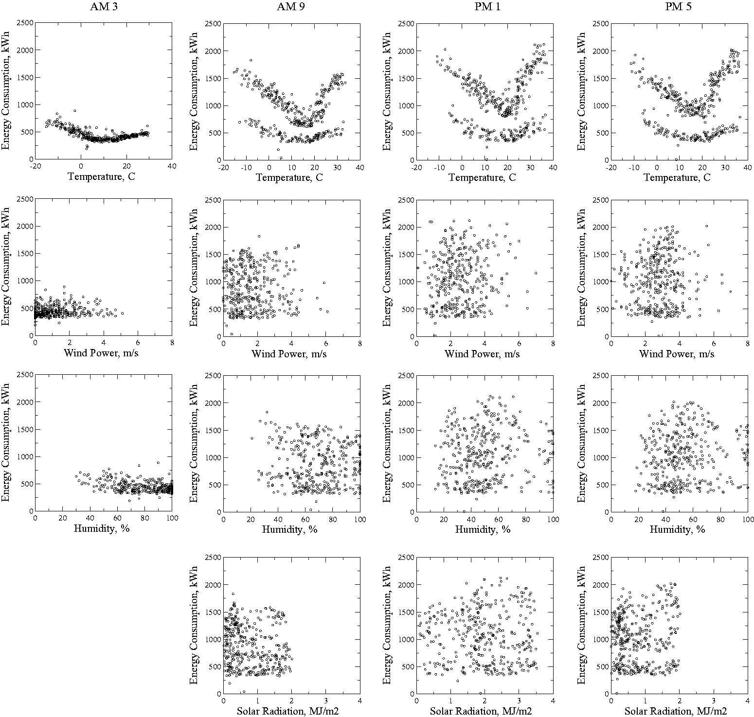
Correlation between energy consumption and weather at specific hours of the day for the year 2017. The correlation analysis between energy consumption and temperature shows a certain pattern. The correlation analyses for the remaining weather factors do not reveal such a pattern.

Verification of forecasting model

Each forecasting equation was derived based on the energy consumption and weather data of 2017. The equations thus obtained were applied to the case of 2018 and the results were compared with the actual data. Figure 7 shows the actual data and forecasting date. The values forecasted with the seasonal linear equation were −217.6x + 19,101 for weekday of spring, 916.2x − 1954.7 for weekday of summer, 303.1x + 10,033 for weekday of autumn, −535.8x + 21,634 for weekday of winter, −62.7x + 10,112 for weekend of spring, 206.0x + 5377.6 for weekend of summer, 221.8x + 4961.8 for weekend of autumn, and −372.4x + 11,535 for weekend of winter. The values forecasted with the quadratic equation were 18.1x² − 653.2x + 21,163.6 for weekday of winter/spring, 45.3x² − 1079.8x + 19,972.6 for weekday of summer/autumn, 11.9x² − 343.1x + 11,375.0 for weekend of winter/spring, and 1.931.1x² + 138.0x + 5844.6 for weekend of summer/autumn. The values forecasted with the multiple regression equation using temperature and humidity as independent variables were 18.873t²−669.064t + 0.684k²−67.516k + 22,639.998 for weekday of winter/spring, 45.144t²−1129.212t + 0.873k²−71.952k + 21,523.981 for weekday of summer/autumn, 13.437t²−368.329t−0.275k²+47.702k + 9520.7401 for weekend of winter/spring, and 2.263t²+124.522t + 0.5985k²−88.7k + 9128.1879 for weekend of summer/autumn. Here, t is temperature and k denotes humidity. Figure 7 compares the energy consumption forecasts against the actual values in 2018. The MAPEs of the seasonal linear model for weekday and weekend were 11.47 and 7.45, respectively, whereas those of the quadratic model were 11.21 and 7.58, respectively and those of the multiple regression analysis were 11.09 and 7.5, respectively.

Figure 7.

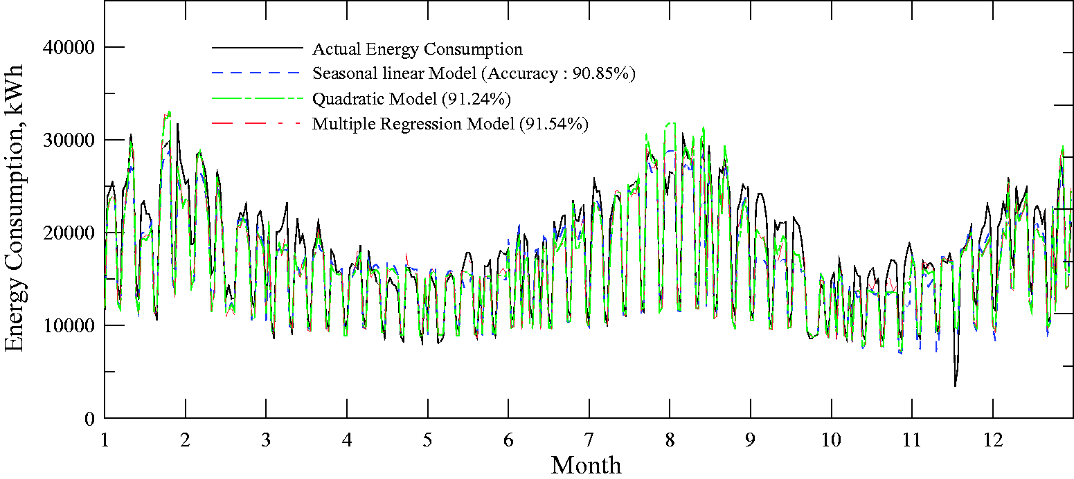
Actual energy consumption of 2018; energy consumption forecasts of the seasonal linear model, quadratic model, and multiple regression model.

Figure 8 shows the application results of the hourly forecasts for specific dates in 2018, which were designated as business days representing the four seasons. Thus, 3 April 2018 represented spring; 14 August 2018 represented summer; 2 October 2018 represented autumn; 2 January 2018 represented winter. Energy consumption forecasts were calculated by applying the data on each date to the forecasting equations. The graphs in Figure 8 show the actual energy consumptions and forecasts obtained by seasonal linear model, quadratic model and multiple regression analysis. The forecasting accuracies of the seasonal linear model were 89.33% for spring, 82.33% for summer, 93.67% for autumn, and 93.62% for winter, whereas those of the quadratic model were 89.85%, 89.08%, 92.69%, and 93.06%, respectively and those of the multiple regression analysis were 90.25%, 88.55%, 90.74%, and 93.09%, respectively.

Figure 8.

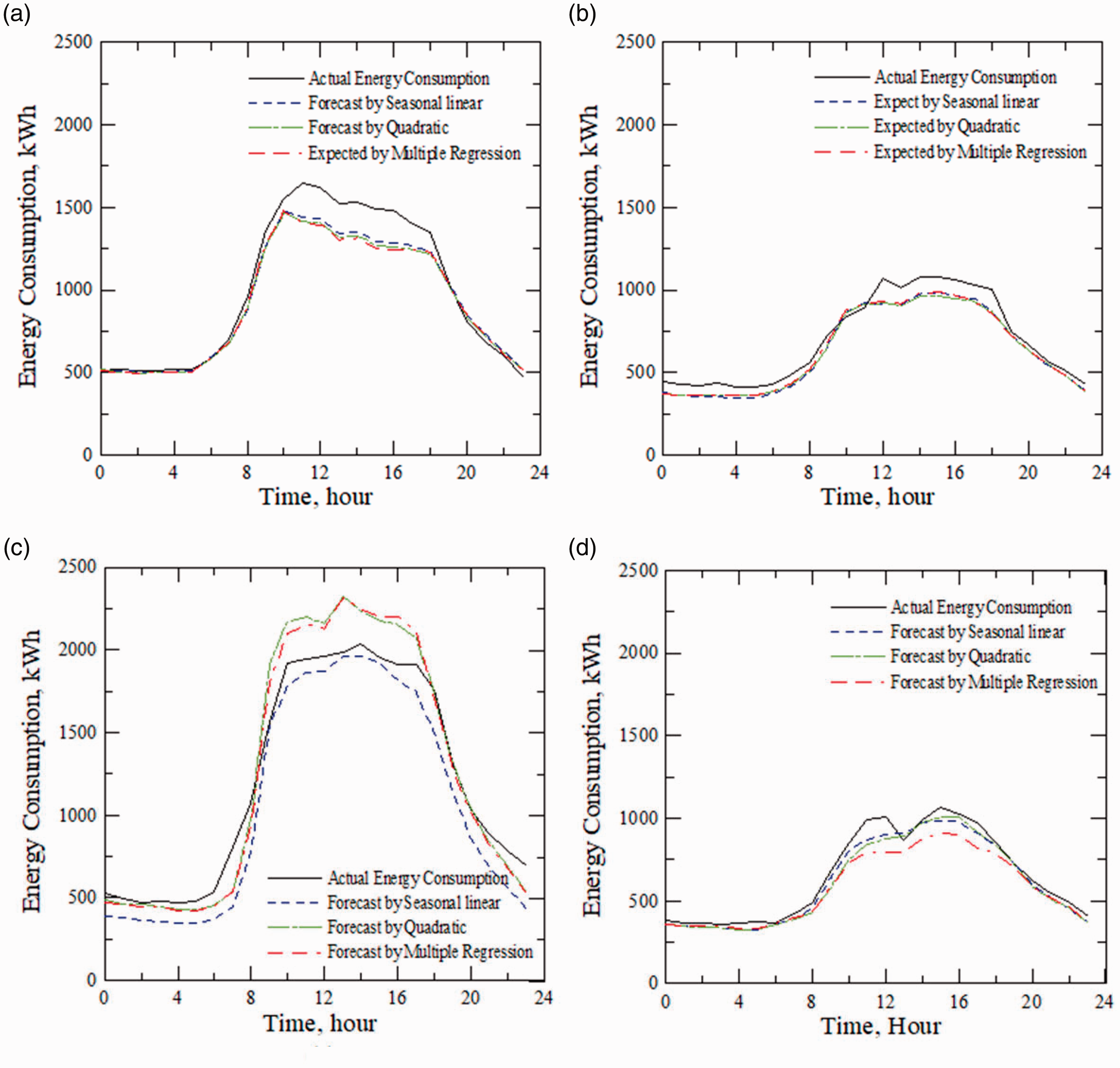
Comparison between actual values and forecasts obtained by forecasting equations for specific dates: (a) winter (2 January 2018), (b) spring (3 April 2018), (c) summer (14 August 2018), (d) autumn (2 October 2018).

Conclusion

This study examined load forecasting functions and their performance from the perspective of simplicity and cost efficiency for application to the EMSs of small and middle-sized buildings. The functions demand only limited amount of data and small investment on equipment. A statistical method was employed to produce load forecasts by using only weather data and past energy consumptions. The energy consumption of an actual building was compared with the weather data to identify a correlation. The correlations between energy consumption data and weather data such as temperature, wind speed, humidity, and solar radiation were examined by using linear, seasonal linear, and quadratic models, and through multiple regression analysis. Only temperature showed a significant correlation with the energy consumption. The quadratic model was the most appropriate for the weather of Korea, which has four distinct seasons. Accordingly, quadratic equations were derived for each season, that is, according to the temperature. When temperature increased in summer, the cooling system was operated more frequently, resulting in increased energy consumption. When temperature decreased in winter, the heating system was operated more frequently, again resulting in increased energy consumption. Forecasting equations derived from past data were applied to the weather data of 2018 to predict the energy consumption.

Comparisons of the forecasts obtained by the seasonal linear model and the seasonal quadratic simple regression analysis with the actual daily energy consumption of 2018 showed forecast accuracies of 90.85% and 91.24%, respectively. The forecast of the multiple regression analysis using temperature and humidity was 91.54% accurate. Forecasts for the hourly energy consumptions on specific dates with the seasonal linear model, the quadratic model, and the multiple regression analysis had the accuracies of 82.33%–93.67%, 89.08%–93.06%, and 88.55%–93.09%, respectively. This study did not aim for high forecasting accuracy but examined the load forecasting methods to assess their simplicity and cost efficiency. Further study will seek to improve the forecasting accuracy of such simple and cost-efficient methods by combining the measurements of a sample building and the approximate energy consumption of a target building.

Footnotes

Acknowledgements

The author would like to thank Miss Hye-jin Lee of Yeungnam University College for collecting the weather data for this paper.

Declaration of conflicting interests

The author(s) declared no potential conflicts of interest with respect to the research, authorship, and/or publication of this article.

Funding

The author(s) disclosed receipt of the following financial support for the research, authorship, and/or publication of this article: This work was supported by the Yeungnam University College Research grants in 2018.

ORCID iD

Dongho Lee

References

Ahmad

Javaid

Mateen

, et al. (2019) Short-term load forecasting in smart grids: An intelligent modular approach. Energies 12(1): 164.

Amjady

Daraeepour

(2010) Midterm demand prediction of electrical power systems using a new hybrid forecast technique. IEEE Transactions on Power Systems 26(2): 755–765.

Barman

Choudhury

NBD

(2019) Season specific approach for short-term load forecasting based on hybrid FA-SVM and similarity concept. Energy 174: 886–896.

Bashir

EL-Hawary

(2009) Applying wavelets to short-term load forecasting using PSO-based neural networks. IEEE Transactions on Power Systems 24(1): 20–27.

Bouktif

Fiaz

Ouni

, et al. (2019) Single and multi-sequence deep learning models for short and medium term electric load forecasting. Energies 12(1): 149.

Cerjan

Petričić

, and Delimar

(2019) HIRA model for short-term electricity price forecasting. Energies 12(3): 568.

Chen

Luh

Guan

, et al. (2009) Short-term load forecasting: Similar day-based wavelet neural networks. IEEE Transactions on Power Systems 25(1): 322–330.

Dudek

(2016) Pattern-based local linear regression models for short-term load forecasting. Electric Power Systems Research 130: 139–147.

Ekici

Aksoy

(2009) Prediction of building energy consumption by using artificial neural networks. Advances in Engineering Software 40(5): 356–362.

10.

Fallah

Ganjkhani

Shamshirband

, et al. (2019) Computational intelligence on short-term load forecasting: A methodological overview. Energies 12(3): 393.

11.

Fan

Guo

Zheng

, et al. (2019) Application of the weighted K-nearest neighbor algorithm for short-term load forecasting. Energies 12(5): 916.

12.

Fan

Hyndman

(2011) Short-term load forecasting based on a semi-parametric additive model. IEEE Transactions on Power Systems 27(1): 134–141.

13.

Ferrari

Zagarella

Caputo

, et al. (2019) Results of a literature review on methods for estimating buildings energy demand at district level. Energy 175: 1130–1137.

14.

Finck

Zeiler

(2019) Economic model predictive control for demand flexibility of a residential building. Energy 176: 365–379.

15.

Fumo

Biswas

(2015) Regression analysis for prediction of residential energy consumption. Renewable and Sustainable Energy Reviews 47(3): 332–343.

16.

Gao

Zhao

, et al. (2019) Short-term electricity load forecasting model based on EMD-GRU with feature selection. Energies 12(6): 1140.

17.

Geng

Lin

, et al. (2018) Building energy performance diagnosis using energy bills and weather data. Energy and Buildings 172: 181–191.

18.

Glavan

Gradišar

Moscariello

, et al. (2019) Demand-side improvement of short-term load forecasting using a proactive load management – A supermarket use case. Energy and Buildings 186: 186–194.

19.

Goude

Nedellec

Kong

(2014) Local short and middle term electricity load forecasting with semi-parametric additive models. IEEE Transactions on Smart Grid 5(1): 440–446.

20.

Hong

Fan

(2016) Probabilistic electric load forecasting: A tutorial review. International Journal of Forecasting 32(3): 914–938.

21.

Hong

Pinson

Fan

(2014) Global energy forecasting competition 2012. International Journal of Forecasting 30(2): 357–363.

22.

Hong

Fan

(2019) Hybrid empirical mode decomposition with support vector regression model for short term load forecasting. Energies 12(6): 1093.

23.

Huang

Shih

(2003) Short-term load forecasting via ARMA model identification including non-Gaussian process considerations. IEEE Transactions on Power Systems 18(2): 673–679.

24.

Hyndman

Fan

(2009) Density forecasting for long-term peak electricity demand. IEEE Transactions on Power Systems 25(2): 1142–1153.

25.

Lee

(2011) Short-term load forecasting using lifting scheme and ARIMA models. Expert Systems with Applications 38(5): 5902–5911.

26.

Lee

Jung

Lee

(2019) Prediction model based on an artificial neural network for user-based building energy consumption in South Korea. Energies 12(4): 608.

27.

Min

Kryjov

, et al. (2011) Evaluation of the weather generator CLIGEN with daily precipitation characteristics in Korea. Asia-Pacific Journal of Atmospheric Sciences 47(3): 255–263.

28.

Moral-Carcedo

Pérez-García

(2019) Time of day effects of temperature and daylight on short term electricity load. Energy 174: 169–183.

29.

Pappas

Ekonomou

Karampelas

, et al. (2010) Electricity demand load forecasting of the Hellenic power system using an ARMA model. Electric Power Systems Research 80(3): 256–264.

30.

Rueda

Cuéllar

Molina-Solana

, et al. (2019) Generalised regression hypothesis induction for energy consumption forecasting. Energies 12(6): 1069.

31.

Soldo

Potočnik

Šimunović

, et al. (2014) Improving the residential natural gas consumption forecasting models by using solar radiation. Energy and Buildings 69: 498–506.

32.

Taylor

(2011) Short-term load forecasting with exponentially weighted methods. IEEE Transactions on Power Systems 27(1): 458–464.

33.

Taylor

Buizza

(2002) Neural network load forecasting with weather ensemble predictions. IEEE Transactions on Power Systems 17(3): 626–632.

34.

Taylor

McSharry

(2007) Short-term load forecasting methods: An evaluation based on European data. IEEE Transactions on Power Systems 22(4): 2213–2219.

35.

Tso

Yau

(2007) Predicting electricity energy consumption: A comparison of regression analysis, decision tree and neural networks. Energy 32(9): 1761–1768.

36.

Valor

Meneu

Caselles

(2001) Daily air temperature and electricity load in Spain. Journal of Applied Meteorology 40(8): 1413–1421.

37.

Wen

Zhou

Yang

, et al. (2019) Optimal load dispatch of community microgrid with deep learning based solar power and load forecasting. Energy 171: 1053–1065.

38.

Joo

Song

(2011) Holiday load forecasting using fuzzy polynomial regression with weather feature selection and adjustment. IEEE Transactions on Power Systems 27(2): 596–603.

39.

Xie

Chen

Hong

, et al. (2016) Relative humidity for load forecasting models. IEEE Transactions on Smart Grid 9(1): 191–198.

40.

Zhang

Chai

(2019) Prediction of China’s energy consumption based on robust principal component analysis and PSO-LSSVM optimized by the Tabu search algorithm. Energies 12(1): 196.

41.

Zhang

Wen

(2019) A systematic feature selection procedure for short-term data-driven building energy forecasting model development. Energy and Buildings 183: 428–442.

42.

Zhao

Magoulès

(2012) A review on the prediction of building energy consumption. Renewable and Sustainable Energy Reviews 16(6): 3586–3592.

Low-cost and simple short-term load forecasting for energy management systems in small and middle-sized office buildings

Abstract

Keywords

Introduction

Background

Objective

Weather in Korea

Sample building

Simple load forecasting method

Correlation between weather and building energy consumption

Regression model

Short-term load forecasting in sample buildings

Single regression analysis

Multiple regression analysis

Hourly load forecasting

Verification of forecasting model

Conclusion

Footnotes

Acknowledgements

Declaration of conflicting interests

Funding

ORCID iD

References