Sage Journals: Discover world-class research

Abstract

The utilization of aquifer energy is a new technology closely related to the development of injection and production well technologies. Accurately predicting the effective use of geothermal energy storage in a surrounding aquifer is of great significance. A developed theory of groundwater hydro-geothermal transfer is suggested by analyzing the general features of stored energy in aquifers together with the interactions between flow connections and thermal breakthroughs. Based on the water-heat transfer in an aquifer, a coupled numerical model of groundwater flow and heat transfer is established using FEFLOW software for an injection and production wells system in the city of Xianyang to simulate the flow and temperature field. The results show that the key for the formation of a flow connection is the hydraulic gradient. That is, whether the flow connection will occur can be judged quantitatively according to the hydraulic gradient. Flow connections occur more easily through greater flow quantities and quicker injection and pumping rates, which lead to earlier occurrences of thermal breakthroughs. At an operation time of 120 days, to prevent thermal breakthroughs in the production wells, the reasonable well spacing was between 180 and 200 m, and the optimal well spacing was 180 m. This method is of great significance for the calculation of reasonable distance between injection and production wells of geothermal tail water without thermal breakthroughs and the sustainable development of a groundwater environment.

Keywords

Injection and production wells system flow connection thermal breakthrough reinjection temperature field numerical analysis

Introduction

At present, the exploitation of geothermal energy increases rapidly in cities with rich thermal reservoirs and surrounding areas; the groundwater funnel formed by underground thermal reservoir layers expands continuously; and the geothermal water resources show an obvious attenuation trend in lots of modern cities (Nam and Ooka, 2010). In this case, the implementation of an artificial recharge of geothermal water is a key measure to achieve the sustainable development and utilization of geothermal resources. Therefore, recharge is a very important component of the geothermal development process. Reinjection started as a kind of wastewater treatment method, but has now transformed into an important tool for achieving sustainable development and utilization of geothermal resources (Stefansson, 1997). However, in many new fields, the common practice is usually to convert abandoned or shallow observation wells to reinjection wells (Fukuda et al., 2005; Kaya et al., 2011; Scheiber et al., 2018). This method leads to the decrease of the effective utilization of wells; on the one hand, because of the limited capacity and the formation plug, the amount of reinjection will decrease as time goes on (Jin et al., 2014).

In many places, thermal breakthroughs are a common problem. Once thermal breakthrough occurs, it is necessary to select the location of the reinjection wells again (Ganguly, 2017; Vallejos et al., 2005; Wang et al., 2017). The process of relocation sometimes leads to the interruption of the operations process in the field (Kaya et al., 2011). If there is a connected secondary porosity (cracks) between the injection and the production wells, this phenomenon may occur very quickly. The injected water flows from the injection zone to the extraction zone and absorbs the heat energy from the rock matrix. The cold front of water flows can be detected by chemical characteristics, that is, the arrival of the thermal front of water flows (Goyal, 1999).

There are complex characteristics in the groundwater flow and temperature fields between geothermal injection and production wells. If the injected water rapidly connects from the injection well to the production well, it will lead to the occurrence of thermal breakthrough. A thermal breakthrough between injection wells and production wells can result in a decrease in boiling rate (Goyal, 1999) and a consequent decrease in heat production efficiency. Thermal breakthrough can also lead to many operational problems, including the need to adjust the structure of the well and the modification of the field operation mode (Hawkins et al., 2017; Shook, 1999). Different reinjection strategies will cause a different response of hydraulic and temperature fields within a certain area that can be affected by hydraulic and temperature fields. In order to provide early warning, a perfect early-warning monitoring scheme needs to be well established. Through monitoring the hydraulic field and temperature field variations, timely early warning can help develop an appropriate operation management strategy for injection and production wells.

In the process of geothermal development and utilization, the selection of the optimum well distance is one of the key issues. Only if the distance between the injection and production wells is chosen properly, can the best effects of development and utilization be achieved. The distance between the injection and production wells should not be too far or too close. If the distance is too far, the effects of reinjection cannot be achieved; if the distance is too close, thermal breakthrough is likely to occur and cannot achieve the purpose of geothermal energy development and utilization. That is to say, the distance between the injection and production wells should be within the influence of the hydraulic field and outside the influence scope of the thermal field. To clearly understand the layered energy distributions of the flow and temperature fields, reasonable locations of production wells must be determined to improve the utilization efficiency of underground heat storage. To prevent the occurrence of thermal breakthroughs in two-phase production zones (Willems et al., 2017), it is necessary to study the variations in the flow and temperature fields of aquifers with different compositions, and to predict changes in the distributions of state variables in the underground cold and hot water reservoirs (In the process of recharge, with the increase of the amount of recharged water, the cold water or hot water that is poured into the reservoir moves around constantly, forming “underground cold reservoir” or “underground hot water reservoir.”).

There are a lot of studies in reinjection and geothermal development fields; for example, the degree of hydraulic connectivity between injection and production wells was measured by pressure communication within the reinjection system (Evans et al., 2014; Mink et al., 2015). However, this method requires drilling first before we can obtain the available information of pressure communication. Therefore, it may not be the most effective, simple, or practically useful approach.

To protect environmental and groundwater resources, to improve the efficiency of the injection and production wells system (IPWS) and of the heat exchange, and to avoid the occurrence of secondary geological disasters (e.g., initiation of earthquakes due to thermal cracking of the rock, and collapse caused by underground water funnels) (Ganguly, 2017; Huo et al., 2011, 2016a, 2016b), studies on various characteristics of the hydraulic and temperature field of the IPWS are very necessary during long-term operating conditions.

A new method for determining the optimum distance between geothermal injection and production wells is proposed in this paper. This method can not only ensure the hydraulic connection between geothermal injection and production wells, but also improve the efficiency of reinjection, and prevent occurrence of thermal breakthrough during the operating period. This paper presents research on an IPWS project in a residential area of Xianyang, Shaanxi Province, China, based on models of the interactions between the flow connection and heat transfixion. A couple of numerical models of groundwater flow and heat transference are established based on the principle of water-heat transfer in the aquifer and the theory of pressure transient analysis (PTA) (Wang et al., 2015). In addition, a numerical analysis of the flow and temperature fields for an IPWS in Xianyang is performed to provide a reasonable determination method of the well spacing and a scientific basis for an optimal layout scheme of the injection and production wells.

Study setting

The study area

The city of Xianyang, which is located in the central part of Shaanxi Province, China, is approximately 30 km (19 miles) northwest of Xi’an, and the Weihe River flows to the south of the city (Li et al., 2013; Xi et al., 2014). The northern part of Xianyang is situated on the Chinese Loess Plateau, while the south is a part of the Weihe Plain. In general, the terrain gradually falls away from the north to the south. The city has a warm temperate continental monsoon climate and features a chilly winter and torrid summer. Overcast and rainy days are the most frequent during the summer and autumn, although extreme heat events may sear the city during the summer with temperatures in excess of 40°C (104°F). Because of the cold weather in winter, the operation of IPWS is mainly in winter for the purposes of heating and bathing. In Xianyang, an underground IPWS has been analyzed and used to simulate the groundwater flow for the study area by utilizing the FEFLOW software (Figure 1).

Figure 1.

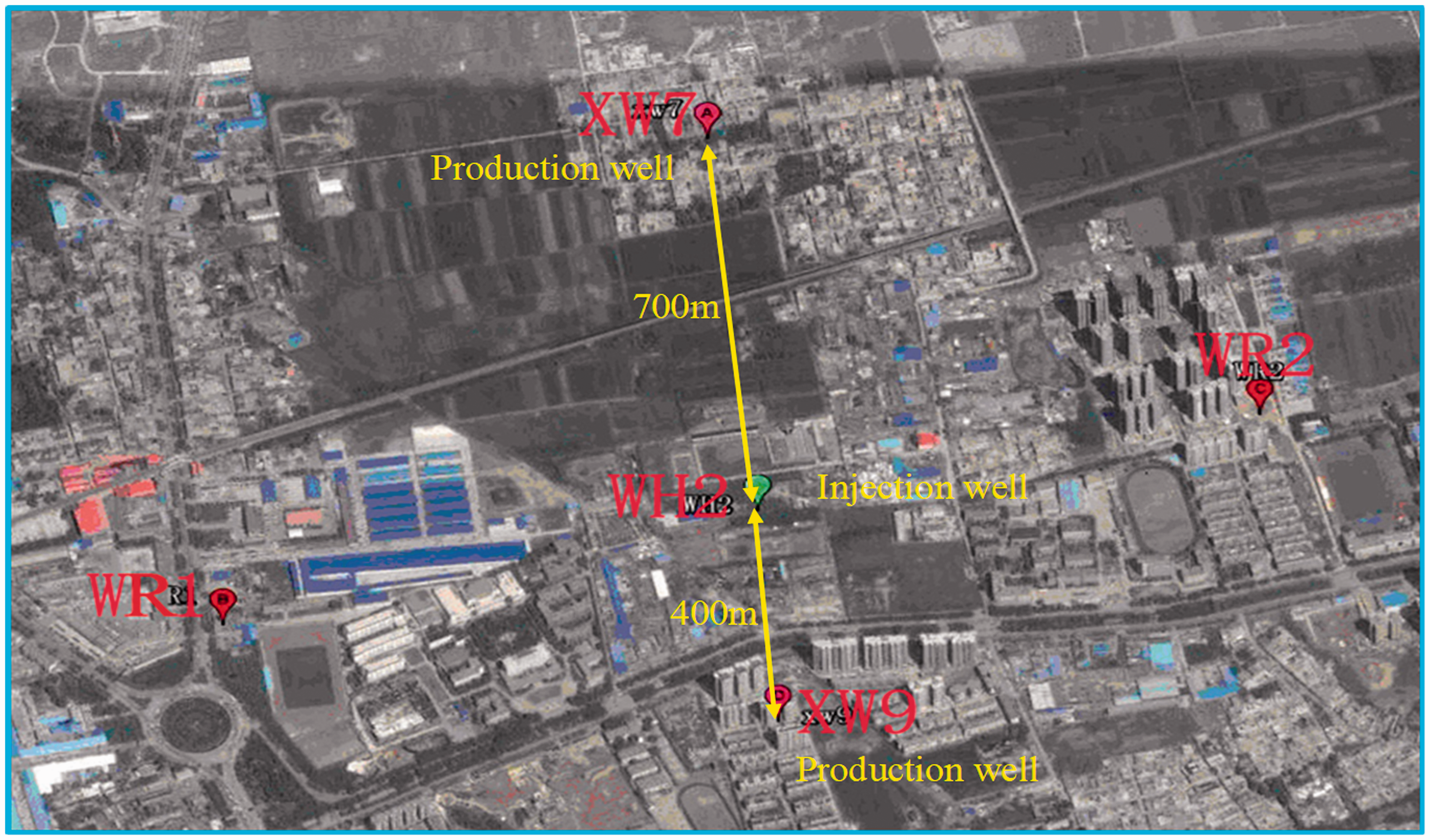
The IPWS location in Xianyang City, Shaanxi Province, China.

Hydrogeological setting

A thermal reservoir is located beneath Xianyang city, and the depth is between –1415.6 and –2656.5 m (relative coordinates are used, assuming that the surface height is zero). The reservoir rocks are classified into two rock units from the bottom to the top: a coarse sand unit and a medium-coarse sand unit. These two main units can be further subdivided depending on their lithological properties, which are particularly important for hydraulic–thermal–mechanical modeling.

The simulation area was located in the Weihe River’s first terrace region (Figure 1), which was formed from an unconsolidated aquifer resulting from deposition, where the production and injection wells belong to the same level and are closely spaced. According to the locations of the production, injection and observation wells, we know that each well was situated within a similar lithology with small variations between two neighboring rocks. Therefore, the rocks throughout the study area could be summarized as horizontally extensive. Since the strainers in the production and injection wells were placed only in shallow confined aquifers beneath –1415.6 m, the simulations mainly involved the hydraulic distribution of the confined aquifer. That is, the rocks above –1415.6 m could be summarized as an aquitard. In addition, the lithologies under –1415.6 m were mostly coarse and medium-coarse sand that formed the aquifer. However, there were clay and silt layers below –2656.5 m, and thus, it should also be considered an aquitard. Above all, there were four layers in the vertical direction. The total depth of the simulation was –3000 m. An aquitard consisting primarily of the Sanmen and Zhangjiapo groups constituted the depths from 0 to –1415.6 m. The first shallow confined aquifer ranged from –1415.6 to –2656.5 m and mainly comprised the Lantian Bahe and Gaoling groups. Another aquitard, mainly consisting of the mainly Jianxintong group, ranged from –2656.5 to –3000 m. Finally, the aquifuge was below –3000 m (Table 1).

Table 1.

Hydrogeological parameters of press-bearing aquifer.

Parameter name	Meaning	Parameter values
h	Depth of press-bearing aquifer (m)	1415–2656
K_x	Horizontal hydraulic conductivity of the aquifer layers (m/day)	5
K_y	Longitudinal hydraulic conductivity of the aquifer layers (m/day)	5
K_z	Vertical hydraulic conductivity of the aquifer layers (m/day)	0.5
S_y	Specific yield	0.26
S_s	Storage coefficient	le-5
K_d	Distribution coefficient (L/mg)	0.00003
D	Dispersity (m)	10
n	Effective porosity	0.15
$Φ$	Total porosity	0.35
R	Recharge intensity (mm/year)	15
ET	Evapotranspiration	0
$H_{k}$	Evaporation critical depth (m)	0
Q7	Well XW7 production (m³/day)	4450
T7	Well XW7 Temperature (°C)	76
H7	Water head (m)	412
Q9	Well XW9 production (m³/day)	2890
T9	Well XW9 Temperature (°C)	59
H9	Water head (m)	390

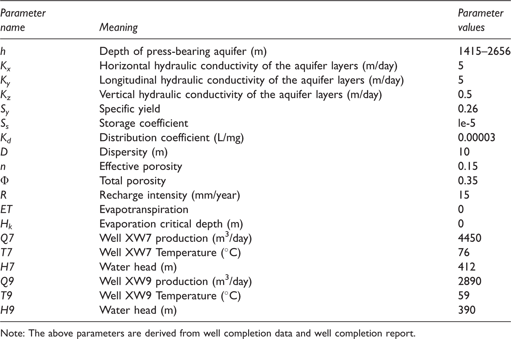
Note: The above parameters are derived from well completion data and well completion report.

This research included two experiments: production-injection and reinjection temperature measurement tests. In the first test, five wells work at the same time and the temperature field is checked. In the second test, the distance between one well and the reinjection well is adjusted under the premise of five wells working at the same time, and the method of solving the optimum well spacing is explored. There were five wells in the middle of the study area (Figure 1). Well XW7 was located at a surface distance of 700 m from WH2, and XW9 was located at a surface distance of 400 m from WH2 (Figure 1). During the two tests, well XW7 was the production well with a production rate of 4450 m³/day, a temperature of 76°C, an elevation of 442 m and a water head at 412 m. Meanwhile, well XW9 was also a production well with a production rate of 2890 m³/day, a temperature of 59°C, an elevation of 416 m, a water head at 390 m and a depth of 1600 m (Table 1). In addition, the production wells were WR1 and WR2, whose rates were 4540 m³/day and 3888 m³/day with temperatures of 66°C and 67°C, respectively. In contrast, well WH2 was an injection well with an altitude of 422 m, a depth of 2700 m, a reinjection water temperature of 36°C and a designed recharge rate of 2890 m³/day. Moreover, the temperature of the geothermal water was 75°C at the outlets of the production wells with a constant formation temperature zone of approximately 15°C. In general, the heat capacity changes with the temperature. In this paper, in order to simplify the calculation, we use the average heat capacity for the standard conditions. The average heat capacity was 4.1868 × 10³ kJ/m³, the precipitation recharge was 190 mm/year, and the running time was 120 days. A screen is installed 2000–2600 m underground for XW7 and WH2, and 1400–1500 m underground for XW9. The bottom part of the well is generally welded with a steel plate. Suitable single filtering pipe length is about 10 m and welding connections between each other in general. The slit is 10 mm (Figure 3).

We defined a model area of 2000 m along the east–west direction and 2000 m in the north–south direction. A maximum vertical extent of 3000 m was constrained by the geological boundaries, the aquitard at the top, the aquifer in the middle, and the underlying aquitard at the bottom. Both rock units were hydraulically nonconductive. Meanwhile, the aquifer was assumed to have heterogeneous and anisotropic properties. Figure 2 shows a mesh grid map of the study area, and the main parameters are shown in Table 1.

Figure 2.

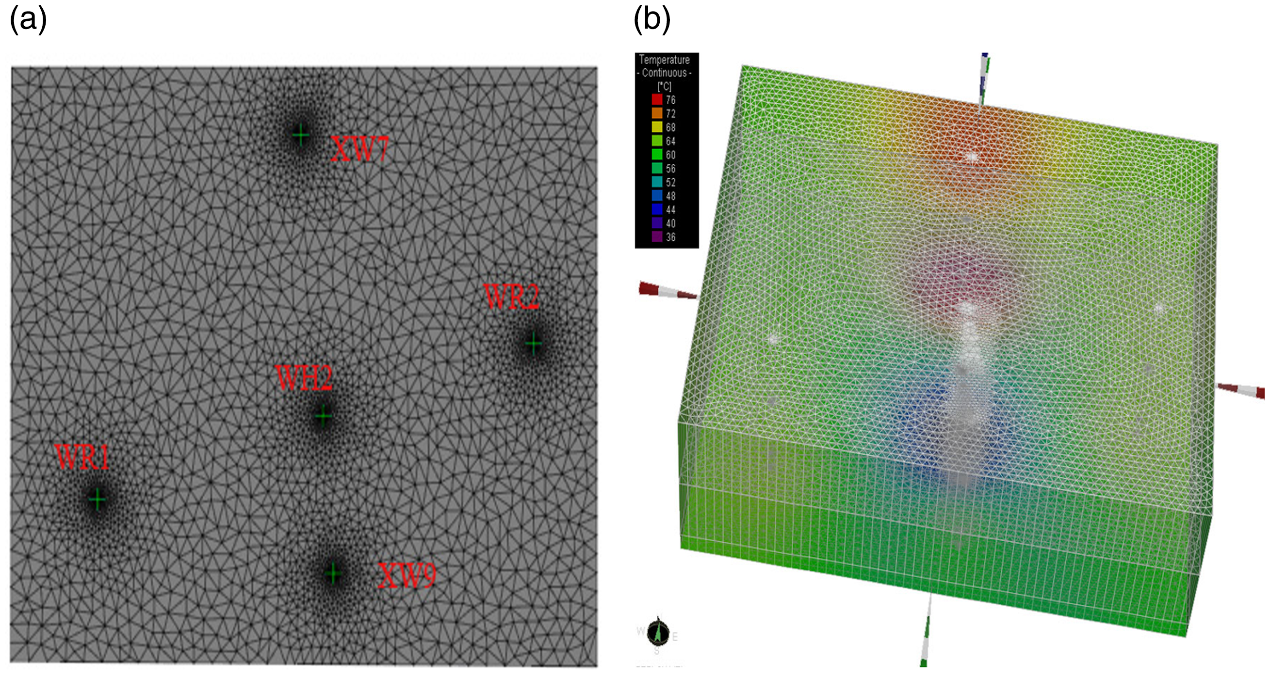
Meshing map and three-dimensional meshing. (a) Meshing map; (b) Three-dimensional meshing.

To avoid an excessive number of elements, we refined the model in the near-wellbore region and in areas of hydraulically induced fractures. Due to this refinement, the edge length of the prism front surface varied between 2.5 and 400 m in the x–y direction. To keep the ratio between the x–y and z lengths close to 1, we performed a vertical refinement by subdividing each geological layer into two sub-layers, resulting in an average thickness of 16 m. The induced fractures are represented by two-dimensional quadrilateral vertical elements. These quadrilateral vertical elements are consistent with the side surfaces of the six-node triangular prisms. Therefore, their vertical extents were 500 m, and their horizontal extent was between 2 and 3 m.

Research methods

Establishment of hydro-thermal coupling numerical model

Some researchers have conducted numerous research investigations regarding hydro-thermal coupling models for the migration of aquifer energy (Yuan et al., 2009; Zhang et al., 2006; Zhao et al., 2009). The aquifers in such models are commonly defined by a confined aquifer in terms of their level structure, heterogeneity, anisotropy, and three-dimensional unsteady flow system. Under this definition, deformation within a geological structure mainly occurs in the vertical direction and is approximately constant in the horizontal direction. When interpreting draw-down tests, pressure buildup tests, and interference or pulse tests for the pumping from deep wells, it is usually assumed that the fluid density is constant throughout the water column within the deep wells. Then, the fluid pressure values obtained at shallow depths can be directly converted into pressure values at any depth in the deep wells. In addition, the aquifer porosity is variable while assuming that the fluid density is constant.

Figure 3 demonstrates the conceptual model for the deep injection-production wells (wells XW7, XW9, and WH2, where well WH2 is a reinjection well). In addition, a seasonal alternation model can be adopted for the injection and production wells.

Figure 3.

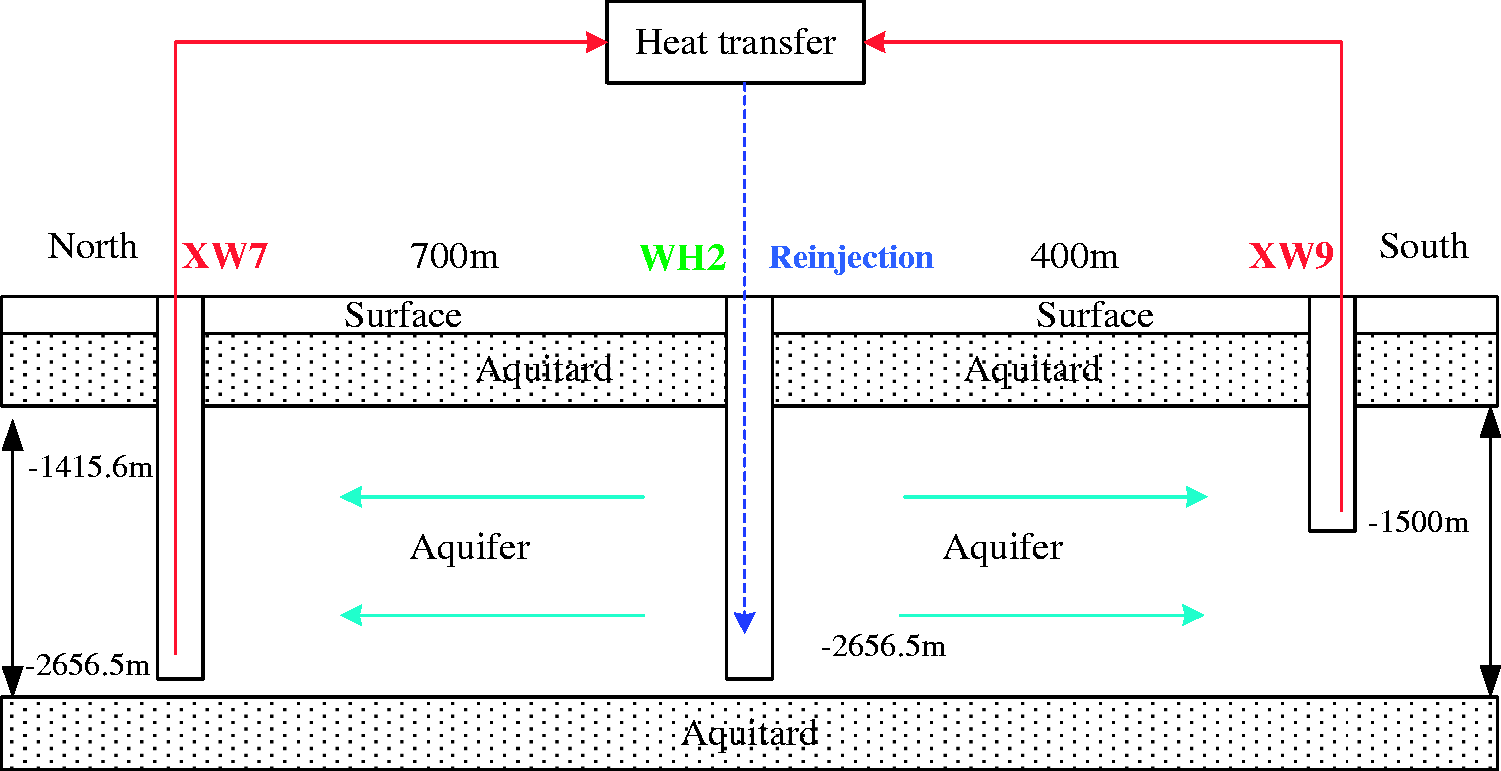
The conceptual model of injection-production wells.

Control equations

While operating the production and injection wells within a heterogeneous and anisotropic confined aquifer, the internal three-dimensional non-steady flow seepage equation and basic differential equation for thermal transport within a porous medium are as follows

μ_{s} \frac{\partial H}{\partial t} = \frac{\partial}{\partial x} (K_{x x} \frac{\partial H}{\partial x}) + \frac{\partial}{\partial y} (K_{y y} \frac{\partial H}{\partial y}) + \frac{\partial}{\partial z} (K_{z z} \frac{\partial H}{\partial z}) + w

(1)

\begin{array}{l} C_{s} \frac{\partial T}{\partial t} = \frac{\partial}{\partial x} (λ_{x x} \frac{\partial T}{\partial x}) + \frac{\partial}{\partial y} (λ_{y y} \frac{\partial T}{\partial y}) + \frac{\partial}{\partial z} (λ_{z z} \frac{\partial T}{\partial z}) \\ - C_{f} [\frac{\partial (V_{X} T)}{\partial x} + \frac{\partial (V_{y} T)}{\partial y} + \frac{\partial (V_{z} T)}{\partial z}] \end{array}

(2)

V = - K \nabla H

(3)

where

μ_{s}

: specific storage, 1/m; H: water head, m; t: time, s; K: Hydraulic conductivity, m/s; ω: source sink term;

C_{s}, C_{f}

: the specific fluid heat capacities of the porous media, J/(m³°C); T: temperature, °C; λ: dispersion coefficient, J/(m/day °C); V: seepage velocity component in spatial coordinates, m/s; n: effective porosity, %;

ρ

: fluid density, kg/m³; µ_e: elastic storage coefficient, dimensionless; K: hydraulic conductivity, m/day; M: aquifer thickness, m; and ε: vertical recharge rate, m³/(dm²) = m/day.

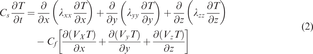
Simulation results and analysis

Assuming that the operation cycle was one year, the operation process could be divided into two stages. The first stage comprised heating for four months (2880 h), and the second stage was an intermittent period for eight months (5760 h).

Temperature simulation results in the production wells

Run from the top menu bar of FEFLOW software, a window will appear listing the available numeric engines. Although the flow model will be solved relatively quickly, the temperature simulation will take between 1 and 3 min to run to completion depending on the processor speed on your computer. To test and verify the rationality of the model simulation values, the simulated temperature results were validated using measured temperature observations. Figure 4 shows a comparison between the simulated and measured temperatures. The correlation coefficients between the simulated and measured values of these wells are greater than 0.82. Because the conditions under the ground are more complex, in this field, this value is already relatively high. It is easy to see that the temperatures among all the wells were approximately similar, which provides reliable evidence for the following analysis.

Figure 4.

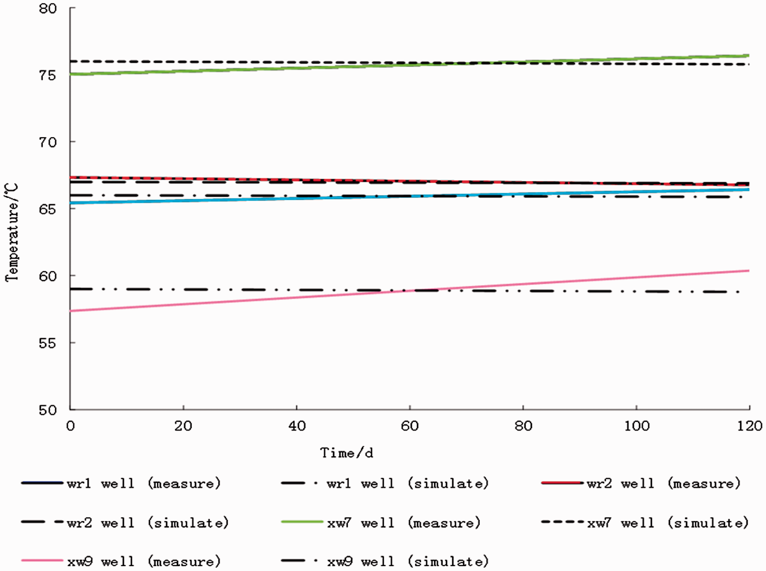
The comparison of measured and simulated results about the four production wells (WR1, WR2, XW7, and XW9).

Simulation and analysis of the flow connection

Figure 5 provides the water head various curves for the regional simulation of the performances of the production and injection wells. In production and reinjection wells, the area where groundwater pressure changes is small in the early stage of their operation, so the groundwater level changes in a smaller range. With the prolongation of pumping and recharging time, the region of pressure changes in the vicinity of pumping production and reinjection wells becomes larger (Lee, 1982). Moreover, the groundwater level changes obviously during the period of unstable pressure change (as can be seen from the diagram for one day). Furthermore, under the action of the boundary and interference effect, after about 10 days, the stable pressure drop period is reached between production and injection wells, and the change of groundwater level is very small, which means a new steady flow field occurs. However, the groundwater level at WH2 well is rising, while the groundwater levels at XW7, XW9, WR2 and WR1 wells are in a downward trend, which is consistent with the pressure variation in production and reinjection wells.

Figure 5.

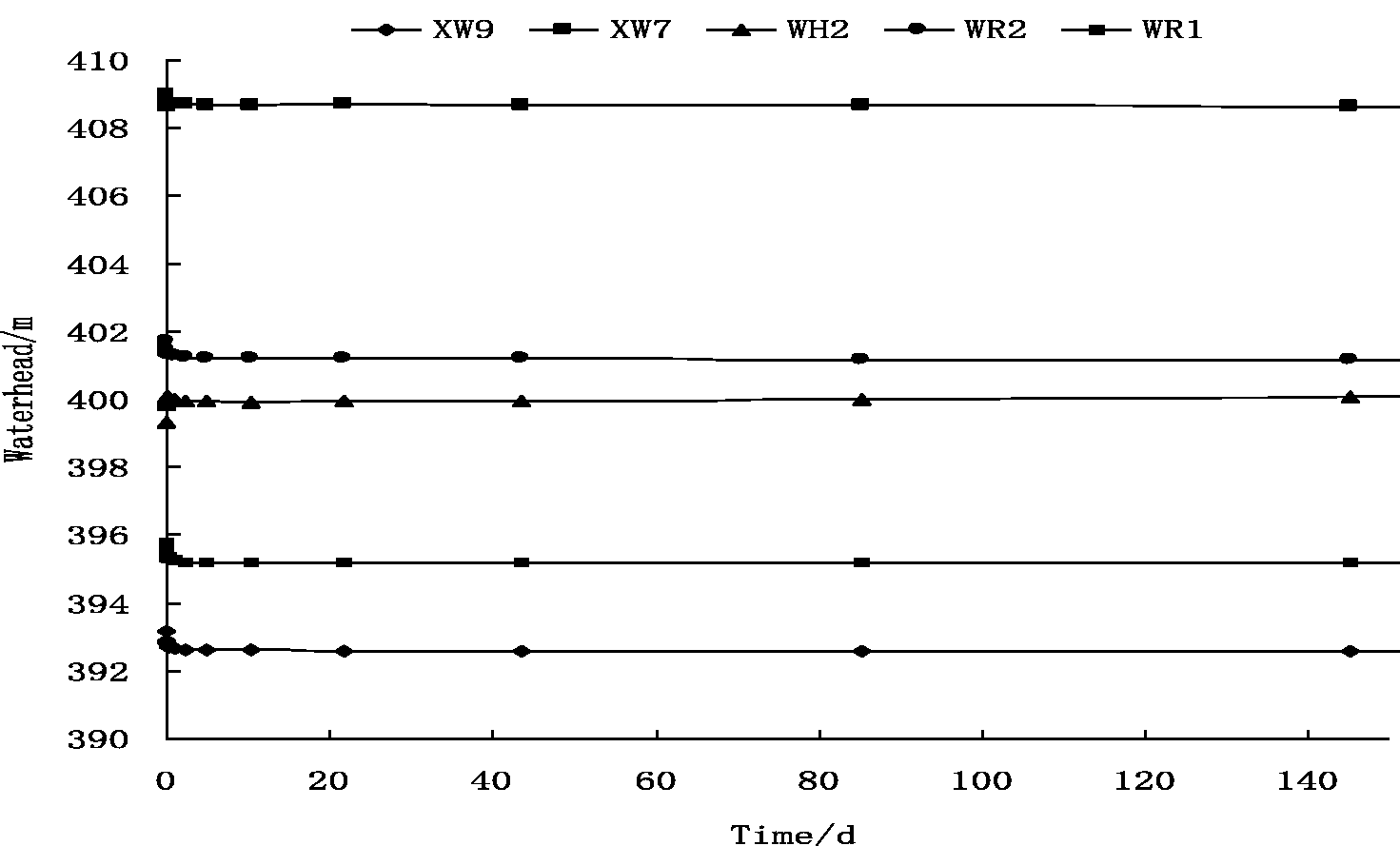
Water head varies when production and injection wells operated in simulation region.

In a word, the water pressure of the reinjection wells in the aquifer increases, while the water extracted from the aquifer around the production wells reduces the water pressure. With pumping and recharging, the area that changes pressure near the reinjection wells and production wells is expanding in the aquifer, and the water pressure difference makes the injected water flow to the production wells (Matthews and Russell, 1967). Thus, the groundwater from the reinjection water in the aquifer begins to be pumped out from the production wells, forming a new relatively stable flow field.

As the operation time increased, the hydraulic gradient value remained the same, and the energy storage laminar flow field experienced a new stabilization state, namely, a flow connection. The result here is shown in Figure 5, and we can quantitatively judge whether the flow connection occurred due to the variation of hydraulic gradient, which means the ratio of head loss and infiltration path length along infiltration path. We can also clearly observe the concept of the flow connection, which means that stable seepage occurred in the underground flow field under the forced convection between the production and the injection wells. Meanwhile, the injected water was pumped out to the production well.

Figure 6 shows the water head curves that varied with time at different distances. When the distance was 75 m and 100 m, the water head of the production well initially decreased, while the water head increased under the influence of the production well after 300 days. However, when the distance was 200 m or greater, the water head did not change over time as it was beyond the influence of the production well. Thus, it can be concluded that 200 m was the upper limit for a reasonable distance. However, this will start to change after a longer time depending on the hydraulic diffusivity term inside the independent of lactation stage (ILS) equation of radial pressure change from the production well. This situation is more complex; this article only considers the method problem, and does not consider the occurrence of this situation.

Figure 6.

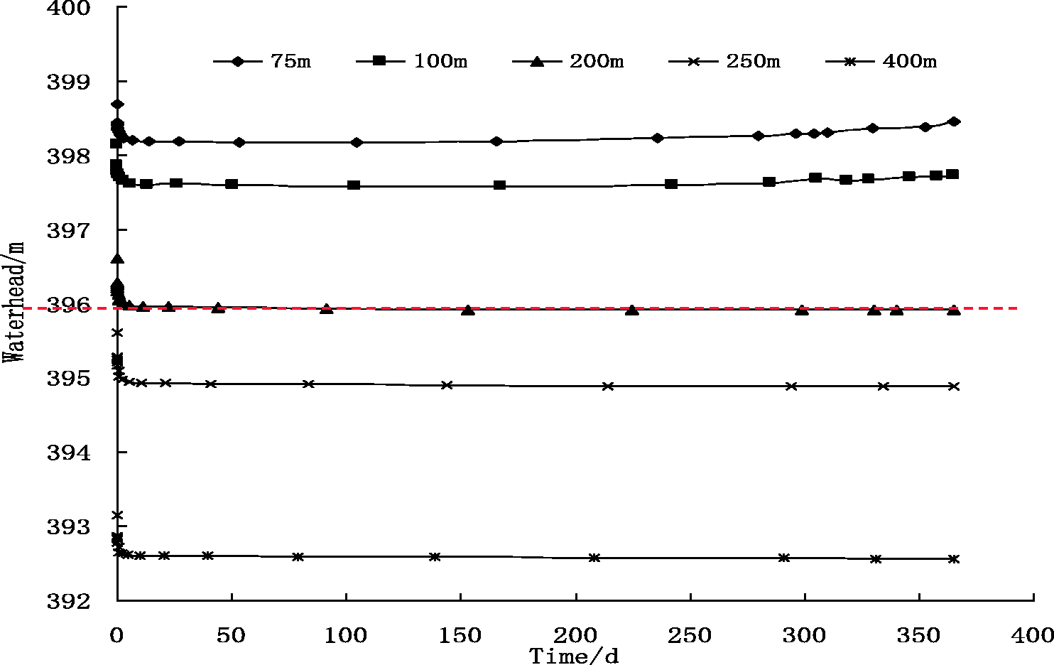
The curves of water head varied with time at different distance between production and reinjection wells.

Figure 7 shows a map of the temperature field distribution after 120 days of reinjection with an injection temperature of 36°C. From Figure 7, it is clear that the direction of the temperature field change was consistent with the direction of the groundwater flow.

Figure 7.

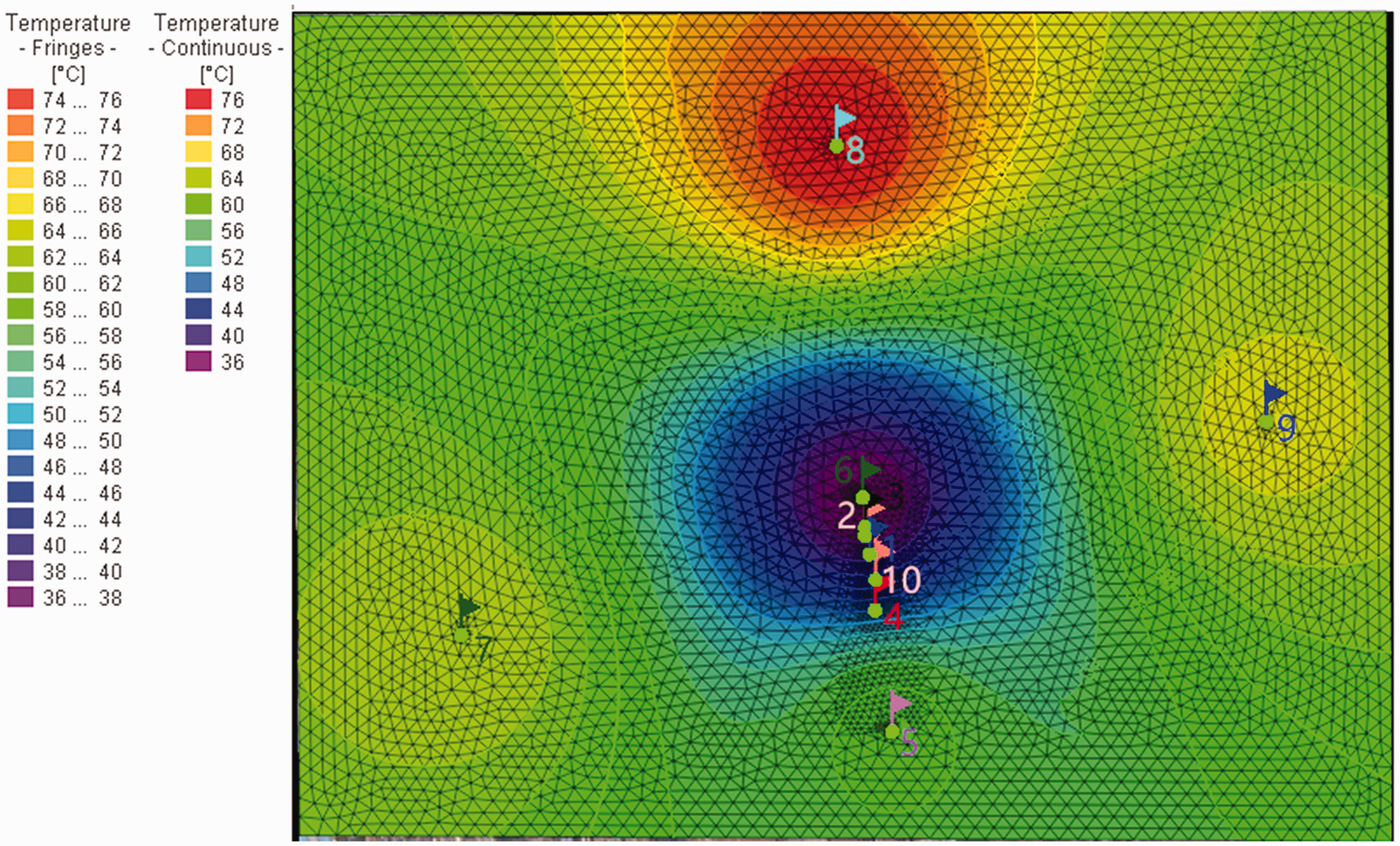
Distribution map of reinjection temperature field under the reinjection temperature being 36°C after 120 days.

By simulating the water table amplitude at different pumping volumes, it was discovered that the time required for the groundwater level to become stable changed as the pumping volume varied. To be specific, when the pumping and irrigation volumes increased, the water table evidently changed due to the influences of the pumping and injection wells. At the same time, the time constant decreased. This indicates that the time for the flow connection was shortened. The reason for this was mainly because the groundwater flow forced by convection was reinforced by the increased pumping and injecting water, which ignored the function of the natural flow field. Under such forced convection conditions, a new stable seepage flow field formed at a certain time, followed by a flow connection. This is clearly demonstrated in Figure 8, which shows the head curves varying with time for different amounts of water when the production well was 250 m away from the injection well. It is easy to see that when the pumping volume was 3000 m³/day, the time at which the groundwater formed a new steady fluid field was approximately 430 h; however, when the pumping volume was 5000 m³/day, the time decreased to approximately 190 h. This reveals that the time required to achieve a flow connection decreased with an increase in the pumping volume. Thus, knowing the water spent within an IPWS circle, the groundwater level amplitude, time constant and temperature field alteration at different distances can be simulated. In addition, the reasonable distances of the pumping and the injection wells can also be confirmed.

Figure 8.

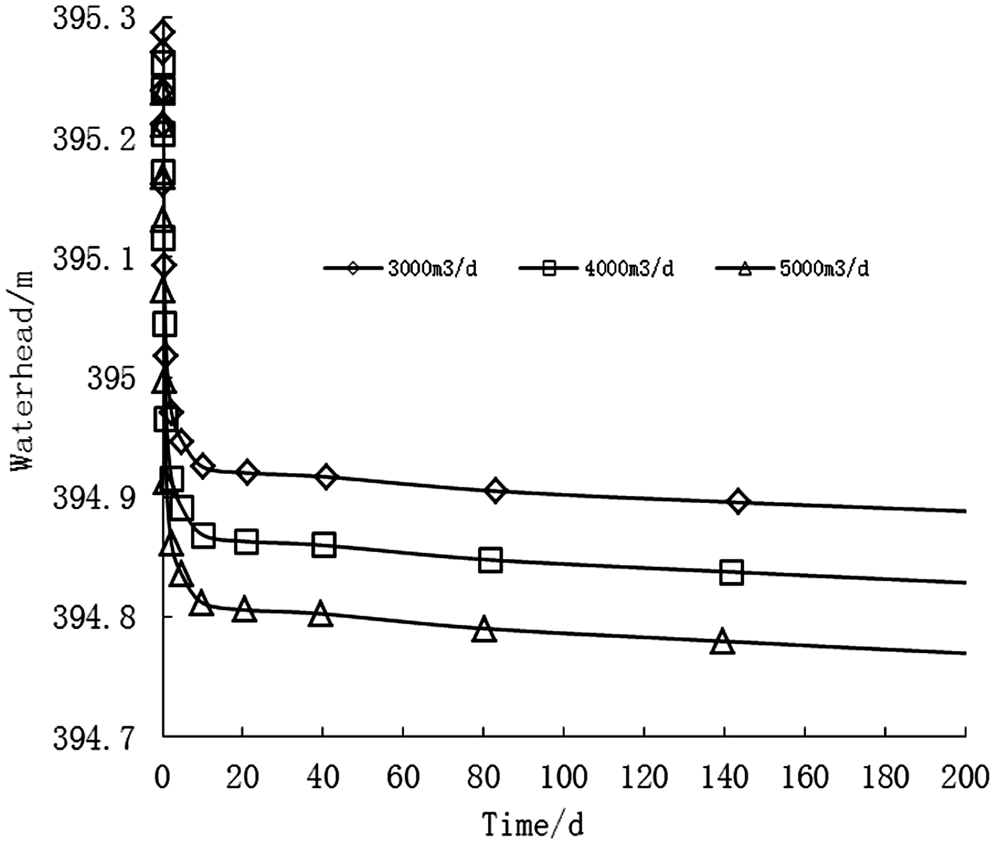
The curves of water head varying with time in different amount of water when production well was 250 m away from the injection well.

Analysis of the influence of the flow connection on the temperature field

Since the recharge water temperature was different from the original aquifer temperature, the water temperature in the injection wells was likely to make that in adjacent, production wells go up or down by a degree under heat conduction and convection processes. This phenomenon is called thermal breakthrough. To increase the influence of the temperature field in an injection well and prevent it from forming a thermal breakthrough, it is of great necessity to conduct research on the influence of the quantity of recharging water on the functional range of the temperature field.

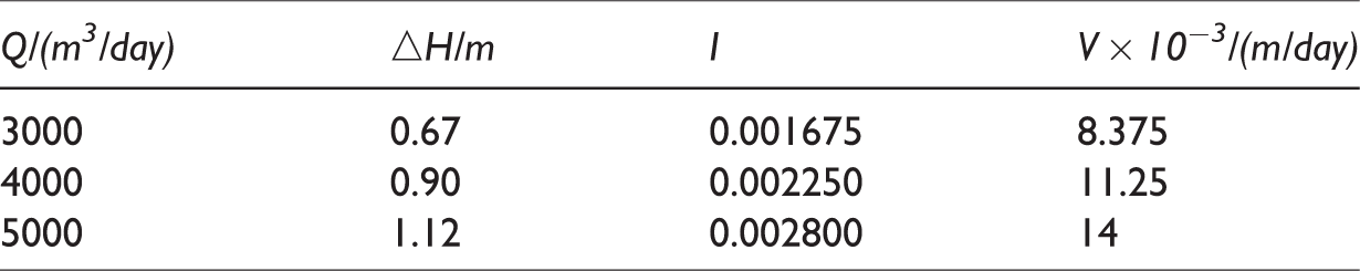
Table 2 shows the calculated average hydraulic gradient and seepage velocity of the groundwater flow for different quantities of water. Larger quantities of water recharge led to bigger hydraulic gradients and seepage flow velocities. It has been noted that when the energy abstraction system was running, the main method of heat transfer near the pumping and injection wells was convective heat transfer, the intensity of which mainly depended on the groundwater flow velocity (Zhang et al., 2006). Therefore, a larger quantity of water recharge coincided with a faster groundwater flow velocity, the convection process of heat transfer per unit time was greater, and the temperature of the production well changed faster.

Table 2.

Calculated velocities of groundwater flow under different quantity of water.

Q/(m³/day)	△H/m	I	V × 10⁻³/(m/day)
3000	0.67	0.001675	8.375
4000	0.90	0.002250	11.25
5000	1.12	0.002800	14

To better describe the range of influence of the temperature in the aquifer, it was assumed that the area within which the temperature of the aquifer increased by at least 2°C caused by recharge appeared through thermal breakthrough. Figure 9 shows the temperature curves in the production well that varied with time at seven different distances between the production and reinjection wells. Larger distances meant longer times for heat transfixion to occur. In addition, the range of the pumping temperature was smaller. When the operation time reached 120 days, the lower limit value of the reasonable distance was 180 m under the premise that thermal breakthrough would not happen. Therefore, combined with the scope of influence, it is easy to conclude that the reasonable distance was 180 m to 200 m under this study’s limited conditions. Furthermore, the optimal distance was 180 m.

Figure 9.

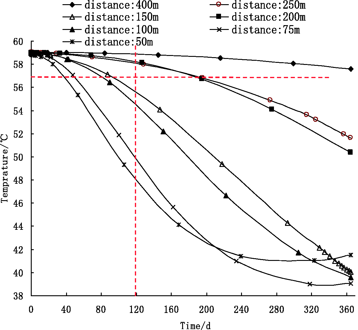
The curves of temperature in pumping well varying with time at seven different distances between the pumping and reinjection wells.

Figure 10 shows the temperature change curves with time under the different water production rates. Figure 10 shows that thermal breakthrough occurred after 360 days when the production capacity was 2890 m³/h and the well distance was 400 m. This time was later than the formation of the flow connection at 350 days under the same production and injection amounts. This demonstrates that heat transfixion only occurs after the flow connection is established and when thermal transport accompanies the flow, which could also be explained by other flow amounts. Thus, heat transfixion can be controlled through controlling the flow connection. Comparing the scopes of the influence of heat under different production and injection flows and non-production wells revealed that the thermal variation range was very small without forced convection, and the influencing range decreased as the time increased. Therefore, it can be concluded that, with an increase in the production water quantity, the variation in the water temperature in the production wells was greater, which is consistent with the above-mentioned research results.

Figure 10.

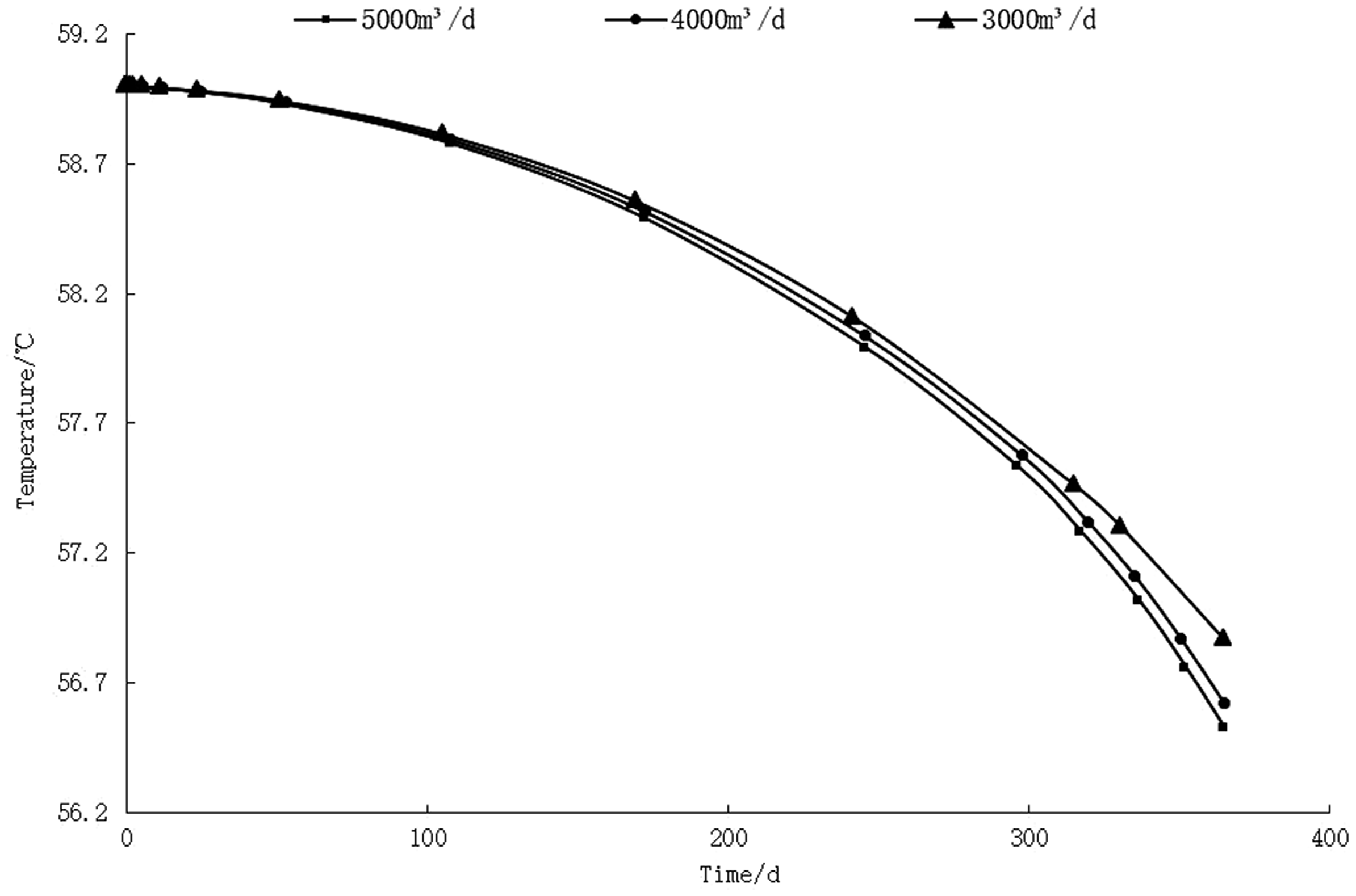
The temperature changing curves with time under the different water yielding in production wells.

On the whole, the groundwater level varies significantly with the influence of injection and production water quantity. With the increase of injection and production water quantity, the time required for the stability of the hydraulic field is reduced correspondingly. The role of the natural flow field is neglected due to the enhancement of forced convection from injection and production together. Under the influence of forced convection, a new seepage stable field is formed after a certain period of time, and when the new seepage stable field is formed, flow communication will also occur. In the fixed water quantity of injection and production conditions, different conditions of groundwater level, stable time, and temperature changes under the different wells spacing can be simulated. Then, by establishing the mutual coupling curve between the hydraulic and the temperature field, the optimum spacing between injection and production wells is determined. This method can be used as a reference for the establishment of injection and production schemes and effective management of deep underground geothermal water resources in the future.

Conclusions

Combining a numerical model of water flow fields in an underground deep aquifer with a numerical model of geothermal fields, this paper simulates the flow field and temperature field of groundwater and derives a standard to judge the flow connection using a variety of the hydraulic gradient. The main conclusions are as follows.

The coupled thermal–hydrological model is used to simulate the study area in Xianyang, Shaanxi Province, China. The results show that the model can be used to accurately and honestly simulate the distribution of the groundwater flow field and temperature field in an actual situation.

The results provide a conceptual and quantitative judgment for the critical value of the flow connection. When the hydraulic gradient is constant, a new stability state in the energy storage and laminar flow field tends to occur, namely, the critical value of the flow connection will appear.

Under a constant distance between the production and injection wells, a flow connection in the groundwater flow field is likely to occur after the IPWS have operated for a long time. In addition, with variations in the production and injection quantities, the times at which the flow communication occurs are different. Greater production and reinjection volumes lead to shorter times for flow communication.

With the hydrogeological parameters set in this paper, the most reasonable distance is 180 m to 200 m for an IPWS operation time of 120 days under the premise that thermal breakthrough will not occur and the optimum distance is 180 m between the injection and production wells.

Geothermal tail water reinjection can serve as a timely artificial recharge to the groundwater source, and reduce or prevent the formation of the falling funnel formed by the decline of the groundwater level. Therefore, in order to prevent the thermal breakthrough between injection and production wells, we need to ensure reasonable spacing and monitor it closely. In recent years, geothermal water reinjection technology has been applied only in a few fields, and only part or all of the geothermal tail water is recharged. Therefore, the ground discharge is still the most common method at present, and this technology needs to be vigorously promoted by us.

An optimal layout scheme of injection and production wells is very complex for geothermal tail water recharge, especially in the calculation of the best distance between injection and production wells. If the distance between the injection and production wells is too short, there is not enough energy exchange between the reinjection water and the dielectric skeleton, and the cool water temperature cannot rise in time, which will lead to the thermal breakthrough. If the reinjection well is too far away from the production well, the ground subsidence will be caused by excessive exploitation, with no timely restoration of groundwater. Different distances between wells may lead to different results in restoration of groundwater, so the optimal distance for reinjection is particularly important. Once an inappropriate distance is selected, it will result in irreversible consequences. Therefore, in the future, in the process of formulating new geothermal development and utilization programs, we should first complete the design of the reinjection scheme, and respond in time to the various changes of hydraulic and temperature fields caused by the development and utilization of thermal reservoirs.

Footnotes

Acknowledgements

The authors would like to acknowledge Professor Zhiyuan Ma, and graduate students: Zhihan Yun, Lei Zhen, Dan Xu and huiJv Zheng from school of Environmental Science & Engineering in helping collecting the site data, and Kara Cosentino from the University of Nebraska–Lincoln in helping correcting the English expressions.

Declaration of conflicting interests

The author(s) declared no potential conflicts of interest with respect to the research, authorship, and/or publication of this article.

Funding

The author(s) disclosed receipt of the following financial support for the research, authorship, and/or publication of this article: This work was supported by the National Natural Science Foundation of China (grants no. 41672255, 41877232, 41402255, and 41790444); High-tech research cultivation project (grant no. 300102268202); Program for Key Science and Technology Innovation Team in Shaanxi Province (grant no. 2014KCT-27), Promoting Higher Education Reform by Big Data Technology, Energizing Future Exploration in Teachers and Students (FPE, grant no: 2017B00022) and Shaanxi Provincial Institute of Higher Education 2017 Annual Higher Education Research Project (grant no: XGH17049).

References

Evans WC, Lorenson TD, Sorey ML, et al, (2014) Transport of injected isobutane by thermal groundwater in Long Valley caldera, California, USA. In: Water-Rock Interaction, Two Volume Set: Proceedings of the Eleventh International Symposium on Water-Rock Interaction, 27 June–2 July 2004, pp. 125. Saratoga Springs, New York, USA: CRC Press.

Fukuda D, Asanuma M, Hishi Y, et al. (2005) The first two-phase tracer tests at the Matsukawa vapor-dominated geothermal field, Northeast Japan. In: Proceedings world geothermal congress, pp. 24–29.

Ganguly S (2017, April) Temperature Distribution and Thermal Performance of an Aquifer Thermal Energy Storage System. In: EGU General Assembly Conference Abstracts, Vol. 19, p. 14705.

González-Vargas C, Moya-Rojas P, Sánchez-Rivera E, et al. (2005, April) Evolution of the Miravalles geothermal field in Costa Rica after ten years of exploitation. In: Proceedings world geothermal congress, pp. 24–29.

Goyal

(1999) Injection related cooling in the Unit 13 area of the Southeast Geysers, California, USA. Geothermics 28(1): 3–19.

Hawkins

Becker

Tsoflias

(2017) Evaluation of inert tracers in a bedrock fracture using ground penetrating radar and thermal sensors. Geothermics 67: 86–94.

Huo

Chen

et al . (2011) Development and testing of a remote sensing-based model for estimating groundwater levels in aeolian desert areas of China. Canadian Journal of Soil Science 91(1): 29–37.

Huo

A-D

Dang

Song

J-X

et al . (2016a) Simulation modeling for water governance in basins based on surface water and groundwater. Agricultural Water Management 174: 22–29.

Huo

Peng

Chen

et al . (2016b) Groundwater storage and depletion trends in the Loess areas of China. Environmental Earth Sciences 75(16): 1167.

10.

Jin

Huang

Tong

(2014) Remeshing‐assisted optimization for locally injective mappings. In: Computer Graphics Forum 33(5): 269–279.

11.

Kaya

Zarrouk

O'Sullivan

(2011) Reinjection in geothermal fields: A review of worldwide experience. Renewable and Sustainable Energy Reviews 15(1): 47–68.

12.

Lee

(1982) Well Testing. New York: Society of Petroleum Engineers.

13.

Huo

Liu

et al . (2013) Water resources responses to climate changes in Xi’an Heihe River Basin based on SWAT model. Journal of Water Resources Research 2: 301–308.

14.

Matthews

Russell

(1967) Pressure Buildup and Flow Tests in Wells, vol. 1. Society of petroleum engineers of AIME, Dallas, TX.

15.

Mink

Pezzopane

Culp

(2015) Small scale geothermal development – An example of cooperation between land owner and electrical cooperative. Small 19: 25.

16.

Nam

Ooka

(2010) Numerical simulation of ground heat and water transfer for groundwater heat pump system based on real-scale experiment. Energy and Buildings 42(1): 69–75.

17.

Scheiber

Ayora

Vázquez-Suñé

(2018) Quantification of proportions of different water sources in a mining operation. Science of the Total Environment 619: 587–599.

18.

Shook GM (1999, January) Prediction of thermal breakthrough from tracer tests. In: Proceedings, 24th Workshop on Geothermal Reservoir Engineering.

19.

Stefansson

V-Đ

(1997) Geothermal reinjection experience. Geothermics 26(1): 99–139.

20.

Wang

Sheng

et al . (2015) A mathematical model considering complex fractures and fractal flow for pressure transient analysis of fractured horizontal wells in unconventional reservoirs. Journal of Natural Gas Science and Engineering 23: 139–147.

21.

Wang

Gao

Jiang

et al . (2017) Analysis on thermal behavior of the type of filter tubes of extraction-injection wells in geothermal utilization. Applied Thermal Engineering 118: 233–243.

22.

Willems

Nick

Weltje

et al . (2017) An evaluation of interferences in heat production from low enthalpy geothermal doublets systems. Energy 135: 500–512.

23.

Zhang

S-Y

Q-L

et al . (2014) A coupled model simulation and application of swat-modflow based on the technology of GPR. Journal of Water Resources Research 2014: 301–308 (in Chinese, with English abstract).

24.

Yuan

Wang

Yuan

(2009) Effects of well pair distance on pumping temperature of storage exploiting in the aquifer of water-source heat pump. Building Science 25(2): 92–96 (in Chinese, with English abstract).

25.

Yuandong Z, Jiahua W and Yu L (2006) Simulation of changes in geo-temperature field due to energy abstraction from underground aquifers. Journal of Tianjin University 39(8): 907–912 (in Chinese, with English abstract).

26.

Zhao

Yan

Shao

et al . (2009) Impact of pumping and injection modes on groundwater temperature in energy extraction area with regional flow. Journal of Hunan University of Science &Technology 2(24): 24–27 (in Chinese, with English abstract).

Simulation research on the reinjection temperature fields of deep geothermal wells based on real-scale experiment

Abstract

Keywords

Introduction

Study setting

The study area

Hydrogeological setting

Research methods

Establishment of hydro-thermal coupling numerical model

Control equations

Simulation results and analysis

Temperature simulation results in the production wells

Simulation and analysis of the flow connection

Analysis of the influence of the flow connection on the temperature field

Conclusions

Footnotes

Acknowledgements

Declaration of conflicting interests

Funding

References