Sage Journals: Discover world-class research

Abstract

The process of water–gas displacement in water–drive gas reservoirs has been always an important research topic. However, knowledge about the flow patterns of water–gas flow under different conditions is insufficient at present. To investigate the variation of the geometry and position of the water–gas interface as well as the water flooding efficiency with time during water–gas displacement, the distribution law of water and gas at the microcosmic scale is simulated and analysed based on the geometric model of a single pore channel abstracted from the parallel tube bundle model and continuous tube bundle model of a porous medium reservoir, with the help of laminar two-phase flow and the level set module of COMSOL Multiphysics. The simulation results show the following: (1) Under the combined effects of the boundary layer effect, interfacial tension and pore diameter changes in water–gas displacement, the shape of the water–gas interface changes from a tongue-shape to a U-shape, during which a series of interface shapes, including a piston shape, finger shape, W-shape and Ω-shape, are observed. In the pore channel, the area of the water phase below the pore channel axial is larger than that above the pore channel axial. (2) The pore-throat ratio has a considerable impact on the shape and location of the water–gas interface as well as the displacement efficiency. When the water–gas displacement is from a small pore-channel to a large one, the displacement efficiency increases as the pore-throat ratio decreases. On the contrary, if the water–gas displacement is from a large pore channel to a small one, the displacement efficiency increases as the pore-throat ratio increases. Numerical simulation can be used to study the shape and location of the water–gas interface as well as the displacement efficiency in pore channels with different scales of diameters.

Keywords

Water–gas displacement boundary layer effect shape and location of the water–gas interface pore-throat ratio water–gas displacement efficiency

Introduction

Numerous experiments on the mechanism of water–oil displacement and characteristics of two-phase flow on the micro-scale have previously been performed by researchers. Two dimensional methods, such as plane displacement in rock core slices and physical simulations of glass etching, and three dimensional methods, such as CT scanning of rock cores (Gao et al., 2009, 2016; Ge et al., 2012; Hou et al., 2016), are mostly used. The cost of experimental simulations of water–oil displacement is high, the operation is complex, and the accuracy of monitoring technology and the obtained images is limited. However, simulations are relatively easy to be realized at present. On the contrary, experiments of water–gas displacement based on micro-physical models are difficult to conduct for several reasons: (1) In the water–oil displacement process, the water and oil can freely flow in pore channels after the model is saturated with water and oil. At atmospheric pressure and in an open state, no outflow of oil and water will occur. However, in water–gas displacement, the gas will be released if the outlet end of the pore channel is open to the atmosphere; (2) In water–oil displacement, the colour difference of water and oil is relative large; as a result, the water–oil interface is easy to observe. On the contrary, the colour difference among water, gas and the simulated porous media is small, and the gas is always transparent. Therefore, the flow of the water–gas interface cannot be readily observed (Yu, 2005). As a result, the variation law of the geometry and location of the water–gas interface, the displacement efficiency with time and their influence factors are complicated. However, in numerical simulations, a real rock core is not used. The pore system of rock core is abstracted into a mathematical model to simulate the actual water–gas displacement process. Consequently, the numerical simulation method has the advantages of convenience and visualization in studying the dynamic changes of the water–gas phase (Liu, 2013).

At present, numerical reconstruction of the pore network model of porous media is usually conducted using two-dimensional micro CT scan images or geometric modelling methods. Based on the reconstructions, numerical simulations of water–gas flow in porous media are performed. However, the object in the above method is two-phase displacement over the whole pore network (Blunt et al., 2013; Bultreys et al., 2016; Liu and Wu, 2016; Raeini et al., 2012; Zhu, 2016). In fact, simulating the multi-phase displacement in porous media by a pore network model does not calculate the fluid flow rate on the micro-scale in the pore network, but rather describes the flow model characteristics of the known flow law under different conditions (Li and Wu, 2014; Liu, 2014). The variation law of geometry and location of the water–gas interface cannot be presented clearly by the current pore network model. Effects of influence factors of the above variation law also cannot be evaluated quantitatively. In this paper, to overcome the above existing problems, visual and quantitative investigations of flow model characteristics of the water–gas interface in the pore channel are conducted by numerical simulation based on the level set method.

Tube bundle models are widely used to study water flooding models. The typical tube bundle model can be divided into two categories, the parallel tube bundle model (Figure 1(a)) and the continuous tube bundle model (Figure 1(b)). In the parallel tube bundle model, the diameter of one tube in the bundle is constant along the flow direction, whereas in the continuous tube bundle model, the tube diameter varies periodically and randomly along the flow direction.

Figure 1.

The tube bundle models. (a) The parallel tube bundle model (Bartley and Ruth, 2001); (b) The continuous tube bundle model (Yang, 2009).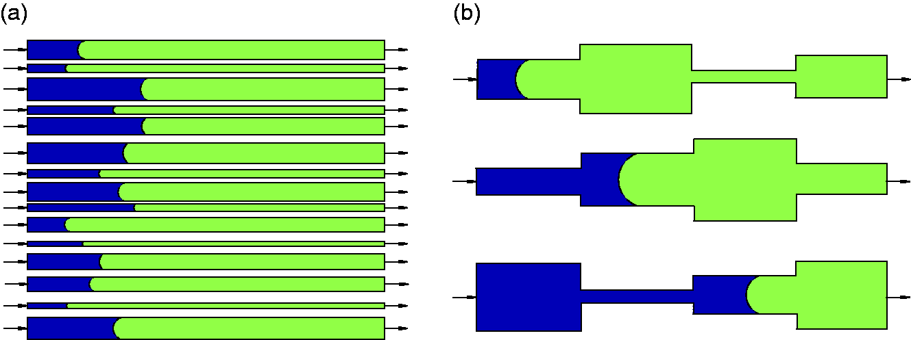

The level set method was first proposed by Osher and Sethian. It is a numerical simulation method that can be used to solve two-phase flow with surface tension (Osher and Sethian, 1988). Three two-dimensional microscopic pore models are abstracted in this work based on the elements of the parallel tube bundle and the continuous tube bundle model. Then, the geometry and location of water–gas interface are traced on the basis of the Navier–Stokes equation and the level set method. Meanwhile, the dynamic impact process of the pore-throat ratio on the geometry and location of water–gas interface and the water flooding efficiency are studied with the single factor analysis method.

Numerical simulation of water–gas displacement in the pore channel

Geometric model

The parallel tube bundle model can be regarded as a special continuous tube bundle, the pore-throat ratio of which is 1. In fact, the pore structure of porous media is closer to the continuous tube bundle model. Therefore, studying the water–gas displacement in the continuous tube bundle model is more reasonable. It can be seen from the continuous tube bundle model that in the fluid movement direction, an increase or decrease in diameter of the pore channel may occur (Figure 2).

Figure 2.

The compositions of the bundle models.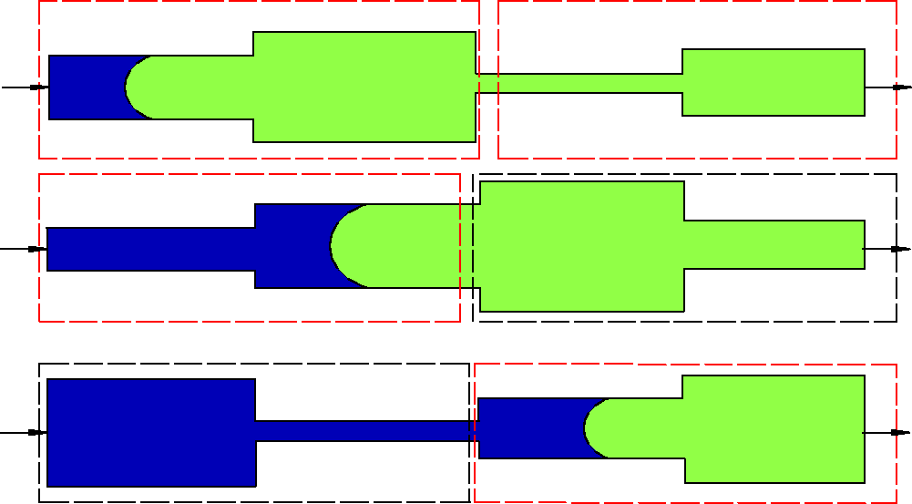

To study the two-phase water–gas displacement law in a single pore channel, the single pore channel in the parallel tube bundle model of porous reservoir is abstracted into geometric model I (Figure 3(a)). The single pore channel in the continuous tube bundle model is abstracted into model II (Figure 3(b)) and model III (Figure 3(c)). Any pore channel in the continuous tube bundle model can be considered as the combination of models II and III.

Figure 3.

The geometric models and their size. (a) Geometric mode I; (b) Geometric model II; (c) Geometric model III.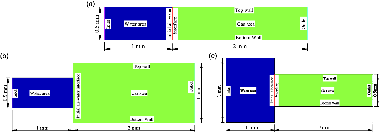

The size of the model must be determined in quantitative studies. According to the pore diameter of oil and gas reservoirs, the oil and gas can be classified as oil and gas in millimetre-pores (the pore diameter is larger than 1 mm), micrometre-pores (the pore diameter is between 1 µm to 1 mm) and nanometre-pores (the pore diameter is smaller than 1 µm). The oil and gas in millimetre and micrometre pores include conventional oil and gas that exist in structural traps, lithologic and stratigraphic traps and fractures or cavities of carbonate, and unconventional oil and gas, such as shallow biogenic gas, natural gas hydrates and heavy oil. The above analysis reveals that the order of the pore diameter of the water displacing gas reservoir is between 1 mm and 1 µm (Yang, 2015). The geometric model established in this paper is used to study the variation law of the geometry and location of the water–gas interface and the displacement efficiency. Therefore, a certain movement distance for fluids must be ensured. The order of the pore length is also an important parameter. If the orders of the length and pore diameter of the channel model are all one micron, the order of the pore length must be 100 to 1000 times the order of the pore diameter to ensure the movement distance of the fluid. Otherwise, the movement distance of fluids is not sufficiently long and the time of the water–gas displacement has a magnitude of a nanosecond, which is not convenient for data acquisition. If the order of the pore channel diameter is a micrometre and the order of the pore channel length is a millimetre, the difference between the pore channel length and diameter is one to three orders of magnitude. The larger the difference between the order of the pore channel length and diameter, the less harmonious the length-to-width ratio is. The actual scale of the pore channel in a geostatistical reservoir, the movement distance of a fluid and the harmony of the model are balanced on the basis of the scale of micro- and meso-pore model established by references (Gao et al., 2016; Liu, 2011); the determined size of model in this work is shown in Figure 3.

Basic assumptions

The framework is rigid with no deformation.

The water and gas flow is laminar.

The water phase and gas phase are immiscible.

The temperature of the seepage field is constant. The heat exchange between fluid and fluid, fluid and rock strata are in balance.

The gravity and interfacial tension are taken into consideration.

The governing equation

Using the modules of the laminar flow of two phase flow and the level set method of COMSOL Multiphysics software, the mathematical model is set up. The level set transport equation and the mass and momentum transfer equation are used in the mathematical model.

(1) Level set transport equation

The level set transport equation is used to track the change of the interface between immiscible two-phase flow (Sethian, 2003). In the level set equation, the gas area is expressed by $φ = 0$ , the water area is expressed by $φ = 1$ , and the contour lines of level set is expressed by $φ = 0.5$ . The level set equation can be seen as the volume percentage of water in the gas-liquid two-phase flow. Therefore, the migration equation of the gas–liquid interface can be written as follows (Comsol, 2015)

\begin{matrix} \frac{\partial φ}{\partial t} + u \cdot \nabla φ = γ \nabla \cdot (ɛ \nabla φ - φ (1 - φ) \frac{\nabla φ}{| \nabla φ |}) \end{matrix}

(1)

where φ is the contour line of the interface of the gas-liquid two-phase flow; γ is the reinitialization parameter to solve the equation; u is the speed of the fluid; ɛ is the thickness of the gas–liquid interface; t is the time of the gas–liquid two-phase flow.

To avoid the instability of the numerical calculation, the physical property parameters, such as the density and viscosity of the fluid near the interface, need to be processed smoothly. The smoothing process of the level set equation involves sing the level set function to express the change in the density and viscosity of fluid during the process of the gas–liquid two-phase flow; the corresponding equation is written as follows

ρ (φ) = ρ_{g} + (ρ_{w} - ρ_{g}) φ

(2)

μ (φ) = μ_{g} + (μ_{w} - μ_{g}) φ

(3)

where

ρ_{w}

is the density of water, kg/m³;

ρ_{g}

is the density of gas, kg/m³;

μ_{w}

is the viscosity of water,

Pa \cdot s

;

μ_{g}

is the viscosity of gas,

Pa \cdot s

(2) Mass and momentum transfer equation

The Navier–Stokes equation is used to describe the transmission properties of fluid mass and momentum. Because of the gas and liquid flow in the pore channel, the capillary effect must be considered in the model. Therefore, the water–gas interfacial tension is introduced into the model. In the fixed Eulerian coordinates, the revised universal Navier–Stokes equation of the two-phase flow, including interfacial tension, gravity and the two-phase interface, can be described as follows (Comsol, 2015; Roger, 1979)

\begin{matrix} {\begin{matrix} ρ \frac{\partial u}{\partial t} + ρ (u \cdot \nabla) u = \nabla \cdot [- pI + μ (\nabla u + (\nabla u))^{T}] + F_{st} + ρ g \\ \nabla \cdot u = 0 \end{matrix} \end{matrix}

(4)

where ρ is density, kg/m³; u is the velocity, m/s; I is the unit matrix; p is the inlet pressure, Pa; μ is the dynamic viscosity; F_st is the surface tension of the gas–liquid, N/m; g is the acceleration of gravity, m/s².

The surface tension can be calculated by the following the formula (Roger, 1979)

F_{st} = \nabla \cdot T

(5)

T = σ (I - ({nn}^{T})) δ

(6)

where

σ

is the coefficient of the surface tension; n is the normal vector of the interface; δ is the Dirichlet function, whose value is zero in the region outside the two-phase interface.

δ = 6 | φ (1 - φ) | | \nabla φ |

(7)

The mathematical expression of the vector of the interface is written as

n = \frac{(\nabla φ)}{| \nabla φ |}

(8)

With the finite element method used to solve the equation, the equations should be deformed firstly, and then are integrated by parts in the computational domain. To demonstrate the interaction force between the wall and fluid of the two-phase laminar flow, the boundary integral should be added into the computational domain; the formula can be written as follows (Roger, 1979)

\int_{\partial Ω} test (u) \cdot [σ (n_{wall} - (n cos θ)) δ] d S

(9)

where

θ

is the contact angle of the wall. When the no-slip wall condition is used, that is under the non-wetting condition, the boundary integral item is removed. This is because test(u) is zero on the border, and it is therefore impossible to set the contact angle. However, if the subtle boundary slip of the fluid is allowed, it is possible to set the contact angle. The additional boundary condition is given by equation (9) so that the contact angle of the wall of the two-phase fluid can be set.

Boundary condition

The velocity of the inlet and the pressure of the outlet are both set by the model. The wall of the pore channel is defined as the closed boundary and is wettable. The interface of the gas–liquid at time zero is set as the initial interface. The velocity vertical to the wall is zero. That is to say,

(1) The condition of the inlet velocity is $v_{inlet} = v (t)$ and

\begin{matrix} v (t) = {\begin{matrix} v_{0} cos (t) & 0 \leq t \leq 10^{3} μ s \\ 0 & t > 10^{3} μ s \end{matrix} \end{matrix}

(10)

(2) The condition of the outlet pressure is

{p_{outlet} = p}_{0}, n \cdot μ (\nabla u + (\nabla u)^{T}) = 0

(11)

(3) The condition of the wall is

F_{rf} = - \frac{μ}{β} u

(12)

where β is the length of the slip, whose size is equal to the size of the subdivided mesh at the boundary; F _rf is the interaction of the wall.

Initial parameters and solution setup

The physical property parameters of the numerical simulation of the water–drive gas are shown in Table 1.

Table 1.

The parameters of the numerical simulation.

Symbol	Physical parameter	Value	Unit
$ρ_{w}$	Density of water	1000	kg/m³
$μ_{w}$	Dynamic viscosity of the water	0.001	$Pa \cdot s$
$ρ_{g}$	Density of the gas	0.716	kg/m³
$μ_{g}$	Dynamic viscosity of the gas	$1.08 \times 10^{- 5}$	$Pa \cdot s$
T	Temperature	293	K
γ	Water–gas interfacial tension	50	mN/m
$p_{in}$	Gas pressure	0.1	MPa
p ₀	Outlet pressure	0.1	MPa
v ₀	Initial velocity	1	m/s
θ	Water–gas contact angle	30	°

The migration rule of the water–drive gas interface in the pore channel

The migration rule of the water–drive gas interface in the full pore

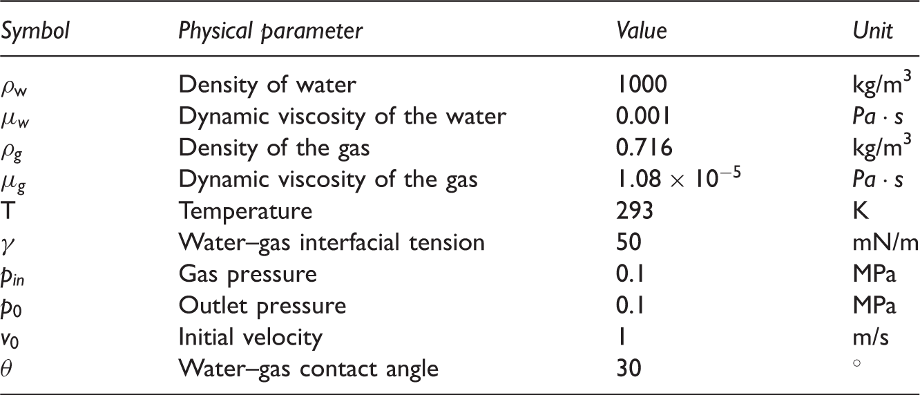
The shape change of the water–gas interface with time

Under the action of the initial rate of displacement, the change of the shape and position of the water–gas interface in the full pore with time is shown in Figure 4. The blue region is represented as the water, and the green region is represented as the gas, and the initial water–gas interface of time is zero (Figure 4(a)). During the process of the water–drive gas, the water–gas interface is obviously presented as tongue-shaped, which can be seen in Figure 4(b) to (f). After 1000 µs (1000 µs later), the speed of the water at the inlet is set as zero. Under the common action of the inertia of the water and interfacial tension, the water–gas interface continues to move forward. At 1400 µs, the interface of the water–gas is presented as U-shaped and is characterized by the capillary effect, as is shown in Figure 4(g). From then on, the interface of water–gas continues moving forward as a U-shape concave interface, which is shown in Figure 4(h). At 2200 μs, the whole region of pore is occupied by water, as shown in Figure 4(i).

Figure 4.

The shape and position of the water–gas interface through time.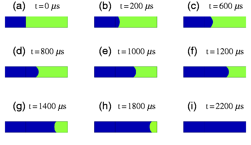

Due to the interaction between rock and fluid in the pore channel, a boundary layer with a certain thickness is produced, which results in the boundary layer effect in the pore channel. From the microscopic view, the attraction of rock molecules to fluid molecules becomes stronger the closer distance to the wall of the pore channel. The boundary layer fluid is closest to the wall of pore channel. As a result, the attraction between rock molecules and boundary fluid molecules is the strongest. Therefore, the molecules of boundary layer fluid are orderly distributed on the wall of pore channel. From the macroscopic view, viscosity is a property of fluid. The closer distance to the wall of pore channel, the larger fluid viscosity. When a fluid with a certain velocity flows in the pore channel, the boundary layer with a certain thickness is generated near the wall. Along the flow direction, the boundary layer expands to the direction of the pore axis. The distribution of the velocity at the cross-sectional area, as shown in Figure 5, is characterized by the distribution of the typical laminar flow velocity, which is the reason the water–gas interface is tongue-shaped and continues moving forward in the first 1200 μs (Lin, 2013).

Figure 5.

The flow velocity of the laminar flow.

Due to the contact angle of 30 degrees, which is under 90 degrees, the rock mass is wettable; that is to say, the rock mass is hydrophilic. The wettability of the pore channel can make the liquid spread effectively on the wall of the pore channel. When the fluid moves forward along the wall of the pore channel under the action of the interfacial tension, the horizontal speed of the water near the wall is greater than that near the axis of the pore channel. After the velocity of the water at the inlet is set to zero, the action of the interfacial tension emerges. With the action of the interfacial tension, the velocity of the fluid near the scope of the upper and lower wall is greater than that near the axis of the pore channel. This causes the water–gas interface near the wall to surpass that of the water–gas interface near the axis of the pore channel. The above dynamic process can be seen in Figure 4, as the tongue-shaped water–gas interface (Figure 4(f)) dynamically changes to a U-shape concave interface (Figure 4(h)).

The change of area percentage of water–gas two-phase fluid with time

The water flowing in the pore channel drives the gas forward. The percentage of water area increases while the percentage of gas area decreases. The percentages of water and gas area are shown in Figure 6. It can be seen from Figure 6 that the percentage of water area (47.2%) and that of gas area (52.8%) are nearly equal at the time of 1000 μs. The whole pore channel is occupied completely by water. During the time period of 0–2200 μs, the water area and gas area exhibit a linear increase and a linear decrease, respectively. At 2200 μs, the whole gas region is fully occupied by water.

Figure 6.

The change of areal percentage of the water–gas two-phase fluid with time.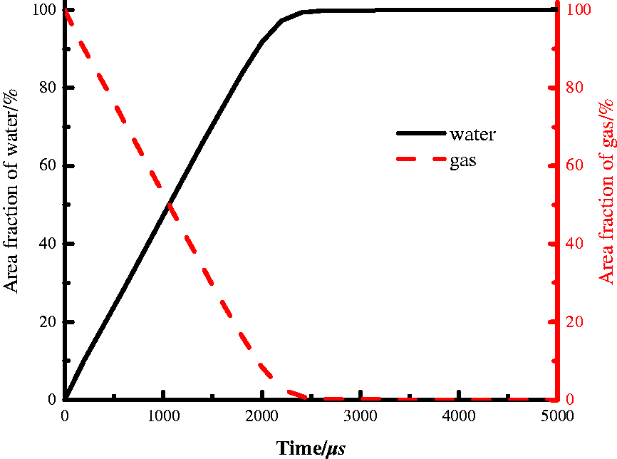

The migration rule of the water–drive gas interface from the small pore channel to the large pore channel

The change in shape of the water–gas interface with time

The change in the shape of the gas–drive-water interface from a small pore channel to a large pore channel with time is shown in Figure 7. The water–gas interface at time 200, 600 and 800 μs demonstrates an obvious tongued advance, which is illustrated in Figure 7(b) to (d). At time 1000 μs, the water–gas interface begins showing signs of a piston-like shape, but the whole water–gas interface is represented as an Ω-shape (Figure 7(e)). After 1000 μs, the velocity of the inlet becomes zero. The water–gas interface continues to move forward under the coaction of the inertia of water and interfacial tension. During the period of time of 1000–2000 μs, the water–gas interface is presented as an Ω-shape, of which the middle is high and both sides are short (Figure 7(f)). At time 3000 μs, the water–gas interface appears as a W-shape, of which both sides are long and the middle is short, as shown in Figure 7(g). At time 3200 μs, the water–gas interface near the upper and lower wall surpass that near the axis of the pore channel and is represented as a U-shape concave interface, which is characterized by the capillary effect (Figure 7(h)). By 4600 μs, the whole pore channel is occupied by the water, as shown in Figure 7(i).

Figure 7.

The shape of the water–gas interface through time.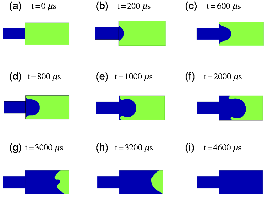

During the water–driving-gas process from a small pore channel to a large one, the boundary layer effect occurs under the action of the velocity of the fluid at the inlet. With the action of the boundary layer, the position of the water–gas interface near the axis moves ahead of that near the upper and lower wall. Therefore, an Ω-shape of the water–gas interface is presented. Simultaneously, the wettability of the hydrophilic rock mass makes the wall of the pore channel wet. Under the action of the interfacial tension, water flows along the wall of the pore channel, as demonstrated in Figure 7(b) to (f). Due to the existence of the initial rate of displacement at the inlet, the interfacial tension has weak action on the shape of the water–gas near the wall of the pore channel. After the rate of displacement becomes zero, the action of the interfacial tension of the hydrophilic rock mass begins to show up gradually. The important manifestation of the action of the interfacial tension is that the migration velocity of the water–gas interface near the wall of the pore channel is greater than that near the axis of the pore channel. This phenomenon can explain the lagging water–gas interface near the wall of the pore channel surpassing the advancing water–gas interface near the axis of the pore channel. It is also the reason for the U-shape concave interface characterized by the capillary effect.

The change of the water–gas interface position with time

It can be seen from Figure 7 that during the process of the water–drive-gas, the water area under the axis of the pore channel is larger than that above the axis of the pore channel. That is to say, the water area is asymmetrical to the axis of the pore channel. The asymmetry of the water area can be verified by the asymmetry of the contact point between the water–gas interface and the upper and lower walls of the pore channel. Figure 8(a) shows that the asymmetry of the upper and lower contact points becomes increasingly more obvious after 1000 μs. This is because the action of gravity is considered in the Navier–Stokes equation. Before the velocity of the water reaches zero, the coaction of the interfacial tension and gravity on the asymmetric behaves relatively weakly. After the velocity reaches zero, the effect of the coaction of interfacial tension and gravity on the asymmetry becomes obvious. The asymmetry also exists during the water–drive-gas process in the full pore, which is shown in Figure 8(b).

Figure 8.

The contact point between water–gas interface and the pore channel wall. (a) Two-phase displacement from the large pore channel to the small pore channel; (b) Two-phase displacement in the equal-diameter pore channel.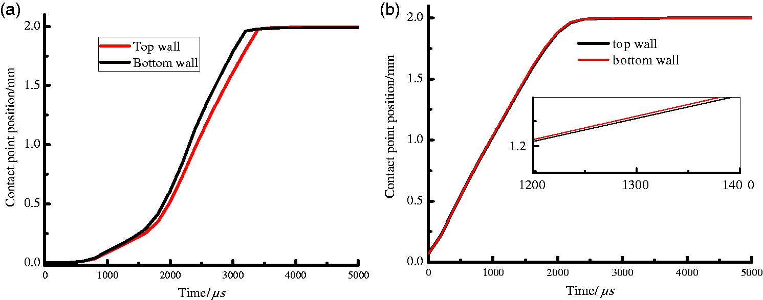

When water drives gas from the small pore channel to the large pore channel, the coaction of the displacing velocity and gravity makes the weight of the water under the axis of the pore channel greater than that above the axis of the pore channel. After the displacing velocity reaches zero, the water–gas interface moves forward along the horizontal direction under the coaction of interfacial tension and the inertia of the water. Because the weight of the water under the axis of the pore channel is higher than that above the axis, the inertia of the former is greater than the latter. Therefore, in the same time period, the position of the water–gas interface under the axis of the pore channel is ahead of that above.

The change in the areal percentages of gas and water with time

It can be observed from Figure 9 that the ratio of the gas area to the water area is 4 at 1000 μs. At 2000 μs, the gas area is nearly equal to the water area. The whole pore channel is occupied by water at 4600 μs. In contrasting Figure 9 with Figure 6, the gas area and water area exhibit non-linear changes when the fluid flows from the small pore channel to the large pore channel. The larger the diameter of the pore channel is, the larger the initial gas area is. The velocity of water at the inlet of the equal-diameter pore of model I and the unequal-diameter pore of model II is the same. Therefore, the same weight of water enters into the pore channel at the same time. To the same length of the pore channel, it takes longer to occupy the gas region in the large diameter pore channel of model II than in the equal-diameter pore channel of model I.

Figure 9.

The area fraction of gas and water at different time.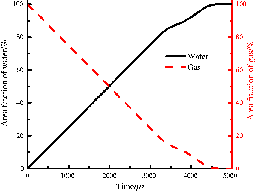

The migration rule of the water–drive gas interface from the large pore channel to the small pore channel

The change in shape of the water–gas interface with time

During the water–drive gas process from the large pore channel to the small pore channel, the shape of the water–gas interface changes with time, as shown in Figure 10. The initial water–gas interface at time 0 is shown in Figure 10(a). The water–gas interface of time 200 μs is presented as tongue-shaped, which is shown in Figure 10(b). At time 400, 600, 800 and 1000 μs, the water–gas interfaces are all presented as finger-shaped, as shown in Figure 10(c) to (f). The water–gas interfaces of time 1200 and 1600 μs are presented as a U-shape concave interface, which can be observed from Figure 10(g) and (h). The whole pore channel is occupied by water at time 2000 μs, as is shown in Figure 10(i).

Figure 10.

The shape of the water–gas interface through time.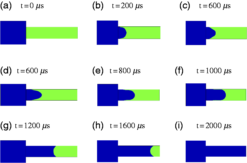

During the water–drive gas process from the large pore channel to the small pore channel, because the dynamic viscosity of water is 100 times that of gas, the water deviates from steady state flow to some extent and the water–gas interface deforms. The water presented as a finger-shape drives gas; this phenomenon is also known as Saffman–Tayloy fingering, and it is shown in Figure 11 (Brailovsky et al., 2006; Kang, 2004; Li and Sander, 1987; Saffman and Taylor, 1988). In fact, the Ω-shape of the water–gas interface during the water–drive gas process from the small pore channel to the large pore channel can also be considered as an example of Saffman–Tayloy fingering.

Figure 11.

The schematic of the shape of fingering (Brailovsky et al., 2006; Kang, 2004; Li and Sander, 1987; Saffman and Taylor, 1988).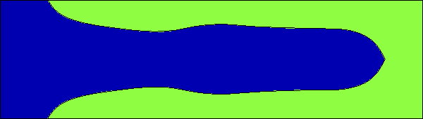

The position changes of the water–gas interface with time

During the water–drive gas process from the large pore channel to the small pore channel, the water area under the axis of the pore channel is greater than that above. That is to say, similar to the rule of the water–drive gas process for the equal-diameter pore channel and from the small pore channel to the large pore channel, asymmetry of the water area also exists about the axis of the pore channel exists during the water–drive gas process from the large pore channel to the small pore channel. The asymmetry can also be presented by the difference of the horizontal position of the contact point between the water–gas interface and the upper and lower walls of the pore channel, as is shown in Figure 12. However, the difference of asymmetry of model III is weaker than that of model II. This is because the inlet velocity of model II and model III is the same, and simultaneously, the weight of the water entering into the pore channel of model III is greater than that of model II. After the velocity reaches zero, the inertia of water in model III is greater than that in model II.

Figure 12.

The change curve of the position of the contact point between the water–gas interface and wall.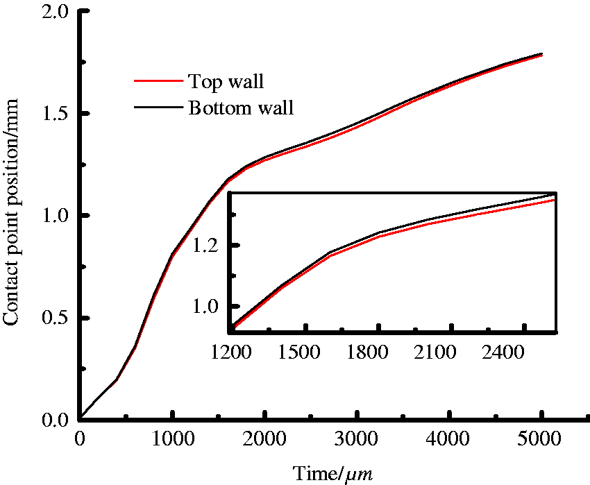

The change of the area fraction of water and gas with time

In the water–drive gas process from the large pore channel to the small pore channel, the change curve of the area fraction of water and gas with time is shown in Figure 13. At time 500 μs, the water area is nearly equal to the gas area. By 2000 μs, the whole pore channel is occupied by water. In the first 1000 μs, the area fraction of water increases linearly with time, but the area fraction of gas decreases linearly.

Figure 13.

The area fraction of water and gas through time.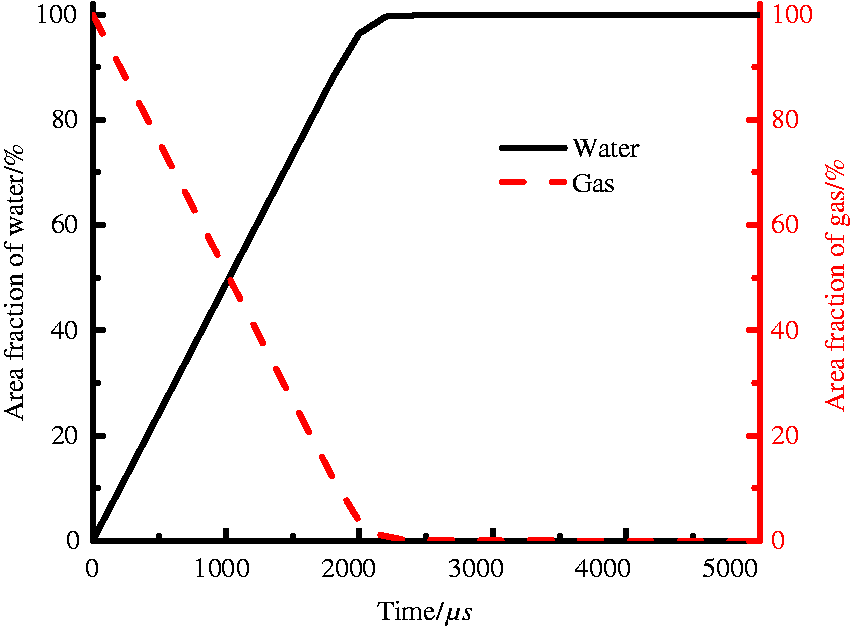

The initial gas area of the model II and model I is same at time 0 μs. Contrasting Figure 6 with Figure 13, the growth rate of water area fraction in model III is greater than that in model I. This is because the velocity of the inlet in the both models is same, but the flow section of the large pore channel is greater than that of the small pore channel. Therefore, in the same time period, the weight of the water entering into the model III is larger than that entering into the model I, which results in the efficiency of displacement in model III is higher than that in model I.

The effect of pore-throat ratio on the migration rule of water–drive gas interface

The effect of pore-throat ratio on the migration rule of the water–drive gas interface from the small pore channel to the large pore channel

The effect of pore-throat ratio on the shape of the water–gas interface

For the water–drive gas process from the small pore channel to the large pore channel, the water–gas interfaces and positions of five different pore-throat ratios of 1, 2, 4, 5 and 10 at time 200, 1000 and 5000 μs are shown in Figure 14. The figure shows (1) at 200 μs, the water–gas interface is tongue-shaped. The smaller the pore-throat ratio is, the larger the region of water is. (2) At 1000 μs, the water–gas interface moves forward along the axis of the pore channel in the Ω-shape. (3) After the inlet velocity reaches zero, the water drives the gas in the pore channel under the coaction of gravity, interfacial tension and inertia. At 5000 μs, the whole pore channel is occupied by water for pore-throat ratios of 1 and 2, whereas the water and gas regions coexist in the pore channel for pore-throat ratios of 4, 5 and 10. For the pore channels with pore ratios of 4, 5 and 10, the higher the pore-ratio is, the smaller the area of water is, the larger the gas area is, and significant differences in terms of the water–gas interface shape exist. It can be concluded that when the cross-sectional area of the pore channel transitions from small to large, different degrees of cross-sectional area changes can lead to differences in the shape of the water–gas interfaces. Moreover, with the continuous migration of the water–gas interface, the shape of the water–gas interface will have a great effect on the water–drive gas efficiency under different pore-throat ratios.

Figure 14.

The shape of the water–gas interface of different pore-throat ratios at 200, 1000 and 5000 μs.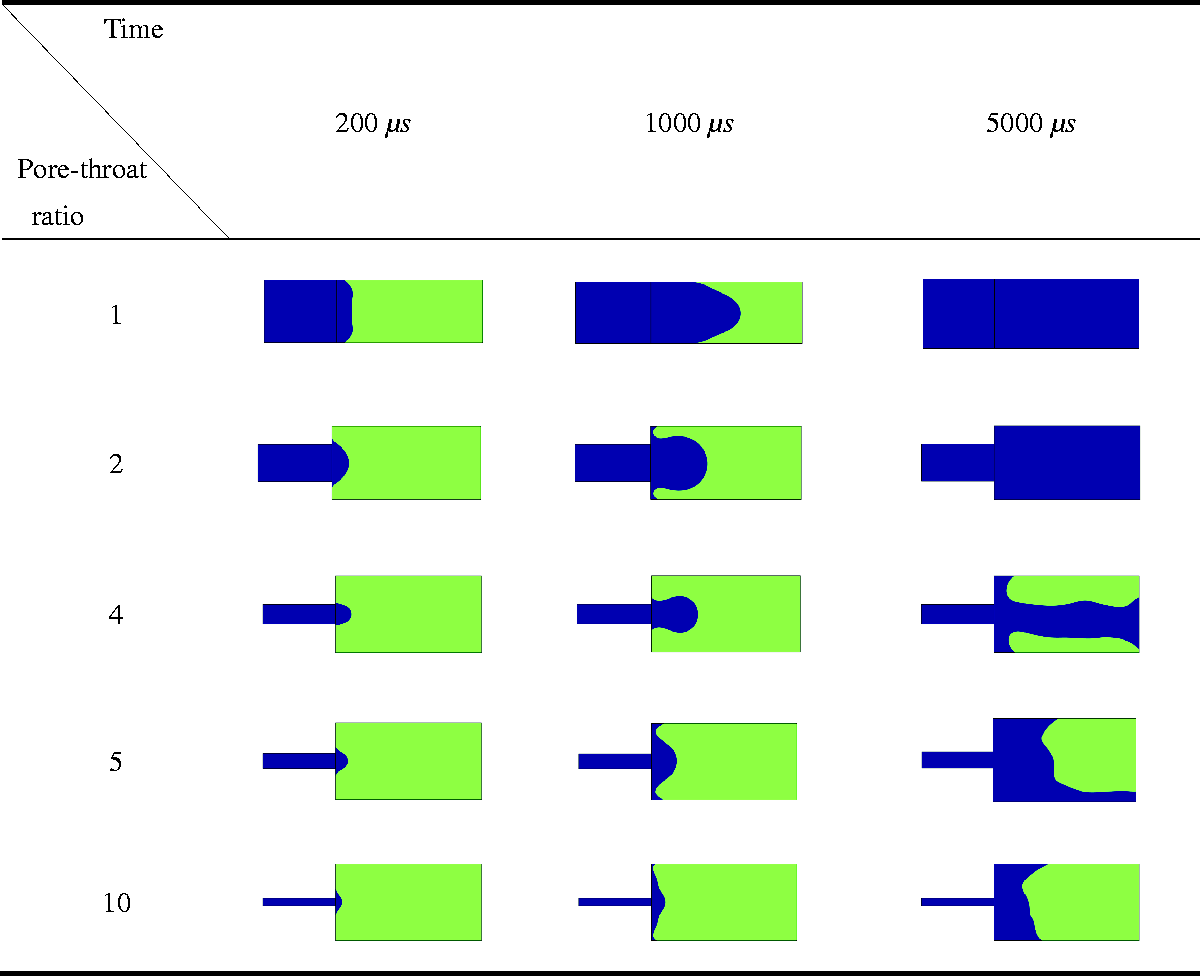

The effect of the pore-throat ration on the areal fraction of the water

In the water–drive gas process from the small pore channel to the large pore channel, the changing curve of the areal fraction of water in the pore channel with different pore-throat ratios of 1, 2, 4, 5 and 10 over time is shown in Figure 15. At 2000 μs, the areal fractions of water with different pore-throat ratios of 1, 2, 4, 5 and 10 are 95.8%, 50.3%, 24.5%, 20.1% and 10.0%, respectively, and 99.9%, 99.9%, 49.4%, 48.5% and 25.7%, respectively, at 5000 μs. It is shown that the areal fraction of water decreases obviously with the increase of the pore-throat ratio. That is because when the water and gas flows in the small pore channel, the height of the water–gas interface is nearly equal to the diameter of the small pore channel. After the water flows into the large pore channel from the small pore channel, the water–gas interface continues moving forward at the original height. The larger the pore-throat ratio is, the greater the difference between the large pore channel and the small pore channel is. As a result, the area of gas left within a certain range of the upper and lower wall of the pore channel with a large diameter increases. Therefore, during the water–drive gas process from the small pore channel to the large pore channel, the efficiency with a large pore-throat ratio is low, whereas the efficiency with a small pore-throat ratio is high.

Figure 15.

The areal fraction change of water with different pore-throat ratios through time.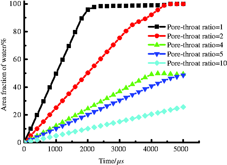

The effect of pore-throat ratio on the migration rule of the water–drive gas interface from the large pore channel to the small pore channel

The effect of pore-throat ratio on the water–gas interface shape

In the water–drive gas process from the large pore channel to the small pore channel, the shape and position of the water–gas interface with five different pore-throat ratios of 1, 2, 4, 5 and 10 are shown at time 200, 600 and 1000 μs in Figure 16. As is can be observed from Figure 16, (1) the water–gas interfaces are all tongue-shaped at 200, 600 and 1000 μs, and the larger the pore-throat ratio is, the farther the water–gas interface in the small pore channel is. (2) At time 1000 μs, the pore channel for pore-throat ratios of 5 and 10 is fully occupied by water, but the gas region and water region coexist in the pore channel with pore-throat ratios of 1, 2 and 4. The smaller the pore-throat ratio is, the farther the water–gas interface is. It can also be concluded that when the cross-sectional area transitions from large to small, different degrees of cross-sectional area changes can yield different water–gas interface shapes. Furthermore, with the continuous migration of the water–gas interface, the shape of the water–gas interface will also have a considerable effect on the water–drive gas efficiency under different pore-throat ratios.

Figure 16.

The shape of the water–gas interface with different pore-throat ratios at 200, 600 and 1000 μs.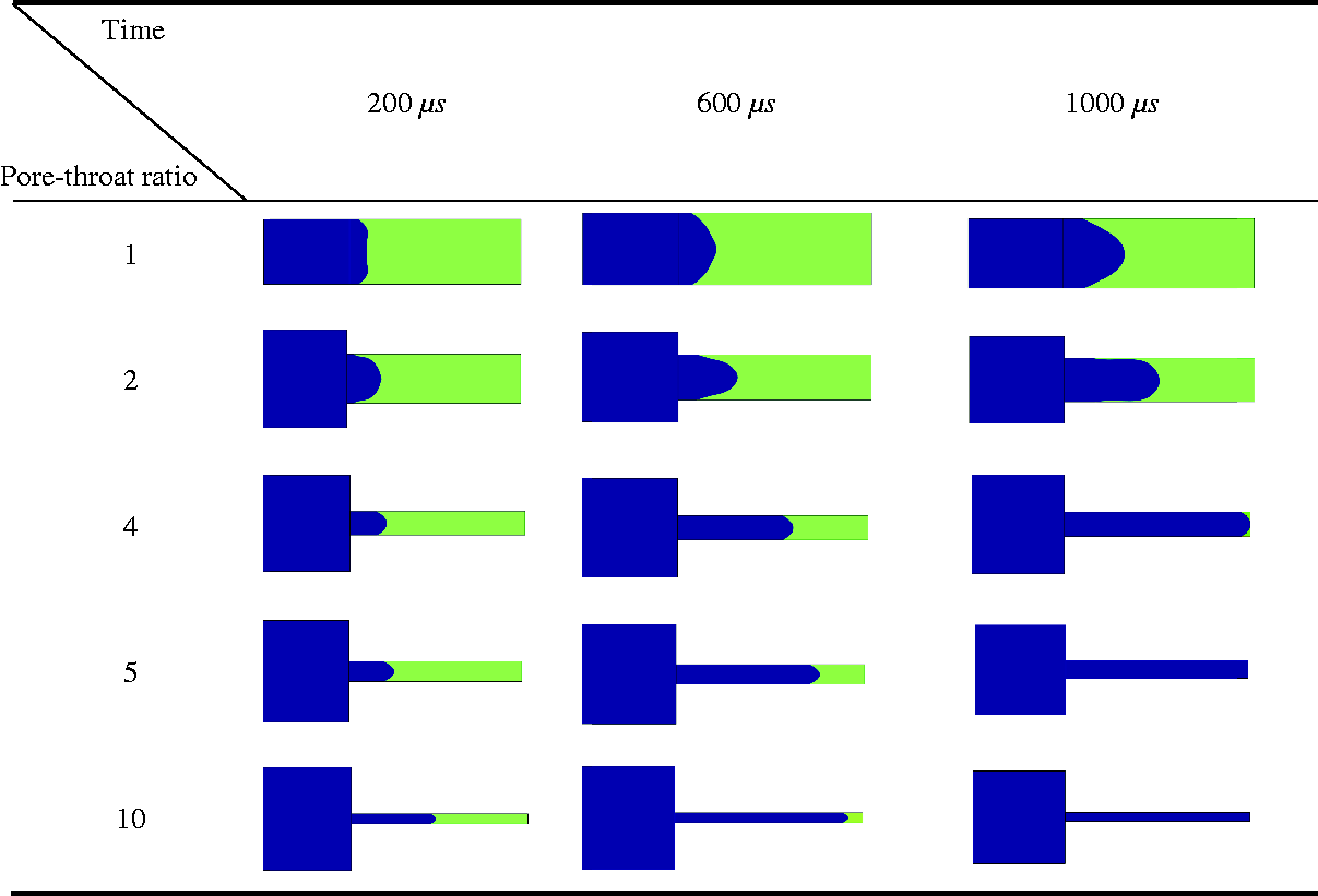

The effect of pore-throat ratio on the areal fraction of the water

In the water–drive gas process from the large pore channel to the small pore channel, the changing curve of the areal fraction of water with different pore-throat ratios of 1, 2, 4, 5 and 10 over time is shown in Figure 17. It can be observed from Figure 17 that when water drives gas from the small pore channel to the large pore channel, the larger the pore-throat ratio is, the shorter time it takes to occupy the gas region with water. This is because the inlet velocity is the same, and the quality of water flowing into the small pore channel is also equal. The larger the pore-throat ratio is, the smaller the diameter of the small pore channel is. Therefore, the water–drive gas efficiency is higher if the water flows farther into the small pore channel.

Figure 17.

The change in the areal fraction of water with different pore-throat ratios through time.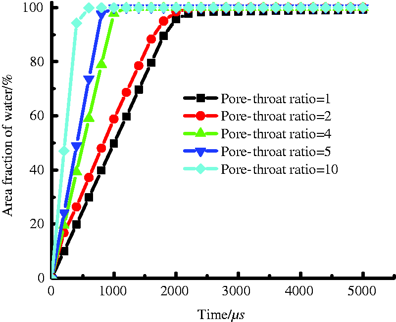

Conclusions

The boundary layer effect, interfacial tension and size of the pore channel have substantial effects on the shape of the water–gas interface. With changes in the displacing velocity, the shape of the water–gas interface experiences a process of change from a tongue-shaped to a concave U-shaped interface, with a series of transition interface shapes, such as an Ω shape, W shape, piston-like shape and finger shape, rather than exhibiting piston-like displacement throughout the whole process. The various shapes of the water–gas interface in the pore channel are related to pore-scale, and they are also influenced by the interfacial tension, contact angle and other factors. The various shapes of the water–gas interface show the dynamic morphological change of the interface during the two-phase fluid flow in the pore channel and are dynamic change characteristics of the water–gas interface. During the water–drive gas process, the area of water is asymmetric about the axis of the pore channel. The asymmetry is mainly reflected in that the area of water under the axis of the pore channel is greater than that above, and the velocities of the contact point of water–gas interface and lower wall are greater than those of the water–gas interface and upper wall.

The pore-throat ratio is a characteristic parameter that represents the change of the pore channel diameter. And it is also an important factor for determining the capillary effect, the shape of the water–gas interface and the water–drive gas efficiency. In the water–drive gas process from a small pore channel to a large pore channel, the smaller the pore-throat ratio is, the smaller the difference is for the height of the water–gas interface and the diameter of the large pore channel, and the higher the water-flood efficiency is. On the contrary, with a greater difference in the height of the water–gas interface and the diameter of the large pore channel, the lower the water flooding efficiency is. During the water–drive gas process from the large pore channel to the small pore channel, the larger the pore-throat ratio is, the farther the water–gas interface moves, and the higher the water-flood efficiency is. Otherwise, the water–gas interface moves less and the water flooding efficiency is lower.

Footnotes

Declaration of conflicting interests

The author(s) declared no potential conflicts of interest with respect to the research, authorship, and/or publication of this article.

Funding

The author(s) disclosed receipt of the following financial support for the research, authorship and/or publication of this article: This work was supported by the National Key Research and Development Program of China (no. 2017YFC0603001), the National Science Fund for Excellent Young Scholars (no. 51522406), and the Fundamental Research Funds for the Central Universities [China University of Mining and Technology] (no.2014YC03).

References

Bartley

Ruth

(2001) Relative permeability analysis of tube bundle models, including capillary pressure. Transport in Porous Media 45(3): 447–480.

Blunt

Branko

Bijeljic

et al. (2013) Pore-scale imaging and modelling. Advances in Water Resources 51: 197–216.

Brailovsky

Babchin

Frankel

et al. (2006) Fingering instability in water–oil displacement. Transport in Porous Media 63(3): 363–380.

Bultreys

De Boever

Cnudde

(2016) Imaging and image-based fluid transport modeling at the pore scale in geological materials: A practical introduction to the current state-of-the-art. Earth-Science Reviews 155: 93–128.

COMSOL Company (2015) Capillary Filling – Level Set Method, Sweden, Stockholm: COMSOL Company, pp. 1–24.

Gao

Jiang

Wang

(2016) Simulation analysis of microscopic water–oil displacement based on Level set method. Petroleum Geology and Engineering 5: 91–96 (In Chinese).

Zhang

Jiang

et al. (2012) Study on influencing factors of chemical flooding for heavy oil. Journal of Dispersion Science and Technology 33(1–3): 278–286.

Guo

Yuan

(2009) Experimental study of microscopic water displacement in low-permeability and low-pressure reservoirs by using sandstone slice. Journal of Oil and Gas Technology 4: 100–105 (In Chinese).

Hou

Zheng

Song

et al. (2016) Three-dimensional physical simulation and optimization of water injection of a multi-well fractured-vuggy unit. Petroleum Science 13(2): 259–271 (In Chinese).

10.

Kang

Zhang

Chen

SY.

(2004) Immiscible displacement in a channel: Simulations of fingering in two dimensions. Advances in Water Resources 27(1): 13–22.

11.

(2014) Characteristics of Micro Scale Capillary Interface in Ultra-Low Permeability Reservoirs, Beijing: Petroleum Industry Press, pp. 1–150.

12.

Sander

(1987) Viscous fingers in porous media. Physical Review A 36(36): 4551–4554.

13.

Lin

(2013) Fluid Mechanics, Beijing: Tsinghua University Press, pp. 1–525 (In Chinese).

14.

Liu

Lin

Song

et al. (2013) A pore scale modelling of fluid flow in porous medium based on Navier–Stokes equation. Disaster Advances 6(1): 129–136.

15.

Liu

Zhu

Liang

(2014) Digital rock physics of sandstone based on micro-CT technology. Chinese Journal of Geophysics-Chinese Edition 57(4): 1133–1140 (In Chinese).

16.

Liu

Zhang

Guo

(2011) Micro-simulation and analysis of distribution of oil water two-phase in water-flooding reservoir. Journal of Engineering Thermophysics 2: 261–264 (In Chinese).

17.

Liu

(2016) Pore scale modeling of liquid-gas two-phase flow based on geometrical reconstruction. Journal of Engineering Thermophysics 5: 1016–1020.

18.

Osher

Sethian

(1988) Fronts propagating with curvature-dependent speed: Algorithms based on Hamilton-Jacobi formulations. Journal of Computational Physics 79(1): 12–49.

19.

Raeini

Blunt

Bijeljic

(2012) Modelling two-phase flow in porous media at the pore scale using the volume-of-fluid method. Journal of Computational Physics 231(17): 5653–5668.

20.

Roger

(1977) Navier–Stokes Equations: Theory and Numerical Analysis, New York: North-Holland Publishing Company, pp. 157–246.

21.

Saffman

Taylor

Geoffrey

(1988) The penetration of a fluid into a porous medium or Hele-Shaw cell containing a more viscous liquid. Proc R Soc A 245(1242): 155–174.

22.

Sethian

(2003) Level set methods and fast marching methods. Journal of Computing & Information Technology 11(1): 400.

23.

Yang

Currier Robert

Zhang Duan

(2009) Ensemble phase averaged equations for multiphase flows in porous media. Part 1: The bundle-of-tubes model. International Journal of Multiphase Flow 35(7): 628–639.

24.

Yang

Zou

(2015) Characteristics of nano-sized pore-throat in unconventional tight reservoir rocks and its scientific value. Journal of Shenzhen University (Science & Engineering) 3: 257–265 (In Chinese).

25.

(2005) Study on Seepage Mechanism and Simulation Theory and Method of Water Drive Gas Reservoir, Chengdu: Southwest Petroleum University, pp. 1–116 (In Chinese).

26.

Zhu

Zhou

(2016) Numerical simulation of displacement characteristics of CO₂ injected in pore-scale porous media. Journal of Rock Mechanics and Geotechnical Engineering 8(1): 87–92.

Numerical simulation of migration characteristics of the two-phase interface in water–gas displacement

Abstract

Keywords

Introduction

Numerical simulation of water–gas displacement in the pore channel

Geometric model

Basic assumptions

The governing equation

Boundary condition

Initial parameters and solution setup

The migration rule of the water–drive gas interface in the pore channel

The migration rule of the water–drive gas interface in the full pore

The shape change of the water–gas interface with time

The change of area percentage of water–gas two-phase fluid with time

The migration rule of the water–drive gas interface from the small pore channel to the large pore channel

The change in shape of the water–gas interface with time

The change of the water–gas interface position with time

The change in the areal percentages of gas and water with time

The migration rule of the water–drive gas interface from the large pore channel to the small pore channel

The change in shape of the water–gas interface with time

The position changes of the water–gas interface with time

The change of the area fraction of water and gas with time

The effect of pore-throat ratio on the migration rule of water–drive gas interface

The effect of pore-throat ratio on the migration rule of the water–drive gas interface from the small pore channel to the large pore channel

The effect of pore-throat ratio on the shape of the water–gas interface

The effect of the pore-throat ration on the areal fraction of the water

The effect of pore-throat ratio on the migration rule of the water–drive gas interface from the large pore channel to the small pore channel

The effect of pore-throat ratio on the water–gas interface shape

The effect of pore-throat ratio on the areal fraction of the water

Conclusions

Footnotes

Declaration of conflicting interests

Funding

References