Sage Journals: Discover world-class research

Abstract

The presence of default U-values in Energy Performance Certificate (EPC) databases disrupts the natural variability in measured U-value distributions. Default values, often used by assessors when empirical data is unavailable, introduce deterministic artefacts into datasets, creating artificial peaks that obscure underlying statistical patterns. This study examines the impact of these default values and identifies appropriate statistical models – Lognormal, Gamma and Normal – for measured U-values in Ireland’s national EPC dataset, comprising 463,582 dwellings. Lognormal and Gamma distributions aligned better with the central peaks, while the Normal distribution more accurately captured the tails. Although no single distribution perfectly fits the data, the Normal distribution was selected as a reasonable and interpretable approximation due to its simplicity, stable parameters, and practical advantages for modelling. This choice was validated through internal data-splitting, external comparison using an independent housing sample, and simulations of typical wall configurations. The findings highlight the distorting influence of default U-values on national modelling efforts and support the use of updated, data-driven defaults. Adopting an empirically grounded Normal distribution for measured U-values enables more robust characterisation of building stock thermal performance and supports improved interpretation of thermal energy performance in built environment policy development.

Practical Application: The research improves the accuracy of building stock energy models by identifying the Normal distribution as the best fit for measured U-values in Ireland’s EPC database. It addresses inaccuracies caused by deterministic default U-values, advocating for data-driven dynamic defaults to better represent thermal performance. The findings enable the development of statistically robust reference dwellings (RDs) and more accurate retrofit strategy planning. Validated through internal and external methods, the approach supports improved policy formulation and energy efficiency assessments. The methodology can be generalised to other regions, enhancing the accuracy of national energy models and guiding effective retrofit policies.

Keywords

Best-fit criterion U-value EPC EPC data stock modelling thermal transmittance

Highlights

(1) EPC U-values are a mix of empirical and default data, default U-values disrupt distribution associated with measured data, so do not fit standard statistical distributions

(2) Lognormal, Gamma and Normal distribution functions best fit the measured data.

(3) Normal distribution selected as a reasonable fit.

Introduction

Reducing energy use and associated greenhouse gas emissions in the residential sector requires accurate and reliable building stock energy consumption models.¹ In the EU, such models use, as an input, thermal transmittance (or U-value) data from Energy Performance Certificate (EPC) datasets.

In statistics, according to the “Central Limit Theorem” even for skewed or non-normal data, the means of sufficiently-large random samples should approximate to a normal distribution.² However in Ireland’s national residential EPC database, U-value data from 463,582 dwellings³ does not fit to any standard statistical distribution.⁴ This is because the presence of deterministic default U-values EPC databases disrupts the natural variability in measured U-value distributions.

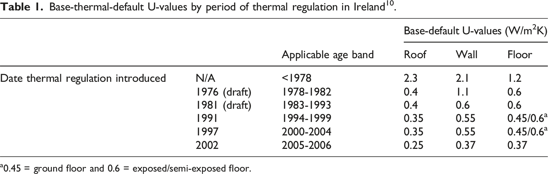
Ireland’s national EPC Dwelling Energy Assessment Procedure (DEAP) methodology requires EPC Assessors to calculate and hence enter an actual U-value into the national calculation software and national EPC dataset.⁵ If, however full details are not available, the Assessor selects a wall-type and construction period and DEAP selects a base-thermal-default U-value as shown in Table 1. Base or as-built Irish thermal default U-values (similar to many other EU member states^6,7) are determined by^8,9;

• Building element type (roof, wall or floor),

• For pre-thermal regulation dwellings (pre-1978), the date of construction,

• For post-thermal regulation dwellings (1978 – 2006), prevailing draft or finalised building codes by period of construction - allowing a grace period of generally two to three years after a proposed change in draft or finalised regulations for a dwelling to be completed.

Table 1.

Base-thermal-default U-values by period of thermal regulation in Ireland¹⁰.

		Applicable age band	Base-default U-values (W/m²K)
		Applicable age band	Roof	Wall	Floor
Date thermal regulation introduced	N/A	<1978	2.3	2.1	1.2
	1976 (draft)	1978-1982	0.4	1.1	0.6
	1981 (draft)	1983-1993	0.4	0.6	0.6
	1991	1994-1999	0.35	0.55	0.45/0.6^a
	1997	2000-2004	0.35	0.55	0.45/0.6^a
	2002	2005-2006	0.25	0.37	0.37

^a0.45 = ground floor and 0.6 = exposed/semi-exposed floor.

Default U-values thus introduce deterministic values into datasets, creating artificial peaks that misrepresent the true distribution of U-values. A 2022 study on default use within the Irish EPC dataset from 1 in 3 EPC entries to be characterised on default U-Values in 2020.¹¹ As a result, standard statistical distributions fail to model EPC U-value data accurately. This adversely affects the reliability of national building stock models, potentially leading to misinterpretations of energy performance in policy interventions. This research:

• Investigates why no standard distribution fits ‘measured’ U-value EPC field data.

• Identifies the best-fit distribution for EPC U-values.

• Validates the best-fit distribution through internal data-splitting, external validation using independent housing samples, and comparisons with simulated data.

• Improves the definition of reference dwellings (RDs) in stock energy models, ensuring that EPC-based characterisations are statistically robust and aligned with real-world building conditions.

• Refines default U-values by establishing a robust, data-driven approach to derive evolving U-values based on the 90^th percentile of their distributions, ensuring their relevance as the building stock evolves.

Background

Primary contributors to EU greenhouse gas (GHG) emissions in 2024 are transport (31%), households (27%), and industry (25%).¹² A significant share of residential emissions is attributed to the 67% of European housing stock being built prior to the widespread implementation of thermal building regulations for housing.¹³ The energy intensity of a building stock evolves over time due to changes in reference 13,

• Construction rates

• Dwelling sizes

• Specifications of newly-built homes

• Construction techniques

• Material and component types

• architectural design

• Heating systems

• Occupant behaviours and space usage

• Appliance efficiencies

• Economic conditions

• Regulatory frameworks

• Refurbishment extent and rate.

The multiple and changeable collinearities between these factors make it difficult to isolate their individual impacts on energy consumption.^14,15 Indeed, one study found that nearly half of the variability in energy use remains unexplained.¹⁴

With average replacement rates for existing housing stocks below 0.1% per year,⁵ most of today’s dwellings will still be in place in 2050.⁶ For instance, in the United Kingdom, around 75% of dwellings that will exist in 2050, were already built in 2008.⁷ Given this slow rate of stock turnover, reducing overall residential energy demand requires a combination of; (i) energy-efficient refurbishment of existing homes,^4,8–11 (ii) improvements in energy production and distribution systems, and (iii) a transition away from fossil fuel dependence.

Energy consumption in residential buildings is primarily determined by the interplay between thermophysical properties, local climate conditions,^14,16,17 and occupant behaviour.¹⁸ In the EU-27, space heating and water heating accounted for 79% of residential energy use in 2019, equivalent to 198.82 million tonnes of oil equivalent (Mtoe) or 2,242.46 TWh.^19,20 A 2009 European study²¹ of 12,500 centrally-heated dwellings across the EU identified heating system efficiency, external wall thermal transmittance, and dwelling geometry as the primary factors influencing home energy performance ratings, collectively explaining approximately 75% of the variance. Variations in heating system efficiency, primary fuel type, and heat sources contribute to differences in energy use^22,23 and carbon emissions²⁴ between otherwise similar dwellings. Some studies emphasise the role of system characteristics, such as heating system efficiency, primary fuel type, and heat source, as the most significant determinants of energy use,^22,23 while others attribute greater importance to the building fabric.^25,26 In Ireland, for the predominant dwelling type, 80% to 90% of heat loss occurs via heat transfer through the building fabric, 8% to 16% of heat is lost through air infiltration, and 4% to 16% of heat is lost through thermal bridges.^4,13

In a broadly common approach across the 30 EPC schemes in Europe and the UK,^11,27 by applying uniform assumptions about thermal properties and occupant behaviour, EPC methodologies can generate comparable energy ratings across similar dwelling types, enhancing consistency in the certification process.²⁸ These databases provide the most comprehensive data sources on the energy performance of national buildings stocks.^{1,11,13,27,29–35}

The EU Energy Performance of Buildings Directive (EPBD) requires that energy refurbishments follow cost-optimal criteria, preventing low-cost but inefficient upgrades and prioritising interventions with a strong lifecycle cost-benefit ratio.^36,37 Cost-optimality models require extensive and computationally demanding thermophysical data. The EPBD prescribes the use of reference buildings (RBs) as national building stock representatives for each EU member state.^38–40 A transparent EU-wide RB reporting framework (Regulation No 244/2012) facilitates inter-country comparisons and supports development of cost-optimal refurbishment strategies.^38,40–42 RBs are based on⁴³ high-quality auditable empirical data from statistically significant up-to-date samples. The accuracy of national building stock assessments improves with sub-categorisation of a building stock into more RB types. However, the effectiveness of this approach depends on the selection and definition of building subcategories, data validity, and default parameter choices.

Average building stock U-values characterise each RB intended to be representative of a proportion of a building stock.^4,44 A basic U-value is given by.

U = \frac{λ}{L} (W / m^{2} K)

(1)

Where;

L = thickness of material (m)

λ = thermal conductivity of material (W/mK)

Default U-values and their limitations

Where the cost of obtaining the measured data is prohibitive, EPC assessors use nationally prescribed default U-values.⁴⁵ The latter are intentionally pessimistic to 46;

• Avoid overestimating a dwelling’s energy performance,

• Highlight potential retrofit benefits to homeowners,

• Prompt assessors to obtain more detailed building data where possible.

As is standard in EPC schemes across Europe,¹¹ thermal default U-values are based on historical regulatory requirements or construction standards relevant to the building’s construction period.⁴⁰ As shown in Figure 1, thermal building regulations started to influence European dwelling U-Values in the late 1950s/early 1960s with mandatory thermal insulation for dwellings coming into force across Europe in the 1980s following the two oil crises of the 1970s.^35,47 Referring to Figure 1, pre-thermal regulation dwellings are typically characterised on pessimistic default U-Values (indicated by the straight-line characteristic), as are reported for Sweden and Poland.³⁵ While post-thermal-regulation dwellings are typically characterised by default U-Values prescribed in the building regulations prevailing at the time.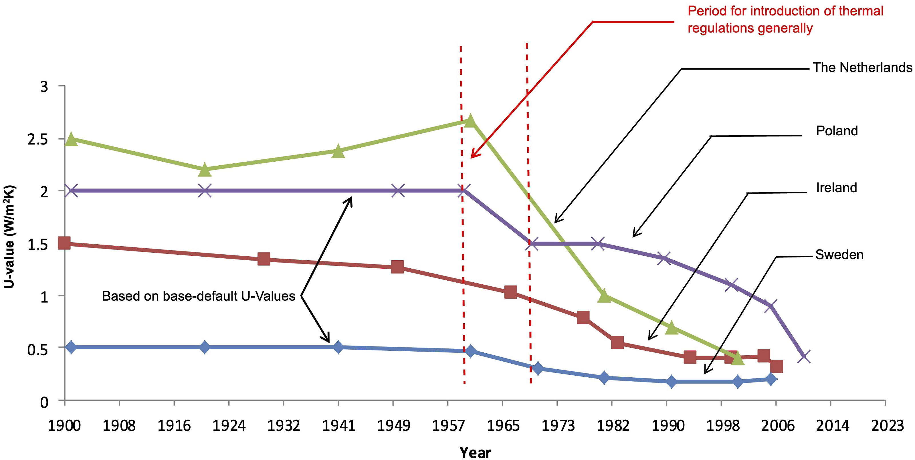

Figure 1.

Historical trends in U-values for external walls in four countries.^{35, 48}

The inconsistencies in reporting stock U-values raise concerns about their accuracy in representing actual thermal building stock conditions. For instance, the default U-Value for pre-thermal-regulations dwellings in Ireland is 2.1 W/m²K.⁹ However, the data in Figure 1 for Ireland is informed by Ireland’s national EPC database. If the pre-thermal regulation default U-value of 2.1 W/m²K were used (see Table 1) to indicate the relative thermal efficiency of the Irish building stock, Ireland’s stock would present as performing more poorly than that in Poland and Sweden but better than that in The Netherlands. As EPC empirical data for Ireland is used (default U-values stripped from the dataset as in 4), a truer (less-pessimistic) picture of the stock is presented. Indeed, Table 2 presents the relative change in U-Values of building elements over time in Ireland, showing how the average U-values change over time because of newer, more thermally efficiency stock being added to the stock as well as thermal retrofits over time.

Table 2.

Estimated empirical U-Values indicating the thermal performance of Irish housing^48,49.

		Walls		Roof		Double-glazed windows		Floor		Source
		%	Mean U-value (W/m²K)	%	Mean U-value (W/m²K)	%	Mean U-value (W/m²K)	%	Mean U-value (W/m²K)	Source
Year of survey	2001	56	1.01	82	1.3	61	-	25^¤	0.6	(49–51)
Year of survey	2014	58	0.66	67	0.37	97	2.92	53	0.59	(4)

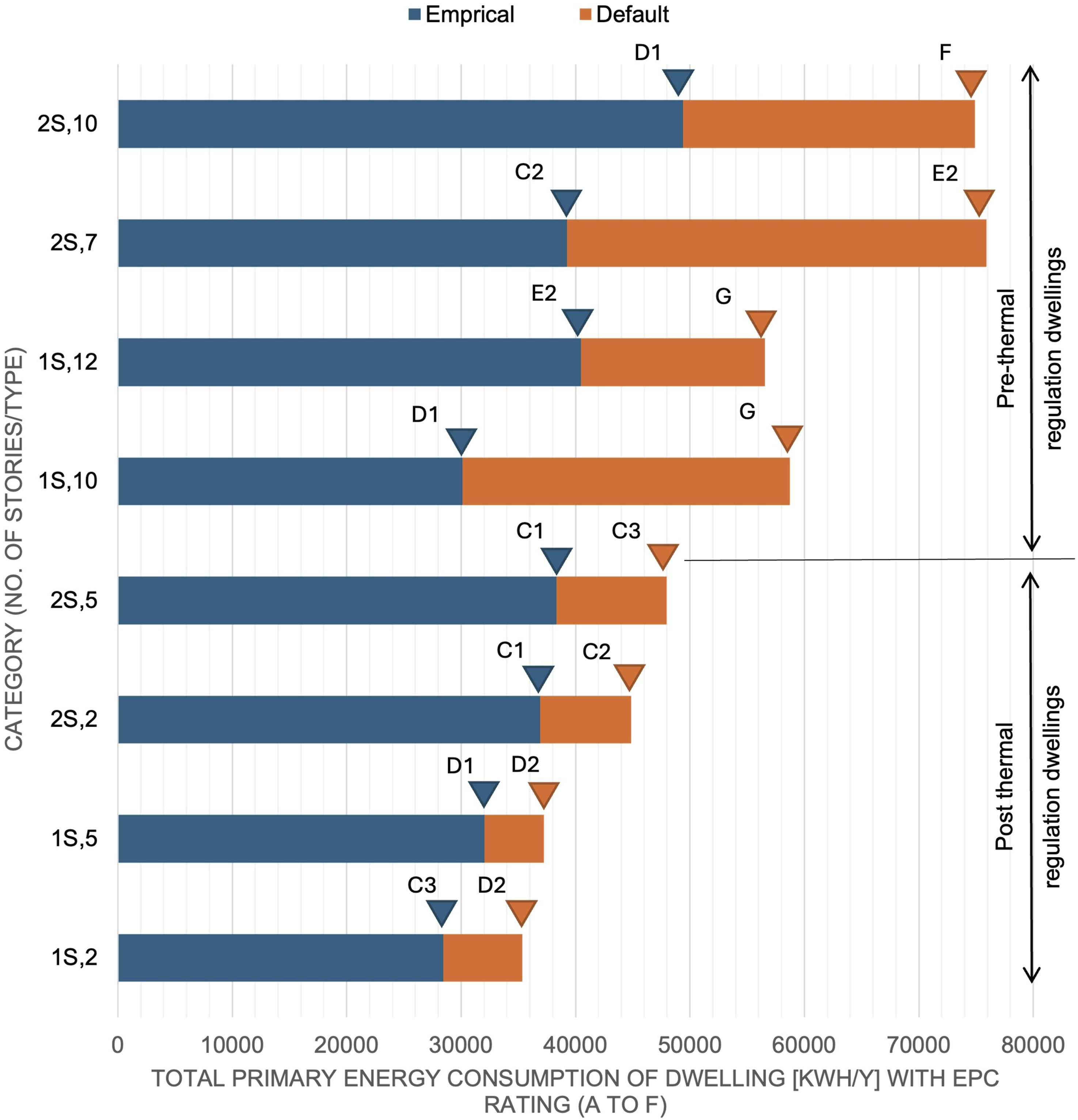
Over selection of defaults causes a systematic ‘default effect’ error in large national EPC datasets.⁵² Figure 2 illustrates ‘the default effect’ where in use of thermal default values results primary energy consumption associated with both primary and secondary heating systems increased by 31% for post-thermal regulation dwellings and 92% for pre-thermal regulation dwellings when default U-values are assumed over empirical values. For the dataset considered⁵³ thermal default use overestimate potential primary energy savings from upgrading by 22% and by 70% in dwellings built before after and before thermal building regulations respectively.

Figure 2.

Total primary energy consumption and associated energy rating for selected empirical and default reference dwellings as calculated by the DEAP methodology.⁵²

As the validity of U-Values used to indicate stock efficiency is therefore important,^54–56 they should be derived from empirical evidence, rather than assumed defaults.

As stated, default U-values are intended to be pessimistic. When selecting how pessimistic default U-values should be, the key issue, is the potential impact of that selection point on the EPCs accuracy. As shown in Figure 3, a 2016 in-depth study on default U-values examined the statistical relevance and effect of assuming pessimistic default U-values on dwelling energy performance certification quality in Ireland,⁴⁰ As shown in Figure 3, the study examined the implications of ‘moderately’ to ‘very pessimistic’ default values on certification quality, finding that a ‘reasonably’ pessimistic default U-value, derived from the 90th percentile point of the frequency distribution of U-Values, will ensure a reasonable level of accuracy for the certificate⁴⁰ but also allow the home-owner to perceive the energy advantage of carrying out thermal retrofits.⁴⁰ This study⁴⁰ also emphasised the need for continuous updates to default U-values based on EPC database insights, ensuring that these values remain reflective of evolving building stock conditions. This is because as the stock evolves towards higher levels of insulation, the mean of the distribution lowers accordingly, meaning, the default must be revised to remain reasonably pessimistic rather than become, ‘pessimistic’ to ‘very pessimistic’ or indeed ‘outmoded’ which is currently the case with Irish default U-values.

Figure 3.

Relationship of default U-value selection to quality aspects of energy performance certification relative to normal statistical distribution.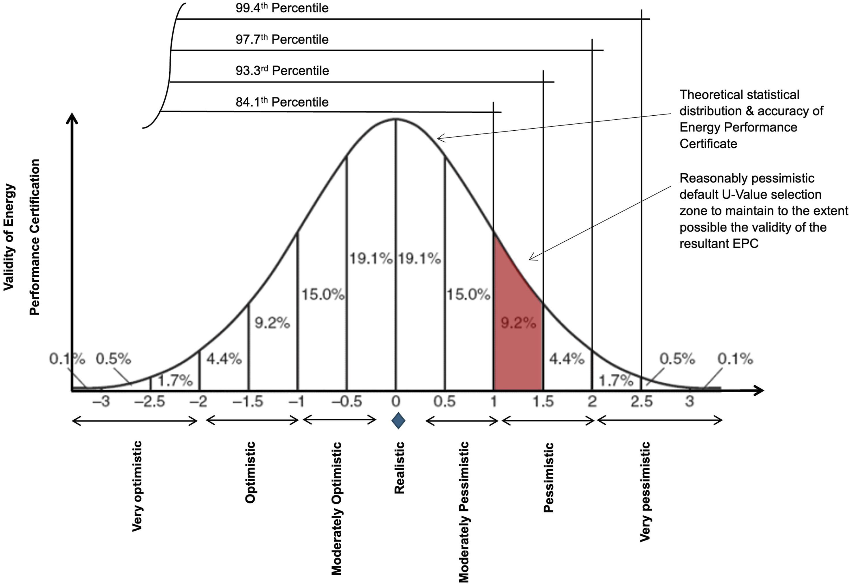

Likely distribution of an empirical EPC dataset

EPC U-value data was tested for correlation with the following distributions: Generalized Pareto, Inverse Gaussian, Logistic, Log-logistic, Lognormal, Nakagami, Normal, Rayleigh, Rician, t location-scale, Weibull, Birnbaum-Saunders, Exponential, Extreme value, Gamma, Generalized extreme value.

Figure 4 shows typical wall and roof U-value data in the EPC dataset wherein the U-value data is distributed with an asymmetric bimodal characteristic. Mode 1 represents well-insulated thermally upgraded dwelling element U-values whilst Mode 2 reflect more poorly insulated as-built dwelling elements. As shown in Figure 4, it is possible to ascertain the percentage of stock with thermally upgraded wall or roof elements and the percentage of stock that remains as-built (indicated by lower U-values). Figure 4 presents a typical distribution by a randomly selected construction period noting that the distribution holds through for all construction periods (pre and post thermal regulation) as evidenced in referance 4.

Figure 4.

Illustrative typical frequency distribution and analysis of wall and roof U-value by construction period.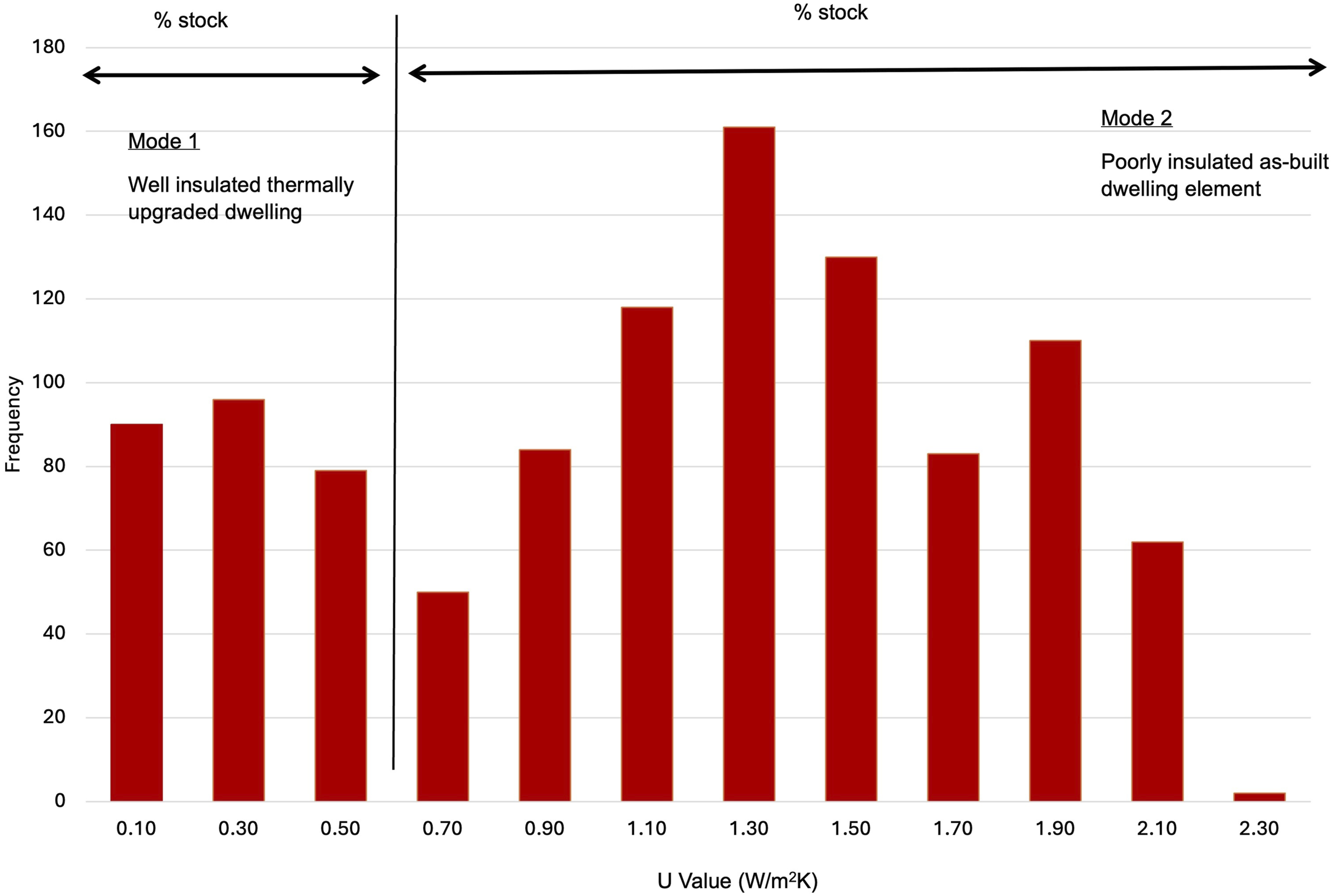

Understanding particular features of distributions is greatly enhanced if they correspond to specific parameters.² Referring to Figure 4:

• Mode 2 dwellings are as constructed originally with U-values for walls and roofs circa 0.6 to 2.3 W/m²K.

• Mode 1 dwellings are thermally upgraded, with U-value ranging between circa 0.1 to 0.59 W/m²K.

• As more thermal retrofits are carried-out, dwellings and their U-values migrate from the Mode 2 category to the Mode 1.

• Median U-values for Mode 1 dwellings are consistent within the range prescribed within the 2007⁵⁷ and 2011⁵⁸ Irish building regulations of 0.21 (2011) to 0.27 (2007) W/m²K for walls and 0.16 (2011) to 0.22 (2007) W/m²K for roofs.

• Energy refurbishment grants are available to homeowners⁵⁹ for walls that achieve a U-Value of 0.27 W/m²K and roofs that achieve a U-value of 0.16 W/m²K for ceiling-level insulation and 0.2 W/m²K for rafter insulation. Peaks in the Mode 1 dwellings distribution correspond to these U-values.

• Thermal retrofits harmonise levels of thermal insulation. Therefore, Mode 1 dwellings U-values have a lower standard deviation than those for Mode 2 dwellings.

Unlike walls and roofs, dwelling floors typically display a Normal unimodal distribution, assumed to result from fewer thermal retrofits of floors arising from; (i) the high cost of replacement floor coverings⁵¹ and (ii) the difficulties of retrofitting floor insulation.

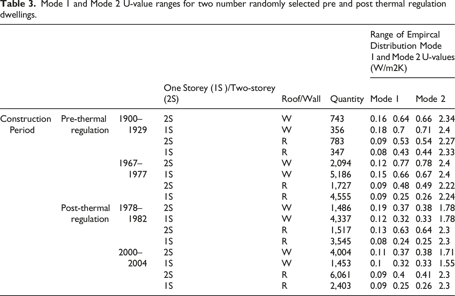
The empirical dataset was split into Mode 1 and Mode 2 data by dwelling element type, by construction period. Aside from construction period, there are two main periods of analysis; the period before the introduction of thermal requirements in building regulations and the period since thermal requirements have been included in building regulations. Thermal building regulations came into force in the mid-1970s leading to sharp rise in levels of thermal insulation in newly built buildings that had correspondingly lower U-values. Construction periods in Ireland are classified as⁹;

• Pre thermal regulation (5 construction periods: pre-1900, 1900 to 1929, 1930 to 1949, 1950 to 1966, 1967 to 1977); and

• Post thermal regulation (five construction periods: 1978 to 1982, 1983 to 1993, 1994 to 1999, 200 to 2004, 2005 to 2006 and post 2006).

To represent both thermal regulation periods, data for single and two-storey roof and wall characteristics was randomly sampled for two pre thermal regulations and two post-thermal regulations construction periods accounting for four of 10 construction periods or 40% of the EPC dataset. The following construction periods were selected:

• Pre thermal regulation (periods selected: 1900 to 1929, and 1967 to 1977); and

• Post thermal regulation (periods selected: 1978 to 1982 and 2000 to 2004).

As shown in Table 3, the selection set resulted in 16 U-value datasets comprised of 20,938 walls and 19,659 roofs. The U-value dataset by dwelling element and construction period was split into Mode 1 and Mode 2 (ref Figure 2) dwellings resulting in 32 datasets.

Table 3.

Mode 1 and Mode 2 U-value ranges for two number randomly selected pre and post thermal regulation dwellings.

						Range of Empircal Distribution Mode 1 and Mode 2 U-values (W/m2K)
			One Storey (1S )/Two-storey (2S)	Roof/Wall	Quantity	Mode 1		Mode 2
Construction Period	Pre-thermal regulation	1900–1929	2S	W	743	0.16	0.64	0.66	2.34
			1S	W	356	0.18	0.7	0.71	2.4
			2S	R	783	0.09	0.53	0.54	2.27
			1S	R	347	0.08	0.43	0.44	2.33
		1967–1977	2S	W	2,094	0.12	0.77	0.78	2.4
			1S	W	5,186	0.15	0.66	0.67	2.4
			2S	R	1,727	0.09	0.48	0.49	2.22
			1S	R	4,555	0.09	0.25	0.26	2.24
	Post-thermal regulation	1978–1982	2S	W	1,486	0.19	0.37	0.38	1.78
			1S	W	4,337	0.12	0.32	0.33	1.78
			2S	R	1,517	0.13	0.63	0.64	2.3
			1S	R	3,545	0.08	0.24	0.25	2.3
		2000–2004	2S	W	4,004	0.11	0.37	0.38	1.71
			1S	W	1,453	0.1	0.32	0.33	1.55
			2S	R	6,061	0.09	0.4	0.41	2.3
			1S	R	2,403	0.09	0.25	0.26	2.3

Maximum likelihood, Bayesian Information Criterion (BIC), Akaike Information Criterion (AIC), and an AIC with a correction factor for finite sample sizes were used to determine the best-fit distribution to the data. When fitting models, it is possible to increase the likelihood by adding parameters. However doing so may result in overfitting, that is the inclusion of more parameters than can be justified by the “noise” in the data leading to the distribution (i) failing to fit to additional data or (ii) unreliably predicting future observations. Both BIC and AIC attempt to resolve this by introducing a penalty term for the number of parameters in the model; the penalty term is larger in BIC than in AIC. As shown in Figure 2, all four parameters give very similar results in the cases tested.

It is evident from Figure 5 that no distribution is a perfect fit to the data. To determine if the best-fit distribution is a good fit to the empirical data, a chi-square goodness of fit test was carried out. With parameters estimated from the data, the chi-square goodness-of-fit tests the hypothesis that the data sample comes from a specified probability distribution. The chi-square test statistic is of the form shown in Equation.³

χ^{2} = \sum \frac{{(observed count - expected count)}^{2}}{expected count}

(3)

Figure 5.

Sample output from the “Find the Best Distribution” tool in MATLAB® (Sample shown, Mode 1, single story wall constructed between 1900 and 1929).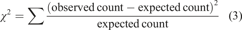

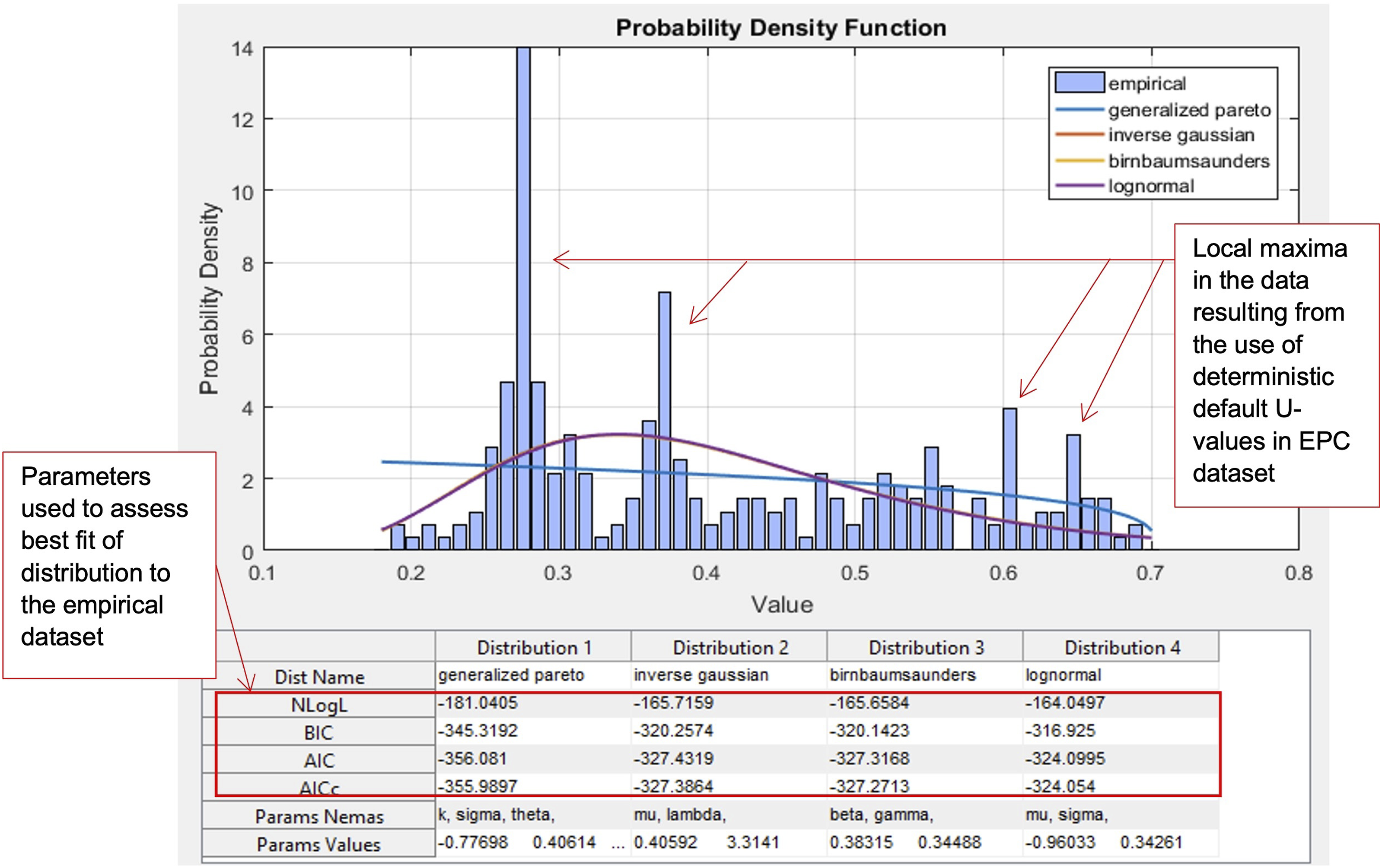
If the computed test statistic ( $χ^{2}$ ) is large, then the observed and expected values are not close and the model is a poor fit to the data. The hypothesis test result is returned as H₁ or H₀. The null hypothesis (H₀) suggests that the measured data are random values generated from the fitted distribution (i.e. that the distribution is a “good fit”). The alternative hypothesis (H₁) is that the distribution is not a good fit. The probability ( $p$ value) of obtaining the measured values if the null hypothesis is true was calculated for the distributions listed in Figure 5. Tests at 5% level of significance is the accepted norm for a chi-square test.⁶⁰ If the returned $p$ value ≥0.05 (5%), there is no evidence to reject the null hypothesis. If the returned $p$ value <0.05 (5%) there is evidence to reject the null hypothesis, or in other words, there is evidence that the data does not come from the distribution tested.

Except for a two-storey wall constructed between 2000 and 2004, the data did not fit any distribution in the 32 datasets tested. In the case of data set for a two-storey wall constructed between 2000 and 2004, it was determined that the log-logistic distribution fitted the data to a 1% significance level, and even this was a poor fit.

The finding that no standard statistical distribution fits the data arises from the empirical data is a mixture of actual U-values and default U-values. The over-selection of deterministic default U-values by the assessor,⁵² in favour of observed or measured U-values, leads to local peaks and noise in the data; as highlighted in Figure 5. Default U-values disrupt normal uncertainty factors, so no distribution presents a good fit to the data.

To establish a likely distribution of ‘measured’ U-values if deterministic default U-values were not present, a typical composite wall was simulated.

Likely distribution of simulated actual U-values

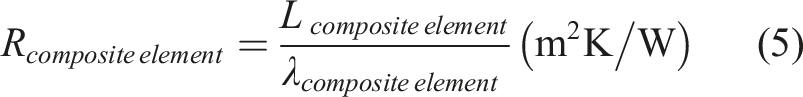
To establish a likely distribution of U-values arising from uncertainty factors inherent in measured values a common vernacular wall type¹¹ was selected for analysis. Solid limestone wall construction was common in Ireland up until the 1930s. This 300 mm to 500 mm thick wall is usually rendered externally and plastered internally with a 13 mm lime plaster. For a composite structure, as given by Equation,¹ the U-value is given by the reciprocal of the sum of the thermal resistances of the composite layers. The sum of the thermal resistance coefficient ‘R’ (∑R) of a composite structure is,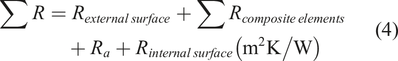

\sum R = {R_{e x t e r n a l s u r f a c e} + \sum R}_{c o m p o s i t e e l e m e n t s} + R_{a} + R_{i n t e r n a l s u r f a c e} (m^{2} K / W)

(4)

where

R_{c o m p o s i t e e l e m e n t} = \frac{L_{c o m p o s i t e e l e m e n t}}{λ_{c o m p o s i t e e l e m e n t}} (m^{2} K / W)

(5)

Values used for thermal conductivities of materials vary with assumed density and information source. Thermal conductivities for common construction materials in Ireland are sourced from the Irish Building Regulations,⁶¹ IS EN 12524, 2000, Building materials and products – hygrothermal properties – tabulated design values¹,⁶² and Chartered Institute of Building Services Engineers (CIBSE) Guide A.⁶³

Based on the depth of the wall and the presence of render or plaster in conjunction with the assumed thermal conductivities of the composite materials listed in CIBSE Guide A,⁶³ the U-value of a traditional limestone wall can be expected to range widely from 1.8 W/m²K to 3.6 W/m²K. As shown in Equation,⁵ the range is determined primarily by the depth (L in metres) of the wall, render and plaster (where present) and range of likely thermal conductivities possible (as given by CIBSE Guide A);⁶³

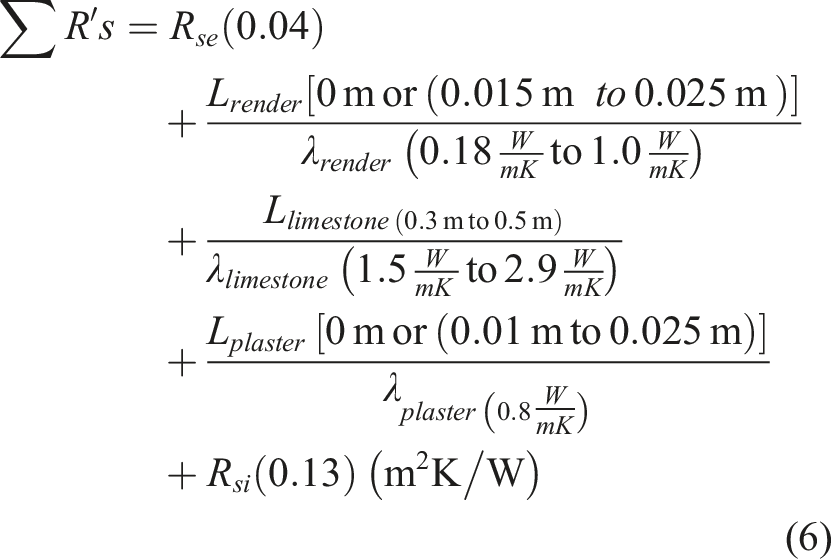
\sum R^{'} s = R_{s e} (0.04) + \frac{L_{r e n d e r} [0 m or (0.015 m t o 0.025 m)]}{λ_{r e n d e r} (0.18 \frac{W}{m K} to 1.0 \frac{W}{m K})} + \frac{L_{l i m e s t o n e (0.3 m to 0.5 m)}}{λ_{l i m e s t o n e} (1.5 \frac{W}{m K} to 2.9 \frac{W}{m K})} + \frac{L_{p l a s t e r} [0 m or (0.01 m to 0.025 m)]}{λ_{p l a s t e r (0.8 \frac{W}{m K})}} + R_{s i} (0.13) (m^{2} K / W)

(6)

Within the ranges shown in Equation,⁶ the ‘RAND’ function in Excel® was used to generate random values for the thermal conductivities of the render and limestone and the depth of render and plaster. The following are the parameters for the RAND function;

• External Render: Varied from 15 mm to 25 mm in depth, while conductivity varied between 0.18 W/mK and 1 W/mK

• Limestone: Varied from 300 mm to 500 mm in depth, while conductivity varied between 1.5 W/mK and 2.9 W/mK.

• Internal Plaster: Varied from 10 mm to 35 mm in depth, with a conductivity of 0.8 W/mK

The limestone wall was stepped in 50 mm variations all other values were randomised. Application of these parameters generated 10,000 U-values for a traditional limestone wall; the minimum U-value resulting was 1.67 W/m2K and the maximum U-Values was 3.67 W/m²K with a mean of 2.67 W/m²K and a standard deviation of 0.32 W/m²K.

It was assumed that outside render is present in 60% of walls with the remaining 40% having a stone finish while internal walls have a stone finish 20% of the time with lime plaster present 80% of the time. For those walls that were assumed rendered and/or plastered, a Normal distribution with six standard deviations (capturing 99.73% of the data +/− 3σ of the mean) was used to distribute depth of the render and plaster within the ranges shown in Equation.⁶ Wall depth was stepped in 50 mm stages from 300 mm to 500 mm; it was assumed that each depth occurred uniformly 20% of the time. In the simulation, random values of each of the three composite wall elements were used to generate 10,000 possible wall configurations.

A Gamma distribution was the best fit to the simulated data, however, the goodness of fit result was not significant, with a p-value of 0.0136 (1.36%). No distribution fitted the simulated U-value ‘measurement’ data to a 5% significance level.

Gori⁶⁴ created a method for the estimation of thermophysical properties of walls from short and seasonally independent in situ surveys that fitted a Lognormal distribution to thermal resistance values based on:

(i) An expectation of a Normal distribution arising from uncertainly factors associated with measured data (if deterministic values are not present);

(ii) The suggestion of the;

(a) Gamma distribution for the simulated U-value data along with

(b) lognormal distribution for in situ measurement of thermal resistance values by the literature.

Normal, Lognormal and Gamma distributions fitted to the simulated data are shown in Figure 6. The Lognormal and Gamma distribution functions achieve a slightly better fit to the simulated data, than the Normal distribution function, around the peak, but the Normal distribution fits the data better in the tails of the distribution.

Figure 6.

Normal, Lognormal and Gamma fits to simulated U-value data for a sample wall (Period selected, pre-1900 to 1930).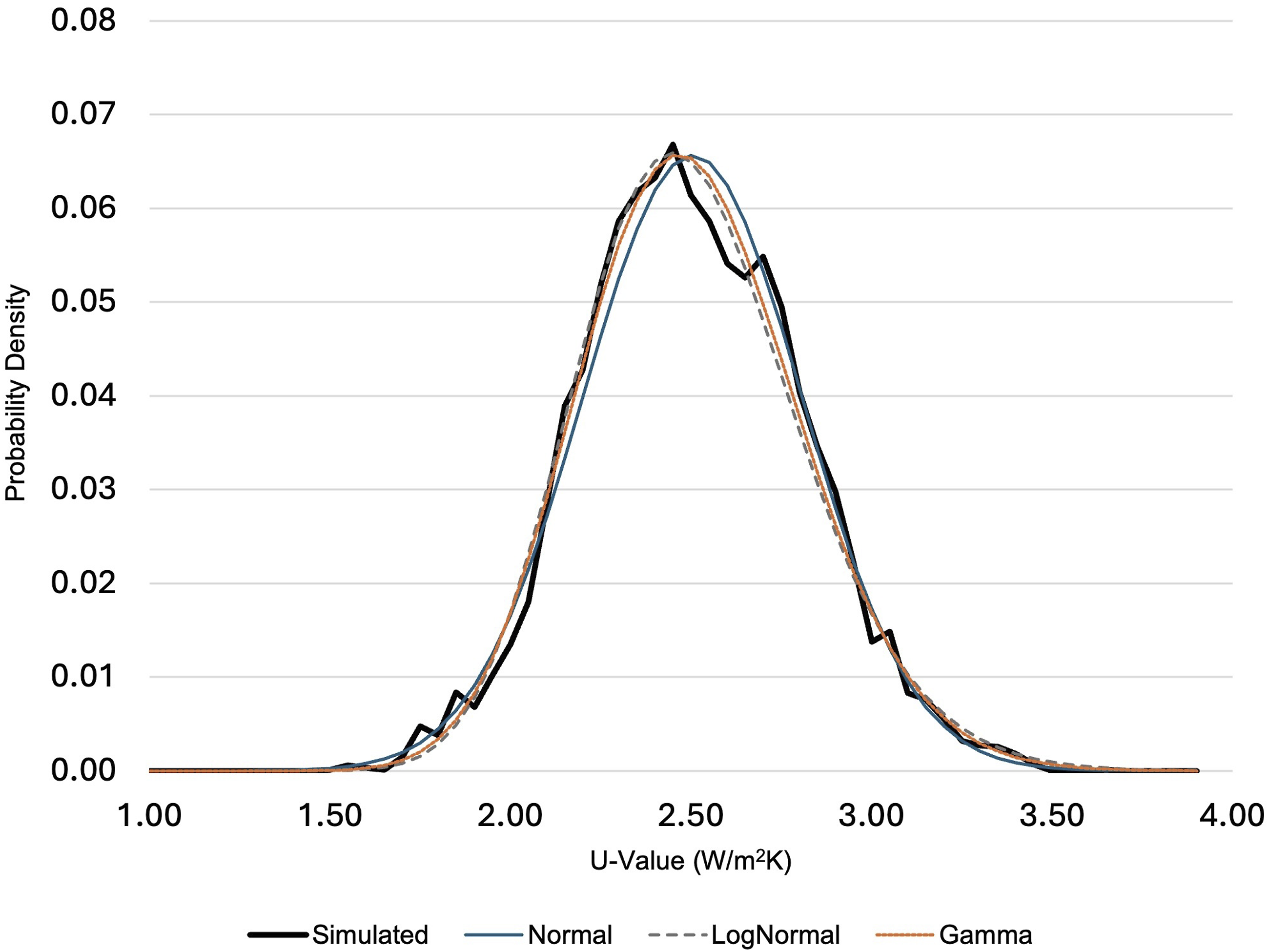

Figure 7 shows the Normal, Lognormal and Gamma datapoints presented as a percentage difference from the corresponding simulated data point. The Lognormal and Gamma distribution functions achieve a slightly better fit to simulated data around the peak while the normal distribution fits slightly better in the tails of the distribution. The variance in range above and below simulated data is as follows:

• Gamma; - 0.22% to +0.21% (Swing = 0.43%)

• Normal; - 0.32% to +0.27% (Swing = 0.59%)

• Lognormal; - 0.01% to +0.73% (Swing = 0.74%)

Figure 7.

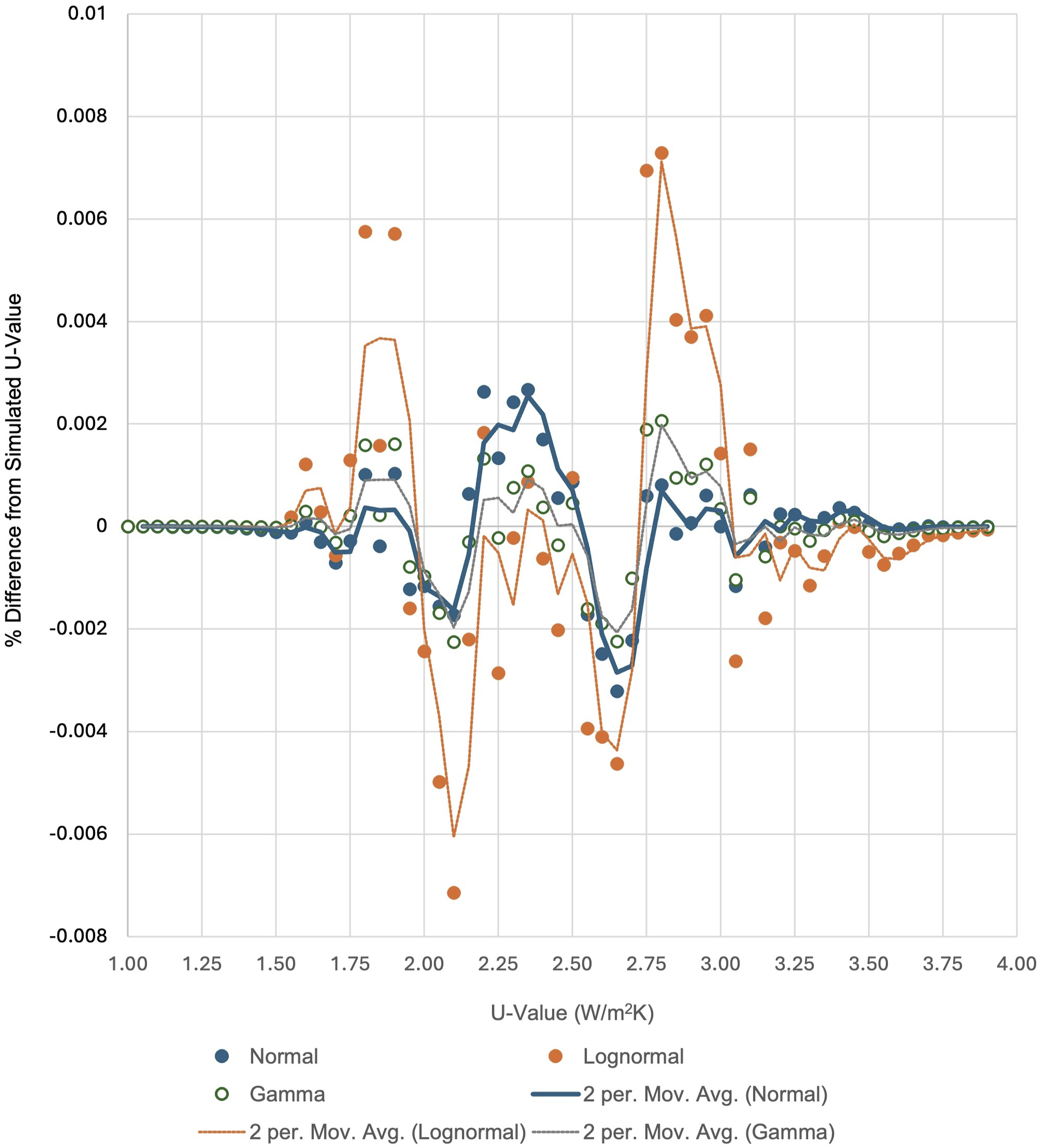
Percentage difference of Normal, Lognormal and Gamma fits to simulated U-value data for a sample wall (Period selected, pre-1900 to 1930).

As the percentage difference between the Gamma and Normal fit to simulated data, is less than 0.5% in all cases, no significant difference in fit was established.

Choices between distributions should be made primarily on the basis of important problem-specific requirements,⁶⁵ while straightforward mathematical formulae describing features of distributions enable insight, interpretation and clarity of exposition, as well as improving computational speed and convenience. In this context and to inform the selection of a suitable distribution to fit the empirical data, the impact of selecting different distributions on the results is assessed.

Selection of distribution function for the empirical data

Unlike with the Normal distribution the parameters of random variable (X), in this case U-values, transform when either the Lognormal or Gamma distribution is employed.

A Lognormal distribution is a continuous probability distribution of a random variable whose logarithm is normally distributed. The two parameters (µ) and (σ) are location and scale parameters for the natural logarithm $\ln (X)$ of the U-values; (µ) thus representing the mean of the natural logarithm of the U-values. The median of a Lognormal distribution is exp(µ), while its mean is exp (µ+σ²/2). The mean is larger than the median, indicating that the Lognormal distribution is right skewed.

The Gamma distribution is a two-parameter family of continuous probability distribution. When the random variable (X) is indexed by a function (I), the parameters of the Gamma distribution that best fit the empirical data are parameterised in terms of a shape parameter (α) and scale parameter (β) given by Equations⁷ and⁸;

α = \frac{M e a n {(X, I)}^{2}}{V a r i a n c e (X, I)}

(7)

β = \frac{V a r i a n c e (X, I)}{{M e a n (X, I)}^{2}}

(8)

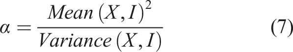
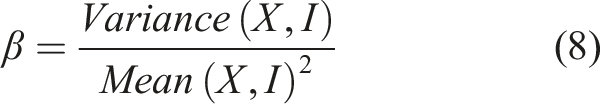
The Gamma distribution has a theoretical mean of (αβ) and theoretical variance of (αβ²) while the standard deviation of a Gamma distribution is given by $(β \sqrt{α})$ .

As the shape and scale parameters of the Lognormal and Gamma transform on distribution, it is not possible to compare the mean and modes of the Normal, Lognormal and Gamma probability distribution functions directly (formulae for the theoretical means and standard deviations of the Lognormal and Gamma are used to compare results with the Normal).

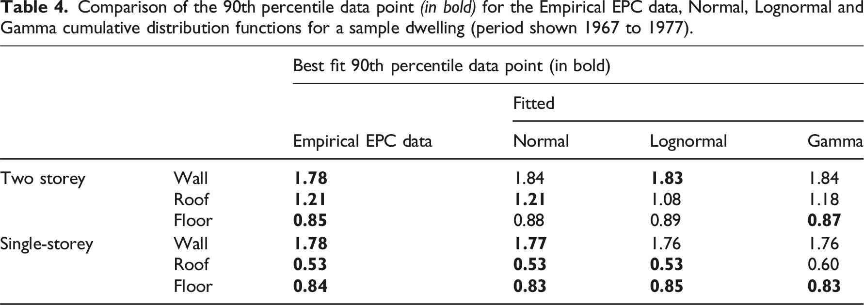
A direct comparison can be made easily between the individual and independent data points of the empirical and fitted cumulative distribution functions.

To determine statistically derived default U-values, previous research has studied the 90^th percentile point of empirical EPC U-value cumulative distribution functions by construction period. Table 4 compares the 90^th percentile point of cumulative distribution function arising from the fit of the Normal, Lognormal and Gamma distributions to a randomly selected construction period. Table 4 suggests that the Normal distribution presents a marginally better fit to the data than the other distribution tested, although the difference is not significant in terms of the sensitivity required of the results.

Table 4.

Comparison of the 90th percentile data point (in bold) for the Empirical EPC data, Normal, Lognormal and Gamma cumulative distribution functions for a sample dwelling (period shown 1967 to 1977).

		Best fit 90th percentile data point (in bold)
		Empirical EPC data	Fitted
		Empirical EPC data	Normal	Lognormal	Gamma
Two storey	Wall	1.78	1.84	1.83	1.84
	Roof	1.21	1.21	1.08	1.18
	Floor	0.85	0.88	0.89	0.87
Single-storey	Wall	1.78	1.77	1.76	1.76
	Roof	0.53	0.53	0.53	0.60
	Floor	0.84	0.83	0.85	0.83

Characterisation of a stock model from EPC data requires knowledge of the; (i) proportion of Mode 1 and Mode 2 and (ii) ‘Mean 1’ and ‘Mean 2’ of dwellings by construction period. The Normal distribution has the advantage of remaining Normal on transformation. Its mean, median and mode are the same and the entire distribution can be specified using just two parameters, mean and variance. The characteristics of the Normal distribution function simplifies the mathematics so enabling greater modelling convenience while also making the U-value distribution much easier to interpret and explain. Applying Occam’s Razor principle, in that the simpler solution is the best one given that all other things are same,⁶⁶ the Normal distribution is thus selected as a reasonable fit to the empircal data.

Validation and generalisability

The validity of selection of a Normal distribution to fit the empirical data is verified through evaluating the individual U-values with fitted data points estimated by the maximum likelihood method. A sample set of the individual data points for the 50^th, 75^th, 80^th, 85^th and 90^th percentile data points of the empirical and Normal fitted distribution by dwelling element and by construction period, resulting in 60 datasets, were matched and assessed for goodness of fit.⁴ Variance between the empirical and fitted data points that is greater than +/− 0.1 W/m²K was assessed. The fit of the Normal distribution to the data was found to be⁴;

• Good (maximum of one instance where variance greater than +/− 0.1 W/m^2K) in 82% of cases.

• Reasonable (two instances where variances greater than +/− 0.1 W/m²K) in 8.3% of cases.

• Sub-optimal (three instances where variances greater than +/− 0.1 W/m²K) in 9.7% of cases.

The analysis demonstrates:

• A reasonable to good fit in the vast majority (90.3%) of cases;

• The data points of the Normal fitted distribution to be equally likely to be below or above the empirical data points i.e. are Normal.

Internal validation is used where it is not possible to obtain a new independent external sample from the same population or a similar one. One method for good internal validation of a model’s performance is repeated data-splitting.⁶⁷ The EPC dataset was split in many ways; detached dwellings were isolated from the larger dataset, rural detached dwellings were isolated, dwellings were hence classified by number of stories, then by 10 construction periods followed by dwelling element (wall, roof, floor etc.). A Normal distribution was fitted repeatedly to each split dataset. The robustness of the method is demonstrated by consistent goodness-of-fit of the cumulative distribution function to the real data as shown in 4.

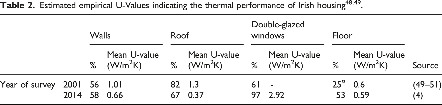
To externally validate the methodology, an independent sample from the same population was isolated from the original EPC dataset.⁴⁸ The methodology is validated externally as the appropriateness of the method is defended by the goodness-of-fit of the fitted to the real curve for a different housing typology.

Limitations and recommendations for further research

One of the fundamental limitations in interpreting U-value datasets lies in the inherent uncertainty of U-value assessment itself. Calculated U-values typically rely on idealised material properties, assumed layer configurations, and standardised thermal conductivity values, which may not accurately reflect the actual construction - especially in older or retrofitted buildings. Similarly, modelled U-values often apply default parameters and simplified moisture assumptions that do not adequately capture the dynamic hygrothermal behaviour of real materials. Empirical evidence, such as that reported in Reference 68, shows that these assumptions can lead to significant overestimation of U-values - up to 40% in traditional Irish brickwork - particularly where standard thermal conductivity values do not account for local material properties or in situ moisture conditions. Measured U-values, while more representative of actual performance, are themselves influenced by external variables such as ambient conditions, workmanship variability, and construction defects, as discussed in Reference 69. These compounded uncertainties suggest that caution must be exercised when interpreting distributions of U-values, as discrepancies between assumed, modelled, and measured values may distort conclusions about performance norms and retrofit effectiveness.

The presence of default U-values in EPC datasets introduced artificial distortions, making statistical modelling more complex. Future studies should explore methods to filter or adjust for these artefacts. The findings are based on Irish EPC data, and while the methodology is generalisable, further validation is required for other European building stock datasets. While Lognormal and Gamma distributions provided slightly better peak fits, the Normal distribution was chosen for its mathematical convenience. Alternative multi-modal approaches or machine learning-based clustering could improve future analyses.

While this study does not propose revised default U-values, the findings highlight substantial divergence between empirical U-value distributions and commonly applied regulatory defaults. This misalignment suggests that default values currently used in EPC and compliance assessments may not adequately reflect actual building stock performance, particularly for pre-1980 constructions. As such, our results reinforce the need for recalibrating default U-values based on statistically representative datasets. The work by Raushan et al. (2022)¹¹ provides a methodological pathway for substituting more realistic values into EPC databases, and further research should build on such approaches to ensure regulatory assumptions are evidence-based and context-specific.

Developing data-driven dynamic U-value defaults that update as the building stock evolves could significantly enhance energy modelling accuracy. Advanced techniques such as Bayesian inference, Gaussian Mixture Models (GMMs), or deep learning algorithms may to identify hidden patterns in U-value distributions. It should be explored if integration of more-refined U-value distributions with policy models: alters cost-optimal refurbishment objectives under the EPBD. Extending this methodology to other European EPC datasets may provide comparative analyses of national U-value variations may offer insights into how policies and strategies affect building stock thermal energy efficiency.

Conclusions

The presence of default U-values in Energy Performance Certificate (EPC) databases significantly disrupts the natural variability in measured U-value distributions. Default U-values, often used by assessors when empirical data is unavailable, introduce deterministic values into datasets, creating artificial peaks that misrepresent the true distribution of U-values. As a result, standard statistical distributions fail to model EPC U-value data accurately. This issue affects the reliability of national building stock models, potentially leading to misinterpretations of energy performance and policy inefficiencies.

To determine a best-fit distribution for measured U-values, multiple statistical functions were tested, including Normal, Lognormal, and Gamma distributions. Lognormal and Gamma distributions provided slightly better fits around the peak of the dataset, while the Normal distribution was more accurate in the tail regions. The Normal distribution has the advantage of remaining Normal on transformation. This means its mean, median and mode remain the same. As the entire distribution can be specified using just its mean and variance, the U-value distribution is easier to analyse, interpret and explain. Applying Occam’s Razor principle, that the simpler solution is the best one given that all other things are same, the Normal distribution is selected as a reasonable fit to empircal U-values within the EPC dataset. The selection was validated internally through data splitting, externally through use of a new independent sample, and with the use of simulated data.

The findings show that over-reliance on outdated default values distorts national energy models and affects the accuracy of bottom-up stock modelling approaches used in policy development. Introducing data-driven dynamic default U-values, which evolve as building stock characteristics change, could significantly improve the accuracy of energy efficiency assessments at the national scale.

A bimodal distribution within the EPC dataset reflects the presence of two distinct dwelling categories:

• Mode 1: Thermally upgraded dwellings with lower U-values.

• Mode 2: Older dwellings with higher U-values that have yet to undergo significant retrofits.

As energy efficiency policies drive retrofit programs, the distribution of U-values will change as more dwellings fall within Mode 1 than Mode 2. This shift will require continuous reassessment of U-value benchmarks to maintain model accuracy.

In summary, this study demonstrates that,

• No single standard statistical distribution fits EPC U-value data due to the presence of deterministic default U-values

• For measured U-values, Normal, Lognormal, and Gamma distributions provided best fits,

• A Normal distribution offers the most practical and interpretable solution,

• The selected Normal distribution allows for more transparent and computationally efficient modelling, improving the accuracy of national bottom-up energy models,

• Default U-values must be updated based on empirical trends to ensure they reflect the evolving building stock.

Footnotes

Declaration of conflicting interests

The author(s) declared no potential conflicts of interest with respect to the research, authorship, and/or publication of this article.

Funding

The author(s) disclosed receipt of the following financial support for the research, authorship, and/or publication of this article: This work was supported by the This research was supported by MaREI, the SFI Research Centre for Energy, Climate and Marine [Grant No: 12/RC/2303-P2] and SEAI RD&D Grant No. 22/RDD/855 and 23/RDD/1046.

ORCID iD

C. Ahern

Data Availability Statement

The data that support the findings of this study are openly available from; Ahern, Ciara (2019), “Ireland predominant housing typology dataset ”, Mendeley Data, V1, .⁵³

Note

Appendix

References

Kavgic

Mavrogianni

Mumovic

, et al. A review of bottom-up building stock models for energy consumption in the residential sector. Build Environ 2010; 45(7): 1683–1697.

Jones

. On families of distributions with shape parameters. Int Statistical Rev 2015; 83(2): 175–192.

SEAI . National BER research tool 2014. Available from: https://ndber.seai.ie/BERResearchTool/Register/Register.aspx

Ahern

. Introducing the default effect: reducing the gap between theoretical prediction and actual Energy consumed by dwellings through characterising data more representative of national dwelling stocks. Dublin, Ireland: Technological University Dublin, 2019.

SEAI . Dwelling energy assessment procedure (DEAP) survey Guide. Dublin, Ireland: The Sustainable Energy Authority of Ireland, 2012.

Rasooli

Itard

Ferreira

. A response factor-based method for the rapid in-situ determination of wall’s thermal resistance in existing buildings. Energy Build 2016; 119(Supplement C): 51–61.

van den Brom

Meijer

Visscher

. Performance gaps in energy consumption: household groups and building characteristics. Garston: Building Research & Information, 2017, pp. 1–17.

Lowe

. Addressing the challenges of climate change for the built environment. Build Res Inf 2007; 35(4): 343–350.

SEAI. Dwelling Energy Assessment Procedure (DEAP) . Irish official method for calculating and rating the energy performance of dwellings. Dublin, Ireland: SEAI, 2012.

10.

SEAI . What are the carbon emission factors used? 2017. Available from: https://www.seai.ie/Your_Business/Public_Sector/FAQ/Energy_Reporting_Overview/What_are_the_carbon_emission_factors_used.html

11.

Raushan

Ahern

Norton

. Determining realistic U-values to substitute default U-values in EPC database to make more representative; a case-study in Ireland. Energy Build 2022; 274: 112358.

12.

Commission E . Energy statistics - an overview, (n.d.). Brussels: European Commission; 2024 Available from: https://ec.europa.eu/eurostat/statistics-explained/index.php?title=Energy_statistics_-_an_overview

13.

Ahern

Norton

. A generalisable bottom-up methodology for deriving a residential stock model from large empirical databases. Energy Build 2020; 215: 109886.

14.

Huebner

Hamilton

Chalabi

, et al. Explaining domestic energy consumption – the comparative contribution of building factors, socio-demographics, behaviours and attitudes. Appl Energy 2015; 159: 589–600.

15.

Famuyibo

Duffy

Strachan

. Developing archetypes for domestic dwellings—an Irish case study. Energy Build 2012; 50(0): 150–157.

16.

van der Ham

Klein

Tabatabaei

, et al. Methods for a smart thermostat to estimate the characteristics of a house based on sensor data. Energy Proc 2016; 95(Supplement C): 467–474.

17.

Rodríguez-Soria

Domínguez-Hernández

Pérez-Bella

, et al. Review of international regulations governing the thermal insulation requirements of residential buildings and the harmonization of envelope energy loss. Renew Sustain Energy Rev 2014; 34: 78–90.

18.

van den Brom

Hansen

Gram-Hanssen

, et al. Variances in residential heating consumption – importance of building characteristics and occupants analysed by movers and stayers. Appl Energy 2019; 250: 713–728.

19.

Eurostat . Eurostat database. Luxembourg: European Union Luxembourg, 2019.

20.

Energy dashboard. 2021. [Accessed Spetember 2024], Available from:https://ec.europa.eu/eurostat/cache/infographs/energy_dashboard/endash.html?geo=EU27_2020&year=2019&language=EN&detail=1&nrg_bal=&unit=MTOE&chart=chart_1,chart_2,chart_3,chart_4,chart_5,chart_8&modal=0

21.

Stone

Shipworth

Biddulph

, et al. Key factors determining the energy rating of existing English houses. Build Res Inf 2014; 42(6): 725–738.

22.

Clinch

Healy

. Alleviating fuel poverty in Ireland, a program for the 21st century. International Journal of Housing Science 1999; 23(4): 203–215.

23.

Oreszczyn

Hong

Ridley

, et al. Determinants of winter indoor temperatures in low income households in England. Energy Build 2006; 38(3): 245–252.

24.

Firth

Lomas

. Investigation CO2 emission reductions in existing urban housing using a community domestic energy model. In: Eleventh international IBPSA conference; glasgow, scotland: department of civil and building engineering. UK: Loughborough University, 2009, pp. 2098–2105.

25.

Hamilton

Oreszczyn

Summerfield

, et al. Co-Benefits of energy and buildings data: the case for supporting data access to achieve a sustainable built environment. Procedia Eng 2015; 118: 958–968.

26.

Reeves

Taylor

Fleming

. Modelling the potential to achieve deep carbon emission cuts in existing UK social housing: the case of Peabody. Energy Policy 2010; 38(8): 4241–4251.

27.

Pasichnyi

Wallin

Levihn

, et al.

Energy performance certificates — new opportunities for data-enabled urban energy policy instruments?

Energy Policy 2019; 127: 486–499.

28.

Jenkins

Simpson

Peacock

. Investigating the consistency and quality of EPC ratings and assessments. Energy 2017; 138: 480–489.

29.

Beltrán-Velamazán

Monzón-Chavarrías

López-Mesa

. A new approach for national-scale Building Energy Models based on Energy Performance Certificates in European countries: the case of Spain. Heliyon 2024; 10(3): e25473.

30.

Pan

Debnath

, et al. Energy mapping of existing building stock in Cambridge using energy performance certificates and thermal infrared imagery. Environ Data Science 2024; 3(e44): e44.

31.

Aricpowska

Mariottini

. Role of the EU building stock observatory in evaluation of the buildings policies. In: 2016 International Energy Policies & Programmes Evaluation Conference, Amsterdam (The Netherlands), June 7 –9, 2021.

32.

Dong

Schwartz

Mavrogianni

, et al. A review of approaches and applications in building stock energy and indoor environment modelling. Build Serv Eng Res Tecnol 2023; 44(3): 333–354.

33.

Evans

Liddiard

Steadman

. Modelling a whole building stock: domestic, non-domestic and mixed use. Build Res Inf 2019; 47(2): 156–172.

34.

Tuominen

Holopainen

Eskola

, et al. Calculation method and tool for assessing energy consumption in the building stock. Build Environ 2014; 75: 153–160.

35.

Economidou

Atanasiu

Despret

, et al.

Europe’s buildings under the microscope - a country-by-country review of the energy performance of buildings 2011 Feb

2015. [Accessed Spetember 2023], Available from:https://www.institutebe.com/InstituteBE/media/Library/Resources/ExistingBuildingRetrofits/Europes-Buildings-Under-the-Microscope-BPIE.pdf

36.

EuroACE . Factsheet on cost-optimality. [Accessed August 2024]. Available from:https://www.euroace.org/LinkClick.aspx?fileticket=mB-AuwiKfcQ%3D&tabid=155

37.

Simpson

Banfill

Haines

, et al. Energy-led domestic retrofit: impact of the intervention sequence. Build Res Inf 2016; 44(1): 97–115.

38.

Ballarini

Corgnati

Corrado

. Use of reference buildings to assess the energy saving potentials of the residential building stock: the experience of TABULA project. Energy Policy 2014; 68(0): 273–284.

39.

Corgnati

Fabrizio

Filippi

, et al. Reference buildings for cost optimal analysis: method of definition and application. Appl Energy 2013; 102: 983–993.

40.

Ahern

Norton

Enright

. The statistical relevance and effect of assuming pessimistic default overall thermal transmittance coefficients on dwelling energy performance certification quality in Ireland. Energy Build 2016; 127: 268–278.

41.

EU . Commission Delegated Regulation (EU) No. 244/2012 of 16 January 2012 Supplementing Directive 2010/31/EU of the European Parliment and of the council on the energy perofrmance of buildings by establishing a compartive methodology framework for calculating cost-optimal levels of minimum energy performance requirement for buildings and building elements. Off J Eur Union 2012; 224: 244–2012.

42.

Ferrari

Zagarella

Caputo

, et al. Results of a literature review on methods for estimating buildings energy demand at district level. Energy 2019; 175: 1130–1137.

43.

Pérez-Lombard

Ortiz

González

, et al. A review of benchmarking, rating and labelling concepts within the framework of building energy certification schemes. Energy Build 2009; 41(3): 272–278.

44.

Badurek

Hanratty

Sheldrick

, et al. Building Typology Brochure Ireland - a detailed study on the energy performance of typical Irish dwelligns. Dublin: Elsevier, 2012.

45.

Sayfikar

Jenkins

. Energy performance certificate calculation methodologies across Europe and accommodating new performance indicators. Build Serv Eng Res Technol 2024; 46(1): 45–59.

46.

Arkesteijn

van Dijk

. Energy performance certification for new and existing buildings - differences in approach, the role of choice in CEN standards application. 2010. Available from: https://www.buildup.eu/sites/default/files/content/P156_EN_CENSE_New_and_existing_buildings.pdf. (Accessed January 2025).

47.

Papadopoulos

. Forty years of regulations on the thermal performance of the building envelope in Europe: achievements, perspectives and challenges. Energy Build 2016; 127: 942–952.

48.

Ahern

. National BER research tool. In: SEAI. Dublin, Ireland: SEAI; 2014.

49.

INSHQ . Irish national housing survey of Ireland. In: Institute EaSR. pp. 2001-2002.

50.

Ahern

Griffiths

O’Flaherty

. State of the Irish Housing stock - modelling the heat losses of Ireland's existing detached rural housing stock & estimating the benefit of thermal retrofit measures on this stock. Energy Policy 2013; 55: 139–151.

51.

P Clinch Jdh

. Quantifying the severity of fuel poverty, its relationship with poor housing and reasons for non-investment in energy-saving measures in Ireland. Energy Policy 2004; 32: 207–220.

52.

Ahern

Norton

. Energy Performance Certification: misassessment due to assuming default heat losses. Energy Build 2020; 224: 110229.

53.

Ahern

. Ireland's predominant housing typology dataset. In: SEAI. Dublin, Ireland: SEAI; 2014.

54.

FGN

Smith

AZP

Biddulph

, et al. Solid-wall U -values: heat flux measurements compared with standard assumptions. Build Res Inf 2015; 43(2): 238–252.

55.

Tamimi

Hassan

Rodriguez-Ubinas

, et al. Thermal performance of 3D concrete printed walls: calculated and in-situ measured U-values. J Asian Architect Build Eng 2024; 23(6): 1903–1915.

56.

Sang-Tae

Jeong

J-W

. Field measurement of U-value using multiple sensors at test chamber and EIFS building. J Asian Architect Build Eng 2019; 18(2): 60–68.

57.

Department of Environment HaLG. Building Regulations 2007 - Technical Guidance Document L . Conservation of fuel and energy - dwellings. Dublin, Ireland: The Stationery Office, 2007.

58.

DEC&LG . Technical guideance document L - conservation of fuel and energy - dwellings. Dublin, Ireland: Department of Environment, Community and Local Government, 2011.

59.

SEAI . A homeowner's Guide to wall Insulation2018 february 2018. Available from: https://www.seai.ie/resources/publications/Homeowners-Guide-To-Wall-Insulation.pdf

60.

Hoel

(ed). Introduction to mathematical statistics. 5th ed. canada. Hoboken: Wiley & Sons, Inc., 1984.

61.

Government of Ireland . Department of heritage and local government, conservation of fuel and energy - buildings other than dwellings. In: Building regulations - technical guidance document L. Dublin, Ireland: The Stationery Office, 2008.

62.

NSAI . IS EN 12524:2000 Building materials and products - hygrothermal properties - tabulated design values (No longer current but cited in Building Regulations guidance). Dublin, Ireland: National Standards Authority of Ireland, 2000.

63.

CIBSE . CIBSE Guide A; environmental design. London: CIBSE, 2006.

64.

Gori

. A novel method for the estimation of thermophyscial properties of walls from short and seasonally independent in-situ surveys. London, UK: University College London, 2017.

65.

Jones

. On families of distributions with shape parameters2018 November 2018. Available from: https://statistics.open.ac.uk/802576CB00593013/(httpInfoFiles)/FE2EE03EDE61AB8E80257C700040D68E/$file/review.pdf, (Accessed January 2025).

66.

Parbhakar

. Why data scientists love Guassian. Data Sci 2018, [Accessed May 2025], Available from:https://medium.com/data-science/why-data-scientists-love-gaussian-6e7a7b726859

67.

Harrell

Lee

Mark

. Multivariable prognostic models: issues in developing models, evaluating assumptions and adequacy, and measuring and reducing errors. Stat Med 1996; 15(4): 361–387.

68.

Hofheinz

Walker

Engel Purcell

, et al. Thermal conductivity testing of a range of Irish traditional bricks using Transient Line Source methodology. In: The seventh international conference on conservation of architectural heritage. Sustainability (CAH) University of Portsmouth, United Kingdom, 2023. Available from: https://researchrepository.ucd.ie/entities/publication/3f420f68-3737-4f45-90b8-68adfba2f766

69.

Papadakos

Marinakis

Konstas

, et al. Managing the uncertainty of the U-value measurement using an auxiliary set along with a thermal camera. Energy Build 2021; 242: 110984.

A method for determining a true national statistical distribution of building element U-values and its application to a dataset underpinning a building stock energy model

Abstract

Keywords

Highlights

Introduction

Background

Default U-values and their limitations

Likely distribution of an empirical EPC dataset

Likely distribution of simulated actual U-values

Selection of distribution function for the empirical data

Validation and generalisability

Limitations and recommendations for further research

Conclusions

Footnotes

Declaration of conflicting interests

Funding

ORCID iD

Data Availability Statement

Note

Appendix

References