Accurate representations of locally meaningful future extreme weather events and the implications for India

Abstract

It is now evident that periods of extreme temperature and humidity can transform buildings from places of shelter to sources of significant morbidity and mortality. Mitigating this risk requires computer representations of such events. Unfortunately, neither an agreed globally consistent representational method nor long-term continuous hourly weather data at a sufficient spatial resolution exist, from which such events can be extracted. Here, we introduce a new, mathematically sound, physically meaningful and consistent method to represent hot-dry, hot-wet and cold-dry extreme weather events of arbitrary length localised to the weather of the location in question, unlike existing methods that use absolute temperature thresholds regardless of locale. Importantly for human survival, this new method includes humidity. Replicable globally, we apply this method to India using carefully calibrated computer-generated weather data localised to 25 km (4790 locations) for now and the future, making India the first Global South country to obtain such an extreme event dataset. A series of tests show high consistency and reliability including low mean bias error against all known long-term (∼100 year) dry-bulb hot extremes of +0.2°C (σ = 2.4°C) and a mean deviation of 4.5°C (σ = 4.9°C) compared to the equivalent extreme period in a typical year. By moving a validated computer model of a typical apartment across all 4790 locations, we find significant, spatially varied, differences in indoor mean-maximum temperature and discomfort degree hours for a range of events, past (1981-2010) and future (2060-2089). Periods where mortality is likely to be significant are found. The reliability of the data, combined with their unprecedented spatiotemporal resolution and timescale, transforms our ability to study a wide range of weather-influenced phenomena, such as indoor and outdoor risks to human health or crop yields, under current and climate-changed weather.

Practical Application

There is an urgent need for the public and professionals to fully understand that the impacts of climate change will be most transformative with respect to extreme, not mean, temperatures; with mass mortality becoming common. The method introduced here for the creation of extreme timeseries is general and replicable globally. The files produced for the case of India are freely available and already in use via a public repository. They are helpful to building designers, urban planners, policymakers and professionals in a variety of fields to analyse performance under extreme conditions and the implications for human health.

Introduction

The public discourse around climate change often focuses on a mean increase in global surface temperatures. This obscures the fact that a gradual increase in a given location’s temperature will be accompanied by an increase in the severity, frequency, and duration of extreme temperature events. Indeed, several recent record-breaking extreme events^1,2 have been either in part or wholly attributed to the current modest mean warming of 1.1°C. ³ We can hence expect a future mean warming between 1.5 and 3°C to be accompanied by extremes of significant impact.

However, it is not merely temperature that is the issue, as humidity plays a significant role, especially in the ability of humans to effectively respond to a sudden perturbation in the weather. This is due to the fact that 90% of heat loss at air temperatures above 35°C occurs through evaporation of sweat, ⁴ which is impaired at high levels of humidity. In addition, although mean temperatures are increasing, one can continue to expect cold spells, which will also change in character in the future compared to the present. It is hence essential to study and plan for events involving varying combinations of high and low temperatures and humidity, as these can affect a range of systems, including buildings, agriculture, livestock, fisheries, transport and energy networks.

In buildings, these events can cause damage to building envelopes and mechanical systems but more commonly lead to increased energy demand for cooling or heating, resulting in disruptions to building operation when the demand cannot be met. These can cascade outwards into power grids, causing widespread failure and secondary impacts on industrial output and productivity. Such events can also directly impact the health and safety of building occupants, particularly vulnerable populations such as the elderly and those with pre-existing health conditions. ⁵ High temperatures are implicated in various health issues, such as dizziness, fatigue, and heat stroke, which can cause organ damage and even death. In addition, high temperatures accompanied by air pollutants (PM₁₀ / PM_2.5) show a rise in non-accidental and cardiovascular mortality. ⁶

It is therefore clear that it would be advantageous to have well-defined representations of weather extremes, ideally in machine-readable form. A dataset of such extremes could then be used to seed mathematical models or computer simulations to study and plan for the change in weather-related impacts on a range of human and natural systems between now and the future.

Unfortunately, there seems to be little agreement on the precise formulation of extreme weather events. Countries worldwide have adopted divergent definitions, especially around heat waves, often based on historic representational norms or expectations, as later discussed in Section 1.1.

This is just one dimension of the problem. The analysis and prediction of building performance using computer simulations uses hourly weather data for a year, that is 8760 rows of ‘synoptic’ weather data. Earlier work stipulates specific characteristics that an extreme weather file must possess.^7,8 Firstly, it must match the temporal resolution required by simulation packages, usually hourly, as earlier. Secondly, it should consider changes in weather patterns induced by local topography in the area of interest by having an adequate spatial resolution, for example between 5 and 25 km in the UK. ⁹ Thirdly, it ought to reflect the impact of local urban micro-climates. Fourthly, it should be able to generate extreme weather files for future periods while considering the effects of climate change. Finally, it must include at least one warm spell and exhibit a ‘temperature tail' that exceeds the corresponding TRY high temperatures.^7,8

It is clear from the above that, by definition, extracting such infrequent events will require a long time series of weather data. Unfortunately, in many parts of the world, hourly series at good spatial resolution do not exist even for the 30 years needed for generating typical weather files, much less for generating extreme weather files, which would require more prolonged periods. India, for example, has only 59 locations with continuous hourly data, that is one per 55,712 km² or, if evenly spaced, a grid size of 236 km. Even here, the number of years where data are of acceptable quality, that is the number of years where the source record contains more than 50% of data, averages just 11 years. ¹⁰ These include virtually no solar data, which are needed for accurate representations of heat gains in simulators such as EnergyPlus. Thus, it would be impossible to create representations of extreme weather using such basis data and require significant processing and imputation before representations of even typical weather can be extracted.

Hence, the only means of generating representations of extreme weather, mutually consistent between historic and future climate, would be using calibrated synthetic weather data where long time series can be generated. ⁷ This approach has been successfully used, for example in the UK using a weather generator trained on multi-model ensembles to produce weather files at 5 km resolution. ¹¹

We present two key innovations in this work. The first being a mathematically sound definition of extreme weather events that is both locally consistent and globally applicable. Secondly, a procedure to select dry and wet-bulb temperature extremes using a week as a convenient event time-frame, ¹² and to use this to generate representations of three key types of extreme events, that is “hot and dry”, “cold and dry” and “hot and humid”, using a long time series of weather data for 4790 locations obtained from the UK Met Office’s PRECIS dataset for India covering the period 1970 – 2100 at a 25 km spatial resolution. Finally, we illustrate the impact of these events on indoor temperatures by moving a validated thermal model across all locations.

Extreme events definitions

There is no single agreed definition for extreme events, with different countries adopting different norms based on localised tradition and the driving disciplines such as climate science, medicine or civil protection. ¹³ For example, the World Meteorological Organisation (WMO) does not offer an official definition for a heatwave but adopted the following definition to aid countries in defining and characterising extreme weather events: “A heatwave can be defined as a period of marked and unusually hot weather persisting for at least two consecutive days”. ¹⁴ Table 1 illustrates the disparity in definitions adopted by a selection of bodies and countries.

Table 1.

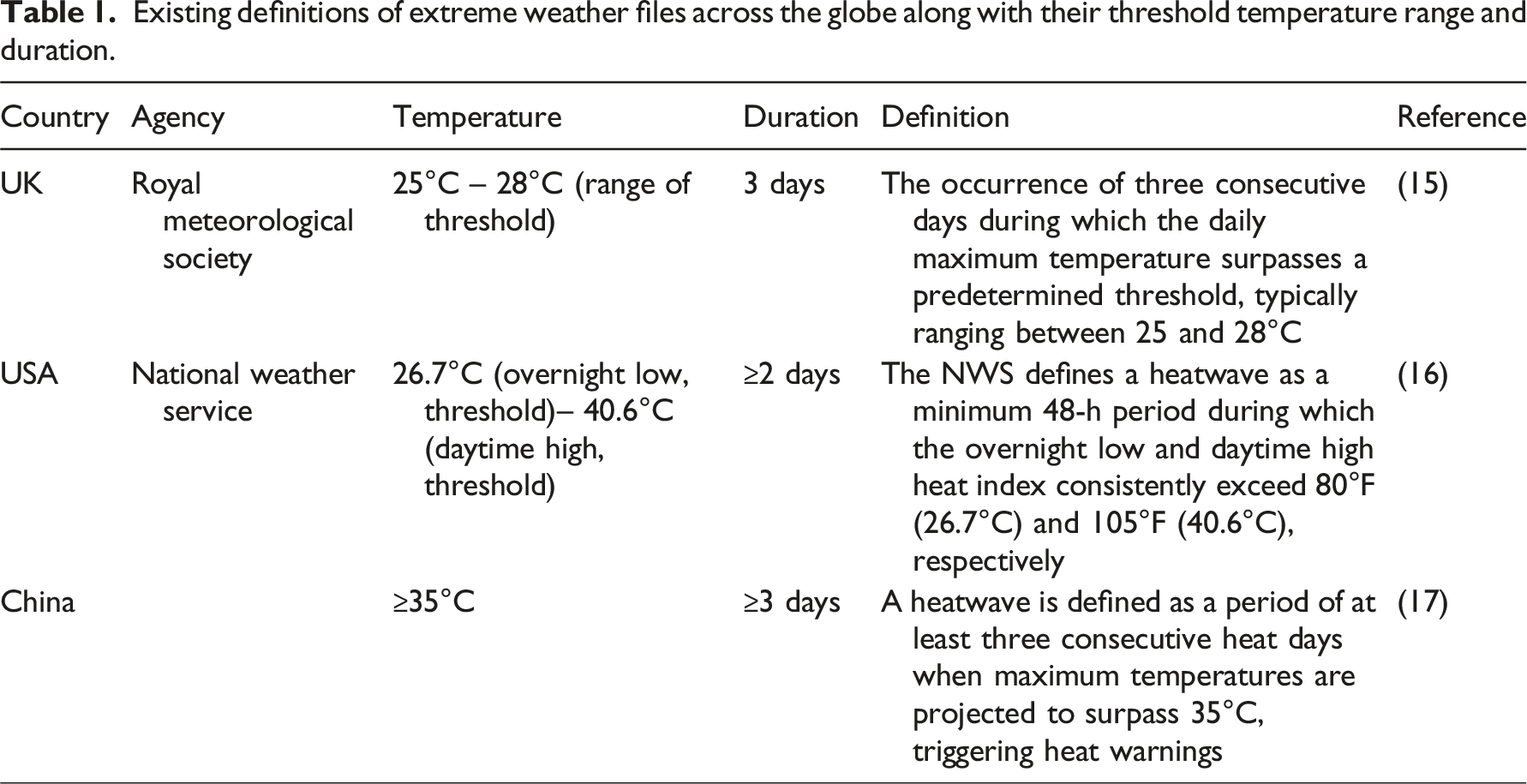
Existing definitions of extreme weather files across the globe along with their threshold temperature range and duration.

Country	Agency	Temperature	Duration	Definition	Reference
UK	Royal meteorological society	25°C – 28°C (range of threshold)	3 days	The occurrence of three consecutive days during which the daily maximum temperature surpasses a predetermined threshold, typically ranging between 25 and 28°C	(15)
USA	National weather service	26.7°C (overnight low, threshold)– 40.6°C (daytime high, threshold)	≥2 days	The NWS defines a heatwave as a minimum 48-h period during which the overnight low and daytime high heat index consistently exceed 80°F (26.7°C) and 105°F (40.6°C), respectively	(16)
China		≥35°C	≥3 days	A heatwave is defined as a period of at least three consecutive heat days when maximum temperatures are projected to surpass 35°C, triggering heat warnings	(17)

As this paper uses India as a case study of a large country with diverse climates, it is instructive to examine guidance for its extreme events in more detail. The guidance (see Table 2) covers differences due to topography (plains, hills, coast), day versus night time temperatures and severity (‘standard’ heat wave vs ‘severe’ heatwave).^18,19 However, there exist inconsistencies in publicly available definitions from different agencies. For example, the Indian Meteorological Department (IMD)’s FAQ defines a heat wave as a departure of maximum temperature from ‘normal’ by between 4.5 and 6.4°C; with ‘normal’ being defined as 40°C for the plains and 30°C for hilly regions. ¹⁸ If the excursion exceeds 6.4°C then it is declared a severe heat wave. The National Disaster Management Authority (NDMA) now broadly mirrors the above IMD guidance (removing inconsistencies with the temperature thresholds and minimum length of periods present in the earlier edition) though still omitting guidance on night time temperatures. Hence, different agencies within the same jurisdiction impute subtly different definitions.

Table 2.

The Indian Meteorological Department’s (IMD) criteria for heat waves and cold waves.

	Heat wave a	Cold wave
Based on departure	Threshold for departure b
Plains	Tmax, daily ≥ 40°C	Tmin, daily ≤ 10°C
Hilly regions	Tmax, daily ≥ 30°C	Tmin, daily ≤ 0°C
Coasts	Assumed as above	Assumed as above
	Magnitude of departure from threshold
“standard” c	+4.5°C to +6.4°C	−4.5°C to −6.4°C
severe	Exceeds +6.4°C	Exceeds −6.4°C
Based on actual temperature
“standard”	Tmax, daily ≥ 45°C	Tmin, daily ≤ 4°C (plains only)
severe	Tmax, daily ≥ 47°C	Tmin, daily ≤ 2°C (plains only)
Coasts, “standard”	Tmax, daily ≥ 37°C	Tmin, daily ≤ 15°C
Warm nights
	Threshold for departure
	Tmax, daily ≥ 40°C
	Magnitude of departure from threshold
Warm night	+4.5°C to + 6.4°C
Very warm night	Exceeds + 6.4°C

^a The heat wave criteria state that if the conditions set out above are met in at least two stations in a meteorological subdivision for at least two consecutive days, the event is declared on the second day. Similar guidance for cold waves does not seem to exist, but it would be reasonable to assume the same criteria apply.

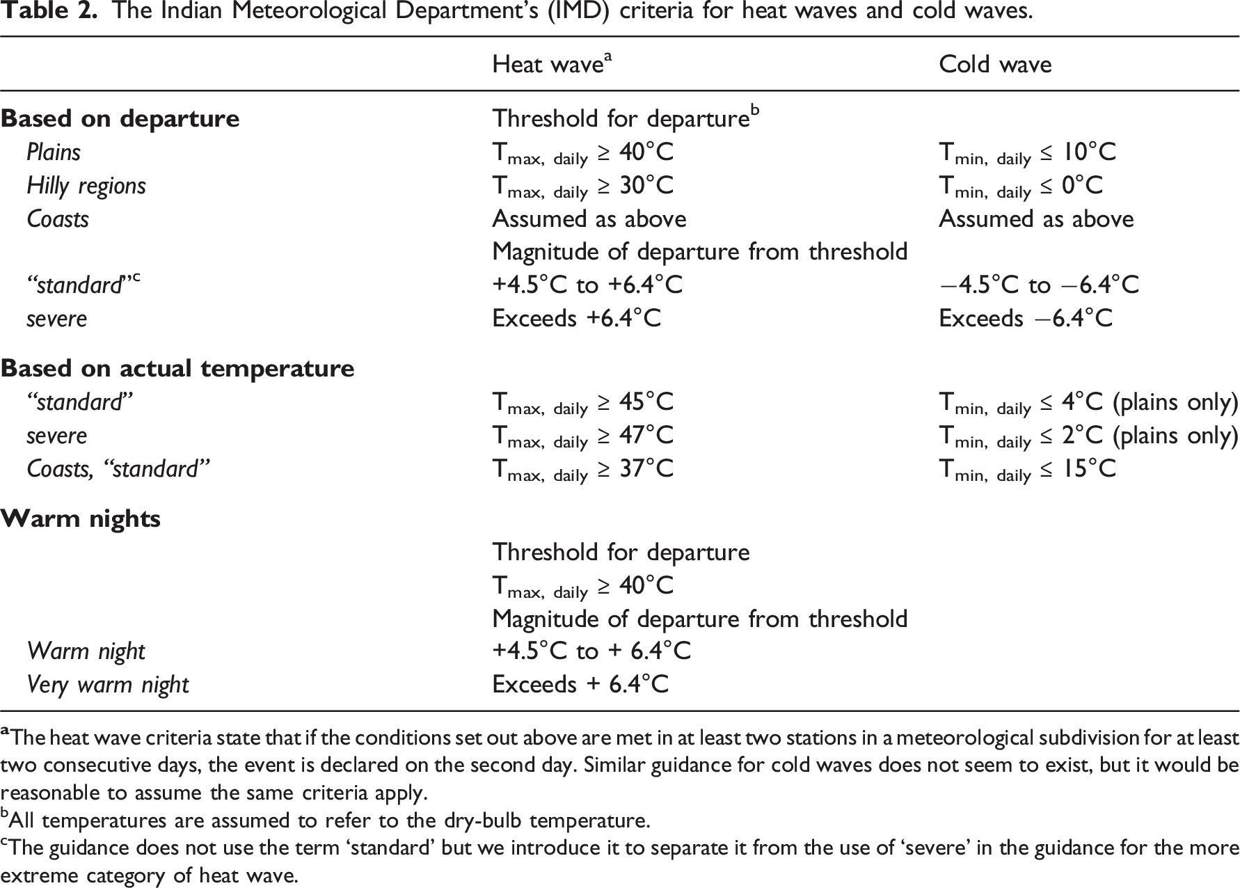
^bAll temperatures are assumed to refer to the dry-bulb temperature.

^cThe guidance does not use the term ‘standard’ but we introduce it to separate it from the use of ‘severe’ in the guidance for the more extreme category of heat wave.

The Indian Meteorological Department (IMD) definition for cold waves is similar to that of a heat wave and is reproduced in Table 2 and is broadly commensurate with the WMO definition, which defines a cold wave as “marked and unusually cold weather characterised by a sharp and significant drop in air temperatures near the surface (max, min, and daily average) over a large area and persisting below certain thresholds for at least two consecutive days during the cold season”.

Our key observation with respect to Table 2 (and under the National Disaster Management Authority (NDMA) guidance), is the use of absolute, potentially arbitrary, thresholds throughout. A similar situation exists in many other countries, for example, thresholds of 33°C in Korea, ²⁰ 40.6°C in the USA ¹⁶ and 28°C in the UK. ¹⁵ The existence of such wide ranging temperature thresholds is an implicit acknowledgement that human response to extreme events is strongly mediated by a localised experience of climate. Indeed, there is recent evidence that even the hypothesised ‘universal' physiological limit of 35°C wet-bulb temperature may not be universally applicable. ²¹ This suggests that what constitutes an extreme event for long-term residents of a given location is likely to differ from those of another location, with the difference being mediated by factors such as elevation, local water bodies and green cover. Further, one might reasonably expect that as the climate changes, new experiences will once again alter weather expectations in a community.

While the IMD guidance explicitly distinguishes by topography (plains, hills, coasts) as explained in Table 2, it does not allow a distinction within these categories. For example, plains in India might include parts of the desert regions of Thar in Rajasthan and riverine areas further to the east. Both are likely to experience significantly different climates and hence human expectations. Similarly, the well-known environmental lapse rate of a fall of between 0.6 and 0.9 °C every 100 m increase in elevation suggests that two hilly areas of different heights will likely experience different climates.

A second issue with the type of definition adopted by IMD, in common with many other countries, as discussed, is that humidity is implicit (through the definition of a different threshold for coasts) rather than explicit. Thus locations next to large water systems such as lakes and rivers will fall into one of the other categories (i.e. plains or hills). It also fails to account for differences in humidity arising from weather phenomena such as rainfall, particularly the monsoon, which, in India, is known to cause a significant seasonal elevation in humidity.

Finally, the criteria as set out are overlapping and could cause confusion. For example, for a location in the plains, the 40°C threshold being exceeded by 5°C automatically triggers the actual temperature threshold of 45°C suggesting the second criterion is not needed. Similarly, the setting of the warm night threshold to 40°C potentially isolates it to the ‘plains’ region. Thus, elevated night-time temperatures in the hills, where people can be hypothesised to be more sensitive to warm temperatures, would not trigger a heat wave warning when the daily maximum threshold of 40°C is not breached even if the temperatures are locally high, all the way to 39.9°C. Another source of confusion lies in the fact that while elevated night time temperatures are seen as a pressure-point in the heatwave guidance, no equivalent threshold is set for low day-time temperatures in the case of cold waves.

Recent studies, largely focused on heat waves, that have acknowledged some of these issue have proposed solutions that provide a means to localise events from a frequentist standpoint but lack the temporal detail (e.g. daily or hourly) that is often needed, especially in building simulators such as EnergyPlus. ²² They also do not consider the effect of the diurnal swing, preferring to use daily mean temperature or other factors such as humidity as the defining characteristic.

These issues suggest that a ‘universal’ definition of extreme events is needed that is both local and consistent. Such a definition would include the effect of a diurnal swing in temperatures such that high daytime and high night-time temperatures are considered together for a heatwave and, conversely, low daytime and low night-time temperatures are considered together for a cold wave.

In the next section, we examine whether existing definitions of extreme weather in the building simulation field meet these criteria.

Existing definitions for extreme weather for building simulation

A range of extreme weather formats presently exist for use in dynamic building simulation software, summarised in Table 3:

Table 3.

Existing approaches to generate extreme weather files with their intended goals and remarks.

S.No	Extreme weather file	Goal	Remarks
1	Probabilistic design summer year (pDSY)	To obtain weather files including events that could cause indoor overheating 23	This study proposes a method for determining return periods for warm weather events by considering a notional free-running building with operative temperatures mirroring outdoor temperatures and employs the static weighted cooling degree hours (SWCDH) to evaluate overheating. The identification of the design summer year (DSY) involves selecting the year with SWCDH return periods approximately equivalent to 7 years, marking it as a moderate event. Subsequently, more extreme summer years (pDSY) are identified based on their intensity or more prolonged overheating incidents compared to the moderate year. 23
2	Design reference year (DRY)	The DRY method is a systematic approach to generating hourly realistic, coincident design data from synthetic weather data (CP09) characterized by the inclusion of near-extreme values and occurrences of more prolonged consecutive days with heightened extremity. 24	The DRY generation process involves computing mean monthly air temperatures for each of the 3000 years, sorting them, and selecting a target year based on a chosen percentile (e.g., 87.5%). A 21-year band centred around this year is extracted from the CP09 daily weather file. Finkelstein–Schafer statistics are then calculated for daily mean temperatures, total daily solar irradiance, and mean daily relative humidity. The three years with the lowest combined rank sums, considering these parameters, are selected based on the closest mean monthly wind speed. This automated process ensures the extraction of extreme yet regionally representative data for design reference years (DRYs) in external air temperature, with analogous steps repeated for relative humidity and solar irradiance. 24
3	Summer reference year (SRY)	To facilitate summer overheating assessment of free-running buildings	The methodology employed for generating the SRY dry bulb temperature nodes involves a two-stage procedure. Initially, the 90th percentile warmest year is identified from the summer months (Apr to Sep) data spanning the TRY baseline years. Subsequently, a mathematical adjustment is applied to the hourly TRY data, aligning it with the identified candidate year representing the ‘high-temperature tail.' This adjustment adheres to the principle of a data shift, ensuring a refined representation of extreme temperature conditions. 8
5	Untypical meteorological year (UMY)	UMY weather files could be useful in the prediction of the maximum cost of building operations during severe winters and hot summers 25	The study introduces three untypical meteorological years (UMY v1, UMY v2, and UMY v3) derived from the WYEC2 reference years by employing distinct weighting indices. Among the nine parameters considered, the crucial factors in determining the composite index for UMY files are identified as minimum and maximum dry bulb temperatures, maximum wind speed, and daily total solar radiation. UMY v1 prioritizes nearly equal importance for maximum and minimum temperatures, daily solar radiation, and maximum wind speed. UMY v2 is characterized by extreme daily total solar radiation and dry bulb temperatures, while UMY v3 focuses on extreme wind speeds. The weighting indices for each type of UMY year are presented, and tailored for building performance simulations in Poland. 25
6	Hot summer year (HSY)	pHSY-1 (based on WCHD) could be used for assessing the severity and occurrence of overheating, while pHSY-2 (based on PET) could be used for evaluating thermal discomfort or heat stress. 26	pHSY-1 and pHSY-2 are employed to assess the risk of overheating and discomfort throughout the entire summer (Apr to Sep) rather than just during isolated heatwave events. This approach captures the cumulative impact of elevated temperatures. 26
7	Extreme reference year (ERYs)	The primary objective of utilising extreme reference year (ERY) weather files is to evaluate the energy resilience of buildings rather than serving as a source for determining design loads. The focus is on assessing the capability of buildings to withstand and adapt to variations in energy demands under extreme weather conditions. 27	The method is meant to be flexible and accommodating to generate different types of ERYs. This work focuses on building sensible heat balance, thus dry-bulb temperature and solar irradiance as weather variables are considered for extreme weather file generation. The ERYs are constructed on alternate hypotheses as opposed to the TRY weather file generation process. Months least representative of long-term distributions are identified and included in ERY. For instance, when evaluating building envelope performance, the ranking may be confined to DBT and GHI. 28
8	Extreme meteorological years (XMYs)	To capture a range of building performance and mitigate the influence of climate variability on decision-making. 29	For extreme meteorological years (XMY) in the process of selecting months, a comprehensive analysis of daily maximum, minimum, and average values for each relevant meteorological variable (e.g., dry-bulb temperature) over 15 years is carried out. The identification of extreme “daily” months involved scrutinizing daily maximum and minimum values for each day within a month. The month exhibiting the highest daily maximum value was designated as the maximum extreme, while the one with the lowest daily minimum value was assigned as the minimum extreme. For extreme “hourly” months, the average highest and lowest hourly values select the months, yielding four distinct combinations of possible extremes: Daily maximum, daily minimum, hourly maximum, and hourly minimum 29

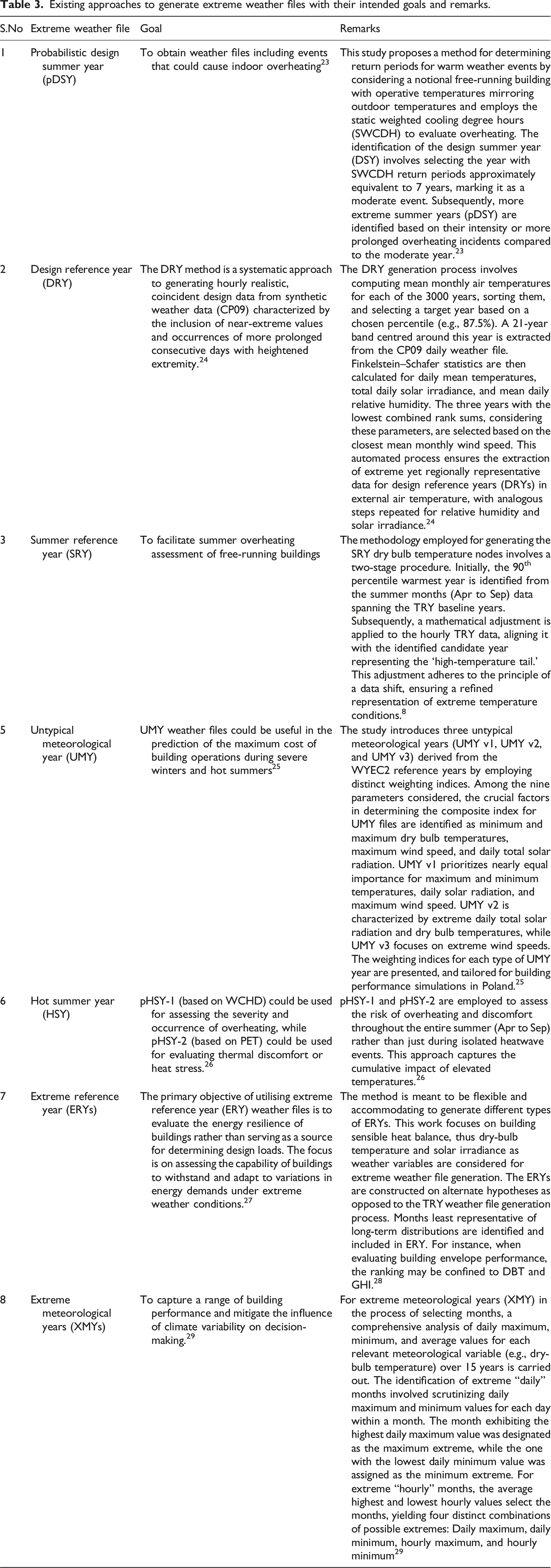
From Table 3 we observe that there are a variety of methods presently in existence to examine the impact of extreme periods on buildings. However, none of these methods explicitly set out to identify events of short duration, that is, heat waves and cold snaps. For example, the mean length of heat waves over 783 events in 164 cities distributed across 36 countries covering Europe, North America, Asia, Australia and Africa and occurring between 1980 and 2014 was 20 days. ³⁰ It is events of such duration that are needed for examining system resilience, whether for buildings or other aspects such as crop yield or outdoor health risk. In the case of buildings, the dynamic response is often to the order of an hour, which is also the usual timestep in the weather files shown in Table 3, matching the needs of simulators such as EnergyPlus. It is noteworthy that a period of extreme weather dominated by a single event (e.g. a single day) would be experienced very differently to a period of consistent extremeness, if the two have the same length and mean temperature. In case of the former, the system would be able to recover on the less extreme days whereas no such relief would be afforded in a period of consistent extremeness. Thus, it is critical to test resilience against the latter type of periods.

Our main aim is hence to develop a general method to embody localised short-duration extreme event signatures in a form that can be readily used for a variety of users studying climate resilience, but especially in building simulation. This requires the selection of suitable metrics, case-study data (India, in this instance), development and demonstration of the method, a comparison of the emergent extreme periods against the equivalent extremes in typical years and an illustration of the use of the new data in studying impacts. The rest of the paper hence follows this broad order.

Methods

As seen in Section 1, a method is needed to generate representations of extreme events consistent in definition but localised in the outcome. The events will have low diurnal swings, given that those with larger swings allow systems to recover, mitigating the impact of severity. Ideally, these representations will be simple to implement and interpret by various users.

We commence with the question of an appropriate metric: that is which weather variables would form part of an extreme event selection process. There are four key physical variables that inform the weather in a location: dry-bulb temperature, relative humidity, solar radiation and wind speed. Of these, the dry-bulb temperature is the most widely – and often the only – used metric, as seen earlier. There are several reasons for this. Firstly, it is seen as the main driving force for the response of a range of systems, especially buildings. This is connected to the second reason, being that many performance criteria use it either directly or through a derived indoor variable such as the use of operative temperatures in overheating assessment. ³¹ Thirdly, many weather stations record only temperature (and humidity) as solar radiation and wind speed often involve greater expense. Finally, temperature has a wide conceptual currency in public discourse, making descriptions of events based on temperature easily communicable. It would hence seem reasonable for any definition of an extreme event to use dry-bulb temperature.

Turning to the issue of humidity raised in Section 1.1, Figure 1 shows that humidity and temperature have a broad interdependence with locations of high relative humidity operating within a narrower band of air temperatures than those of dry locations. This would suggest that dry-bulb temperature alone could act as a proxy for humidity. While this would be true for long-term statistics, short-term events, even those of predictable periodicity, such as the monsoon, are outside the annual statistical norm for the location. One way to tackle this would be to evaluate extrema seasonally, but it would again require the imposition of arbitrary temporal boundaries, much like the temperature thresholds discussed earlier. Hence, some measure of humidity is needed.

Figure 1.

Density plots of daily maximum (bottom left) and daily minimum (bottom right) air temperature distributions from 201 tropical stations split by humid (120 locations comprising Köppen classes Af, Am, Aw and As) and dry (81 locations comprising BWh and BWk) climates. Data source: NCEI/NOAA weather database available at https://www1.ncdc.noaa.gov/pub/data/ghcn/daily/. The dataset contains daily air temperature data (max, min, average) from years spanning 1944 to 2016, though not all stations contain multi-year records.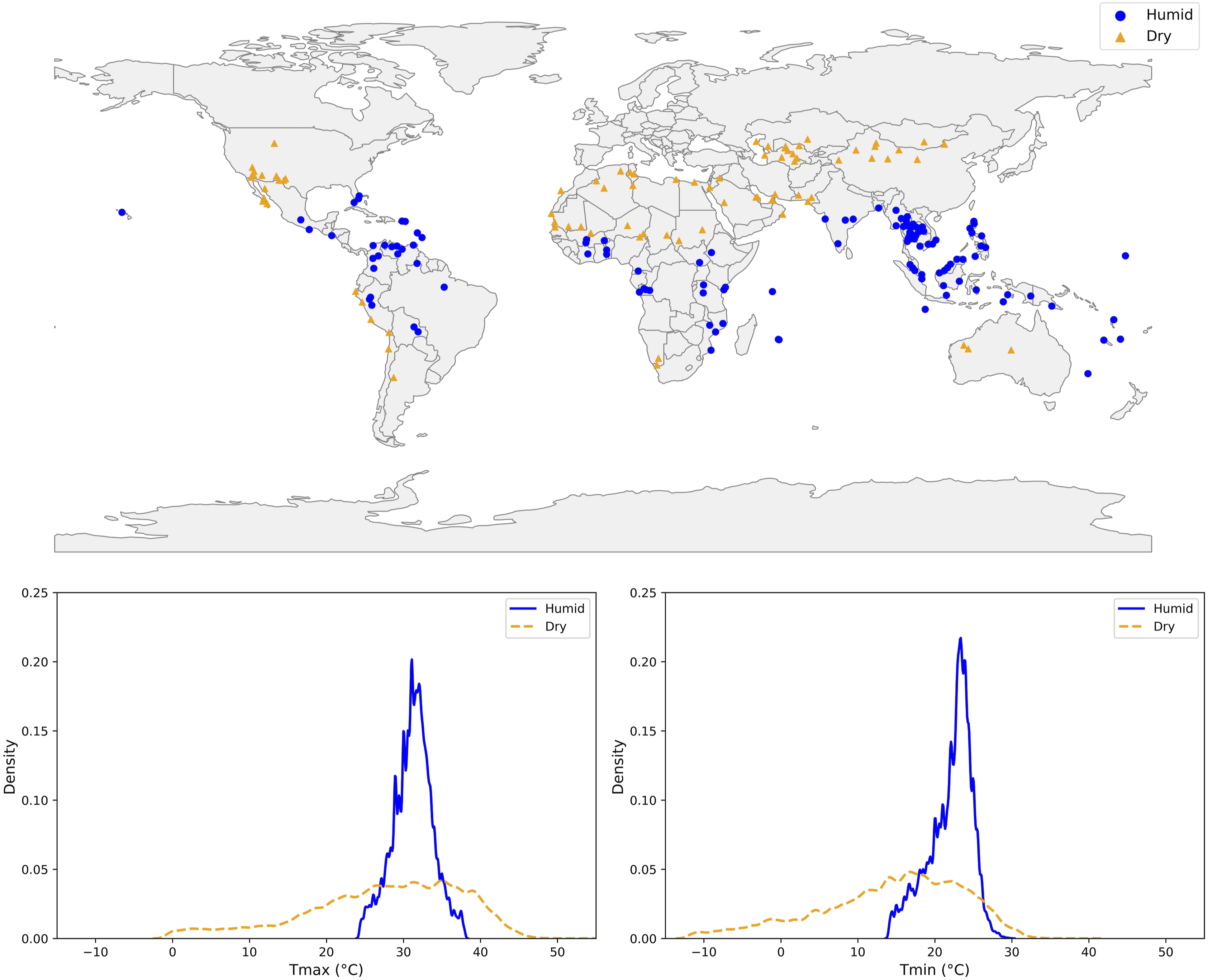

Wet-bulb temperature combines the effect of humidity and temperature and is the primary component (70% weighting) of the well-known wet-bulb globe temperature (WBGT) heat stress indicator. ³² Hence, the use of wet-bulb temperature extrema would allow easier identification of periods of heat stress, such as periods of the monsoon in India, through conversion into metrics such as the WBGT through the addition of globe and dry-bulb temperatures, and the Physiologically Equivalent Temperature (PET) etc. It would be equally as useful in determining cold stress, for example where low humidity and low air temperatures are known to increase risk of respiratory illness. ³³

Solar radiation and wind-speed can both be considered variables of additional interest as they act as vitiating or mitigating factors under extreme conditions.

It is hence clear that the selection of extreme events on the basis of extremes in dry-bulb and wet-bulb temperatures would be well grounded in current practice and the needs of various users, provided they were accompanied by other synoptic variables such as solar radiation and wind-speed to examine the effect of these vitiating or mitigating factors on overall risk.

We next consider method selection and any consequent data implications in the following two sections.

Extreme event selection

It is evident that the overall severity of the extreme event, critical in predicting morbidity and mortality in species or overall stress on energy systems, depends on both the intensity ³⁴ and duration ³⁵ of the event. In considering this, it is helpful to note that the goal of any extreme event representation is to enable stress-testing of systems when exposed to a realistic but extreme occurrence, with the view that a system capable of performing under such circumstances would also perform well under any event of lower severity. The following discussion is based on descriptions of a heat wave but the equivalent arguments for a cold wave will hold by reversing maxima with minima etc.

The key characteristics of a heat wave would be as follows:

1. Intensity: The selection of intensity is determined by the extent of deviation in dry and wet-bulb temperatures of a given period from the local norm.

2. Duration: For an event to count as a “wave”, it must occur for at least 2 days. The literature offers integer-increment event lengths between two and 10 days. ³⁴ However, in considering the ideal length of heat waves, it has been observed that a 7-day length is seldom exceeded in a variety of heat wave events and has inherent meaning within professional and public discourse. ³⁶ Thus, a 7-day event length meets the criterion of a realistic but extreme occurrence of a stress test.

3. Form: A wave with ‘peaky’ characteristics where daily maxima vary significantly over the wave, especially if accompanied by varying daily minima, will mean that system response will not be consistently stress-tested over the wave period, as discussed earlier. Hence, to fulfil the goal of stress-testing systems, we need each day in the wave to look similar to the others, that is, we wish to minimise the variance of the daily maxima and the diurnal temperature variation over the event.

From the above, we posit that extreme events designed for realistic stress testing ideally have a significant deviation from local norms, a week in length and each day similar to the other with a low diurnal temperature variation.

Data

Globally, continuous hourly synoptic observed weather data is scarce. In the UK, historical data of sufficient quality and length for generating typical weather has only been available for 14 locations ³⁷ or a grid spacing of about 132 km, assuming even spacing. Similarly, India has typical weather files generated only for 59 locations or 236 km grid spacing, noted earlier in Section 1. Fortunately, the generation of reliable synthetic weather data that meets these needs is now possible at the required spatio-temporal scale. While a deeper review of the different methods of generating synthetic weather data, including weather generators, is available elsewhere, ⁷ what is pertinent here is the observation that most synthetic generators are trained on historic data, which are limited in scope and availability. Hence a limitation of synthetic weather is that data are generated on station-scale and once converted into a grid format, the extremes are likely to be poorly represented. This, it is suggested in the preceding review, can be overcome through the use of Global Climate Model (GCM) data dynamically downscaled using a regional climate model which is more likely to produce a variety of extremes.

At present, weather generators, such as the UKCP09 used in UK work^7,38 are known to not accurately reproduce critical elements of Indian weather patterns such as the Indian monsoon. ³⁹ To overcome this, we instead use outputs from the UK Met Office’s Providing REgional Climates for Impacts Studies (PRECIS).^40,41 While newer models now exist, the model underlying PRECIS is well-regarded with an equilibrium climate sensitivity of 3.3°C very close to the multi-model mean (3.2°C, range 2.1 to 4.4°C) including against some newer models (Table 8.2 in ⁴² ), in wide use (e.g. ⁴³ ) with good performance for extremes.^44,45 PRECIS is a 17-member perturbed-physics ensemble climatic model in which the GCM HadCM3Q0-Q16 is downscaled to a 25 km resolution over India, thus producing a 130-year dataset (1970-2099) of hourly weather data. Future data within this PRECIS output are generated on the IPCC “Medium-High” A1B scenario, which envisions rapid economic growth, globalisation, rapid adoption of new and more efficient technologies, and a balance between fossil and renewable energy sources. The IPCC A1B scenario lies somewhere between the newer Reference Concentration Pathways (RCP) 4.5 and RCP 6.^46,47 We thus obtain 17 realisations of weather data over 130 years or 2210 years of continuous data. The data cover dry bulb temperature (°C), relative humidity ( $\%$ ), atmospheric pressure (Pa), horizontal infrared irradiance from the sky (W/m²), global horizontal radiation (Wh/m²), direct normal radiation (Wh/m²), diffuse horizontal radiation (Wh/m²), wind speed (m/s), wind direction (degree), Total sky cover (deca) and snow depth (cm). The calibration of these data for India using lower spatio-temporal resolution observed data from IMD is covered in a separate paper regarding the generation of Test Reference Years (TRY) ⁴⁸ but is summarised in Online Appendix A.

Event generation process

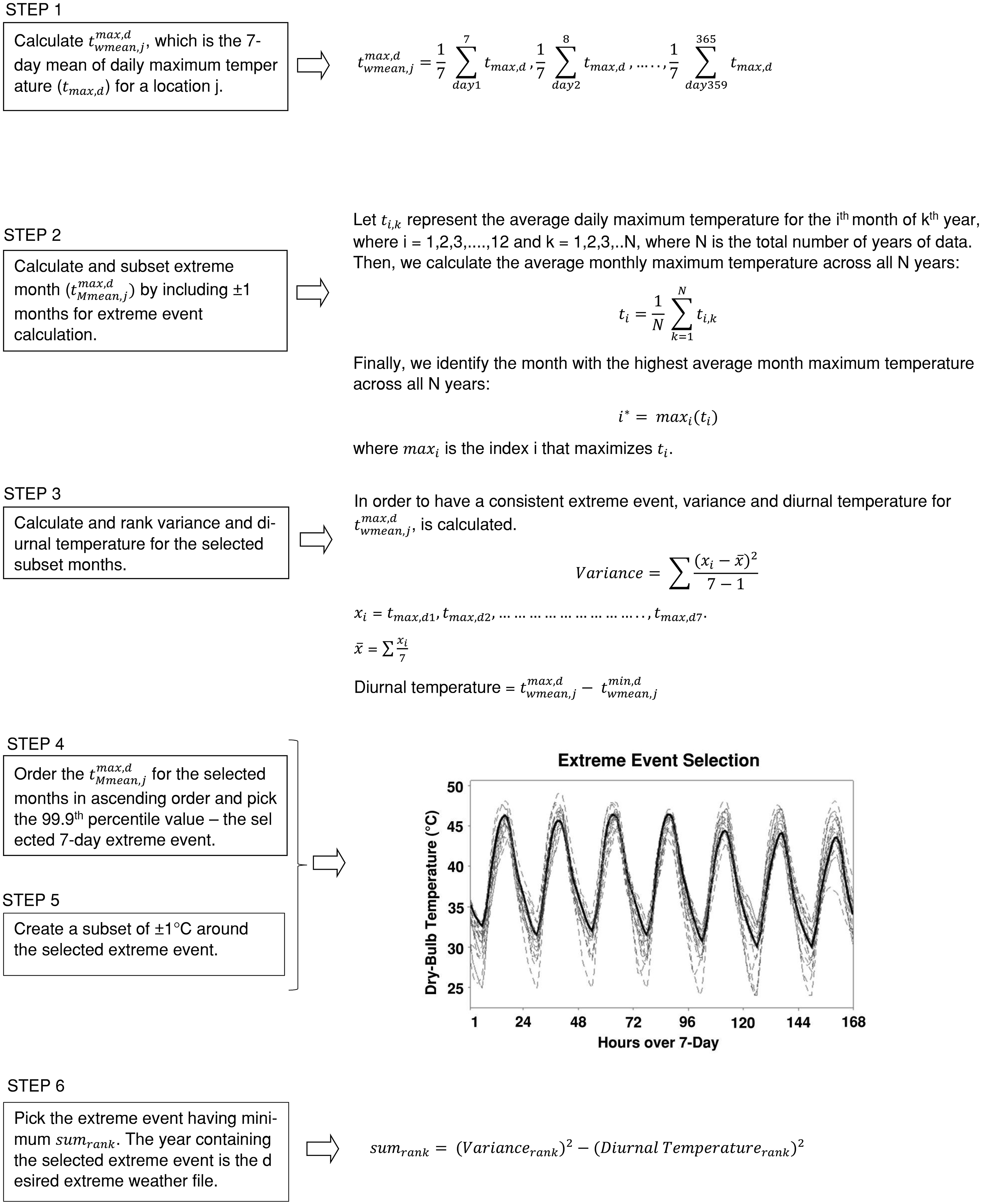
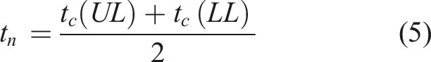
In determining the base period from which to draw our extreme week, we use the historical period 1981-2010 as there are summary statistics of observed weather for 400 stations from the IMD, ⁴⁹ including hot and cold temperature extremes, for much of the key variables over this period with which to perform a sense check. The same data were also used in the calibration process summarised in Online Appendix A. For future data, we use the period 2060 - 2089. In each period there are 510 (30 × 17) years of data. The steps are shown below and visually illustrated in Figure 3. These steps illustrate the procedure for heatwaves based on dry-bulb temperature. However, an equivalent process is applied for wet-bulb heat waves and dry-bulb cold waves, the latter by replacing with minimum temperatures as appropriate. We compute wet-bulb temperature (T_w) from dry-bulb temperature (T) and relative humidity (RH%) using the following equation ⁵⁰ :

$T_w=T\hspace{0.17em}\mathrm{atan}\left[0.151977{\left(RH\%+8.313659\right)}^{\frac{1}{2}}\right]+\mathrm{atan}\left(T+RH\%\right)-\mathrm{atan}\left(RH\%-1.676331\right)+0.00391838{\left(RH\%\right)}^{3/2}\mathrm{atan}\left(0.023101RH\%\right)-4.686035.$

(1)

• STEP 1. For each year we extract $T_{wmean,j}^{dmax}$ , which is the n-day (wmean) running mean of the daily maximum temperature (dmax) in a given location j. In the case of a 7-day event, this creates a dataset of 358 means × 30 years × 17 ensembles = 182,580 values. Illustrative values in the following steps also assume a 7-day event length.

• STEP 2. To minimise the search space to identify the event, we find the month with the highest mean temperature across all 510 years and choose a search space of ±1 month on either side of this. We hence reduce the search space for $T_{wmean,j}^{dmax}$ to 45,645 values. Within the above search window, we compute and rank the variance of daily maxima and diurnal temperatures.

• STEP 3. We rank order $T_{wmean,j}^{dmax}$ , and pick the event of the desired extremeness.

• STEP 4. This event represents the target but to identify an event with the desired minimised variance in maximum temperatures and diurnal swings, we create a new search space in $T_{wmean,j}^{dmax}$ that is ± 1°C on either side of this event.

• STEP 5. We now pick the entire year containing the event with the least sum rank of variance in daily maxima and diurnal temperature variation (obtained by summing the squares of both terms) within the search space created in the previous step.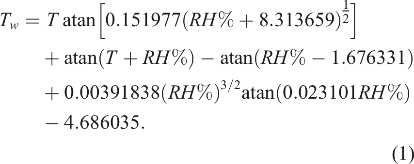

To determine the optimal number of days for event length, we analyse 3, 5, 7, 10 and 15-day event lengths (Figure 2). These data show that the extremeness of the selected events is inversely dependent on event length. We choose a 7-day duration for the reasons given in Section 2.1.

Figure 2.

Three to 15-day extreme event analysis for 59 locations representative of the locations currently in use for India via the ISHRAE data set. ¹⁰

Figure 3.

Illustration of the method.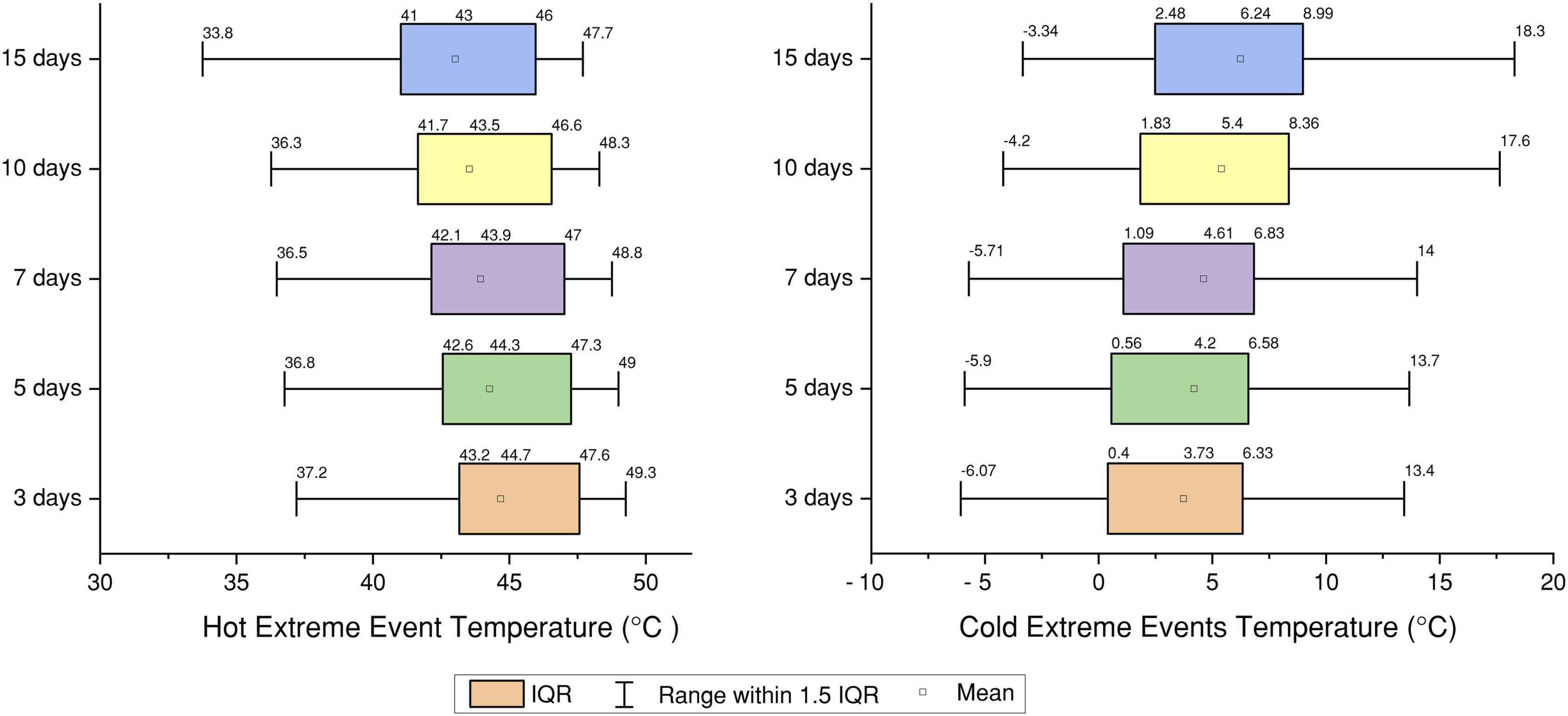

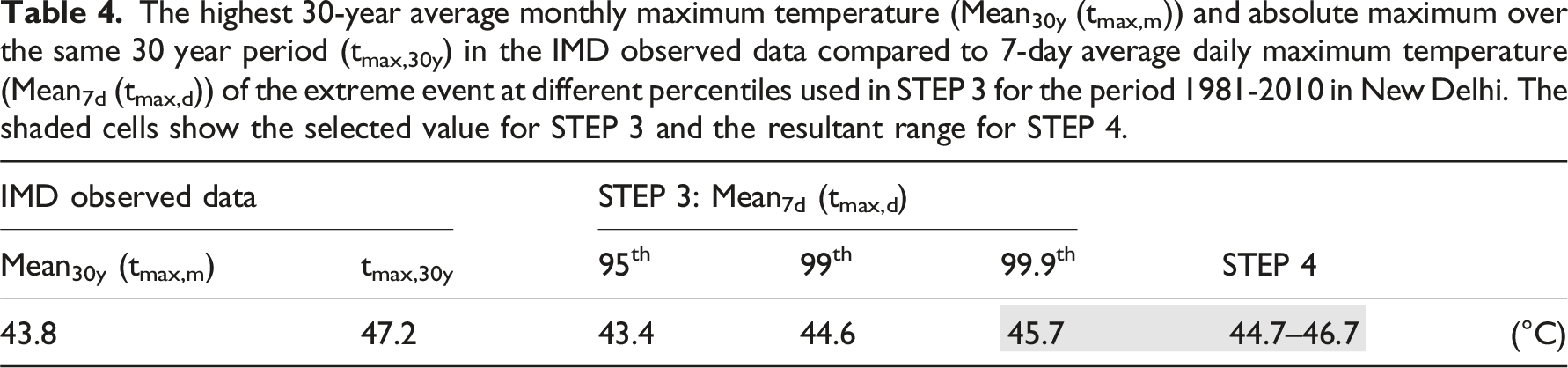
Next, to determine the desired extremeness for STEP 3, we have two possible values from the IMD dataset to give us a sense check against any selected thresholds. One, the 30-year mean of the monthly maximum temperature (i.e. mean_30y (t_max,m)), from which we can select the highest value (i.e. max of 12 values). The second is the absolute maximum observed over the 30-year (t_max,30). Exploratory analysis suggested that the 99.9^th percentile threshold (i.e. leaving a temperature tail of 183 events in $T_{wmean,j}^{dmax}$ ), produced a threshold sufficiently away from max (mean_30y (t_max,m)) such that the upper limit of the ±1°C range chosen in STEP 4 was close to t_max,30. Table 4 shows what this looks like for the example location of New Delhi (28.6° N, 77.2° E) against the 95^th (tail length 9129) and 99^th (tail length 1826) thresholds. Note that for cold waves, the selected threshold translates to the 0.1^th percentile.

Table 4.

The highest 30-year average monthly maximum temperature (Mean_30y (t_max,m)) and absolute maximum over the same 30 year period (t_max,30y) in the IMD observed data compared to 7-day average daily maximum temperature (Mean_7d (t_max,d)) of the extreme event at different percentiles used in STEP 3 for the period 1981-2010 in New Delhi. The shaded cells show the selected value for STEP 3 and the resultant range for STEP 4.

IMD observed data		STEP 3: Mean7d (tmax,d)			STEP 4
Mean30y (tmax,m)	tmax,30y	95th	99th	99.9th
43.8	47.2	43.4	44.6	45.7	44.7–46.7	(°C)

Using this process, we generate three types of Indian Peak Year (IPY) weather files using the basis data described earlier:

1. IPY_hot,dry: a representation of an extreme hot and dry spell using DBT.

2. IPY_hot,wet: a representation of an extreme hot and humid spell using WBT.

3. IPY_cold: a representation of an extreme cold spell using DBT.

As we produce both historic (1981-2010) and future (2060-2089) files of the above types for each location, we obtain 4790 locations × 6 files per location = 28,740 weather files for the case of India.

Building model development and validation

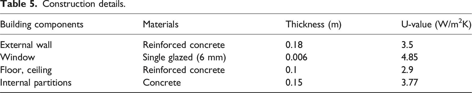
A residential building example is chosen to demonstrate the impact of our generated extreme events on indoor environments. The residential unit is situated on the 9^th floor of a 12-storey apartment within a gated community in the suburbs of Ahmedabad, thus representing typical middle-income housing through much of India. A thermodynamic model of a residential unit (Figure 4) is created in the widely used EnergyPlus software tool and calibrated using field data. The room is exposed to the south and east sides. The thermal performance of the residential unit was measured in terms of indoor dry-bulb temperature, globe temperature, relative humidity, air velocity and surface temperature of walls. Figure 4 illustrates the floor plan and the instrument locations used to measure and validate the simulation model and Table 5 provides construction details (further details in 51).

Figure 4.

(a) Floor plan and instrument locations and (b) instrument setup at Ahmedabad residence. ⁵¹ Calibration data for residential unit are used.

Table 5.

Construction details.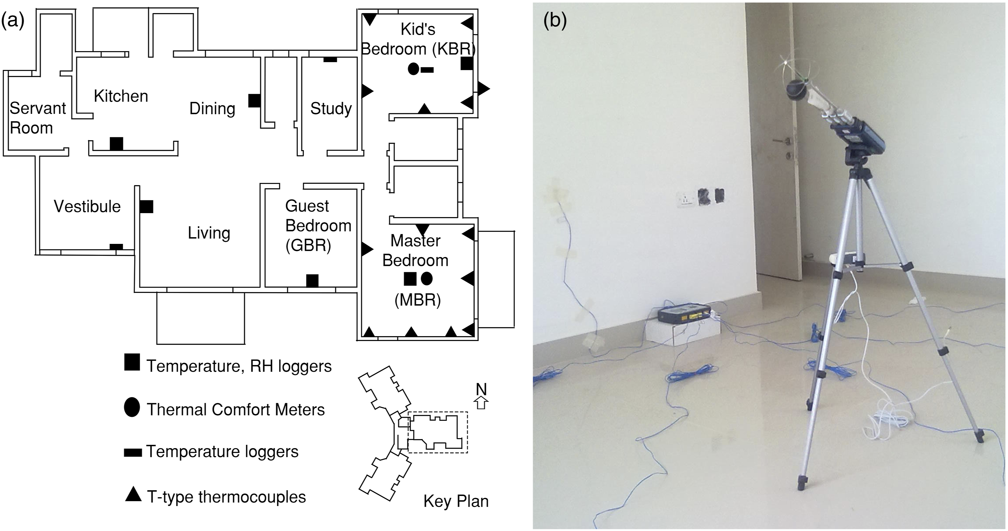

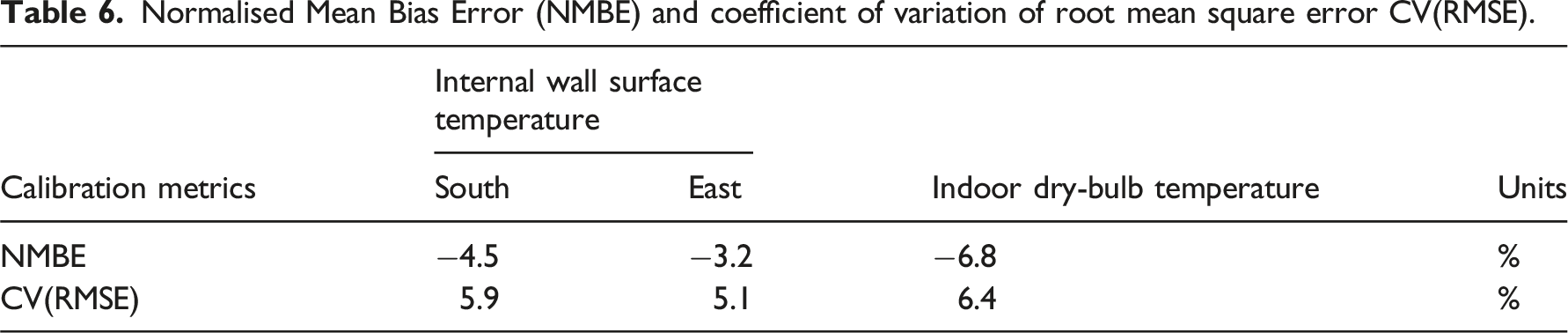
Building components	Materials	Thickness (m)	U-value (W/m2K)
External wall	Reinforced concrete	0.18	3.5
Window	Single glazed (6 mm)	0.006	4.85
Floor, ceiling	Reinforced concrete	0.1	2.9
Internal partitions	Concrete	0.15	3.77

Indoor data were collected for this study in 2012 and coincident external weather data were obtained. We use measured indoor dry-bulb temperature and wall surface temperatures to calibrate the building model (Table 6). ASHRAE considers model calibrated if the NMBE is within ±10% and CV(RMSE) is within ±30%. ⁵²

Table 6.

Normalised Mean Bias Error (NMBE) and coefficient of variation of root mean square error CV(RMSE).

Calibration metrics	Internal wall surface temperature		Indoor dry-bulb temperature	Units
	South	East
NMBE	−4.5	−3.2	−6.8	%
CV(RMSE)	5.9	5.1	6.4	%

Impact of the extreme event weather files on building performance

To explore the impact of the weather files created through the steps in Section 2.3, we subject the thermal model to the following scenarios:

1. Forensic: Taking the example of a single location with a humid subtropical climate (New Delhi, Cwa, ⁵³ we evaluate the indoor thermal performance of the model using a typical year (50^th percentile TRY: pTRY) and the corresponding three IPY weather files for historic climate. We identify comparator identical-length periods in the pTRY for each IPY type (i.e. the hottest dry and wet spells and the coldest spells in a typical year). We also compare historic IPYs (1981-2010) against future projection IPYs (2060-2089).

2. Spatiotemporal: we examine variations in indoor conditions between the historical period (1981-2010) and the prospective future period (2060-2089) for each type of IPY. These are considered alongside the variations in external conditions.

A total of 28,740 simulations (i.e. one per file in our newly created database) covering Indian Peak Year (IPYs) derived using dry-bulb and wet-bulb temperatures for the past (1981-2010) and the future (2060-2089) were performed. Annual simulations were conducted and data for the 7-day extreme event periods were extracted and processed using the R programming language (version 4.3.1) and the RStudio integrated development environment (version 2023.06.0 + 421 ″Mountain Hydrangea”) for Windows. QGIS (version 3.32.0) is used for spatial plotting at a resolution of 25 km × 25 km.

In addition to outdoor conditions, we are interested in the potential impact of these outdoor conditions on indoor temperatures, assuming unconditioned (i.e. free-running) operation. However, the cumulative effect of temperature excursions beyond the critical limits of thermal comfort is equally important, both as an indicator of thermal stress and potential space conditioning demand to mitigate such stress. Hence, we illustrate indoor performance using the 7-day mean (i.e. over the event) maximum ( ${\overline{t}}_{\mathit{max}}$ ) and minimum ( ${\overline{t}}_{\mathit{min}}$ ) dry-bulb temperatures.

Given that building occupants are likely to demonstrate climatic adaptation between historic and future climates, the critical limit for DDH is calculated using the running mean temperature (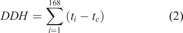 $t_{rm})$ during extreme events Equation (2). The neutral temperature (t_n) is calculated using the 90% acceptable operative temperature range as shown in Equations (3) and (4). ⁵⁴ Thus, the critical temperature considered to calculate DDH for IPY_hot is the localised ‘t_n’ (neutral temperature) value. In the case of IPY_cold, the critical limit of ‘t_n’ to calculate DDH is taken as 18°C as per WHO housing and health guidelines. ⁵⁵

$DDH={\displaystyle \sum }_{i=1}^{168}\left(t_i-t_c\right)$

(2)

$t_c\left(UL\right)=0.53\times \hspace{0.17em}{t}_{rm}+13.4+2.4$

(3)

$t_c\hspace{0.17em}\left(LL\right)=0.53\times \hspace{0.17em}{t}_{rm}+13.4-2.4$

(4)

$t_{n\hspace{0.17em}}=\frac{t_c\left(UL\right)+t_c\hspace{0.17em}\left(LL\right)\hspace{0.17em}}{2}$

(5)where t_i is the hourly DBT in the extreme event and t_c is the critical temperature for threshold limit. The adaptive thermal comfort limits ( $t_c\left(UL\right)$ upper and $t_c\hspace{0.17em}\left(LL\right)$ lower), for 7-day running mean temperature are considered per the Indian model of thermal comfort. ⁵⁴ The neutral temperature calculated for IPY_hot-dry and IPY_cold is used as the t_c (critical temperature) to calculate DDH. Since the adaptive thermal comfort model derives neutral temperature based on dry-bulb temperature, it cannot be used for calculating DDH for IPY_hot-wet. Therefore we use 29°C wet-bulb temperature as the limit to test IPY_hot-wet based on a moderate warm stress level in the Physiological Equivalent Temperature Index. ⁵⁶ This is also closely associated with the WBGT-based heat flag system by the US army which considers a yellow flag at 29.4°C. ⁵⁷ Note that positive values correspond to cooling DDH and negative values correspond to heating DDH.

Results

In this section, we describe our results and then validate our approach by docking our data against all known observed data. A second source of quality testing emanates from demonstrating a clear and significant deviation in the extremes selected through our procedure against the equivalent extreme period in a typical year for the same location and period.

Visualisation of IPY data

Figure 5 presents extreme event temperature values from IPYs of the past (1981-2010) and future (2060-2089) as a spatial raster with a pixel resolution of 25 km × 25 km. Our key observation is that the range of temperatures either contracts (DBT) or expands (WBT) slightly whilst experiencing a positive increase for both the lower and upper bounds. The WBT data are noteworthy for breaching the theoretical upper limit for 6-h exposure at 35°C, and well above the potential real limit of around 31°C. ²¹ Figure 5 subplots c and d also show higher IPY_hot-wet event values in the future than in the past in the Thar desert region of north-western India, consistent with. 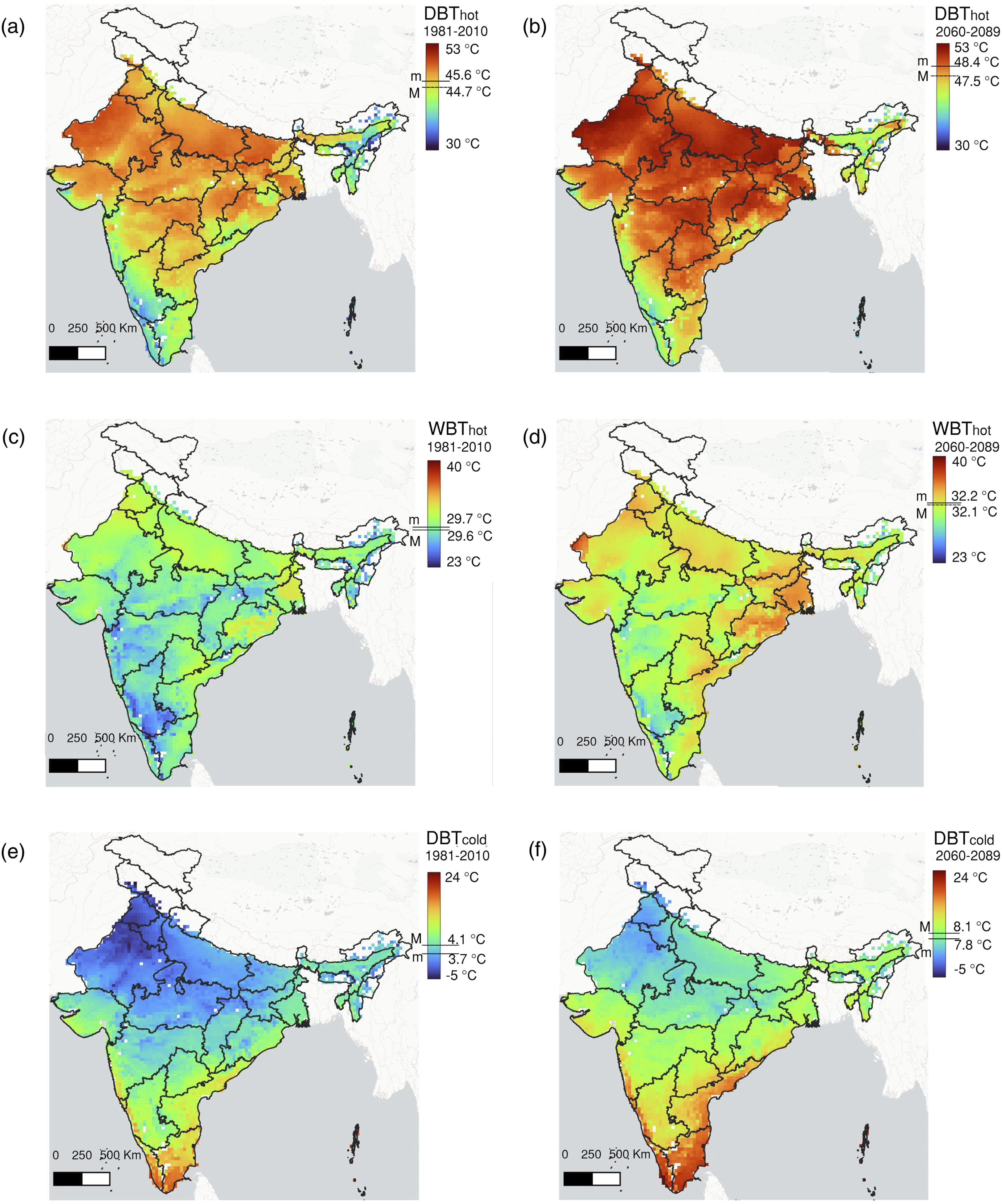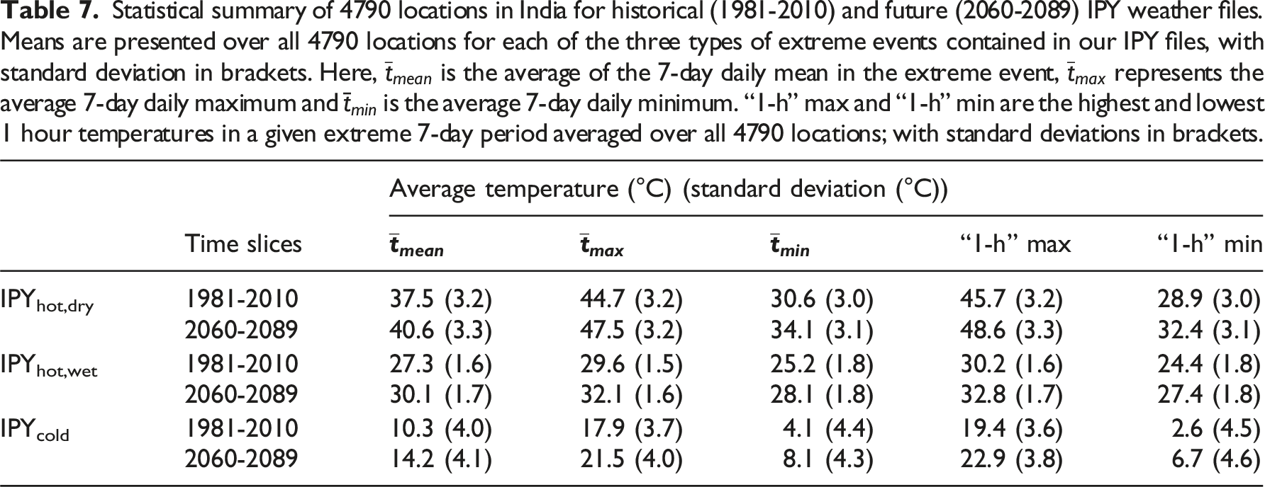⁵⁸ Mean DBT ${\overline{t}}_{\mathit{max}}$ above 50°C – that is likely well above this limit given a standard deviation of 0.5°C – for parts of a 7-day period also suggest the likelihood of extreme heat stress in parts of the country. The latter is observed to occur in 1114 locations in the future period (2060-2089), that is 21.2% of the country, whereas there is no location having mean DBT ${\overline{t}}_{\mathit{max}}$ above 50°C in the past (1981-2010).

Figure 5.

${\overline{\mathit{t}}}_{\mathit{min}\hspace{0.17em}/\hspace{0.17em}\mathit{max}}^{\mathit{e}\mathit{x}}$ for 4790 locations in India for the extreme event in the past (1981-2010) on the left and future (2060-2089) on the right for each extreme type. Here, (a) and (b) represent the mean daily maxima based for IPY_hot,dry; (c) and (d) represent the mean daily maxima for IPY_hot,wet; and (e) and (f) represent the mean daily minima for IPY_cold. ‘M’ stands for mean and ‘m’ for median. Areas with elevation >1000 m above mean sea level are in white due to lack of good basis data.

Statistical summary

Next, we briefly describe the broad statistical picture of the three generated file types and their characteristics in the two-time slices in Table 7. We observe that, on average, future dry-bulb temperatures for hot events are around 3°C warmer and for cold events about 4°C warmer, with the magnitude of standard deviations similar to these differences. Wet-bulb hot extremes are around 2.5°C warmer with standard deviations of around 1.6°C. The representative concentration pathways (RCPs) developed under the Coupled Model Inter-comparison Project 5 (CMIP5) suggest the mean warming in India is likely to be in the range of 3.3 °C–4.8°C (between RCP 6.0 and RCP 8.5 scenario) when the 2070s are compared to pre-industrial times, which is comparable to our PRECIS data here. ⁵⁹

Table 7.

Statistical summary of 4790 locations in India for historical (1981-2010) and future (2060-2089) IPY weather files. Means are presented over all 4790 locations for each of the three types of extreme events contained in our IPY files, with standard deviation in brackets. Here, ${\overline{t}}_{mean}$ is the average of the 7-day daily mean in the extreme event, ${\overline{t}}_{\mathit{max}}$ represents the average 7-day daily maximum and ${\overline{t}}_{\mathit{min}}$ is the average 7-day daily minimum. “1-h” max and “1-h” min are the highest and lowest 1 hour temperatures in a given extreme 7-day period averaged over all 4790 locations; with standard deviations in brackets.

	Time slices	Average temperature (°C) (standard deviation (°C))
		${\overline{\mathit{t}}}_{\mathit{m}\mathit{e}\mathit{a}\mathit{n}}$	${\overline{\mathit{t}}}_{\mathit{max}}$	${\overline{\mathit{t}}}_{\mathit{min}}$	“1-h” max	“1-h” min
IPYhot,dry	1981-2010	37.5 (3.2)	44.7 (3.2)	30.6 (3.0)	45.7 (3.2)	28.9 (3.0)
	2060-2089	40.6 (3.3)	47.5 (3.2)	34.1 (3.1)	48.6 (3.3)	32.4 (3.1)
IPYhot,wet	1981-2010	27.3 (1.6)	29.6 (1.5)	25.2 (1.8)	30.2 (1.6)	24.4 (1.8)
	2060-2089	30.1 (1.7)	32.1 (1.6)	28.1 (1.8)	32.8 (1.7)	27.4 (1.8)
IPYcold	1981-2010	10.3 (4.0)	17.9 (3.7)	4.1 (4.4)	19.4 (3.6)	2.6 (4.5)
	2060-2089	14.2 (4.1)	21.5 (4.0)	8.1 (4.3)	22.9 (3.8)	6.7 (4.6)

Quality testing

Here we present three different quality measures for the produced data involving validation, self-consistency and temporal consistency.

Validation

The IMD dataset carries information on extreme data for many locations, with some stations stretching back more than 150 years. The earliest established station was in 1792, with data being collected from Chennai (Nungambakkam), and the most recent station was established in 1995 at Tuni (Andhra Pradesh). The mean bias error between the maximum dry-bulb temperature in our DBT_hot week for the historical period against the long-term ‘peak maximum’ temperature for the hottest month in the IMD record is + 0.2°C (sd = 2.4°C). A two-sample Kolmogorov-Smirnov test does not suggest a significant difference between the distributions of (n = 332 for both groups, D = 0.099, p = .075). The mean bias error for the DBT_cold week and corresponding historical data is + 1.8°C (sd 2.5°C, n = 324, D = 0.197, p = .000), suggesting the cold extrema distributions are not drawn from the same distributions. Overall, however, with cold extrema becoming less significant over time, the data suggest the extreme weeks from PRECIS are a good representation of historically experienced extremes.

We also examine the 30-year mean monthly extreme for the month containing the selected event in our data to match its counterpart mean monthly extreme in the IMD dataset (Figure 6). Although there may not always be a one-to-one correspondence between the month containing the extreme event and the most extreme month in the IMD dataset, we always select the ‘hottest’ IMD month as comparator as our goal is to broadly compare the representativeness of the month containing the extreme against known historical data. For example, for Roorkee city, the selected event is contained in May which has an average monthly maximum of 43.2°C (i.e., we compute the average for the “1 hour” May monthly maxima for 30 years × 17 ensembles) whereas IMD recorded a mean monthly maximum of 42.3°C for June (i.e., the mean of “1 hour” monthly maxima recorded over 30 years, 1981-2010). ⁴⁹ Note that, unlike their dry-bulb equivalents, wet-bulb extrema are not contained in the IMD source. Instead, morning and afternoon monthly averaged daily values are available, as shown.

Figure 6.

Distribution of temperature differences between PRECIS and IMD. Positive values indicate PRECIS > IMD. ∆DBT_hot = difference in monthly average daily maximum dry-bulb temperatures of the hottest month (n = 339); ∆DBT_cold = difference in monthly average daily minimum dry-bulb temperatures of the coldest month for (n = 330); and differences in monthly average daily mean wet-bulb temperatures for morning (∆WBT_hot(m)) and evening (∆WBT_hot(e)) of the hottest month (n = 322).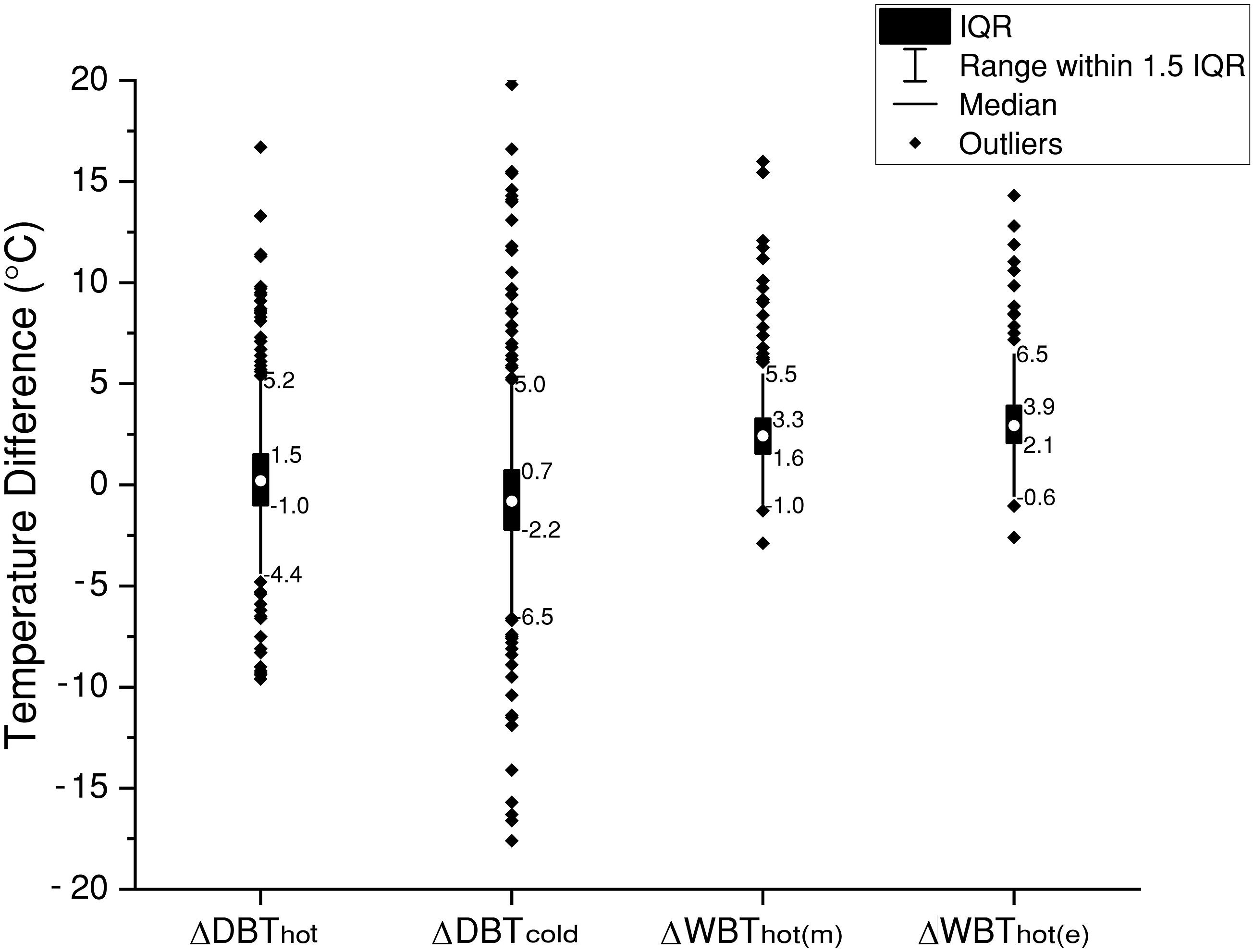

We observe that PRECIS demonstrates a good degree of agreement with observed data from IMD, though there are some significant deviations around the tail of the distributions and some large outliers. This broad agreement substantiates the model’s ability to replicate historical statistical patterns.

Self-consistency

Previous work in the UK has shown that the selection process for a Design Summer Year (DSY, a warmer than average year in 30 years) can produce a cooler summer than the summer in the equivalent Test Reference Year (TRY, a typical year in the same 30 year period), ⁶⁰ later corrected in 23. The equivalent problem here is that a TRY contains a 7-day period of weather that is more extreme than the selected week in the IPY file. Table 8 hence compares the extreme weeks in our IPYs with the equivalent period in our 50^th percentile typical reference year (pTRY₅₀) file, the latter being the subject of a separate paper ⁴⁸ to identify cases of such unexpected behaviour for three key metrics, individually and in combination: ∆ ${\overline{t}}_{mean}$ , ∆ ${\overline{t}}_{\mathit{max}}$ and ∆ ${\overline{t}}_{\mathit{min}}$ (see explanations in Table 8). The maximum ‘error rate’ occurs for ∆ ${\overline{t}}_{\mathit{max}}$ for IPY_hot-wet with 214 locations – that is 4.5% of the locations in our dataset show a TRY file 7-day mean maximum wet-bulb temperature in excess of that picked up in the IPY file. Only 26 locations or just 0.5% of the 4790 locations show unexpected behaviour for all three metrics. Most of these are in northeast India, close to a water body, a hill range, or both. We show how this issue can be resolved by taking any of the eight adjacent locations around the poorest-performing locations at 25 km × 25 km resolution in Online Appendix B. The distribution of differences for all three metrics is presented in Online Appendix C.

Table 8.

The error rate, that is number of locations where the extreme week in an IPY is less extreme than the most extreme week in a typical year in the same period (pTRY₅₀) for all 4790 locations. We measure the error rate by comparing, in isolation, weekly mean (∆ ${\overline{\mathit{t}}}_{\mathit{m}\mathit{e}\mathit{a}\mathit{n}}$ ), mean maximum (∆ ${\overline{\mathit{t}}}_{\mathit{max}}$ ) and mean minimum (∆ ${\overline{\mathit{t}}}_{\mathit{min}}$ ), dry and wet-bulb temperatures, as appropriate. In addition, we look at locations where any two and finally all of these three metrics do not perform as expected. Blank cells = 0 locations.

	Time slices	(°C)
		∆ ${\overline{\mathit{t}}}_{\mathit{m}\mathit{e}\mathit{a}\mathit{n}}$ only	∆ ${\overline{\mathit{t}}}_{\mathit{min}}$ only	∆ ${\overline{\mathit{t}}}_{\mathit{max}}$ only	∆ ${\overline{\mathit{t}}}_{\mathit{m}\mathit{e}\mathit{a}\mathit{n}}$ and ∆ ${\overline{\mathit{t}}}_{\mathit{min}}$	∆ ${\overline{\mathit{t}}}_{\mathit{m}\mathit{e}\mathit{a}\mathit{n}}$ and ∆ ${\overline{\mathit{t}}}_{\mathit{max}}$	∆ ${\overline{\mathit{t}}}_{\mathit{min}}$ and ∆ ${\overline{\mathit{t}}}_{\mathit{max}}$	∆ ${\overline{\mathit{t}}}_{\mathit{m}\mathit{e}\mathit{a}\mathit{n}}$ and ∆ ${\overline{\mathit{t}}}_{\mathit{min}}$ and ∆ ${\overline{\mathit{t}}}_{\mathit{max}}$
IPYhot,dry	1981-2010		44	31	17	7	8	5
	2060-2089		38	20	7	5	3	3
IPYhot,wet	1981-2010		33	165	29	64	6	5
	2060-2089		18	214	22	66	13	13
IPYcold	1981-2010		4	7
	2060-2089			9		1

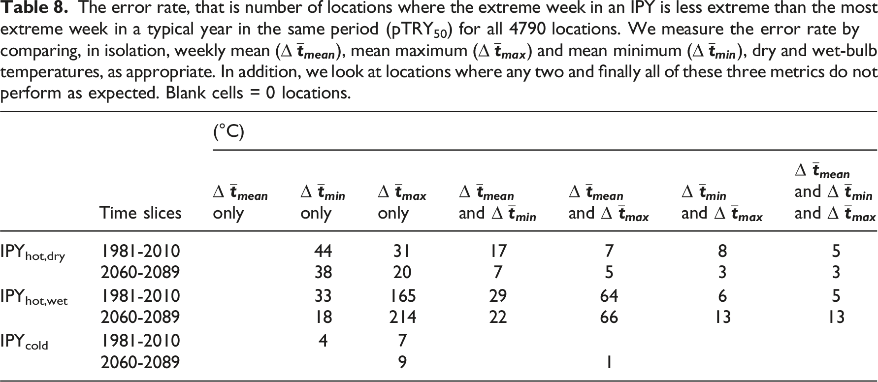
To aid user judgment of data quality, we encode the above information in the IPY file’s comment fields, which is part of the standardised EPW format, as follows (with examples drawn from the 1981 – 2010 IPY-hot DBT file for New Delhi):

COMMENT 1. : Extreme 7-day hot period starts on day 156/365 (5 Jun 1982, PRECIS Ensemble Number 5). Mean dry bulb temperature = 38.6°C, mean daily t_max = 45.7°C, mean daily t_min = 31.6°C.

COMMENT 2. : How much hotter is this period than the hottest 7-day period in the matching 50th percentile pTRY? Delta mean dry bulb temperature = 2°C, delta mean t_period_max = 2.8°C, delta mean t_period_min = 1.2°C.

Temporal consistency

Our event selection process is broadly agnostic to the time of year and it is hence likely that, when examining differences in performance, the comparators available to a designer are not temporally coincident. For example, sun paths in May will be different to those in June and hence comparing an IPY from the 1990s occurring in May with one occurring in July in the 2080s may present analytical challenges to the designer. Hence, if an extreme week occurs in the first week of May in the 1990s, it would be ideal if the corresponding extreme week in the 2080s also occurred on the first week of May. To find out how often this happens and the scale of deviation when it does not, Figure 7 shows a histogram of the deviation of events of interest from a series of possible baseline comparators.

Figure 7.

Histograms of the differences in number of days selected in our 7-day extreme events. Differences are measured from the start of each event. The left column (blue) histograms represent difference between future (2060-2089) and past (1981-2010) IPY events (past = 0). The right side histograms represent difference in IPY events against the equivalent 7-day period in the pTRYs (pTRY₅₀ = 0). Each panel shows the percentage of data contained within ±30 days.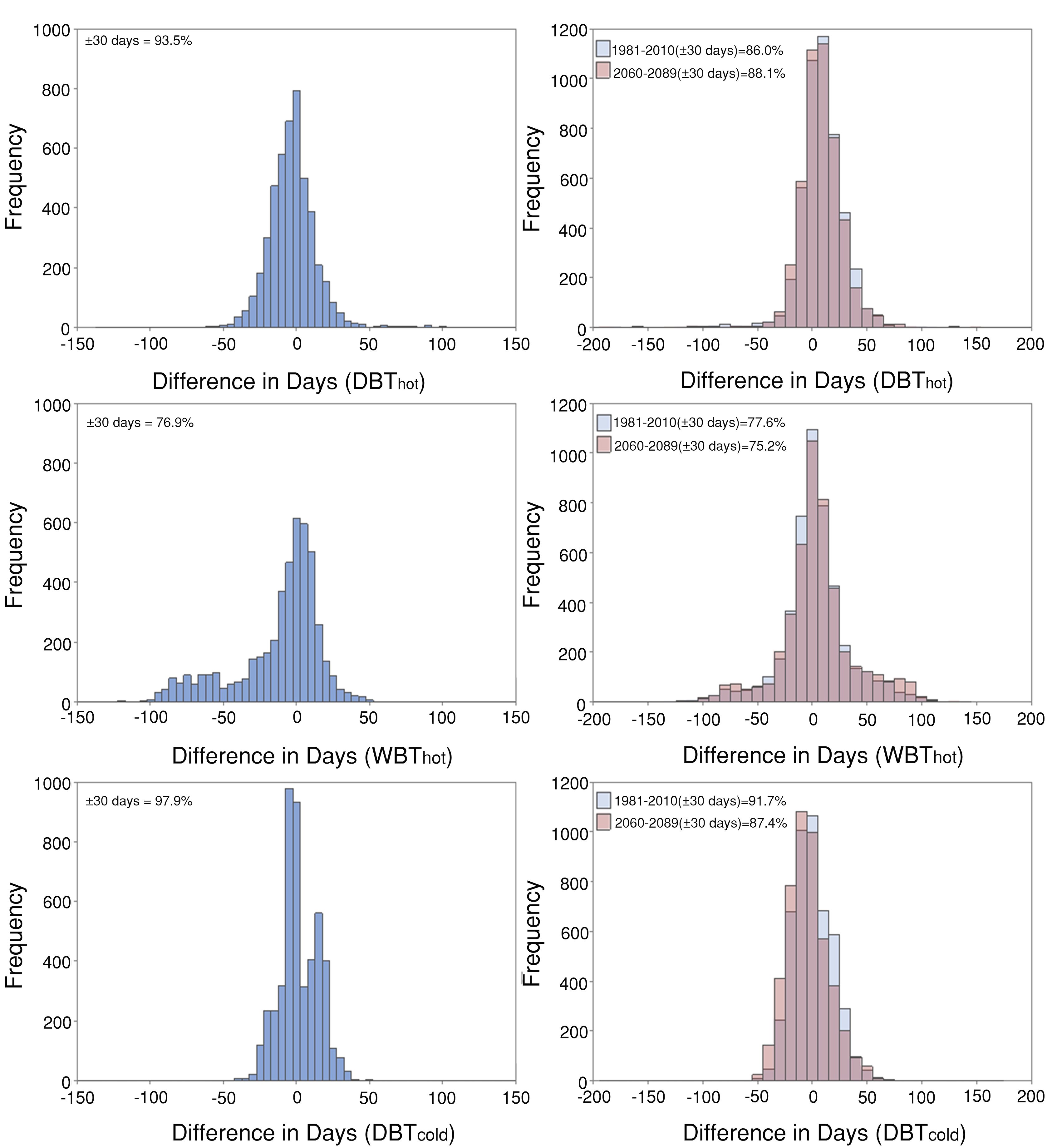

In general, we find strong temporal consistency across the comparators in Figure 7, with 86% of all data lying between ±30 days and 60.9% of data between ±15 days. Changes in WBThot event timing are apparent with future events tending to occur earlier in the year compared to the past in a minority of locations (Figure 7, left-middle) and these being occasionally distinct from their pTRY counterparts (Figure 7, right-middle).

Impact of extreme events on indoor thermal environment

The forensic evaluation discussed in Section 2.5 is shown in Figure 8 and Table 9 for each IPY “extreme event” type comparing to its corresponding pTRY₅₀ extreme event for the humid subtropical climate of New Delhi for the residential unit detailed in Section 2.4.

Figure 8.

Time series of indoor temperature for IPYs and TRYs for past (1981-2010) and the future (2060-2089), New Delhi simulated for the residential unit shown in Section 2.4.

Table 9.

Comparison between pTRY₅₀ and IPYs in terms of 7-day indoor means of daily maxima and minima and Degree-weighted Discomfort Hours (DDH) for the case of New Delhi. Note that pTRY DDH are shown as absolutes to simplify reading. Temperatures in brackets are critical thresholds for DDH.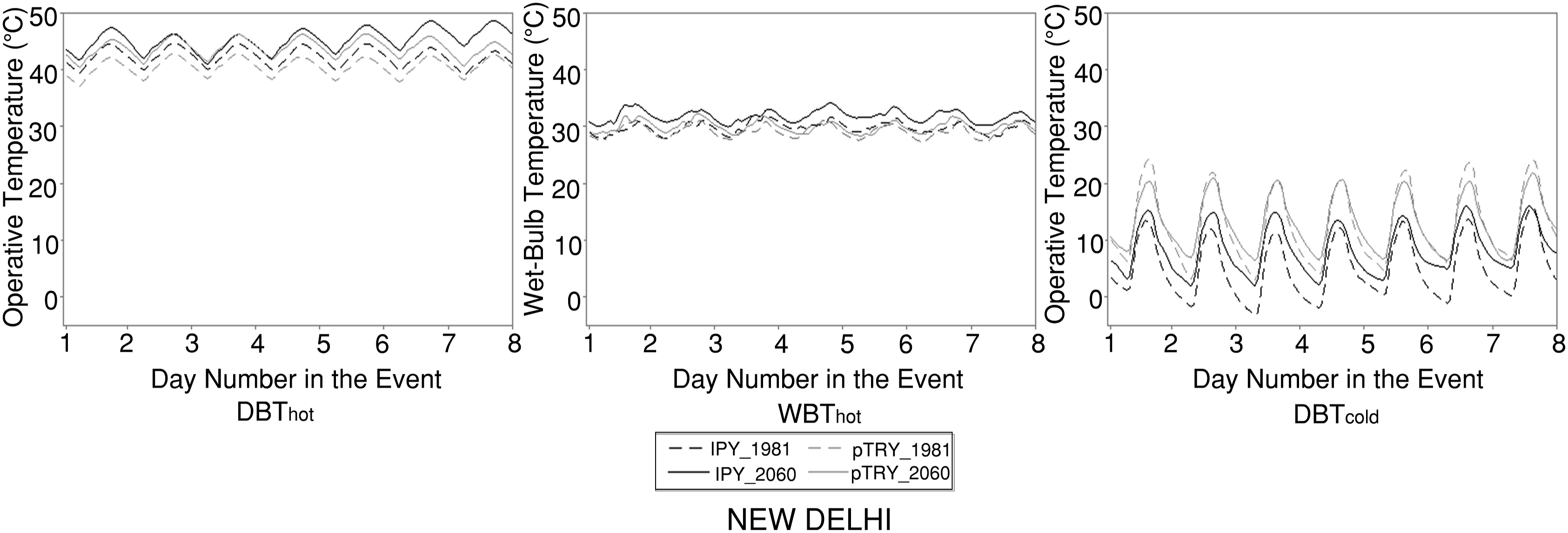

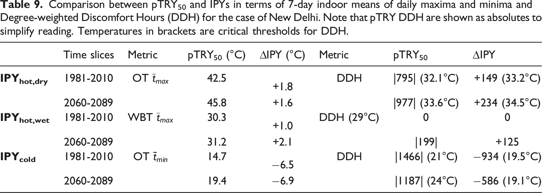
	Time slices	Metric	pTRY50 (°C)	∆IPY (°C)	Metric	pTRY50	∆IPY
IPY hot,dry	1981-2010	OT ${\overline{t}}_{\mathit{max}}$	42.5	+1.8	DDH	|795| (32.1°C)	+149 (33.2°C)
	2060-2089		45.8	+1.6		|977| (33.6°C)	+234 (34.5°C)
IPY hot,wet	1981-2010	WBT ${\overline{t}}_{\mathit{max}}$	30.3	+1.0	DDH (29°C)	0	0
	2060-2089		31.2	+2.1		|199|	+125
IPY cold	1981-2010	OT ${\overline{t}}_{\mathit{min}}$	14.7	−6.5	DDH	|1466| (21°C)	−934 (19.5°C)
	2060-2089		19.4	−6.9		|1187| (24°C)	−586 (19.1°C)

Table 9 shows that the outdoor extreme events present in IPYs translate to consistently more extreme operative indoor temperature values (OT), wet-bulb temperature (WBT) and DDH than the equivalent extreme period in the pTRY₅₀. We observe that indoor peaks are between 1.6 and 1.8°C higher in the IPYs compared to the TRYs. Online Appendix D expands the analysis of these indoor temperatures to other locations, elaborating the impact over different climate types. Figure 9 illustrates the expected spatial changes over time and summarised in Table 10.

Figure 9.

${\overline{\mathit{t}}}_{\mathit{min}\hspace{0.17em}/\hspace{0.17em}\mathit{max}}^{\mathit{i}\mathit{n}}$ indoor temperatures for past (1981-2010) on the left and future (2060-2089) on the right for each extreme type. IPY_hot-dry – (a), (b) represent ${\overline{\mathit{t}}}_{\mathit{max}}$ based dry-bulb, IPY_hot-wet– (c),(d) represent ${\overline{\mathit{t}}}_{\mathit{max}}$ based on wet-bulb, and IPY_cold– (e), (f) represent ${\overline{\mathit{t}}}_{\mathit{min}}$ based on dry-bulb for the extreme event duration. Areas with elevation >1000 m above mean sea level are in white due to lack of good basis data. ‘M’ stands for mean and ‘m’ for median.

Table 10.

Historic and future range for indoor temperatures in each of the three file types covering all 4790 locations are given in square brackets. Means are presented over all 4790 locations for each of the three types of extreme events contained in our IPY files, with standard deviation in brackets. Here, 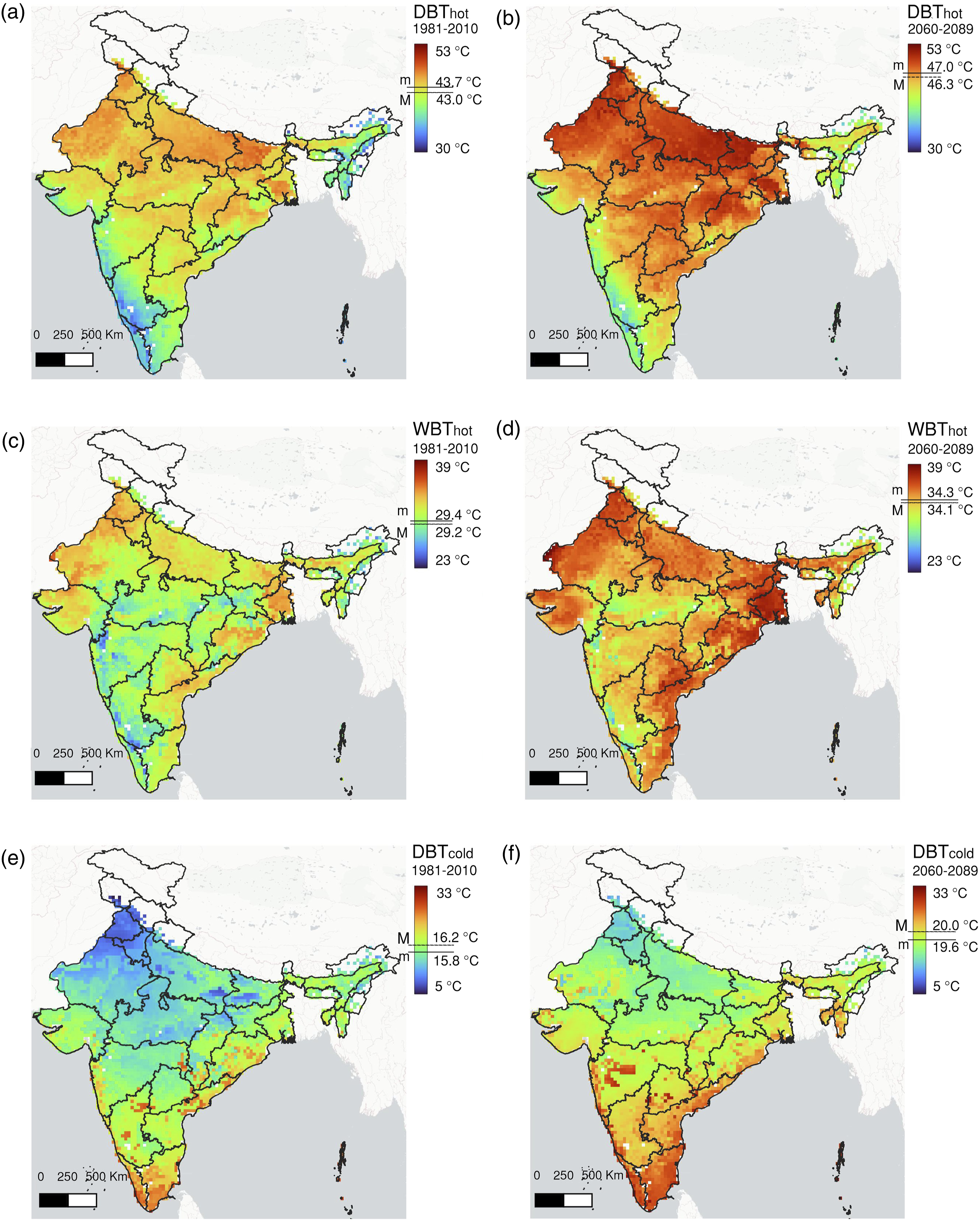$\text{OT}\hspace{0.17em}{\overline{t}}_{\mathit{max}}$ represents the average 7-day daily operative temperature maximum, $\text{WBT}\hspace{0.17em}{\overline{t}}_{\mathit{max}}$ represents the average 7-day daily wet-bulb temperature maximum, and ${\text{OT}\hspace{0.17em}\overline{t}}_{\mathit{min}}$ is the average 7-day daily operative temperature minimum. “[ ]” brackets represents the range over all locations.

File type	Metric (7-day mean)	Historic (1981 – 2010)	Future (2060 – 2089)
IPYhot,dry	OT ${\overline{t}}_{\mathit{max}}$	43.0°C (3.0°C) [31.0°C to 48.3°C]	46.3°C (3.1°C) [34.5°C to 51.6°C]
IPYhot,wet	WBT ${\overline{t}}_{\mathit{max}}$	31.2°C (1.8°C) [21.8°C to 32.8°C]	34.1°C (1.8°C) [23.9°C to 35.2°C]
IPYcold	OT ${\overline{t}}_{\mathit{min}}$	16.2°C (3.9°C) [4.6°C to 30.2°C]	20.0°C (3.8°C) [10°C to 32.5°C]

These uplifts in temperature are complemented by 24% higher DDH in the 2070s compared to the 1990s. The dramatic uplift in DDH above 29°C WBT in the 2070s is noteworthy given that this rise is from a baseline of zero. The neutral temperature underpinning the DDH for both the past (1981-2010) and future (2060-2089) is greater than 18°C, which is the threshold for minimum indoor temperature per WHO housing and health guidelines, ⁵⁵ suggesting no aggregate health-hazardous thermal stress due to IPY_cold, though localised cold-stress will continue in parts of the country as illustrated in Figure 9.

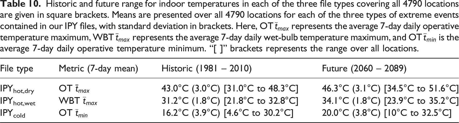
Figure 10 presents the spatially rasterised DDH calculated over each ‘7-Day Extreme Event’. As expected, the future period (2060 - 2089, right side) has higher values of DDH compared to the past (1981 - 2010, left side). These increases in the IPY_hot-dry DDH are accompanied by a commensurate decline in the intensity and number of locations exhibiting cold DDH Figure 10(e) and (f): a decline from 166 locations in the past to only eight in the future.

Figure 10.

Comparison of discomfort degree hours (DDH) for the past (1981-2010) on the left and the future (2060-2089) on the right. IPY-hot (DBT) – (a),(b) represents the summation of DDH over the hot (DBT) extreme event, IPY-hot (WBT) – (c),(d) represents the summation of DDH over the hot (WBT) extreme event, IPY-cold (DBT) – (e),(f) represents the summation of DDH over the cold (DBT) extreme event. In case of IPY-hot (WBT), the critical temperature limit considered is 29°C. The symbols ▲ and ● mark the states of Kerala and Odisha, respectively. ‘M’ stands for mean and ‘m’ for median.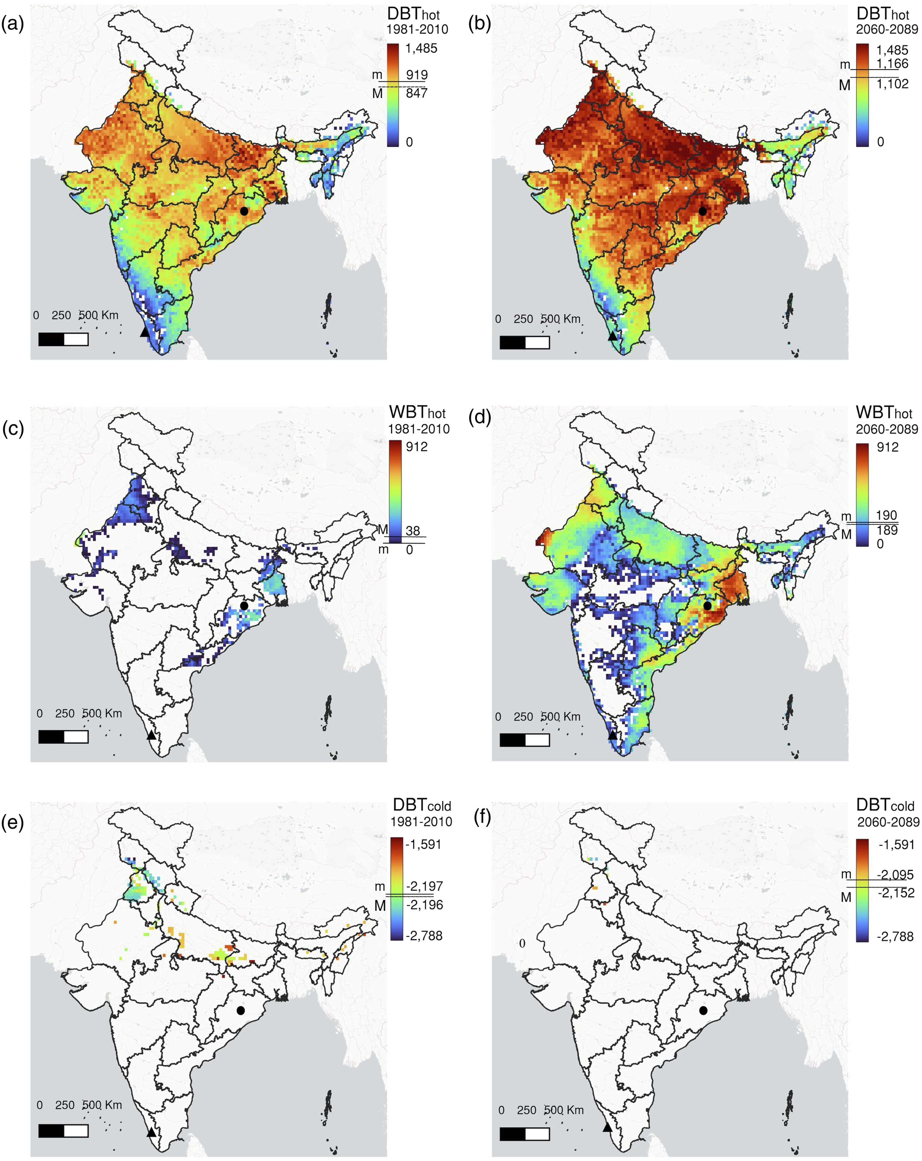

But the most dramatic changes are in the IPY_hot-wet DDH data which show DDH in 605 locations in the 1990s increasing to 3610 locations in the 2070s, Figure 10(c) and (d). Note that the critical threshold temperature of 29°C is considered for IPY_hot-wet as discussed in Section 2.5. Thus, substantial increases in heat stress and consequent increases in latent load are expected in the future compared to today. We pick two states, Odisha and Kerala, on the above maps to illustrate the scale of changes in greater detail, presented below.

The state of Odisha on the east coast (marked with ● in Figures 9 and 10) experiences dramatic changes in both IPY_hot-wet and IPY_hot-dry DDH. Figure 11 (2) shows that in the 1990s, DDH for IPY_hot-dry ∈ [452, 1263] degree hours with neutral temperatures ∈ [30.1, 35] °C over all 258 pixels in this state. This changes to DDH ∈ [574, 1245] degree hours with neutral temperatures ∈ [31.6, 35.4] °C in the future, Figure 11 (2). IPY_hot-wet DDH ∈ [0 – 350] degree hours (83/258 pixels >0 DDH) rising to IPY_hot-wet DDH ∈ [0, 883.2] degree hours (241/258 pixels >0 DDH) as shown in Figure 11 (3).

Figure 11.

Degree Discomfort Hours (DDH) spatial analysis of Kerala and Odisha.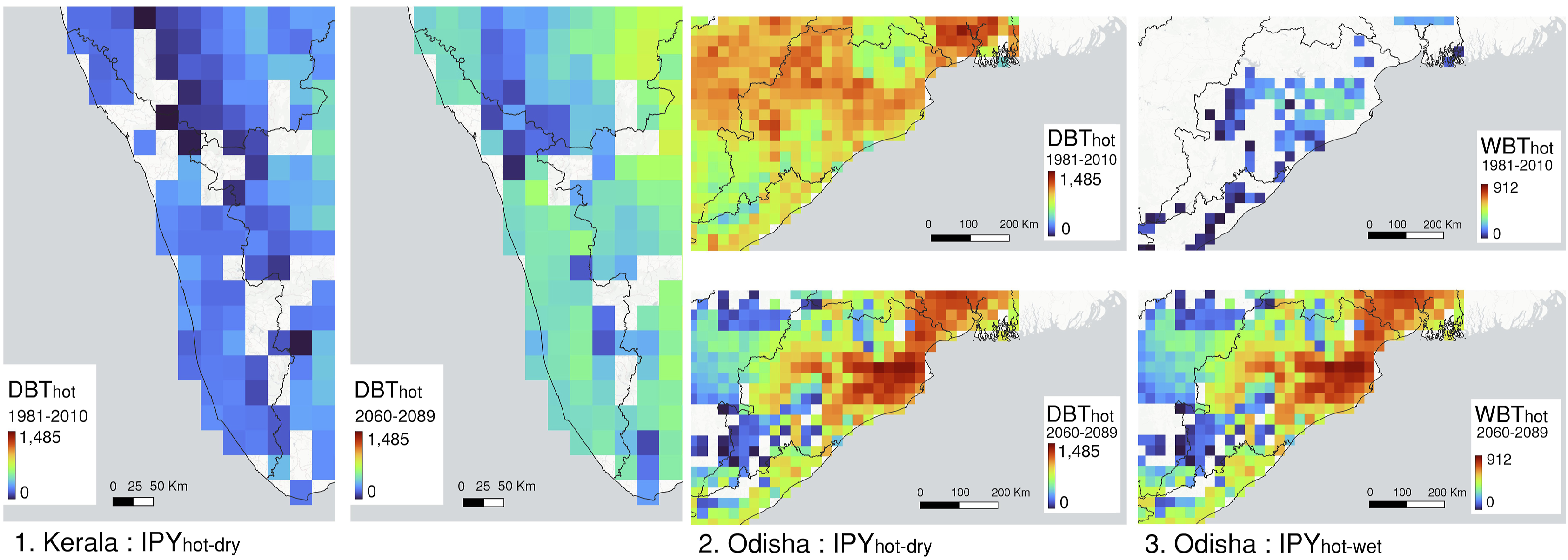

Figure 11 (1) shows Kerala on the southwestern coast (marked with ▲ in Figures 9 and 10), sees substantial changes in IPY_hot-dry DDH. Here, IPY_hot-dry DDH ∈ [0, 348.7] (54/61 pixels >0 DDH) in the 1990s with neutral temperatures ∈ [26.6, 30] °C. However, in the 2070s, DDH ∈ [40, 645] over all 61 data points with neutral temperatures ∈ [28.3, 31.9] °C.

Discussion

Heat and cold stress can have a significant impact on the human body. Implementing measures to mitigate these effects is therefore crucial for safety and well-being. Many studies across different countries have associated extreme temperatures with rising mortality, resulting in the adoption of heat-health warning systems specifically for heat stress based on indices which quantify the effect of meteorological factors (air temperature, relative humidity and global horizontal irradiation) to represent the actual human thermal situation during extreme events.^61,62

Here, we select a sample of indices to measure thermal stress perceived by humans caused by extreme events from those recognised by IMD ⁶³ for discussion. These are, the Heat Wave Magnitude Index (HWMI) defined as “the maximum of all heat wave magnitudes for a given year” and is based on the daily maximum air temperature ⁶⁴ ; Heat Index which is based on a complex iterative procedure but designed to express the combined effect of air temperature and relative humidity as an apparent temperature (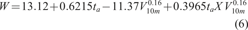 $t_{app}$ )^65,66; and the Wind Chill Index for cold stress which expresses the perceived minimum temperature influenced by wind flow as the wind chill effective minimum temperature (WCTn).^4,67 A Cold Wave is declared when the WCTn deviates from the normal minimum temperature by −5°C to −6°C in regions where the normal minimum temperature exceeds 10°C, and by −4°C to −5°C in other areas. The equation used to calculate the wind chill index is:

$W=13.12+0.6215t_a-11.37V_{10m}^{0.16}+0.3965t_{a}X\hspace{0.17em}{V}_{10m}^{0.16}$

(6)where, W = wind chill index (°C), $t_a$ = air temperature (°C), and V_10m = wind speed at 10m (km/h). The reader is referred to the preceding works for a full definition of each term.

Table 11 illustrates the impact on these indices for New Delhi using both IPYs and pTRYs₅₀, all showing substantial increases in heat stress and decreases in cold stress. The heat wave magnitude index calculated for IPY_hot-dry shows our IPYs produce heatwaves 3°C warmer than the pTRY₅₀. Heat index calculated using IPY_hot-wet suggests significant number of hours beyond the 41°C and 54°C thresholds in the future compared to the past, though IPY-pTRY differences for the latter threshold are not significant. As expected, the wind chill index is calculated using the IPY_cold shows a drop by 4°C and 5°C respectively for past and future in IPYs against the comparator pTRYs₅₀. The possibility of such changes should be cause for concern and prompt the evolution of new strategies to ensure that not only buildings but outdoor environments as well as industrial and agricultural output remain resilient, low-carbon and cost-competitive in the future.

Table 11.

Thermal stress indices for New Delhi computed using IPYs and their corresponding pTRY_50.

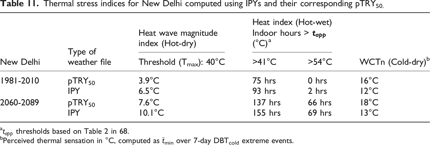
New Delhi	Type of weather file	Heat wave magnitude index (Hot-dry)	Heat index (Hot-wet) Indoor hours > ${\mathit{t}}_{\mathit{a}\mathit{p}\mathit{p}}$ (°C) a		WCTn (Cold-dry) b
		Threshold (Tmax): 40°C	>41°C	>54°C
1981-2010	pTRY50	3.9°C	75 hrs	0 hrs	16°C
	IPY	6.5°C	93 hrs	2 hrs	12°C
2060-2089	pTRY50	7.6°C	137 hrs	66 hrs	18°C
	IPY	10.1°C	155 hrs	69 hrs	13°C

^a $t_{app}$ thresholds based on Table 2 in 68.

^bPerceived thermal sensation in °C, computed as $\overline{t}$ _min over 7-day DBT_cold extreme events.

To evaluate the impact of climate change based on extreme event ( ${\overline{t}}_{\mathit{max}\hspace{0.17em}/\hspace{0.17em}\mathit{min}}$ ) values, the 10^th and 90^th percentile of extreme events for the past (1981 - 2010) are calculated in Table 12. This same threshold is then used to calculate the addition or subtraction in the number of locations in the future dataset. These data lend substance to the significant increases in the occurrence of “hot-wet” type of extreme events compared to “hot-dry” seen in Figure 5. The reduction in the number of locations below 10th percentile threshold ${\overline{t}}_{\mathit{min}}$ from 478 to four indicates the impact of a warming climate, underscoring the impacts shown in Figures 9 and 10.

Table 12.

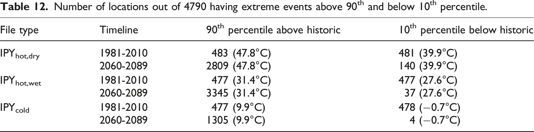
Number of locations out of 4790 having extreme events above 90^th and below 10^th percentile.

File type	Timeline	90th percentile above historic	10th percentile below historic
IPYhot,dry	1981-2010	483 (47.8°C)	481 (39.9°C)
	2060-2089	2809 (47.8°C)	140 (39.9°C)
IPYhot,wet	1981-2010	477 (31.4°C)	477 (27.6°C)
	2060-2089	3345 (31.4°C)	37 (27.6°C)
IPYcold	1981-2010	477 (9.9°C)	478 (−0.7°C)
	2060-2089	1305 (9.9°C)	4 (−0.7°C)

As noted earlier, the PRECIS (RCM) used here under the IPCC “Medium-High” A1B scenario lies somewhere between the newer Reference Concentration Pathways (RCP) 4.5 and RCP 6, both of which assume varying levels of mitigation in their construction and arguably do not represent the most extreme conceivable conditions in the future.^46,47 Thus, the dramatic shifts we demonstrate between the events of the 1990s versus those in the 2070s should give cause for concern to the building design community. While the methods we present can now be applied to other datasets as they improve in fidelity and resolution over time, the data we present can be seen as helping “designing in” climate resilience for a medium to medium-high level of risk.

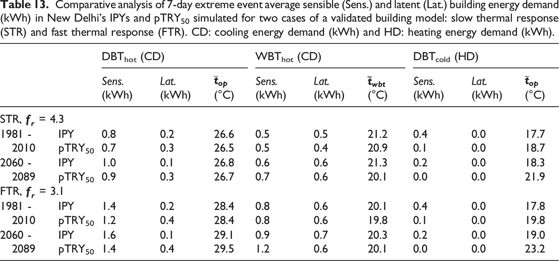
To illustrate these implications for energy demand, the validated building model discussed in Section 2.4 is set to two conditions: Case 1 with slow thermal response (CIBSE response factor, $f_r$ = 4.3 ⁶⁹ ) and Case 2 with fast thermal response ( $f_r$ = 3.1) based on a widely used construction system in India, detailed in Online Appendix E. To extract thermal loads based on outdoor climatic conditions, an ideal air load system is considered having fixed cooling and heating set-points of 25°C and 18°C, respectively. The capacity of the air-conditioner is set to 5.3 kW (1.9 kW conditioning draw), equivalent to a 1.5 ton unit commonly used in Indian homes. This is scheduled to be ‘on’ continuously for simplicity and simulated for New Delhi (Cwa climate), for consistency with the preceding discussion.

Table 13 suggests that the IPY_hot-dry and IPY_cold events produce higher sensible, and the IPY_hot-wet higher latent, thermal demand compared to the corresponding 7-day event contained in the pTRY₅₀. Given that there are instances with equal latent loads in the IPY_hot-wet but with differences in indoor wet-bulb temperatures between IPYs and pTRYs, provides further validity to our approach of developing a variety of localised extreme week signatures, and a step change in the current state of the art.

Table 13.

Comparative analysis of 7-day extreme event average sensible (Sens.) and latent (Lat.) building energy demand (kWh) in New Delhi’s IPYs and pTRY₅₀ simulated for two cases of a validated building model: slow thermal response (STR) and fast thermal response (FTR). CD: cooling energy demand (kWh) and HD: heating energy demand (kWh).

		DBThot (CD)			WBThot (CD)			DBTcold (HD)
		Sens. (kWh)	Lat. (kWh)	${\overline{\mathit{t}}}_{\mathit{o}\mathit{p}}$ (°C)	Sens. (kWh)	Lat. (kWh)	${\overline{\mathit{t}}}_{\mathit{w}\mathit{b}\mathit{t}}$ (°C)	Sens. (kWh)	Lat. (kWh)	${\overline{\mathit{t}}}_{\mathit{o}\mathit{p}}$ (°C)
STR, ${\mathit{f}}_{\mathit{r}}$ = 4.3
1981 - 2010	IPY	0.8	0.2	26.6	0.5	0.5	21.2	0.4	0.0	17.7
	pTRY50	0.7	0.3	26.5	0.5	0.4	20.9	0.1	0.0	18.7
2060 - 2089	IPY	1.0	0.1	26.8	0.6	0.6	21.3	0.2	0.0	18.3
	pTRY50	0.9	0.3	26.7	0.7	0.6	20.1	0.0	0.0	21.9
FTR, ${\mathit{f}}_{\mathit{r}}$ = 3.1
1981 - 2010	IPY	1.4	0.2	28.4	0.8	0.6	20.1	0.4	0.0	17.8
	pTRY50	1.2	0.4	28.4	0.8	0.6	19.8	0.1	0.0	19.8
2060 - 2089	IPY	1.6	0.1	29.1	0.9	0.7	20.3	0.2	0.0	19.0
	pTRY50	1.4	0.4	29.5	1.2	0.6	20.1	0.0	0.0	23.2

Conclusion

The climate is changing and extreme weather phenomena are expected to become more frequent and intense. Yet, a consistent definition of such extreme events does not yet exist, with many countries choosing local definitions based on absolute, potentially arbitrary, temperature thresholds. Some of these definitions, as is the case with India, can have overlapping elements or other inconsistencies with the potential for confusion. That humidity is not explicitly accounted for in these definitions exposes designers, policy makers and other professionals to further risk given that the weather in many locations is expected not merely get warmer but also wetter and more humid as the climate changes.

Here, we provide a locally meaningful yet globally consistent definition of such extreme events with the primary aim of being used to design climate resilient buildings, but with potentially much wider application in the built and natural systems. We show how this definition can be used to extract a variety of events comprising hot-dry, hot-wet and cold-dry extreme events and that the ideal length of such events is 7-days. These are extracted for the case of India at a 25 km × 25 km spatial resolution using carefully calibrated computer-generated weather data. This produced six extreme event files (3 event types × 2 time slices, current and future), termed Indian Peak Years (IPY) for simplicity. Over 4790 locations, this translates to 28,740 files in total. It is noteworthy that no extreme event data for India exist at present.

We subject these files to a series of tests including validation against known extremes (mean bias error against all known dry-bulb hot extremes of +0.2°C (σ = 2.4°C) over a 100-year period), internal consistency (mean deviation of 4.5°C, σ = 4.9°C, compared to the equivalent extreme period in a typical year) and temporal consistency (86% of events are within ±30 days of a baseline comparator); all suggesting a high degree of reliability. Consistency information is coded within the files to aid user judgement.

Our data use the IPCC scenario A1B (rapid economic growth, globalisation, rapid introduction of new and more efficient technologies, and a balance between fossil and renewable energy sources), lying somewhere between the recent RCP 4.5 and 6.0 pathways. This medium / medium-high emission scenario is therefore conservative compared to high emission scenarios. Even so, we see the 50°C threshold breached in several parts of the country, with the highest one-hour temperature in an IPY_hot-dry for the future (2060-2089) is 54.9°C. Similarly, the IPY_hot-wet event’s maximum and IPY_cold event’s minimum one-hour value for the future period is 36.2°C (WBT and −2.8°C (DBT), respectively. Of these, it is the WBT data that are the most worrying given that the theoretical upper limit for 6 hour exposure is 35°C, and the regular breaches of the potential real limit of around 31°C observed in our results.

These data presage significant impacts on buildings, further raising internal temperatures, as we have shown. We also briefly highlight how strategies such as thermal mass can help blunt some of these effects. We hope that other researchers will use our data to explore these impacts in greater detail, resulting in more climate-resilient buildings and infrastructure.

Finally, the generated IPY files have been placed in a free-to-use publicly repository (see acknowledgements). Though the proposed method identifies heat waves and cold snaps lasting for 7 days, it can be utilised to generate extreme weather files for longer durations, such as 10 or 12 days. Similarly, the selection percentile for hot extremes set to 99.9^th and cold extremes set to 0.1^th can be altered to meet user needs.

The presented methods and weather files are hence anticipated to be highly beneficial not only to building professionals who use modelling or simulation techniques, but also more widely to entities engaged in assessing the potential impacts of climate change in a spectrum of sectors and by policy makers at local to national level.

Supplemental Material

Supplemental Material - Accurate representations of locally meaningful future extreme weather events and the implications for India

Supplemental Material for Accurate representations of locally meaningful future extreme weather events and the implications for India by Shweta Lall, Oliver Hatfield, David Coley Isha Rathore, Rajasekar Elangovan, Dhyan Singh Arya, Hangyeol Park and Sukumar Natarajan in Building Services Engineering Research & Technology.