Sage Journals: Discover world-class research

Abstract

This study evaluates the thermal performance of geothermal borehole heat exchangers (BHEs) in various Canadian locations during winter, focusing on soil freezing effects. Using a computational fluid dynamics approach, it examines how soil porosity and thermal conductivity influence BHEs’ thermal performance. Ninety case studies across nine Canadian zones assessed these effects under winter conditions. The RNG k-ɛ turbulent model tracked fluid flow, and the solidification model monitored ice formation. Soil temperature fluctuations along the ground depth were incorporated using user-defined function codes. Coefficients of performance (COP) were calculated for heat pump thermal performance. Results showed substantial soil freezing around the borehole in Saskatchewan and Manitoba. The BHE systems in Alberta and Manitoba had the highest thermal resistance, while those in Saskatchewan and Prince Edward Island had the lowest. Increasing soil porosity from 0.4 to 0.55 and decreasing thermal conductivity from 2.0 to 1.385 W/mK led to up to 40% and 58% increases in ice formation, respectively. The COP of the heat pump in British Columbia was maximized, reflecting the peak temperature of the outlet fluid from the BHE. By incorporating site-specific climatic data and addressing gaps in existing standards, this research enhances geothermal system guidelines with practical design recommendations.

Practical application

This study provides built environment professionals with valuable insights into optimizing geothermal borehole heat exchangers (BHEs) for cold climates, particularly across various Canadian regions. By incorporating site-specific soil and climatic data, the research identifies key factors, such as soil porosity and thermal conductivity, that influence system performance. The findings will guide professionals in designing more efficient BHE systems, reducing ice formation, and improving heat pump efficiency. These design enhancements ensure that geothermal systems operate effectively in cold climates, contributing to sustainable heating solutions in residential and commercial buildings.

Keywords

Borehole heat exchanger computational fluid dynamics soil freezing thermal resistance ground temperature profile coefficient of performance

Introduction

Overview

Geothermal energy, sourced from the earth’s depths, is a dependable and eco-friendly source of energy suitable for heating and cooling purposes.¹ Ground source heat pumps (GSHPs) can provide energy efficiency three to five times higher than traditional combustion-based electrical heaters.² In different weather conditions, GSHPs can serve in cooling or heating roles.³ In winter, GSHPs convey geothermal heat to building heating systems, while in summer, they collect heat from buildings for cooling purposes.⁴ A GSHP system consists of three main components: a borehole heat exchanger (BHE) or ground loop, a heat pump, and a heat transmission system.⁵ Based on Figure 1, the heat from the ground is initially transferred to the borehole and, subsequently, to the working fluid within the tube. This extracted heat is transported to the heat pump via the circulating fluid. Finally, the heat pump channels the geothermal energy to the water-based heating systems.⁶ Using BHE for geothermal energy extraction offers advantages, including minimal environmental impact, high durability, and low-risk drilling operations.⁷ Practices in Canada, the United States, mainland Europe, and Japan typically involve backfilling the borehole with grout.

Figure 1.

(a) GSHP system configuration for heating purposes and the (b) geometry for borehole heat exchanger.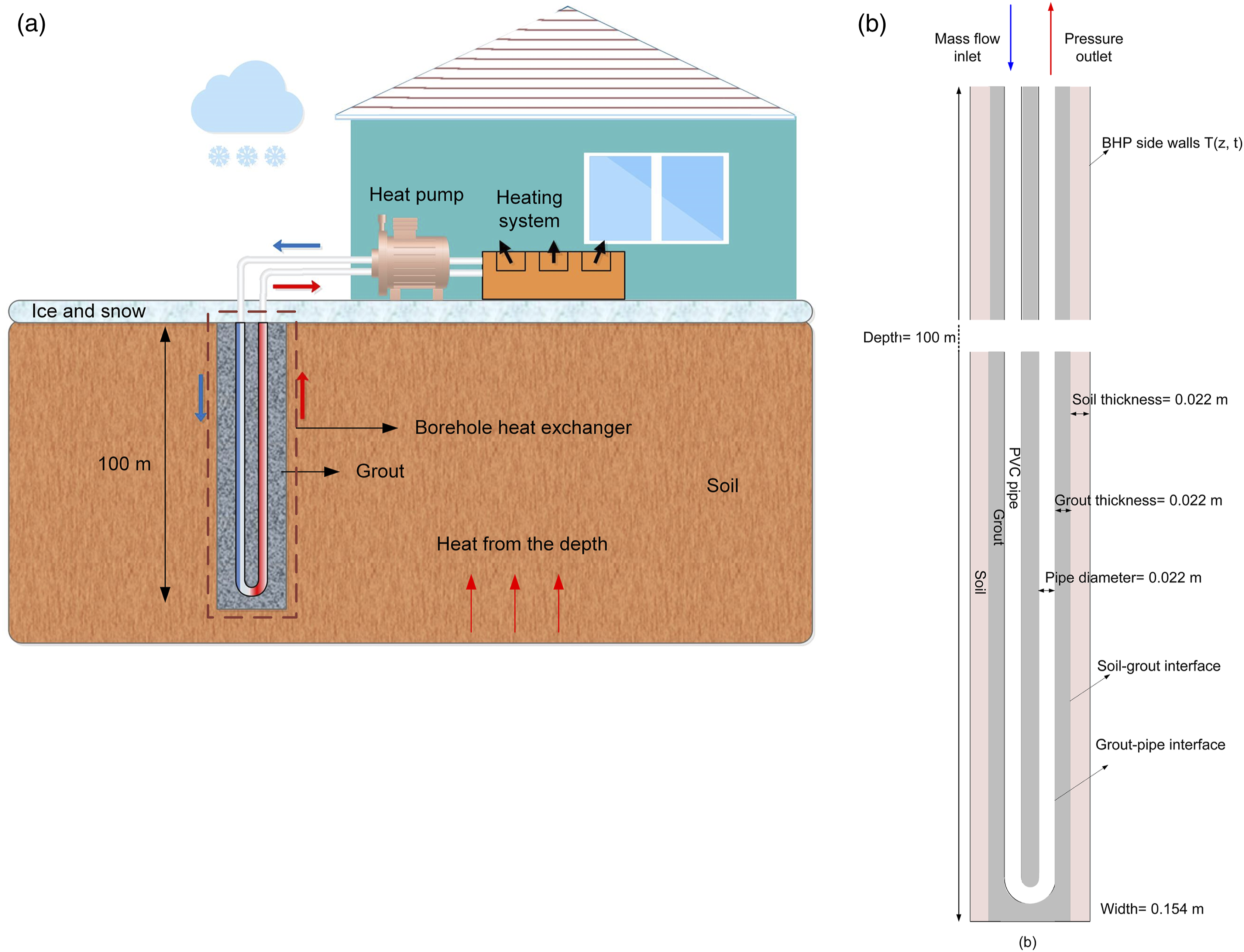

Effective parameters in GHSP performance

As reported in the literature, the thermal efficiency of the borehole is influenced by the fluid flow rate, pipe geometry, pipe material, and thermal properties of the grout.^8,9 Findings suggested that under specific geometry and conditions, the thermal efficiency of the borehole improves with higher thermal conductivity of the grout or fluid-conducting pipe.¹⁰ In addition, the thermal conductivity of the soil surrounding a BHE is a critical factor influencing heat transfer and overall GSHP thermal performance.^11,12

Numerous studies in the literature have focused on optimizing the design parameters of BHEs¹³ using combined response surface methodology and multi-objective genetic algorithm,¹⁴ COMSOL Multiphysics software,¹⁵ ANSYS Fluent software,¹⁶ and 1D computational approach.¹⁷ Using a developed transient heat transfer model, Kerme et al.¹⁸ suggested that optimizing the design parameters, such as increasing borehole depth, adjusting shank spacing, and selecting appropriate working fluids, could significantly enhance the thermal performance of borehole heat exchangers.

The thermal behavior of the BHE influences the heat pump’s coefficient of performance (COP), which is defined based on the heat pump’s performance relative to the heating or cooling objectives of the GSHP systems. A high COP of the heat pump serves as an indicator of the satisfactory thermal performance of the BHE.¹⁹ However, the COP of the heat pump can be affected by various conditions, such as evaporation and condensation temperatures.²⁰ Despite this, literature reports on the impacts of these variations usually focus either on the heat pump’s inlet fluid temperature or BHE’s outlet fluid temperature.^21,22 Also, in extremely cold weather conditions, the COP of the GSHP tends to decrease because of the larger temperature differential between the ground source and the destination.²³

Application of GSHP in cold climate zones

The literature has shed light on the impact of coil freezing in air-source heat pumps due to the presence of moisture and the harsh weather conditions in Canada.²⁴ The occurrence of ice and snow in cold climates has been acknowledged as an important factor influencing GSHP thermal efficiency. In a thermo-economic-environmental study, Nikitin et al.²³ discussed the challenges of heat pump performance in cold climate zones, particularly areas heavily blanketed by ice and snow. Also, they provided comparative data on the optimal performance of GSHPs at ten different geographical locations in Russia during winter. Their work highlighted the impact of borehole sizing and heat pump capacity on total costs and energy efficiency. Thus, Canada and Russia, which represent some of the coldest residential climate zones, can be considered critical regions for GSHP installations. Using CFD and experimental analysis, Flaga-Maryanczyk et al.²⁴ evaluated a ground source heat exchanger system’s performance in a cold climate for a passive house ventilation system. In February, the coldest month, the GSHE provided an average of 24% of the heat required for heating the ventilation air, demonstrating significant energy savings and efficiency. Table 1 summarizes the previous literature studies focusing on the GSHP systems’ thermal performance under soil freezing in cold regions.

Table 1.

Previous studies on the thermal performance of GSHP system under soil freezing in cold regions.

Ref	Effective factors on thermal performance	Numerical methodology	Geographical location
²⁵	Ground thermal conductivity, saturated sand ring radius, borehole configuration	1-D radial heat transfer model development	Montréal, Québec
²⁶	Thermal conductivity of soil, soil saturated level, borehole configuration, insulation length	Dual continuum approach using OpenGeoSys software	Taucha, Germany
²⁷	Grout mate freezing interval, temperature distributional properties, specific heat capacity, thermal conductivity, and porosity	A finite element model using the FEFLOW software	Germany
²⁸	Moisture content, radiant heat lamp	In-house software was utilized for temperature data collection	Ferrara, Italy
²⁹	Soil freezing, groundwater flow, and load ratio	COMSOL multiphysics 5.3a	Northeast China
³⁰	Soil temperature, buried pipe depth, thermal conductivity and specific heat capacity, inlet and outlet water temperatures, and soil density	Fractal theory using TRNSYS	Harbin, China
³¹	Inlet water-glycol temperatures	RC model development	Shanghai, China
³²	Heat carrier fluid, soil type and moisture, and borehole geometrical parameters	Finite element model considering freeze-thaw cycles	Venice (northern Italy)
³³	The inlet temperature of the fluid, soil thermal properties, antifreeze properties	An analytical model to predict the behavior of the thermosyphon system in freezing soil	Not specified a particular geographic location
³⁴	Water content and soil type	Two-dimensional heat transfer model including phase change	Cold regions, not specified
This work	Soil freezing, porosity, thermal conductivity, ice formation, thermal resistance, and COP of heat pump assessing the efficiency of BHE systems under cold and extreme cold conditions	CFD simulations with solidification models and site-specific climatic data	Nine locations across Canada

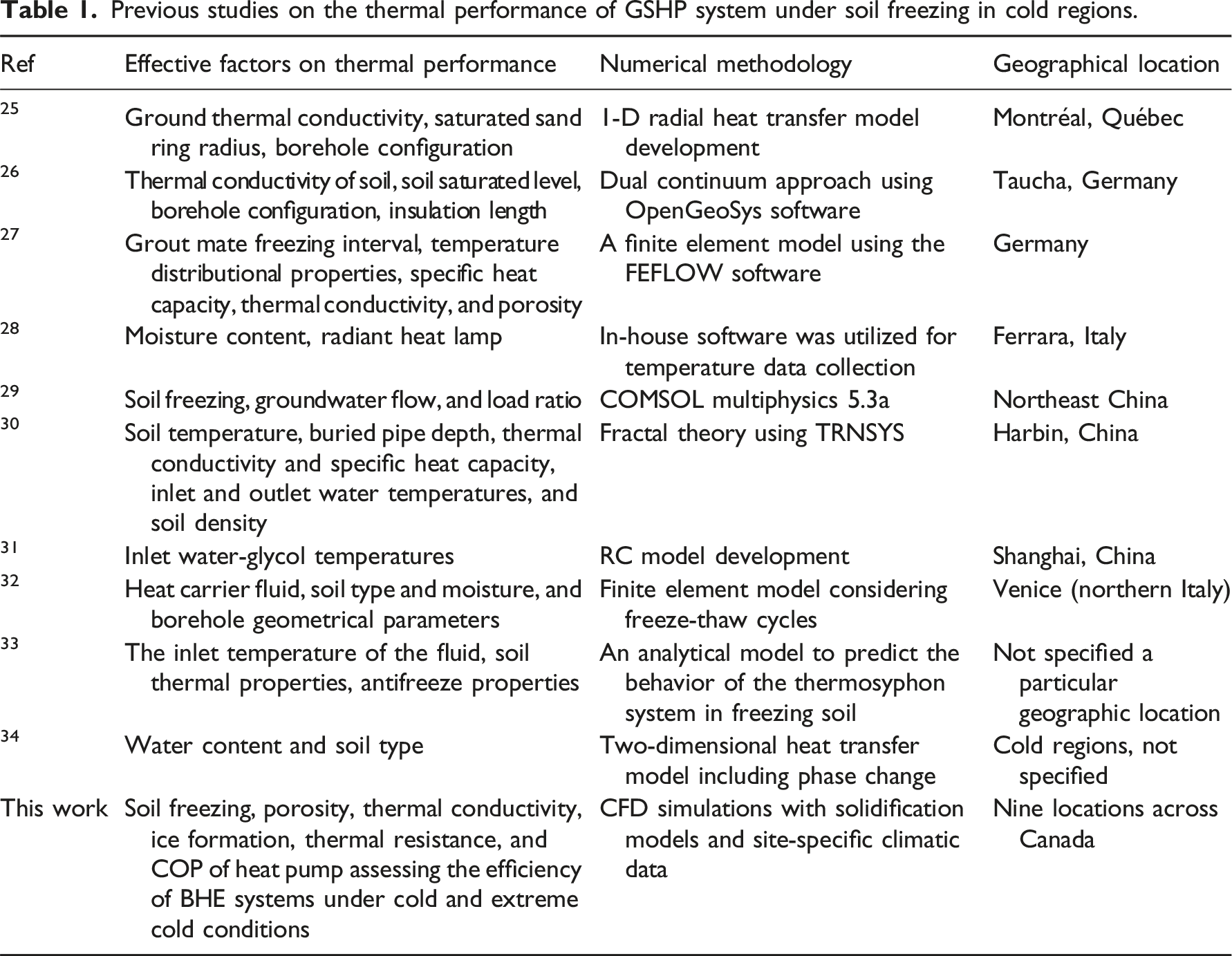
Although many studies have examined the effects of soil freezing and icing around borehole heat exchangers, taking into account the properties of soil, grout, and antifreeze, there remains a lack of comparative research that explores the impact of soil freezing on the performance of borehole heat exchangers across various Canadian locations using the latest soil property data and weather conditions on these locations. Unlike existing studies, this work introduces a comparative framework across nine distinct Canadian locations, integrating CFD simulations to evaluate how site-specific soil porosity and thermal conductivity influence ice formation and thermal resistance. This approach surpasses previous investigations in terms of:

1. Geographical scope and specificity: Prior research often focuses on isolated locations such as Germany or China. The present work uniquely assesses regional variations across Canada, covering diverse soil and climatic profiles. The inclusion of these dynamics into site-specific guidelines establishes a novel framework for assessing the efficiency of BHE systems under extreme cold conditions.

2. Integration of solidification models: Previous studies do not comprehensively incorporate ice formation’s role in BHE performance. This work applied the solidification model to directly analyze ice formation, coupled with detailed soil temperature profiles, bridges this critical gap.

3. Enhanced Practical Guidelines: While earlier research provided theoretical insights, this study delivers practical design recommendations tailored for Canadian climates, addressing specific gaps in standards like ANSI/CSA/IGSHPA C448 Series-16³⁵ by focusing on the effects of soil freezing and ice formation on BHE performance. Hence,

• Advanced CFD simulations provided detailed insights into thermal interactions.

• Site-specific climatic data and seasonal variations were included to offer tailored recommendations for different Canadian locations.

• Practical design guidelines based on empirical data were provided to optimize parameters such as soil porosity and thermal conductivity.

These contributions ensure that geothermal systems designed with these enhancements will be more efficient and reliable in cold climates. Hence, this study concentrates on CFD simulation of the BHE, to identify dependencies of ice formation and thermal resistance on soil porosity and thermal conductivity during winter across various geographical zones in Canada. Therefore, the primary contribution of this work lies in applying the specific soil properties of each geographical location, while considering local weather conditions and temperature variations through the ground depth at these locations. In addition, this work presents results on the thermal resistance of the BHE to identify the most thermally efficient locations for BHE installation in Canada during winter. Also, the COP of the heat pump, which will be added to the BHE, is calculated based on the final results of the BHE’s thermal performance. These insights provide crucial guidance for policymakers and geothermal system designers. This data will assist them in selecting the most suitable installation locations, taking into account thermal performance considerations for building applications.

Problem definition and boundary conditions

Typically, the depth of the BHE ranges from 45 m to 75 m for residential uses and exceeds 150 m for larger industrial applications.³⁶ Additionally, other sources note that the pipes are installed within wells ranging from 50 m to 150 m in depth.^37,38 Therefore, 100 m is a reasonable depth for the simulation in the current study. Moreover, a borehole diameter of 0.154 m is considered appropriate for residential applications.^15,29,36,39 The maximum radius that a borehole heat exchanger (BHE) can affect the surrounding soil is typically between 8 and 10 m. On the other hand, for deep BHEs (e.g., more than 50 m in depth), the influence of surface climate at depth becomes negligible. However, in this work, the primary focus is on the near-field effect, particularly the ice formation around the borehole. Therefore, as shown in Figure 1, the BHE features a U-shaped tube with a 100 m depth⁴⁰ embedded in grout and porous soil. The inlet and outlet diameters of the tube measure 25 mm.⁴¹ A fluid mixture of water and glycol (an anti-freeze agent) is channeled from the left side of the U-shaped pipe with a certain temperature and exits from the right side. The top walls, representing soil, are held at ambient temperature. Sidewalls of the borehole account for different temperature profiles throughout the ground depth defined in equation (17). The boundary conditions between solid-solid zones (soil-grout and grout-soil) and solid-fluid zones (grout-tube) are all defined as thermal interfaces. No adiabatic walls are specified, ensuring that heat transfer occurs naturally between the different regions. This approach allows the model to accurately capture the thermal interactions between materials in contact. For the snow and ambient environment, it is assumed that the ground surface temperature is equal to the ambient temperature. This assumption is valid under steady-state conditions where the surface is in thermal equilibrium with the surrounding air and there are no significant external heat fluxes, such as solar radiation or melting effects. Table 2 presents the boundary conditions and their corresponding values.

Table 2.

Boundary condition values applied in the present study.

Boundary condition (type)	Value
Pipe inlet (mass flow inlet)	0.72 kg/s^42,43
Pipe inlet (temperature)	263 K⁴⁴
Pipe inlet (molar composition)	60% water, 40% ethylene glycol⁴⁵
Pipe outlet (pressure outlet)	0 Pa gauge pressure
Soil 0–100 m (wall)	UDF code for the temperature profile T (t, z)
Soil-grout (interface)	-
Tube-grout (interface)	-
Ground surface (wall)	Ambient temperature (K)

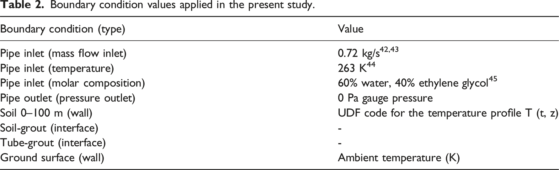
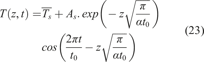
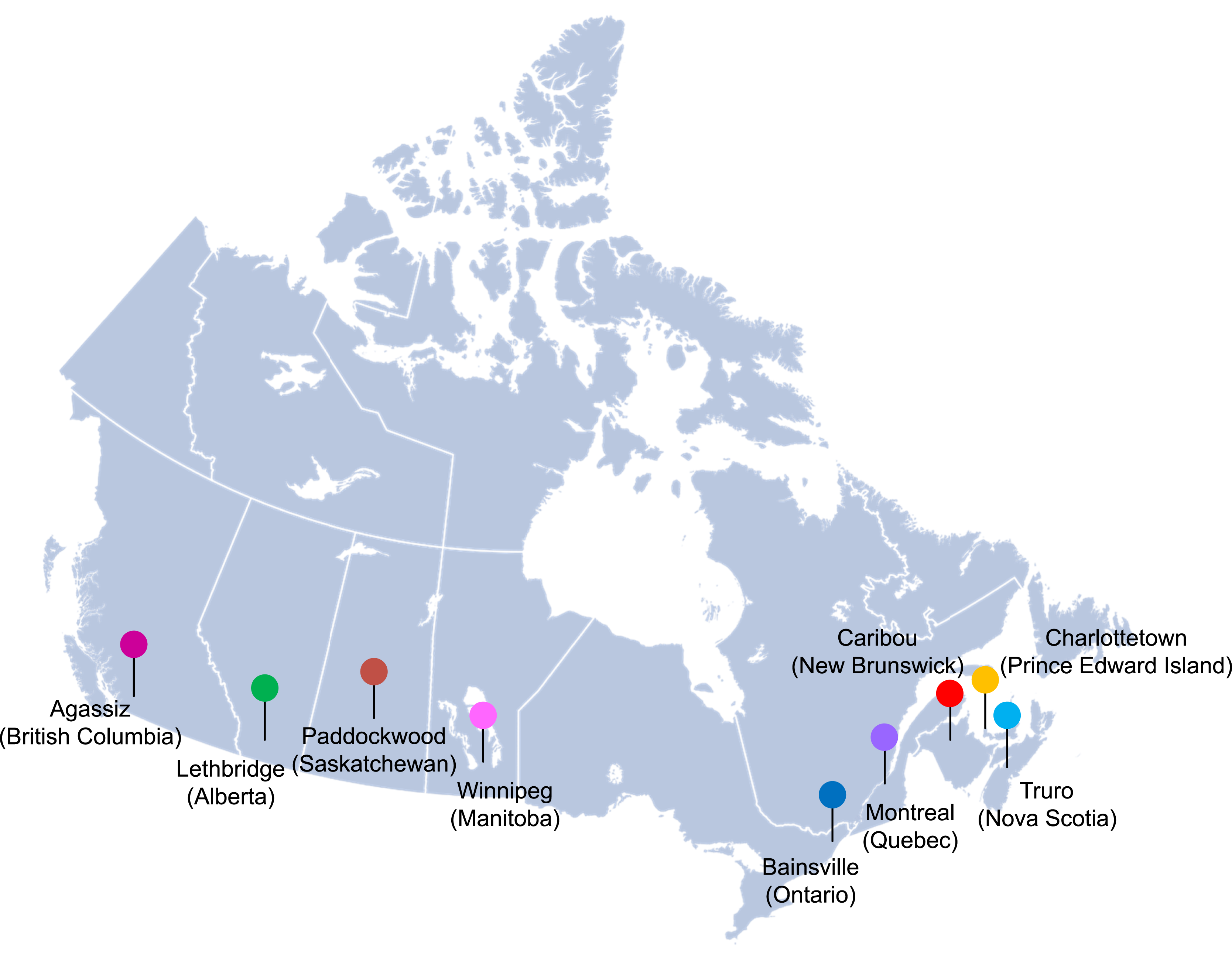
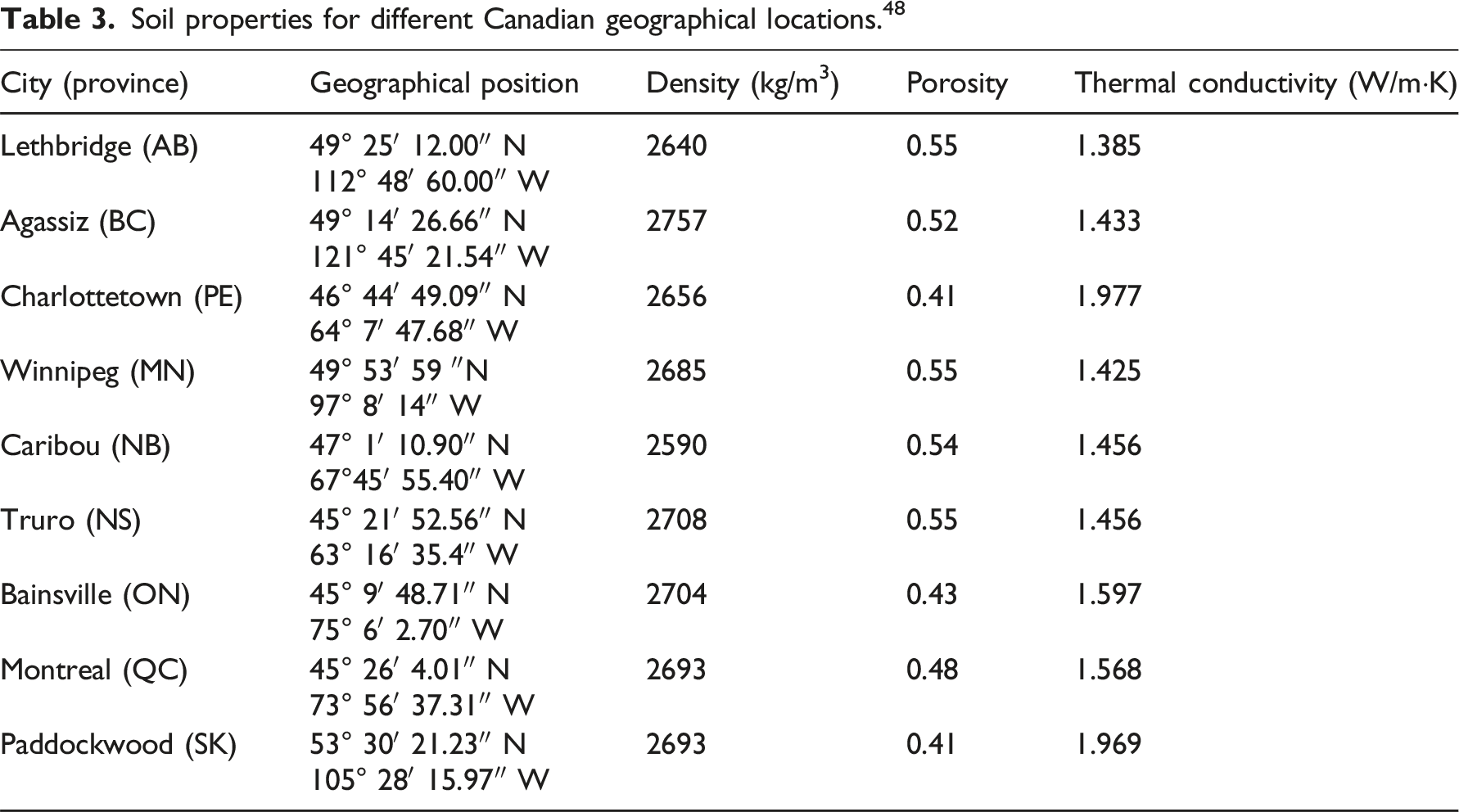
Existing literature establishes that the soil temperature is contingent on ground depth,⁴⁶ with variations differing across locations. In this research, the temperature profile for each city up to the depth of 100 m using equation (17), which is derived from the temperature profile function related to depth in Canada.⁴⁷ Figure 2 shows the nine selected geographical zones in Canada in this study. Table 3 lists the soil properties and temperature data based on geographical locations within Canada. 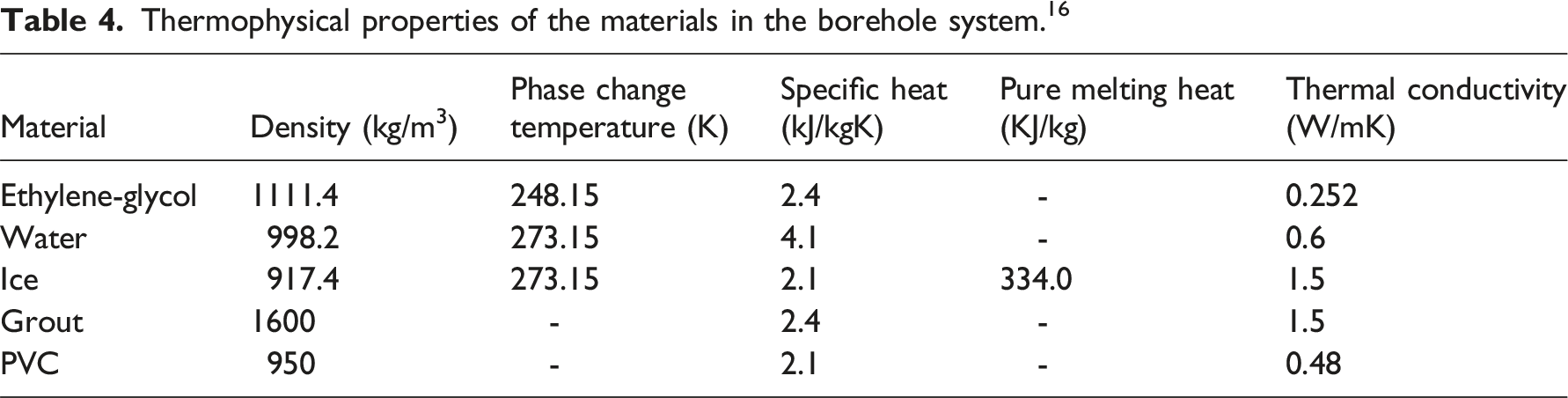The soil properties, such as density, porosity, and thermal conductivity, are derived from the research conducted by Tarnawski et al.⁴⁸ for nine distinct locations in Canada. It should be noted that thermal conductivity data is used for saturated soil. Soil temperatures at the surface are determined based on the average winter temperature (Dec 2021 through Feb 2022) from nine different locations, as sourced from the literature.^49–57 In addition, the thermophysical properties of the materials used in the simulations are summarized in Table 4.

Figure 2.

Selected locations in Canada in this study.

Table 3.

Soil properties for different Canadian geographical locations.⁴⁸

City (province)	Geographical position	Density (kg/m³)	Porosity	Thermal conductivity (W/m·K)
Lethbridge (AB)	49° 25′ 12.00″ N	2640	0.55	1.385
Lethbridge (AB)	112° 48′ 60.00″ W	2640	0.55	1.385
Agassiz (BC)	49° 14′ 26.66″ N	2757	0.52	1.433
Agassiz (BC)	121° 45′ 21.54″ W	2757	0.52	1.433
Charlottetown (PE)	46° 44′ 49.09″ N	2656	0.41	1.977
Charlottetown (PE)	64° 7′ 47.68″ W	2656	0.41	1.977
Winnipeg (MN)	49° 53′ 59 ″N	2685	0.55	1.425
Winnipeg (MN)	97° 8′ 14″ W	2685	0.55	1.425
Caribou (NB)	47° 1′ 10.90″ N	2590	0.54	1.456
Caribou (NB)	67°45′ 55.40″ W	2590	0.54	1.456
Truro (NS)	45° 21′ 52.56″ N	2708	0.55	1.456
Truro (NS)	63° 16′ 35.4″ W	2708	0.55	1.456
Bainsville (ON)	45° 9′ 48.71″ N	2704	0.43	1.597
Bainsville (ON)	75° 6′ 2.70″ W	2704	0.43	1.597
Montreal (QC)	45° 26′ 4.01″ N	2693	0.48	1.568
Montreal (QC)	73° 56′ 37.31″ W	2693	0.48	1.568
Paddockwood (SK)	53° 30′ 21.23″ N	2693	0.41	1.969
Paddockwood (SK)	105° 28′ 15.97″ W	2693	0.41	1.969

Table 4.

Thermophysical properties of the materials in the borehole system.¹⁶

Material	Density (kg/m³)	Phase change temperature (K)	Specific heat (kJ/kgK)	Pure melting heat (KJ/kg)	Thermal conductivity (W/mK)
Ethylene-glycol	1111.4	248.15	2.4	-	0.252
Water	998.2	273.15	4.1	-	0.6
Ice	917.4	273.15	2.1	334.0	1.5
Grout	1600	-	2.4	-	1.5
PVC	950	-	2.1	-	0.48

Numerical approach

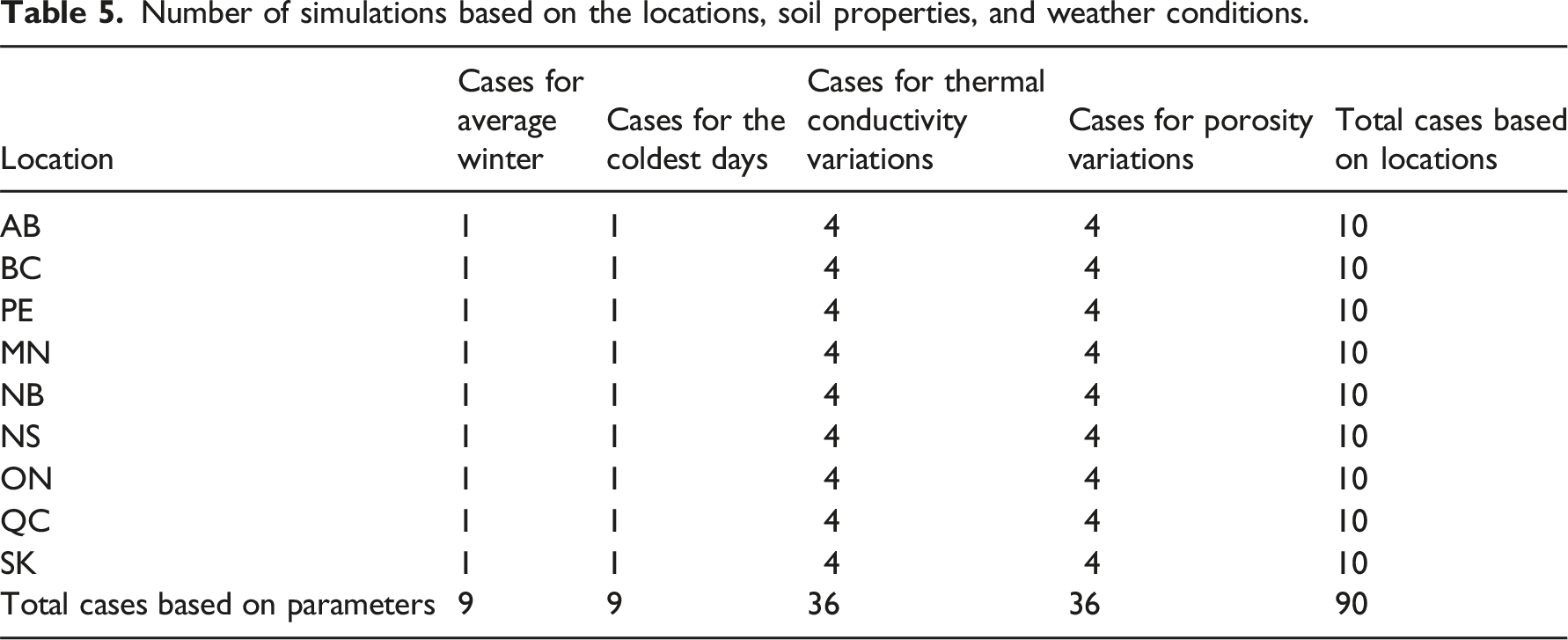
As outlined in Figure 3, this study is divided into three primary stages: pre-processing, processing, and post-processing. The pre-processing stage encompasses the creation of the geometry of the borehole system, meshing, and defining boundary conditions, all undertaken in GAMBIT 2.4.6 software. During the processing stage in ANSYS FLUENT, energy, and k-ɛ realizable turbulent models for the fluid within the U-pipe were activated. In addition, the solidification model was used to monitor ice formation in the soil. The soil, grout, working fluid, and pipe properties were incorporated into the material properties section. Grout was identified as a solid medium. The saturated soil medium was defined as a porous separate zone, including two sections, solid and fluid (water), with different porosities based on the soil type and geographical location. As shown in Table 5, with varying parameters such as porosity, thermal conductivity, and weather conditions in mind, 90 simulations were implemented in ANSYS Fluent software. In the post-processing stage, the data and contours related to ice formation, temperature, and COP are provided.

Figure 3.

Sequence of steps in the CFD simulation of the borehole heat exchanger system.

Table 5.

Number of simulations based on the locations, soil properties, and weather conditions.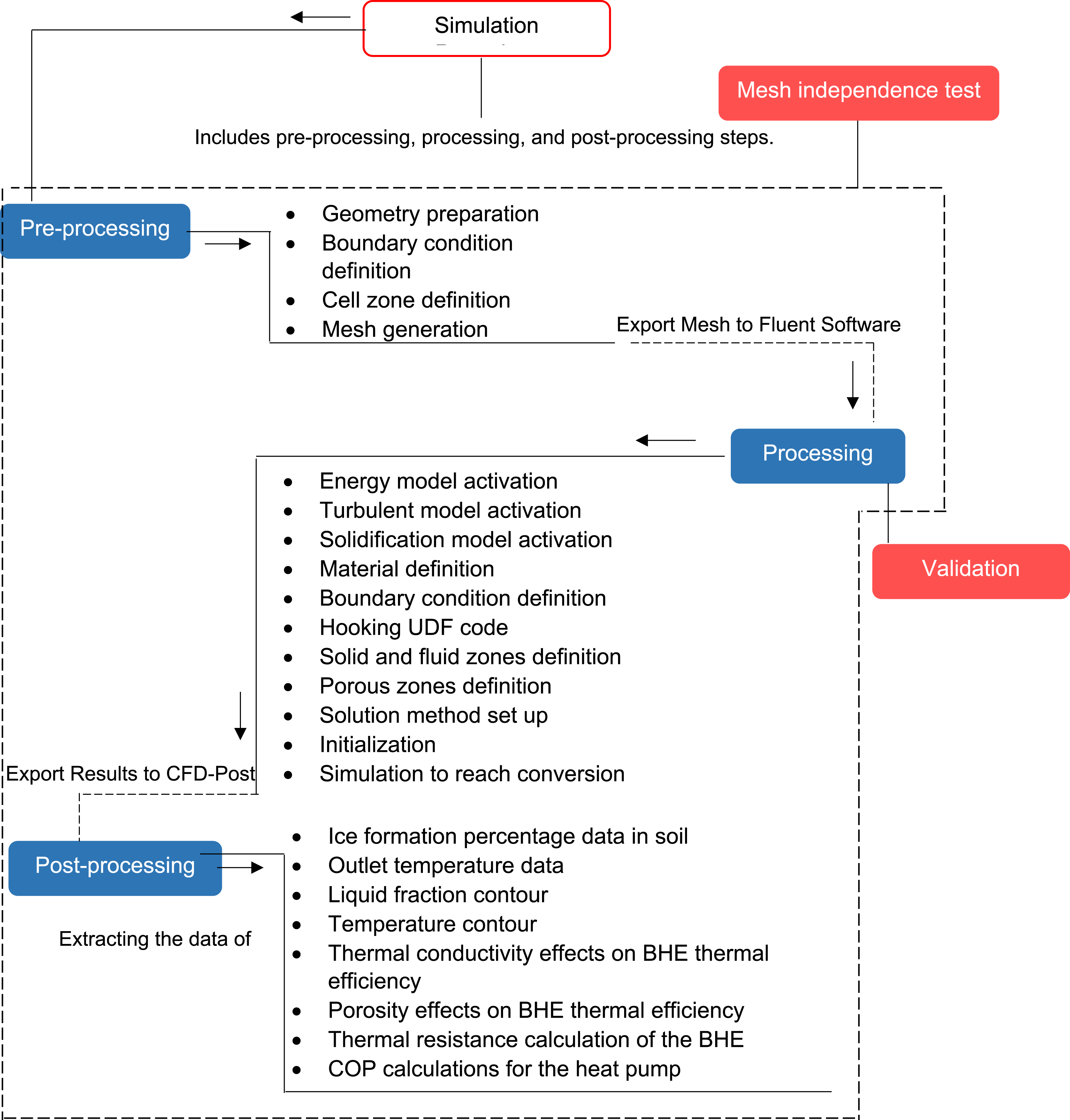

Location	Cases for average winter	Cases for the coldest days	Cases for thermal conductivity variations	Cases for porosity variations	Total cases based on locations
AB	1	1	4	4	10
BC	1	1	4	4	10
PE	1	1	4	4	10
MN	1	1	4	4	10
NB	1	1	4	4	10
NS	1	1	4	4	10
ON	1	1	4	4	10
QC	1	1	4	4	10
SK	1	1	4	4	10
Total cases based on parameters	9	9	36	36	90

Governing equations

The steady-state assumption is well-justified in these simulations, as they represent post-equilibrium conditions where phase changes, such as water freezing to ice, have fully stabilized. Each simulation is conducted for a specific day of the year, with the time component referring solely to that fixed snapshot. This approach aligns with steady-state principles under several considerations. Transient effects are negligible since boundary conditions remain fixed for the chosen day, and the simulation does not track the evolution of ice formation or thermal properties over time.⁵⁸ Soil temperatures, pre-calculated using seasonal models, are predefined and constant, ensuring no time-dependent boundary conditions.⁵⁹ Heat flux and temperature gradients are steady for the specific date, reflecting stable thermal conditions.⁶⁰ Material properties, including soil porosity and inlet temperatures, are constant, allowing the ice growth rate around the borehole to remain steady.⁶¹ Heat removal and latent heat effects are modeled as constants, reinforcing steady-state conditions.⁶² Symmetry in the geometry of the U-tube borehole and grout further supports these assumptions, simplifying the computational domain.⁶³ Additionally, pre-modeled environmental conditions eliminate external disturbances, ensuring no dynamic fluctuations, such as real-time weather changes, impact the simulations.⁶⁴ Collectively, these considerations validate the use of steady-state modeling for the given scenarios. In this study, the fundamental physical processes are described by a set of governing equations for the conservation of mass and momentum, energy balance, turbulent flow, solidification, and porous media simulation which are presented in this section.

Mass conservation inside the U-tube

\nabla . \vec{v} = 0

(1)

This ensures that the fluid mass is conserved within the pipe (U-tube), assuming constant density and incompressible flow.

Mass conservation for the soil region (porous media)

\nabla . (ϕ {\vec{v}}_{d}) = 0

(2)

ϕ

is porosity (fraction of the void space in the soil).

\vec{v_{d}}

is Darcy velocity (average fluid velocity through the porous soil), which accounts for the fact that fluid can only flow through the void spaces in the porous medium and turns to

\nabla . {\vec{v}}_{d} = 0

for constant porosity in each case.

Momentum conservation in the U-shaped pipe

ρ \vec{v} . \nabla \vec{v} = - \nabla P + μ \nabla^{2} \vec{v} + \vec{F}

(3)

This equation describes how the fluid accelerates in response to forces such as pressure gradients, viscous shear, and external forces. The standard Navier-Stokes equation applies here since the flow in the pipe is not affected by porosity. F signifies the gravitational body force and external forces, such as those caused by interactions with the dispersed phase. F can also include other model-dependent source terms, such as those arising from porous media or user-defined sources; however, these terms are not considered in this study. 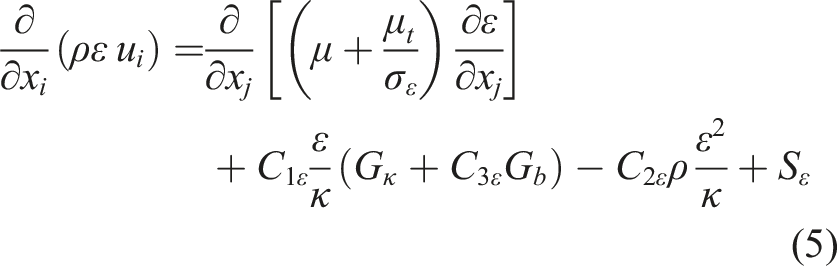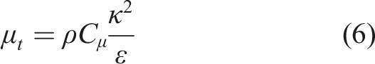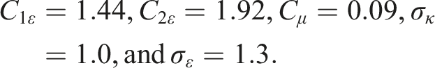Regarding the porous zone, $F = - \frac{μ}{ϕ K} \vec{v}$ represents the resistance to flow in the porous medium (momentum sink), and K is the permeability of the porous medium.

Turbulent flow within the U-shaped pipe

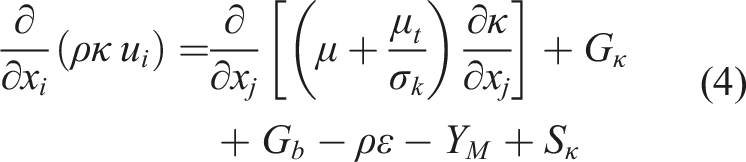
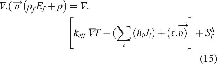
The two-equation turbulence model, such as $κ - ε$ , establishes turbulent length and time scales by independently solving transport equations. The robustness and reasonable accuracy of this model make it prevalent for flow and heat transfer simulations in industrial applications. This model is based on a transport model for turbulence kinetic energy ( $κ$ ) and its dissipation rate (ε). For this study, a modified $κ - ε$ model, known as the RNG $κ - ε$ , is used.⁶⁵

\frac{\partial}{\partial x_{i}} (ρ κ u_{i}) = \frac{\partial}{\partial x_{j}} [(μ + \frac{μ_{t}}{σ_{k}}) \frac{\partial κ}{\partial x_{j}}] + G_{κ} + G_{b} - ρ ε - Y_{M} + S_{κ}

(4)

\frac{\partial}{\partial x_{i}} (ρ ε u_{i}) = \frac{\partial}{\partial x_{j}} [(μ + \frac{μ_{t}}{σ_{ε}}) \frac{\partial ε}{\partial x_{j}}] + C_{1 ε} \frac{ε}{κ} (G_{κ} + C_{3 ε} G_{b}) - C_{2 ε} ρ \frac{ε^{2}}{κ} + S_{ε}

(5)

μ_{t} = ρ C_{μ} \frac{κ^{2}}{ε}

(6)

G_{κ}

is the production of turbulent kinetic energy resulting from variations in average velocity, and

G_{b}

is the generation of turbulent kinetic energy due to buoyancy effect. Also,

Y_{M}

involves the contribution of fluctuating dilation in compressible turbulence to the overall dissipation rate. The constant terms are as follows⁶⁵:

C_{1 ε} = 1.44, C_{2 ε} = 1.92, C_{μ} = 0.09, σ_{κ} = 1.0, and σ_{ε} = 1.3 .

Energy equation for solidification

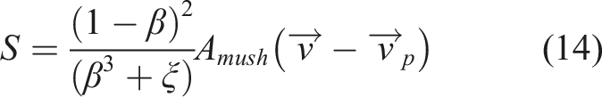
The enthalpy-porosity technique, as referenced in Ref. 66 and implemented in ANSYS FLUENT, approximates the liquid fraction of the cell volume by accounting for the enthalpy balance during each iterative step. Essentially, the Porous Zone model is a momentum equation complemented by an additional source term. The phase transition within the mushy zone incorporates a medium with a fluid fraction range between 0 and 1. During freezing, the liquid phase solidifies and adheres to the solid region, causing the liquid fraction to diminish from 1 to 0. Therefore, the porosity and velocity of the solidified area become 0. The energy conservation equation for solidification/melting is denoted as equation (6).⁶⁷

ρ \nabla . (\vec{v} H) = \nabla . (k_{e f f} \nabla T) + S

(7)

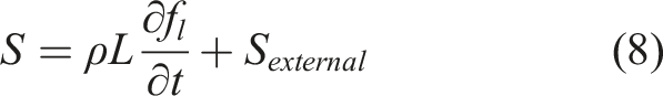
In this study, the source term S in the energy equation represents the latent heat released during the freezing of water in the porous soil and any external heat contributions.

Mathematically, S is expressed as⁶⁸:

S = ρ L \frac{\partial f_{l}}{\partial t} + S_{e x t e r n a l}

(8)

ρ L \frac{\partial f_{l}}{\partial t}

captures the latent heat release per unit volume, where

L

is the latent heat of fusion,

f_{l}

is the liquid fraction and

\frac{\partial f_{l}}{\partial t} = 0

S_{e x t e r n a l}

represents additional heat sources such as geothermal heat flux or heat transfer from the borehole. For steady-state conditions, S reflects the balanced heat exchange due to phase change and any steady heat input, ensuring accurate modeling of freezing and thermal processes in borehole heat exchangers.

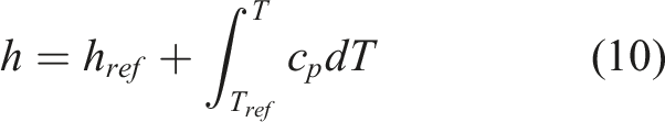
In equation (7), the material total enthalpy (H) is derived by summing the sensible enthalpy $h$ and latent heat $Δ H$ as shown:

H = h + Δ H

(9)

h = h_{r e f} + \int_{T_{r e f}}^{T} c_{p} d T

(10)

ρ

\vec{v}

, and

S

are density, fluid velocity and the source term,⁶⁵ respectively. Also,

h

as the sensible heat enthalpy is equal to the reference enthalpy

h_{r e f}

added to

\int_{T_{r e f}}^{T} c_{p} d T

where

c_{p}

is the specific heat capacity at constant pressure and

T_{r e f}

is the reference temperature.

The second term of equation (7), $Δ H$ ,latent heat content, is computed as equation (9) where $L$ is the latent heat of the material.

Δ H = β L

(11)

where the liquid fraction

β

is defined as following,⁶⁹

\begin{array}{l} β = 0 & T < T_{s o l i d u s} \\ β = 1 & T > T_{l i q u i d u s} \\ β = \frac{T - T_{s o l i d u s}}{T_{l i q u i d u s} - T_{s o l i d u s}} & T_{s o l i d u s s} < T < T_{l i q u i d u s} \end{array}

(12)

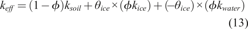
The effective thermal conductivity in the soil can be defined based on equation (11).⁷⁰

k_{e f f} = (1 - ϕ) k_{s o i l} + θ_{i c e} \times (ϕ k_{i c e}) + (- θ_{i c e}) \times (ϕ k_{w a t e r})

(13)

where

θ_{i c e}

is the ice fraction within the soil.

Momentum equation in soil region

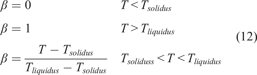
As mentioned, the enthalpy-porosity method considers the partially solidified zone (mushy region) as porous media. The momentum sink due to the reduced porosity in the mushy region is presented as equation (12).⁶⁵

S = \frac{{(1 - β)}^{2}}{(β^{3} + ξ)} A_{m u s h} (\vec{ν} - {\vec{ν}}_{p})

(14)

β

is the liquid fraction,

{\vec{ν}}_{p}

is the solid velocity due to the pulling of solidified material, and

A_{m u s h}

is a constant specific to the mushy region that measures the amplitude of damping, and the term

ξ = 0.001

is included to prevent division by zero.

Energy equation in soil as a porous media

\nabla . (\vec{υ} (ρ_{f} E_{f} + p) = \nabla . [k_{e f f} \nabla T - (\sum_{i} (h_{i} J_{i}) + (\bar{τ} . \vec{υ)}] + S_{f}^{h}

(15)

E_{f}

is the total fluid energy,

E_{s}

is the total solid medium energy,

ϕ

is the porosity of the soil,

k_{e f f}

is the effective thermal conductivity of the medium, and

S_{f}^{h}

is the fluid enthalpy source term.

In this study, $S_{f}^{h}$ represents the energy source term capturing the latent heat exchange during the solidification process in the porous medium.⁶⁶ It accounts for the heat released or absorbed as water freezes within the soil pores, ensuring the energy balance reflects phase change interactions. Additionally, $S_{f}^{h}$ includes contributions from external heat sources, such as geothermal heat flux or heat transfer from the borehole, which are critical for accurately modeling steady-state freezing and heat transfer in the borehole heat exchanger system.

k_{e f f} = ϕ k_{f} + (1 - ϕ) k_{s}

(16)

k_{f}

is the fluid phase thermal conductivity and

k_{s}

is the solid medium thermal conductivity.

The thermal resistance between the borehole wall and working fluid serves as a measure of thermal efficiency of the borehole system. Literature suggests that thermal efficiency is influenced by several factors, such as the fluid flow rate, pipe geometry, pipe material, and the grout type.⁹ Equation (15) presents the total resistance between the soil and pipe, which reflects the temperature difference between the working fluid 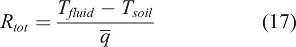$T_{f l u i d}$ and the borehole surrounded wall $T_{s o i l}$ as well as the heat flow between the inlet and outlet of the working fluid $\bar{q}$ .

R_{t o t} = \frac{T_{f l u i d} - T_{s o i l}}{\bar{q}}

(17)

The COP in a GSHP system is defined as the ratio of the energy produced to the energy consumed.⁷¹ The COP of the heat pump regarding heating purposes based on the BHE outlet temperature can be considered as equation (16).^72–74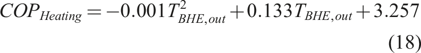

C O P_{H e a t i n g} = - 0.001 T_{B H E, o u t}^{2} + 0.133 T_{B H E, o u t} + 3.257

(18)

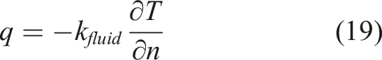
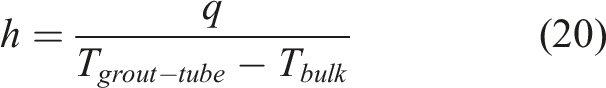
Nusselt number (Nu) was calculated to evaluate the heat transfer performance between the U-tube and the grout, with $N u_{a v e} = \frac{1}{A} \int_{A} N u d A$ obtained by integrating local Nu values along the tube-grout boundary.⁶⁵ The calculation procedure is provided as follows.

q = - k_{f l u i d} \frac{\partial T}{\partial n}

(19)

where (q) is the heat flux at the wall based on the temperature gradient.

h = \frac{q}{T_{g r o u t - t u b e} - T_{b u l k}}

(20)

To find the heat transfer coefficient (h), use the heat flux and temperature difference between the wall and bulk fluid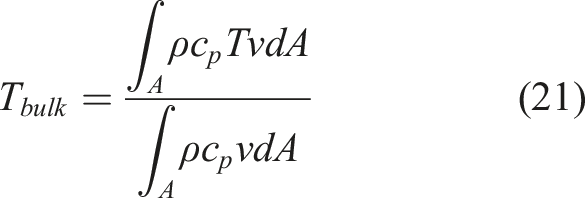

T_{b u l k} = \frac{\int_{A} ρ c_{p} T v d A}{\int_{A} ρ c_{p} v d A}

(21)

Calculates the fluid’s average temperature across the cross-section.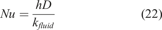

N u = \frac{h D}{k_{f l u i d}}

(22)

Combines the heat transfer coefficient (h), hydraulic diameter (D), and fluid thermal conductivity.

Depth-dependent ground temperature variations

As mentioned, soil temperature varies across the ground depth at each location. This variation is incorporated into the model through a user-defined function code for the sidewalls of the soil as a boundary condition. Equation (17) represents the ground temperature profile based on time and depth.⁴⁶

T (z, t) = \bar{T_{s}} + A_{s} . \exp (- z \sqrt{\frac{π}{α t_{0}}}) \cos (\frac{2 π t}{t_{0}} - z \sqrt{\frac{π}{α t_{0}}})

(23)

\bar{T_{s}}

is the annual average ground surface temperature that can be calculated based on equation (18).⁷⁵

\bar{T_{s}} = 17.898 + 0.951 {\bar{T}}_{a m b}

(24)

A_{s}

represents half of the difference between the minimum and maximum temperatures for the period,⁷⁶

α

is the thermal diffusivity of the soil (m²/day), and

t_{0}

is the number of days in a complete cycle (365 days).

Table 6 indicates the thermal diffusivity, annual average ground surface temperature, and temperature amplitude during a complete cycle for each location used in this study.

Table 6.

Parameters used in equation (23).

Location	$α$ (m²/day)	${\bar{T}}_{a m b}$ (K)	A_s (K)
AB⁴⁹	0.0566	279.50	35.34
BC⁵⁰	0.0561	283.41	24.63
PE⁵¹	0.0803	279.83	26.93
MN⁵²	0.0573	277.16	35.85
NB⁵³	0.0607	279.00	27.50
NS⁵⁴	0.0580	279.83	25.39
ON⁵⁵	0.0637	280.58	34.50
QC⁵⁶	0.0628	280.33	28.99
SK⁵⁷	0.0789	273.77	38.00

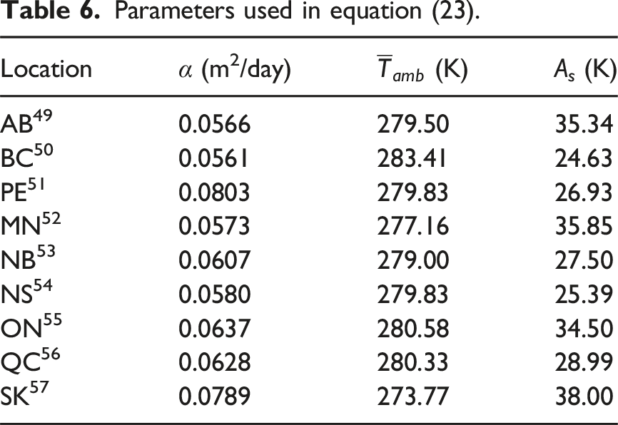
Figure 4 illustrates the temperature fluctuations over time (from Dec 2021 to Feb 2022) and ground depth at the AB location. The phenomenon where the maximum temperature occurs at certain depths (1–10 m) during winter months is influenced by the heat penetration from the previous summer. This occurs due to the thermal inertia of the soil, causing a lag in the temperature response to surface temperature changes. The heat from the summer penetrates the ground and continues to propagate downward, resulting in a temperature maximum at certain depths during the winter, known as thermal or seasonal lag which is also confirmed in experimental measurements as well.^75,77,78 At this site, a representative average temperature profile for the winter season was determined at the end of January 2022 (as shown by the dashed-line profile). Given the different parameters involved in equation (17), customized average temperature profiles are calculated for each geographical location. These temperature profiles are ultimately loaded as UDF codes for the soil sidewall boundary conditions through the ground depth.

Figure 4.

(a) Temperature profile in winter season versus time and ground depth at the AB location, (b) corrected final temp profile at the AB location.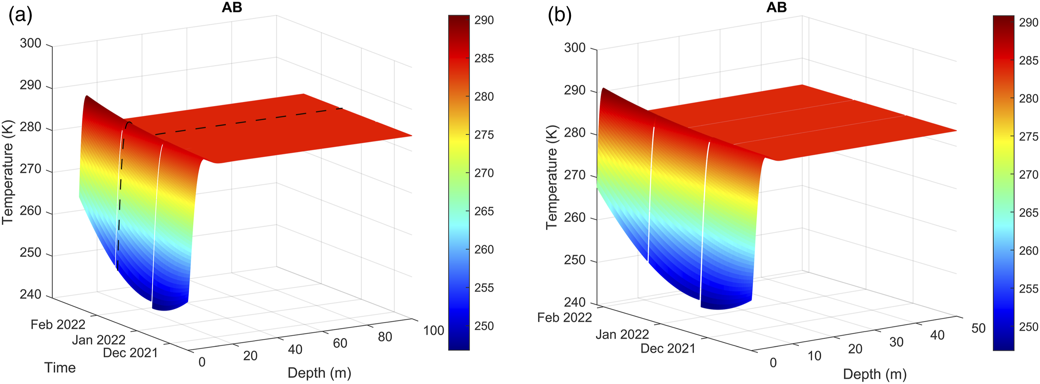

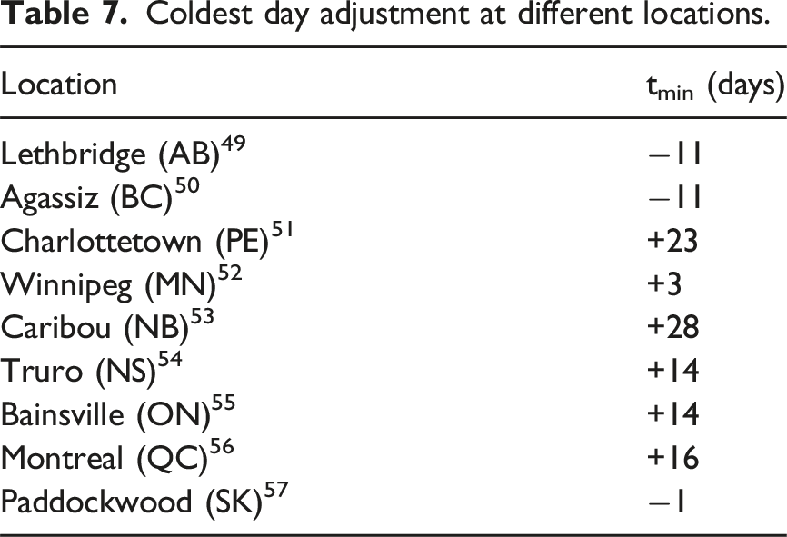
Temperature profile development on the coldest day

Based on equation (17), the coldest day of a complete 365-day cycle should be the first day of the cycle due to the presence of

\cos (\frac{2 π t}{t_{0}} - z \sqrt{\frac{π}{α t_{0}}})

term. In this study, the first day of the cycle is January 1^st. However, in reality, the minimum temperature may not occur on the first day of the cycle. Therefore, equation (17) is revised to account for how much the coldest day deviates from January 1^st during the winter season. In this context, January 1^st, 2022 is set as a reference day, with December 2021 represented by a negative sign and January and February 2022 by a positive sign. For example, according to Table 7, the coldest day in winter in Alberta was the 19^th of December 2021, which is 11 days before January 1^st, 2022 (indicating

t_{\min} = - 11

). Conversely, in Ontario, the coldest winter was the 14th of January 2022 (indicating

t_{\min} = + 14

). This modified equation (19) will shift the plot presented in Figure 5(a) so that the minimum surface temperature corresponds with the coldest day (shown in Figure 5(b)). The temperature profiles for other locations are presented in Supplemental information.

T_{\min} (z, t) = {\bar{T}}_{s} + A_{s} . \exp (- z \sqrt{\frac{π}{α t_{0}}}) \cos (\frac{2 π (t + t_{\min})}{t_{0}} - z \sqrt{\frac{π}{α t_{0}}})

(25)

Table 7.

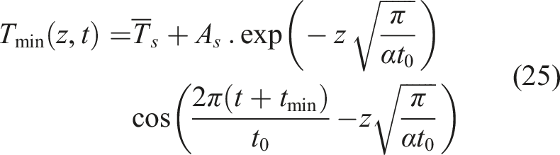
Coldest day adjustment at different locations.

Location	t_min (days)
Lethbridge (AB)⁴⁹	−11
Agassiz (BC)⁵⁰	−11
Charlottetown (PE)⁵¹	+23
Winnipeg (MN)⁵²	+3
Caribou (NB)⁵³	+28
Truro (NS)⁵⁴	+14
Bainsville (ON)⁵⁵	+14
Montreal (QC)⁵⁶	+16
Paddockwood (SK)⁵⁷	−1

Figure 5.

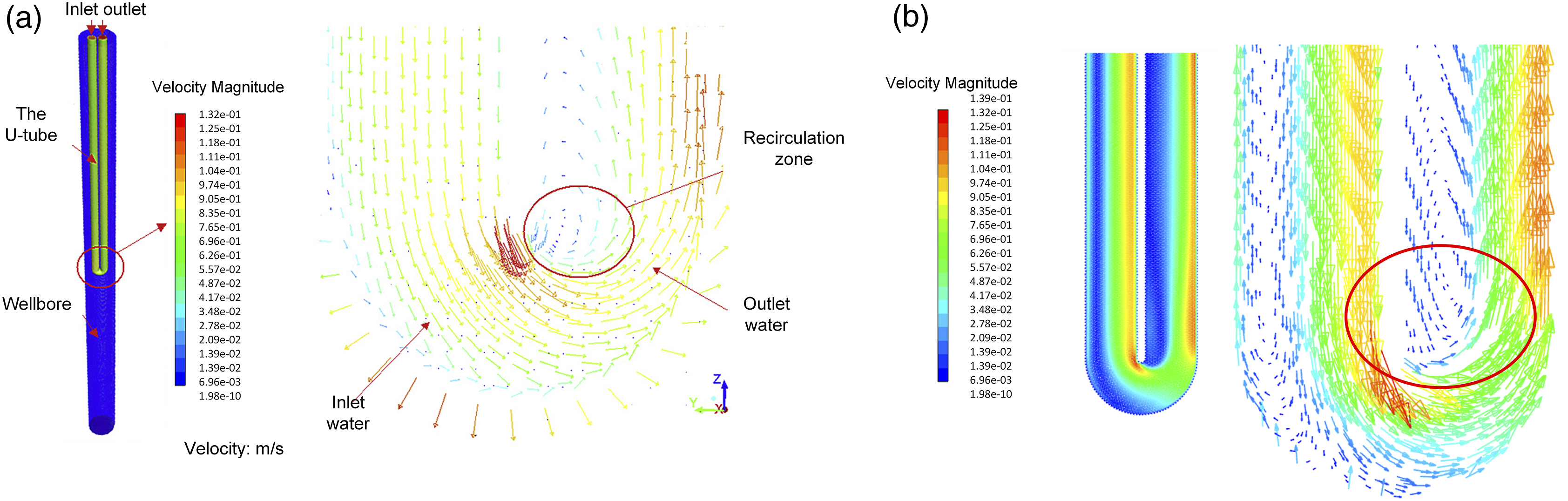
Velocity vectors comparison (m/s) using $κ - ε$ turbulent model: (a) previous work⁷⁹ and (b) current study.

Validation

Turbulent flow and solidification within porous media are two basic phenomena governing the simulation processes. To our knowledge, similar studies that consider both governing equations in borehole simulations are lacking. Consequently, the validation process was bifurcated into two steps: hydrodynamics validation and solidification model verification. The simulation of turbulent water flow within a U-tube situated underground was implemented using the k-ɛ realizable turbulent model⁷⁹ to confirm the validity of the turbulent model in the current study. 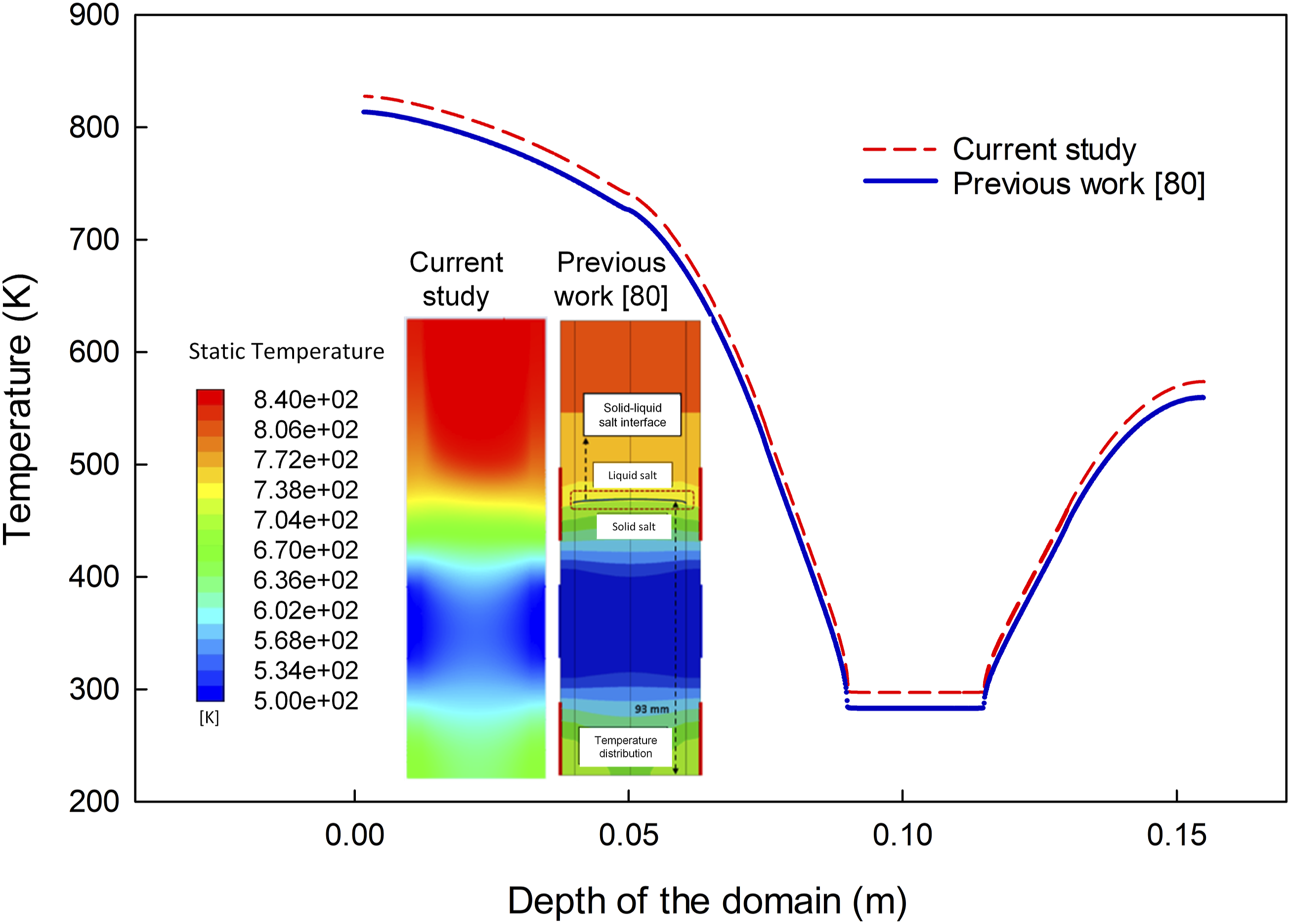As shown in Figure 5, the resultant velocity data illustrated a great agreement with existing literature.⁷⁹ In addition, to verify the reliability of the solidification model, the current study was validated against a work,⁸⁰ which simulated the freezing performance in a molten salt reactor. As shown in Figure 6, the solid-liquid interface in the current study is clearly defined and consistent with the previous study. The liquid fraction gradient transitions smoothly from liquid to solid, aligning well with previous results. This agreement validates the robustness of the phase change model in predicting the freezing process. In addition, the temperature profile along the depth of the domain (wall) and temperature contours for the whole domain is presented in Figure 7 for both the current study and the previous study.⁸⁰ Both profiles show a similar trend with strong consistency throughout the depth, confirming that the thermal gradients and freezing process have been accurately captured in the current model, with an error margin below 5%.

Figure 6.

Comparison of liquid fraction contours: Previous⁸⁰ versus current study.

Figure 7.

Comparison of the temperature profile (K) and temperature contour (K): Previous⁸⁰ versus current study.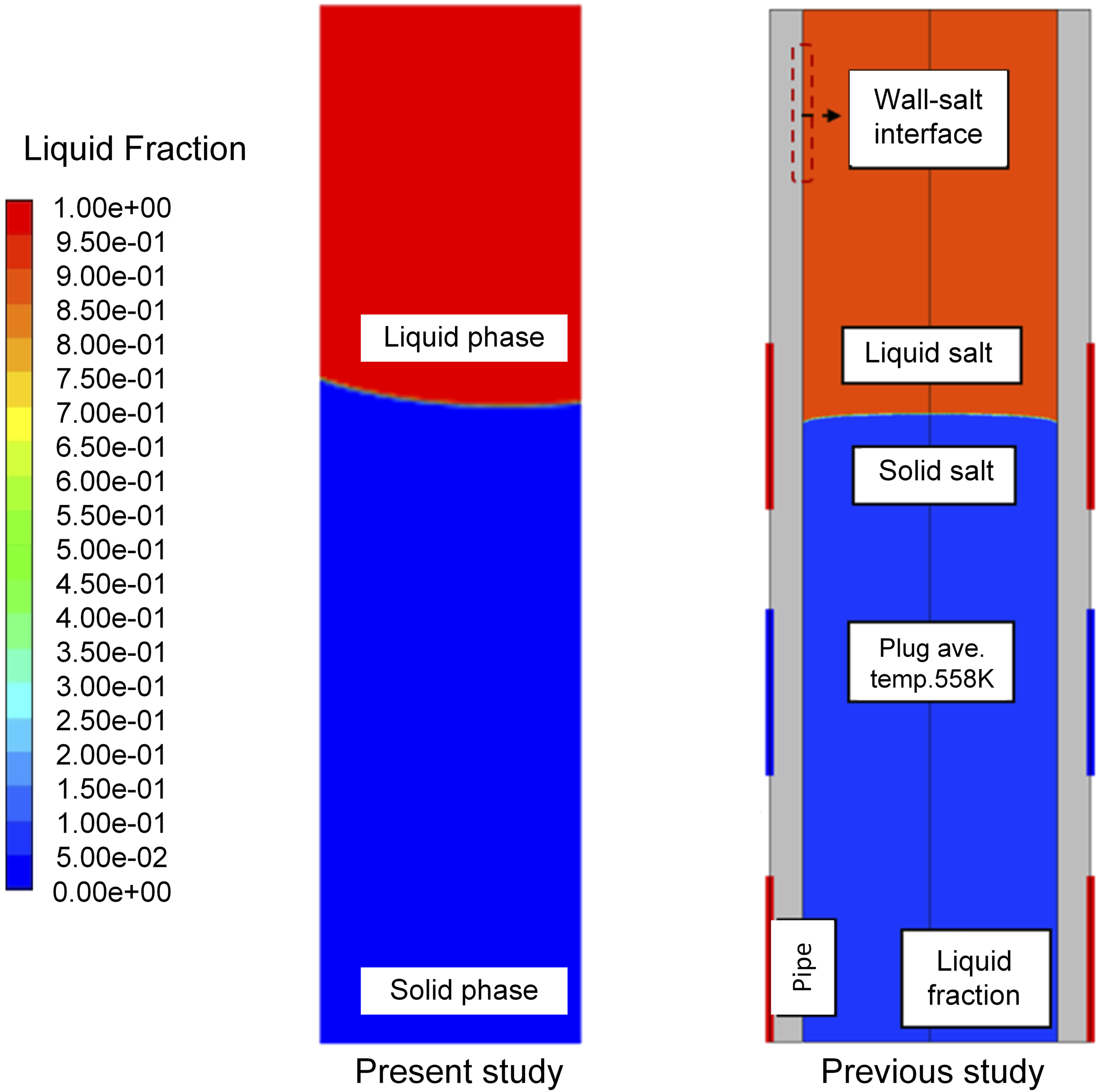

Mesh independence analysis

The geometry and mesh were created using GAMBIT 2.4.6 software, with the resulting mesh structure displayed in Figure 8. The mesh element numbers were improved step-by-step as presented also in Figure 8. The ice formation fraction and total thermal resistance were considered as comparative outcomes. The mesh dependence test process indicates that to achieve a difference of less than 0.05% in ice formation, thermal resistance, temperature, and Nu number the optimal number of mesh elements is 728,000, which was the chosen number for the simulations.

Figure 8.

(a) Mesh structure at the last 2 m of the BHE system, Mesh independence analysis in MN (b1) Ice formation fraction and thermal resistance (b2) Temperature variations of tube-grout boundary at different depths (b3) Nusselt number variations of tube-grout boundary at different depths.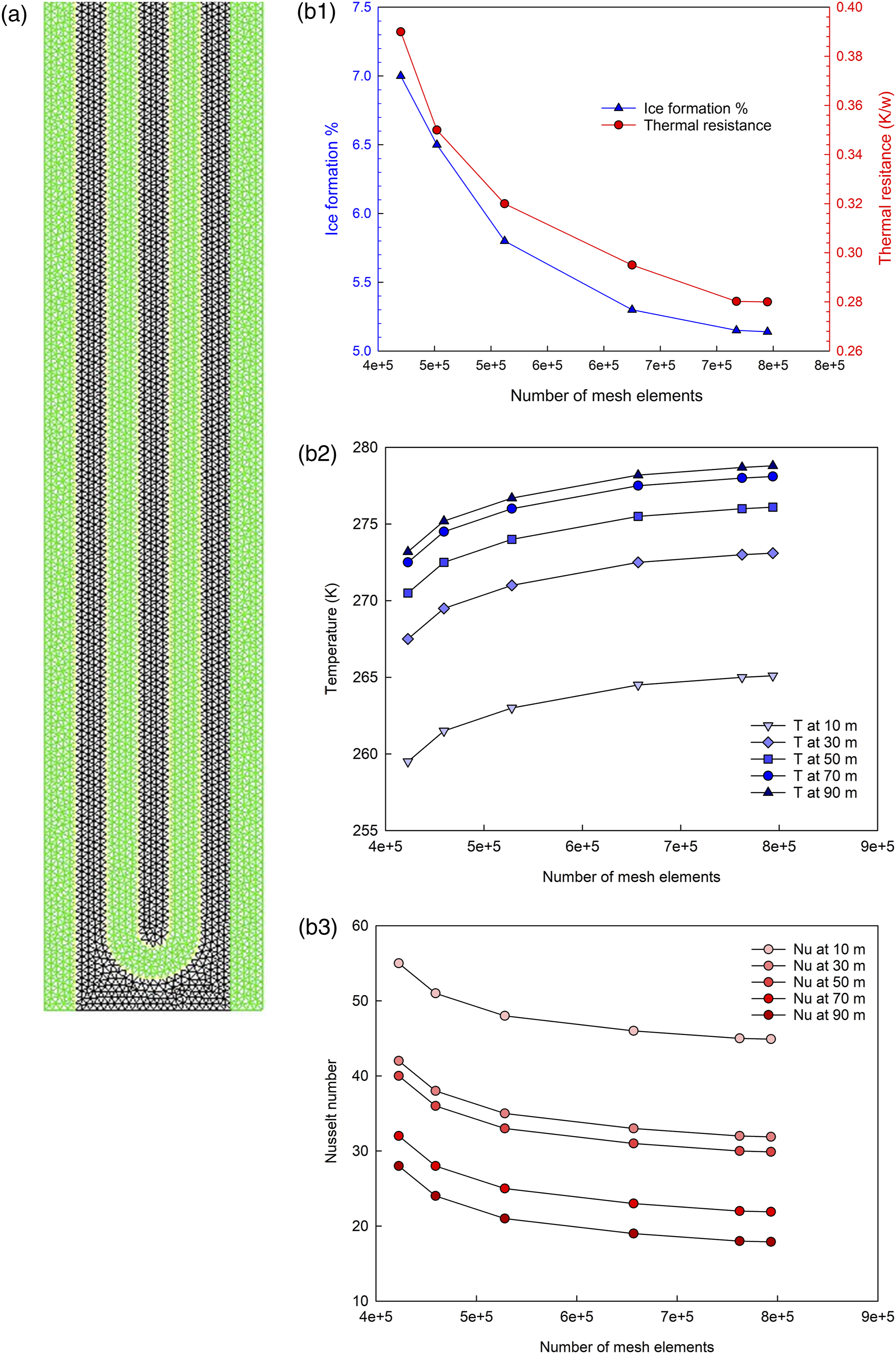

In this study, the mesh was refined to achieve a Y+ value of approximately 25 near the solid-fluid and solid-solid interfaces, such as the grout-tube and grout-soil boundaries. This choice ensures that the wall-adjacent cells lie within the buffer region of the boundary layer, making it more suited for enhanced wall treatment and balancing computational efficiency and improved near-wall resolution. Although the RNG k−ϵ turbulence model typically allows for Y+ values in the range of 30–300 with wall functions,⁸¹ the lower Y+ value enhances the accuracy of thermal and flow predictions near critical interfaces,⁸² such as those involved in ice formation and heat transfer.

Results and discussion

The outcomes of this study, which include simulations of ninety cases, are centered on the impacts of varying soil porosities, thermal conductivities, as well as extreme weather conditions on soil ice formation and borehole efficiency. In addition, the results of the cases dedicated to the nine different locations in Canada during winter are presented. The velocity, temperature, and liquid fraction contours are also illustrated in this section.

Ice formation

The findings regarding the percentage of ice fraction and the outlet temperature of the working fluid of the BHE in different locations, under both average weather in winter and coldest weather scenarios, are presented in Figure 9. Generally, less ice formation results in higher outlet fluid temperature. This is because ice, having a higher thermal conductivity (2.1 W/mK) than water (0.6 W/mK), provides higher effective thermal conductivity and thus enhances heat transfer between the freezing soil and the U-tube near the outlet. Under the coldest conditions in all locations, the level of ice formation in the soil exceeds that in the average weather in winter cases due to the lower temperatures applied in the boundary conditions, thereby reducing the outlet temperature.

Figure 9.

Comparative analysis of ice fraction percentage and BHE fluid outlet temperature (K) across different locations under both average and coldest winter scenarios.

In BC, where the least amount of ice forms, the outlet fluid temperature within the U-tube is maximized. The rate of ice formation increases gradually in BC, QC, PE, ON, and NS locations, varying from 0% to 1.1%. However, it significantly rises in AB, NB, MN, and SK, ranging from 1.50% to 2.60% under average winter conditions. Specifically, the maximum ice formation (3.72%) occurs in SK under the coldest conditions, leading to a minimum temperature difference (9.23 K) between the inlet and outlet of the U-tube.

Figure 10 illustrates the liquid fraction contour within the first 3.3 m of the soil at the SK location, demonstrating the profile of ice formation. This larger view of the ice formation profile, along with the corresponding temperature contour in this section, confirms that the temperature at the ice-saturated soil interface follows the temperature profile. Although the temperature profile applied to the soil on both sides of the BHE is identical (as per the UDF boundary condition), the low temperature of the inlet flow (263 K) induces continuous ice formation along the grout-soil interface (∼10 m) on the left side of the BHE. However, the elevated temperature of the working fluid within the U-tube limits ice formation at the grout-soil interface on the right side to 2.3 m.

Figure 10.

(a) Ice formation contour within the first 3.3 m; (b and c) zoomed-in views of the ice formation profile; (d) temperature profiles corresponding to (a) (SK, winter).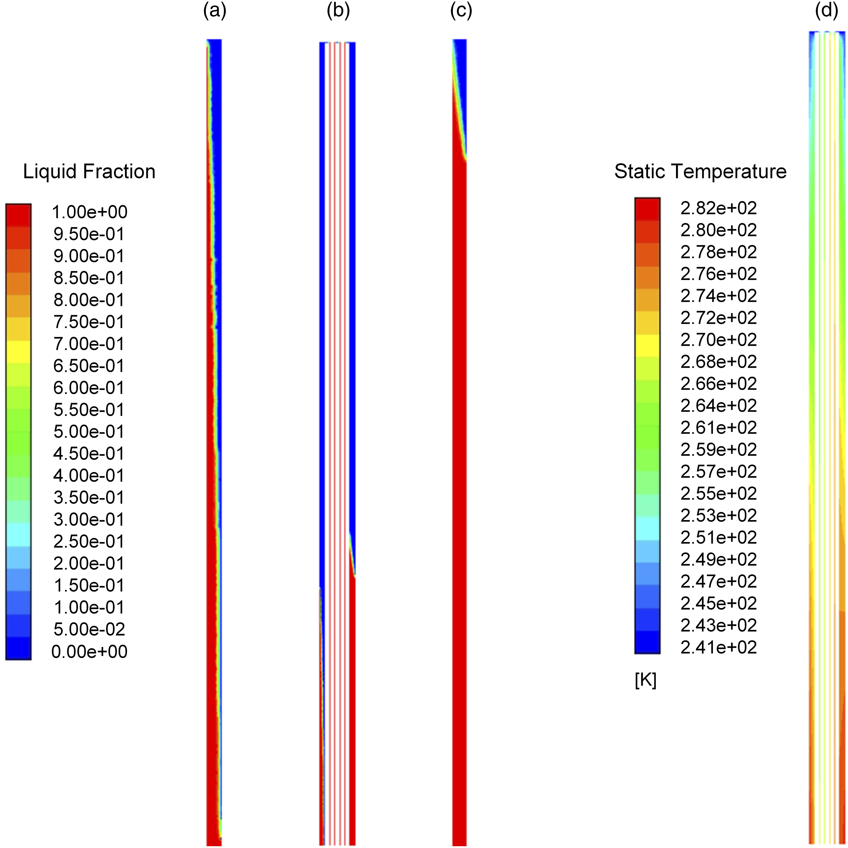

Temperature distribution

Figure 11 presents the temperature distribution contour for the first 6 m, 57-63 m, and the last 6 m of the BHE in the soil, grout, pipe, and the entire system at the AB location. The surface of the soil and grout is exposed to a cold temperature (T = 252.68 K), which is lower than the fluid inlet temperature (T = 263 K) of the U-tube. The average temperature of the BHE system increases with depth due to the corresponding rise in soil temperature shown in Figure 4. Essentially, the average temperature of all zones on the right side of the BHE is higher than that on the left side. As a bilateral medium in heat transfer, the grout is responsible for transferring heat from the soil to the U-tube. The temperature of the fluid in the U-tube improves along the tube due to the heat transfer between tube-grout-soil. The lower temperature of the working fluid results in a lower grout temperature profile, indicating a higher heat transfer rate on the left side. Hence, the temperature of the grout is higher on the right side of the BHE due to the higher temperature of the working fluid in this area. The fluid temperature stabilizes beyond a depth of 6 m due to the consistent thermal environment in deeper soil layers. From the heat transfer perspective, ground temperatures typically stabilize at depths beyond 5–10 m and are less influenced by surface temperature fluctuations. This is a well-documented phenomenon in geothermal and ground energy studies.⁸³ As a result, the thermal gradient driving heat transfer between the fluid and the soil becomes nearly constant. The applied UDF for the boundary condition reflects this stabilization of soil temperature beyond 6 m, making it reasonable for the fluid temperature to remain steady. In the first few meters of the BHE, the temperature difference between the fluid and the surrounding soil is large, causing significant heat transfer. Beyond 6 m, the temperature difference narrows due to soil temperature stabilization and the fluid heating up in the upper sections of the borehole. This results in a lower rate of heat transfer and leads to stabilization in fluid temperature at higher depths. Even if the temperature appears stable in simulations, heat exchange is still occurring, although at a smaller rate.

Figure 11.

Temperature contour of the BHE system across all zones - soil, grout, and U-tube - in (a) the first 6 m, (b) the section from 57 to 63 m, and (c) the final 6 m (94–100 m) during the winter season in AB.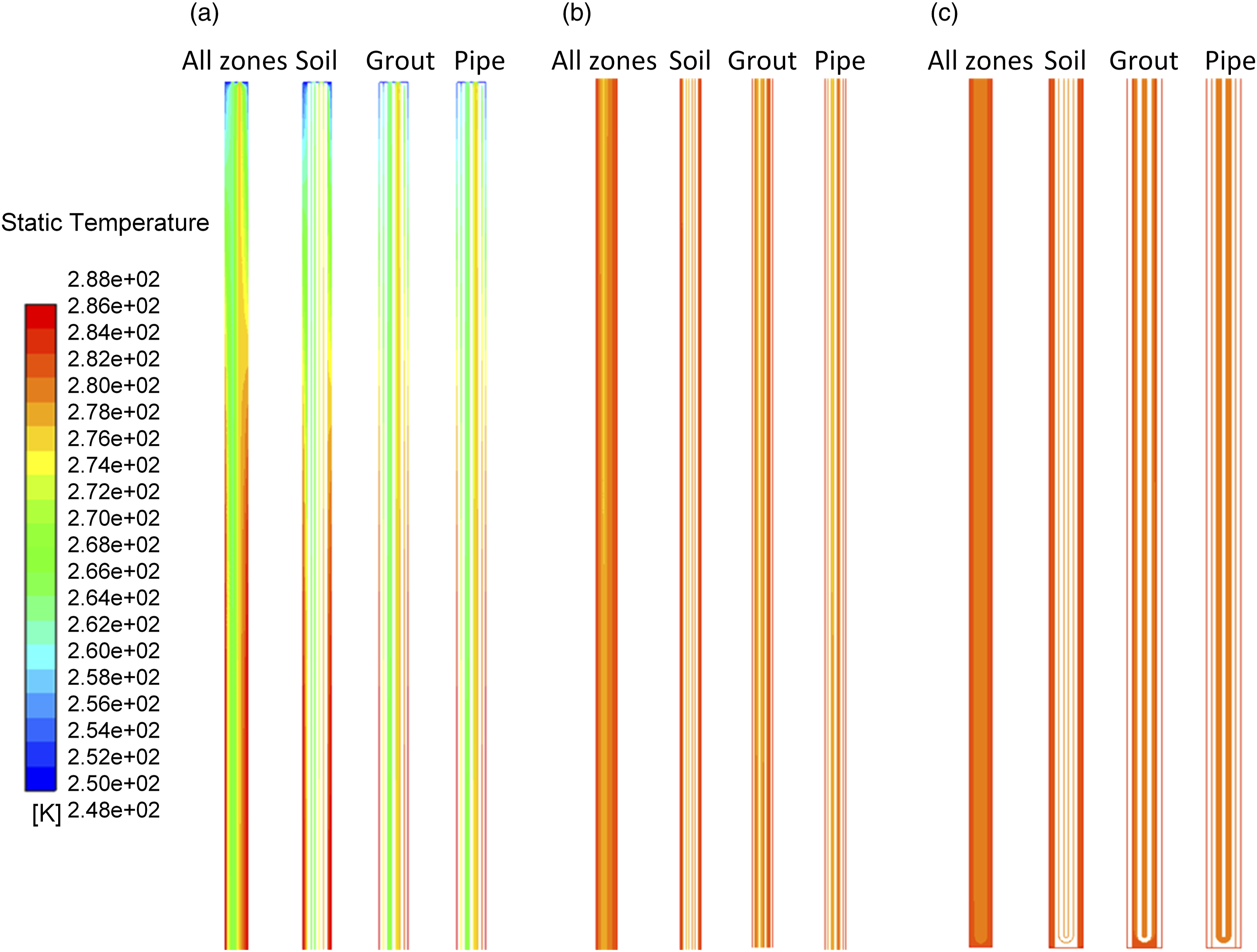

From the design perspective, boreholes serve as a medium for seasonal thermal storage. During summer, heat rejected into the ground can be stored at deeper levels, enhancing heat pump efficiency in winter. A shallow borehole would limit this storage capacity. This depth ensures the system meets design standards for residential applications,^37,38 and supports future scalability for higher loads or longer operational lifetimes. A deeper borehole ensures the system reaches layers where soil remains unfrozen and thermally active.

Impact of soil porosity

Soil porosity plays a critical role in heat transport within the BHE system. As illustrated by equation (13), soil porosity directly influences factors related to k_soil, k_ice, and k_water. Essentially, a higher porosity in saturated soil indicates more available spaces for water and ice within the soil medium, hence influencing the heat exchange process. Figure 12 shows the effects of varying the soil porosity, ranging from 0.4 to 0.55 - a typical range for Canadian soils – on ice formation and the fluid outlet temperature. Thermal conductivity was kept constant, corresponding to the thermal properties specific to each location. The trends for ice formation and outlet temperature in all porosities align with those seen in the average winter scenarios. The data suggests that increased soil porosity allows for more void spaces for water, resulting in an enhanced likelihood of ice formation within the BHE system. These effects are particularly noticeable in the AB, NB, MN, and SK locations. Therefore, it is deduced that during winter, lower soil porosities yield higher fluid outlet temperatures, underscoring the significant role of soil porosity on the system’s thermal performance.

Figure 12.

Variations in ice formation percentage and fluid outlet temperature (K) across all locations, based on changes in (a) soil porosity, (b) soil thermal conductivity.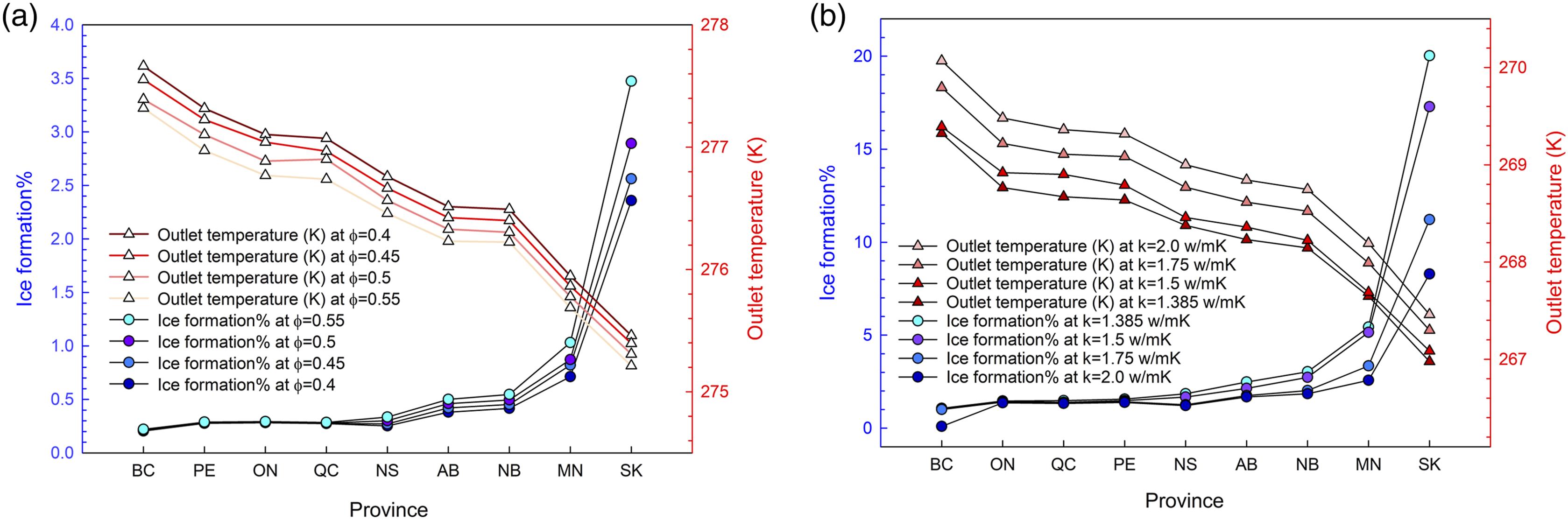

Impact of thermal conductivity

The thermal conductivity of the soil plays an active role in the heat transfer process among different zones in the BHE system. As suggested by equation (13), the effective thermal conductivity is influenced by variations in soil thermal conductivity. The results of ice formation in the soil and outlet fluid temperature based on soil thermal conductivity variations for each location from 1.385 w/mK to 2.0 w/mK are also plotted in Figure 12. For these simulations, soil porosity is held constant equal to the real porosity in each location. The ice formation and outlet temperature trends for each location align with those of the actual cases (shown in Figure 9), featuring their respective real soil thermal conductivity.

Generally, a lower soil thermal conductivity leads to an increase in ice formation within the soil medium and a decrease in the fluid outlet temperature. The impact of thermal conductivity variations on ice formation is particularly significant in locations such as MN and SK. Therefore, it can be inferred that the higher soil thermal conductivity is in favor of achieving less ice formation and higher outlet temperature in the BHE system.

COP of the heat pump

The variation in the COP of the heat pump relative to the outlet fluid temperature from the BHE system is illustrated in Figure 13. From equation (16), it is evident that the COP is directly proportional to the outlet fluid temperature of the BHE. Consequently, in locations like BC, where the BHE system produces the highest temperature fluid to enter the heat pump, the corresponding COP is maximized. Conversely, in SK, recognized as the coldest region, the output fluid temperature is lowest, leading to the smallest COP for the corresponding heat pump. In addition, since the outlet temperature of the working fluid on the coldest days is less than average winter cases, the COP of the heat pump tends to be lower on coldest days compared to the average COP values during winter across all Canadian locations. These findings have profound implications for the widespread adoption of geothermal heating systems, particularly in high-density energy-use districts where efficient heat pumps can substantially reduce energy use and greenhouse gas emissions.

Figure 13.

COP of the heat pump added to the BHE and the outlet fluid temperature (K) at different locations.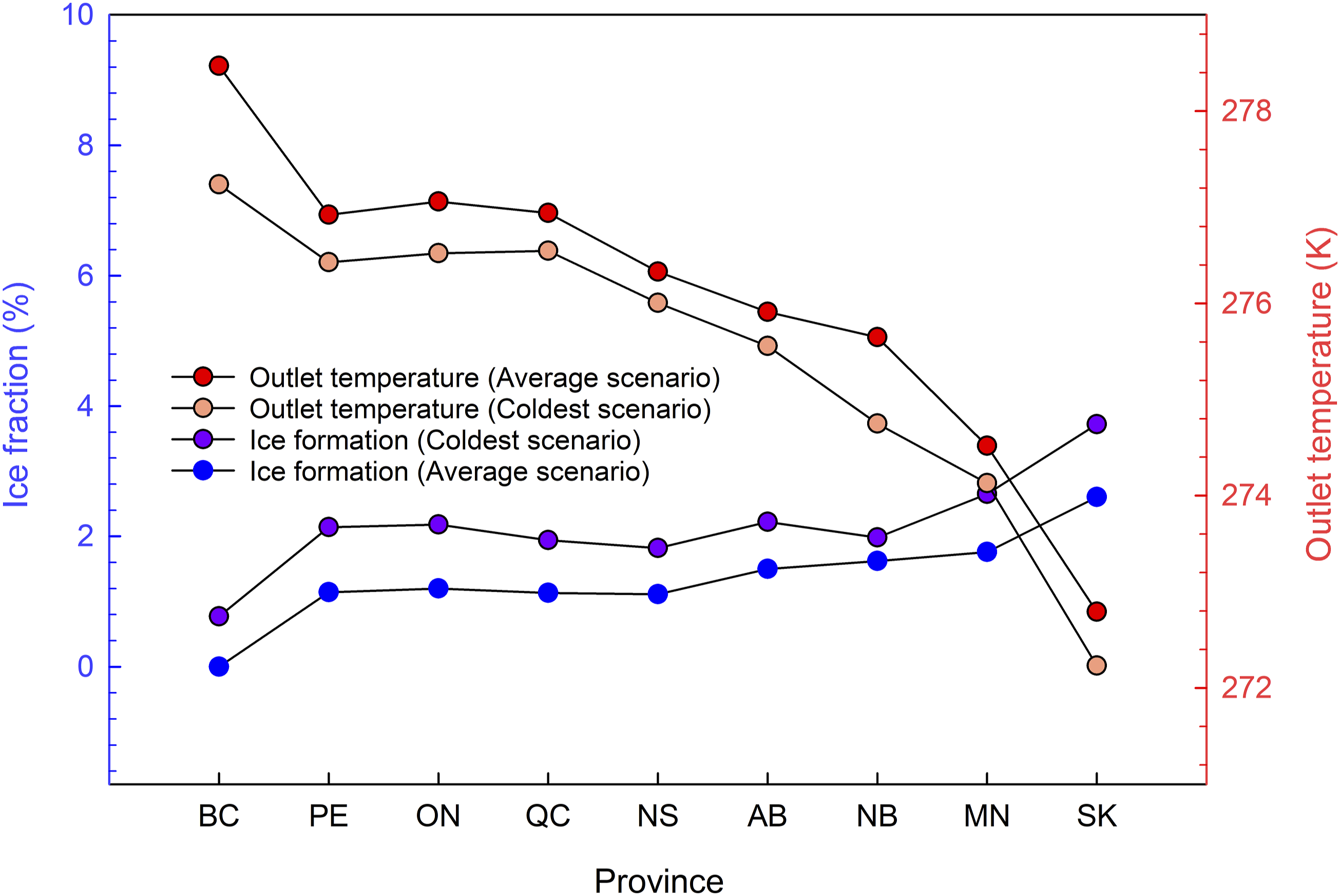

Conclusion

This study employed CFD methods to explore ice formation within the soil and thermal resistance in nine different geographical locations across Canada during winter. Also, this research evaluated the influence of soil thermal conductivity, soil porosity, and extreme cold conditions in a total of 90 scenarios.

The findings shed light on several crucial insights:

- The maximum occurrence of ice formation was recorded in Paddockwood (SK), exceeding 8 %, due to the cold average surface temperature in winter (T = 244.94 K). Conversely, Agassiz (BC) exhibited the minimum ice formation (2%), owing to the relatively warm average winter temperature of 265.03 K.

- Lethbridge (AB) and Central Manitoba (MN) presented the highest thermal resistance among all locations examined. In contrast, Paddockwood (SK) and Charlottetown (PE) demonstrated the lowest resistance, making them the most thermally efficient sites for borehole systems.

- By increasing the soil porosity, the average ice formation within the soil faced a gradual increase in all cases as a result of more available spaces for water and ice within the soil medium.

- Higher soil thermal conductivity is in favor of achieving less ice formation and higher outlet temperature in the BHE system.

- Paddockwood (SK) emerged as the location most sensitive to variations in thermal conductivity, possessing the least porosity and highest thermal conductivity among all sites considered.

- Extreme cold weather, characterized by lower temperatures, triggered increased ice formation in all locations, with the maximum ice formation fraction observed in Paddockwood (SK).

- The BHE system in the BC location generated fluid with the highest temperature for the heat pump, resulting in the highest corresponding COP in this location.

- Using one-way ANOVA, we determined that porosity has a significantly stronger impact on both ice formation and outlet temperature compared to thermal conductivity (k (W/mK)). This conclusion is based on porosity’s much smaller p-values and higher F-statistics in the ANOVA results, indicating a greater effect on the dependent variables.

This study sheds light on the influence of diverse soil and climatic factors on the effectiveness of BHE systems under various weather conditions, providing essential guidance for planning and optimizing such systems across Canada. The outcomes highlight the potential for extensive geothermal energy deployment in regions with high-density energy use, even within frigid climate zones, aiding global efforts toward fulfilling energy requirements via sustainable avenues. Future works can be addressed the full domain size by expanding the model of the thermal plume and heat transfer processes. More research focused on the ideal configuration and operation of geothermal heat exchangers and heat pumps, considering the variations in soil and climatic conditions, may further enrich the knowledge base that informs the design and execution of geothermal heating and cooling networks.

Supplemental Material

Supplemental Material - Impact of soil freezing on the thermal performance of geothermal borehole heat exchangers across Canadian climates

Supplemental Material for Impact of soil freezing on the thermal performance of geothermal borehole heat exchangers across Canadian climates by Fatemeh Keramat and Lexuan Zhong in Building Services Engineering Research & Technology.

Footnotes

Declaration of conflicting interests

The author(s) declared no potential conflicts of interest with respect to the research, authorship, and/or publication of this article.

Funding

The author(s) disclosed receipt of the following financial support for the research, authorship, and/or publication of this article: This study was funded by the Canada First Research Excellence Fund as part of the University of Alberta’s Future Energy Systems initiative (CFREF-2015-00001).

ORCID iD

Lexuan Zhong

Supplemental Material

Supplemental material for this article is available online.

Appendix

References

Alavy

Shirazi

Rosen

. Long-term energy performance of thermal caisson geothermal systems. Energy Build 2023; 292: 113152.

Hakkaki-Fard

Aidoun

Ouzzane

. Applying refrigerant mixtures with thermal glide in cold climate air-source heat pumps. Appl Therm Eng 2014; 62(2): 714–722.

Javadi

Mousavi Ajarostaghi

Rosen

, et al. Performance of ground heat exchangers: a comprehensive review of recent advances. Energy 2019; 178: 207–233.

Gamage

. Numerical methodology for feasibility analysis of ground source heat pumps. Ankara, Türkiye: Middle East Technical University, 2014.

Maghrabie

Abdeltwab

Tawfik

MHM

. Ground-source heat pumps (GSHPs): materials, models, applications, and sustainability. Energy Build 2023; 299: 113560.

Ahmed

Assadi

Kalantar

, et al. A critical review on the use of shallow geothermal energy systems for heating and cooling purposes. Energies 2022; 15(12): 4281.

Sliwa

Sapińska-Śliwa

Gonet

, et al. Geothermal boreholes in Poland—overview of the current state of knowledge. Energies 2021; 14(11): 3251.

Mogensen

. Fluid to duct wall heat transfer in duct system heat storages. Doc Swed Counc Build Res. 1983; (16): 652–657.

Badenes

Mateo Pla

MÁ

Magraner

, et al. Theoretical and experimental cost–benefit assessment of borehole heat exchangers (BHEs) according to working fluid flow rate. Energies 2020; 13(18): 4925.

10.

Vella

Borg

Micallef

. The effect of shank-space on the thermal performance of shallow vertical U-tube ground heat exchangers. Energies 2020; 13(3): 602.

11.

Dalla Santa

Galgaro

Sassi

, et al. An updated ground thermal properties database for GSHP applications. Geothermics 2020; 85: 101758.

12.

Fujii

Okubo

Nishi

, et al. An improved thermal response test for U-tube ground heat exchanger based on optical fiber thermometers. Geothermics 2009; 38(4): 399–406.

13.

Xia

Gong

, et al. Recent advances and development in optimal design and control of ground source heat pump systems. Renew Sustain Energy Rev 2020; 131: 110001.

14.

, et al. Optimization on the performance of ground heat exchangers for GSHP using Kriging model based on MOGA. Appl Therm Eng 2017; 118: 480–489.

15.

Zhou

Mao

, et al. Performance assessment and techno-economic optimization of ground source heat pump for residential heating and cooling: a case study of Nanjing, China. Sustain Energy Technol Assessments 2020; 40: 100782.

16.

Serageldin

Sakata

Katsura

, et al. Thermo-hydraulic performance of the U-tube borehole heat exchanger with a novel oval cross-section: numerical approach. Energy Convers Manag 2018; 177: 406–415.

17.

Koenig

. Thermal resistance of borehole heat exchangers composed of multiple loops and custom shapes. Geothermal Energy 2015; 3: 10–14.

18.

Kerme

Fung

. Comprehensive simulation based thermal performance comparison between single and double U-tube borehole heat exchanger and sensitivity analysis. Energy Build 2021; 241: 110876.

19.

Tang

Nowamooz

. Factors influencing the performance of shallow borehole heat exchanger. Energy Convers Manag 2019; 181: 571–583.

20.

Hein

Kolditz

Görke

, et al. A numerical study on the sustainability and efficiency of borehole heat exchanger coupled ground source heat pump systems. Appl Therm Eng 2016; 100: 421–433.

21.

Qian

Wang

. Modeling the interactions between the performance of ground source heat pumps and soil temperature variations. Energy Sustain Dev 2014; 23: 115–121.

22.

Zhang

Rhee

K-N

Jung

G-J

. Mock-up experimental study on the performance of a combined cooling-domestic hot water-ground source heat pump system. Build Serv Eng Res Tecnol 2023; 44(2): 187–209.

23.

Nikitin

Deymi-Dashtebayaz

Muraveinikov

, et al. Comparative study of air source and ground source heat pumps in 10 coldest Russian cities based on energy-exergy-economic-environmental analysis. J Clean Prod 2021; 321: 128979.

24.

Hakkaki-Fard

Eslami-Nejad

Aidoun

, et al. A techno-economic comparison of a direct expansion ground-source and an air-source heat pump system in Canadian cold climates. Energy 2015; 87: 49–59.

25.

Eslami-nejad

Bernier

. Freezing of geothermal borehole surroundings: a numerical and experimental assessment with applications. Appl Energy 2012; 98: 333–345.

26.

Zheng

Shao

Schelenz

, et al. Efficiency and economic analysis of utilizing latent heat from groundwater freezing in the context of borehole heat exchanger coupled ground source heat pump systems. Appl Therm Eng 2016; 105: 314–326.

27.

Anbergen

Rühaak

Frank

, et al. Numerical simulation of a freeze–thaw testing procedure for borehole heat exchanger grouts. Can Geotech J 2015; 52(8): 1087–1100.

28.

Cao

Bottarelli

Bortoloni

, et al. Small-scale lab analysis of the ground freezing effect on the thermal performance of a Flat-Panel ground heat exchanger. Geothermics 2018; 74: 247–254.

29.

Zhang

Han

, et al. Study on the influence of borehole spacing considering groundwater flow and freezing factors on the annual performance of the ground source heat pump. Appl Therm Eng 2021; 182: 116042.

30.

Yan

Gao

, et al. Characteristics of ground source heat pump considering soil freezing process in cold regions. Energy Build 2023; 297: 113460.

31.

Yang

Zhou

, et al. Experimenting and modeling thermal performance of ground heat exchanger under freezing soil conditions. Sustainability 2019; 11(20): 5738.

32.

Dalla Santa

Farina

Anbergen

, et al. Relevance of computing freeze-thaw effects for borehole heat exchanger modelling: a comparative case study. Geothermics 2019; 79: 164–175.

33.

Kazemi

Roostaie

Egorov

, et al. An analytical solution for heat extraction from shallow ground using a single-phase closed thermosyphon: a model for artificial ground freezing. J Energy Storage 2022; 55: 105599.

34.

Yang

Kong

Chen

. Numerical evaluation on the effects of soil freezing on underground temperature variations of soil around ground heat exchangers. Appl Therm Eng 2015; 75: 259–269.

35.

International Ground Source Heat Pump Association

(IGSHPA).

Closed-Loop/Geothermal Heat Pump Systems: Design and Installation Standards. 2017 ed. Stillwater, OK: Oklahoma State University; 2017.

36.

Self

Reddy

Rosen

. Geothermal heat pump systems: status review and comparison with other heating options. Appl Energy 2013; 101: 341–348.

37.

Karytsas

Choropanitis

. Barriers against and actions towards renewable energy technologies diffusion: a Principal Component Analysis for residential ground source heat pump (GSHP) systems. Renew Sustain Energy Rev 2017; 78: 252–271.

38.

Rawlings

Sykulski

. Ground source heat pumps: a technology review. Build Serv Eng Res Tecnol 1999; 20(3): 119–129.

39.

Tang

Nowamooz

. Long-term performance of a shallow borehole heat exchanger installed in a geothermal field of Alsace region. Renew Energy 2018; 128: 210–222.

40.

Underwood

. Ground source heat pumps: observations from United Kingdom ground thermal response tests. Build Serv Eng Res Tecnol 2013; 34(2): 123–144.

41.

Ahmadi

Sadaghiani

, et al. Ground source heat pump carbon emissions and ground‐source heat pump systems for heating and cooling of buildings: a review. Environ Prog Sustain Energy 2018; 37(4): 1241–1265.

42.

Cimmino

. A finite line source simulation model for geothermal systems with series-and parallel-connected boreholes and independent fluid loops. Journal of Building Performance Simulation 2018; 11(4): 414–432.

43.

Keramat

Zhong

. Technical assessment of frozen soil on geothermal heat pump technology in western Canada. In: E3S Web of conferences. Les Ulis, France: EDP Sciences, 2023.

44.

Sinha

Shkhinek

Smirnov

. On borehole indentor (BHI) measurements and analysis. Cold Reg Sci Technol 2012; 76-77: 109–120.

45.

Melinder

. Thermophysical properties of aqueous solutions used as secondary working fluids. Stockholm, Sweden: KTH, 2007.

46.

Williams

Gold

. CBD-180 ground temperatures. Ottawa, ON: National Research Council Canada, 1976, vol 100, p. 101.

47.

Williams

Gold

. Ground Temperatures (Canadian Building Digest No. 180). Division of Building Research. National Research Council Canada, 1976. https://doi.org/10.4224/40000712

48.

Tarnawski

Momose

McCombie

, et al. Canadian field soils III. Thermal-conductivity data and modeling. Int J Thermophys 2015; 36: 119–156.

49.

2022 weather history in Lethbridge Canada. 2023. https://weatherspark.com/h/y/2560/2022/Historical-Weather-during-2022-in-Lethbridge-Canada#Figures-Temperature

50.

2022 weather history at Agassiz automated reporting station Canada. 2023. https://weatherspark.com/h/y/145280/2022/Historical-Weather-during-2022-at-Agassiz-Automated-Reporting-Station-Canada#Figures-Temperature

51.

2022 weather history in Charlottetown Canada. 2023. https://weatherspark.com/h/y/28438/2022/Historical-Weather-during-2022-in-Charlottetown-Canada

52.

2022 weather history in winnipeg Canada. 2023. https://weatherspark.com/h/y/8367/2022/Historical-Weather-during-2022-in-Winnipeg-Canada

53.

Climate & weather averages in moncton, New Brunswick, Canada. 2023. https://www.timeanddate.com/weather/canada/moncton/climate

54.

2022 weather history at halifax stanfield international airport Canada. 2023. https://weatherspark.com/h/y/147454/2022/Historical-Weather-during-2022-at-Halifax-Stanfield-International-Airport-Canada#Figures-Summary

55.

Bainsville, ON. 2023. https://www.theweathernetwork.com/ca/monthly/ontario/bainsville

56.

2022 weather history in Montréal Canada. 2023. https://weatherspark.com/h/y/25077/2022/Historical-Weather-during-2022-in-Montr%C3%A9al-Canada

57.

Paddockwood

2023. https://www.theweathernetwork.com/ca/monthly/saskatchewan/paddockwood

58.

Amin

. Thermal analysis during continuous casting process using effective heat capacity method. J Thermophys Heat Tran 2000; 14(2): 170–176.

59.

Incropera

DeWitt

, et al. Fundamentals of heat and mass transfer. New York: Wiley, 1996, 6.

60.

Flemings

. Solidification processing. New York City: McGraw-Hill, 1974.

61.

Kurz

Fisher

Rappaz

. Fundamentals of Solidification. 5th ed.. Baech, Switzerland: Trans Tech Publications Ltd, 2023.

62.

Glicksman

. Principles of solidification: an introduction to modern casting and crystal growth concepts. Berlin: Springer Science & Business Media, 2010.

63.

Ettouney

Brown

. Finite-element methods for steady solidification problems. J Comput Phys 1983; 49(1): 118–150.

64.

Poirier

Geiger

. Transport phenomena in materials processing. Berlin, Germany: Springer, 2016.

65.

Ansys

. 14.0 theory guide. Canonsburg: ANSYS inc, 2011, 390, p. 732.

66.

Voller

Swaminathan

. ERAL Source-based method for solidification phase change. Numer Heat Tran, Part B Fundamentals 1991; 19(2): 175–189.

67.

Wang

Lin

, et al. Heat transfer enhancement of phase change composite material: copper foam/paraffin. Renew Energy 2016; 96: 960–965.

68.

Voller

Prakash

. A fixed grid numerical modelling methodology for convection-diffusion mushy region phase-change problems. Int J Heat Mass Tran 1987; 30(8): 1709–1719.

69.

Achuthan

Melichar

Profir

, et al. Computational fluid dynamics modelling of lead natural convection and solidification in a pool type geometry. Nucl Eng Des 2021; 376: 111104.

70.

Tong

Jing

Zimmerman

. An effective thermal conductivity model of geological porous media for coupled thermo-hydro-mechanical systems with multiphase flow. Int J Rock Mech Min Sci 2009; 46(8): 1358–1369.

71.

Sadeghi

Singh

. Driven precast concrete geothermal energy piles: current state of knowledge. Build Environ 2023; 228: 109790.

72.

Cleall

Mao

, et al. Numerical simulation of ground source heat pump systems considering unsaturated soil properties and groundwater flow. Appl Therm Eng 2018; 139: 307–316.

73.

Staffell

Brett

Brandon

, et al. A review of domestic heat pumps. Energy Environ Sci 2012; 5(11): 9291–9306.

74.

Underwood

Spitler

. Analysis of vertical ground loop heat exchangers applied to buildings in the UK. Build Serv Eng Res Tecnol 2007; 28(2): 133–159.

75.

Badache

Eslami-Nejad

Ouzzane

, et al. A new modeling approach for improved ground temperature profile determination. Renew Energy 2016; 85: 436–444.

76.

Kusuda

Achenbach

. Earth Temperature and Thermal Diffusivity at Selected Stations in the United States. NBS Report 8972. Washington, DC: National Bureau of Standards, 1965.

77.

Hillel

. Introduction to environmental soil physics. Amsterdam, Netherlands: Elsevier, 2003.

78.

Zhou

Cui

Tao

, et al. Study on ground temperature response of multilayer stratums under operation of ground-source heat pump. Appl Therm Eng 2016; 101: 173–182.

79.

Lyu

Song

, et al. Numerical analysis of characteristics of a single U-tube downhole heat exchanger in the borehole for geothermal wells. Energy 2017; 125: 186–196.

80.

Ilham

Kuncoro Aji

Okawa

. Numerical investigation on the effects of fundamental design parameters on freeze plug performance in molten salt reactors. Nucl Eng Des 2023; 403: 112144.

81.

Versteeg

. An introduction to computational fluid dynamics the finite volume method, 2/E. Harlow, England: Pearson Education India, 2007.

82.

ANSYS Inc. ANSYS Fluent User’s Guide ANSYS Inc. Canonsburg, PA, USA: 2017, vol 15317, p. 2498.

83.

Florides

Kalogirou

. Ground heat exchangers—a review of systems, models and applications. Renew Energy 2007; 32(15): 2461–2478.

Supplementary Material

Please find the following supplemental material available below.

For Open Access articles published under a Creative Commons License, all supplemental material carries the same license as the article it is associated with.

For non-Open Access articles published, all supplemental material carries a non-exclusive license, and permission requests for re-use of supplemental material or any part of supplemental material shall be sent directly to the copyright owner as specified in the copyright notice associated with the article.

0.00 MB

0.90 MB