Sage Journals: Discover world-class research

Abstract

This study presents a computational analysis of the effects of winglets on the aerodynamic performance of NACA 4418 aircraft wings, focusing on the variations in pressure coefficients. Using Computational Fluid Dynamics (CFD) simulations, we evaluated the aerodynamic behavior of NACA 4418 wings under various flight conditions. The primary objective was to determine how winglets influence the distribution of pressure across the wing surface, which directly affects lift and drag characteristics. Our simulations utilized a high-fidelity turbulence model to accurately capture the complex flow dynamics near the wing surface. The results indicate a significant modification in the pressure coefficient distribution due to the winglet, particularly at the wing tips with NACA 4418 using the angles of attack (AoA) at 4°, 0°, 4°, 8°, 12°, 16°, 20° and 24° for velocity of 30 m/s, where the reduction in vortex strength leads to decreased induced drag. The results reveal that the pressure coefficient becomes high at 20%C, then decreases to a minimum value at 45%C and then rises gradually up to again a higher value at 80%C for the angles of attack of − 4° and 0° at three airfoil velocity. However, for the angles of attack of 4°, 8°, 12°, 16°, 20° and 24°, the pressure coefficient becomes minimum at 20%C, then gradually increases and finally becomes maximum at 80%C for three airfoil velocities. This is encountered due to the orientation of airfoil’s lower and higher surface. This research provides insights into the design and optimization of winglets for better aerodynamic performance of aircraft wings.

Keywords

Winglet design aircrafts wing aerodynamic performance computational fluid dynamics (CFD)pressure coefficient

Introduction

The main aerodynamic component of an airplane is its wing, which produces lift to offset its weight and allow it to take flight. Moreover, the drag of the airplane is mostly produced by the wing. The aerodynamic properties of an aircraft are directly influenced by the size and form of its wings, which have a direct effect on efficiency.¹ Research on the maximum lift and lowest drag possible is being conducted globally on a variety of wing forms and geometries. In aerodynamics, drag is mostly caused by an airplane’s wing. Winglets strengthen aerodynamic performance, which has a major effect on increasing aircraft efficiency. Enhancing winglet designs to reduce drag and boost aerodynamic performance has been the focus of several research studies.²

To increase lift-to-drag ratios and reduce drag, researchers have examined features such as winglet design, cant angle, and sweepback.³ By spreading wingtip vortices and reducing generated drag, novel factors like wavy leading edges have increased aerodynamic efficiency. Furthermore, evaluations of blade tip designs, including squealers and winglets, have demonstrated significant reductions in heat transmission and overall pressure loss.⁴ This highlights the necessity of improving aerothermal performance through winglet configuration optimization. Studies have shown that well-designed winglets can improve an aircraft’s aerodynamic performance by lowering drag and increasing efficiency.³ The performance of NACA airfoils can be greatly improved by several adjustments and optimizations. Research has demonstrated that aerodynamic properties can be greatly influenced by elements including airfoil design, surface modifications, and ducts or slats. Propeller ducting can reduce noise and vibration and increase thrust and efficiency.^5,6

Pressure coefficients on NACA 4418 aircraft wings play a crucial role in understanding aerodynamic performance. Experimental studies on various wing models, such as NACA 64418, NACA 23018 with blended winglets, and NACA 4415, have provided insights into pressure distributions and aerodynamic characteristics.⁷ The NACA 64418 wing exhibited intermittent flow separation near the leading-edge suction side at high angles of attack, while the NACA 23018 with blended winglets showed improved aerodynamic performance and decreased induced drag, especially at higher angles of attack.^8,9 Additionally, investigations on the NACA 4415 wing model highlighted pressure distributions and flow separation phenomena at different speeds and angles of attack.¹⁰ Understanding pressure coefficients on NACA 4418 wings is essential for optimizing aerodynamic efficiency and reducing drag, ultimately contributing to fuel savings and enhanced flight performance.¹¹

Pressure coefficients on an aircraft wing vary significantly based on design and configuration factors. Studies emphasize the importance of obtaining multi-conditional pressure coefficients for comprehensive wing design.¹² Computational Fluid Dynamics (CFD) techniques are utilized to simulate surface pressure and optimize airfoil shapes under specific flying conditions, aiming to maximize lift force by manipulating pressure differentials.¹² Additionally, the aerodynamic analysis of aircraft wings in transonic regimes highlights the impact of design choices on pressure distribution, lift, and drag, with pressure coefficients varying along the wing span.¹³ Furthermore, innovative wing configurations, such as incorporating shielding members to manage airflow and suppress pressure fluctuations, demonstrate advancements in enhancing wing stability and performance.¹⁴ These findings collectively underscore the intricate relationship between aircraft wing design, configuration, and pressure coefficient variations.

Pressure coefficients are crucial in analyzing aircraft wing performance. Various types of pressure coefficients are utilized in aerodynamic studies. The pressure analysis of an aircraft wing includes examining the pressure distribution along the wing surface, with a focus on the maximum pressure at the leading edge and the pressure drop towards the trailing edge.¹⁵ Computational Fluid Dynamics (CFD) techniques are employed to simulate surface pressure and determine the ideal airfoil shape for optimal lift force generation, emphasizing the pressure difference above and below the wing.¹⁶ Multi-conditional holographic pressure coefficients are obtained through deep learning frameworks based on transfer learning, enhancing data utilization and reducing costs in wind tunnel tests for comprehensive wing analysis.¹⁷ Additionally, pressure and velocity distributions on wing surfaces are analyzed using CFD simulations to calculate lift and drag forces, aiding in predicting aerodynamic characteristics for aircraft design.¹⁸ Advanced techniques like Large Eddy Simulation (LES) are also employed to predict aerodynamic loads on wings under various conditions, providing insights into complex flow phenomena and improving design efficiency.¹⁹

Design modifications and material selection can indeed impact the pressure coefficients of an aircraft wing. A Researcher highlights that modifying the airfoil upper chamber can influence pressure coefficients, leading to improved lift characteristics.²⁰ Additionally, another researcher introduces a material-selection method based on multi-attribute utility theory for aircraft design, emphasizing the importance of selecting materials that meet performance requirements.²¹ The Researches propose a web-based material-selection system for aircraft design, aiding in the selection of suitable materials for airframes.^17,18 Furthermore, Researchers discuss optimizing composite aircraft wing structures to enhance aeroelastic response, which can indirectly affect pressure coefficients. Therefore, both design modifications and material selection play crucial roles in improving the pressure coefficients of aircraft wings.^22–25

While current research has effectively analyzed the impact of various winglet dimensions, such as chord length and sweep angle, and has identified optimal configurations for specific aerodynamic benefits, there appears to be limited exploration concerning the comprehensive interaction between pressure coefficient and chord sizes. Therefore, in the present analysis, an attempt has been taken to perform the computational assessment of winglet-induced variations in pressure coefficients on NACA 4418 aircraft wings.

Method of numerals

Computational fluid dynamics (CFD) is an automated system that analyzes problems related to fluid dynamics, uses computers to find solutions, and simulates phenomena like airflow, particle dispersion, and thermodynamics. In CFD, computer-generated intervals are employed to correctly represent the continuous flow of fluid. The most common technique involves dividing the spatial domains into smaller cells to create a volume mesh or grid, and then using the appropriate algorithm to solve the Navier-Stokes equation. The single-phase fluid flow is included in the Navier-Stokes equation. Based on the essential ideas of mass, momentum, and energy conservation, we develop flow control equations.

Airfoil geometrical parameters

We designed a flat, two-dimensional device that generates lift in a moving airstream. The geometry of wing with NACA 4418 and the representation of airfoil at −4°, 0°, 4°, 8°, 12°, 16°, 20°, 24° angle of attack with NACA 4418 are shown in Figures 1 and 2. The isometric picture of the airfoil model, sometimes referred to as the benchmark, is shown in Figure 1. The dimensions and details are shown in the preceding section. In the second case, air is drawn into a single, greater aspect ratio rectangular intake. The airfoil’s dimensions of geometrical parameters of enclosure and computational domain are shown in Table 1. The airfoil’s length and breadth are indicated by the parameters L and W in Table 1. Moreover, ‘S’ stands for the corresponding airfoil radius values. The enclosure dimension with 2D airfoil and enclosure wing with NACA 4418 have been described in Figures 4 and 3 respectively.

Figure 1.

Geometry of wing with NACA 4418.

Figure 2.

The representation of airfoil at −4°, 0°, 4°, 8°, 12°, 16°, 20°, 24° angle of attack with NACA 4418.

Table 1.

The dimensions of geometrical parameters of enclosure and computational domain.

Name of parameter	Dimension (m)
Parameters of enclosure
Width (W)	10
Length (L)	20
Radius (S)	12
Computational domain
Length	1

Figure 3.

Wing of enclosure with NACA 4418.

Figure 4.

2D airfoil dimensions for the enclosure.

Table 2 presents the data of drag and drag coefficient at 30 m/s. The drag and drag coefficients are most significant at a 24-degree angle of attack and lowest at a 0-degree angle of attack. Based on this observation, the optimal angle of attack is zero degrees.

Table 2.

The data of drag and drag coefficient at 30 m/s.

Angle of attack, AoA (°)	Drag, D (N)	Drag coefficient, Cd (-)
−4	1.69659	0.00307
0	1.645	0.002984
4	2.0018	0.003631
8	3.1725	0.005755
12	4.3769	0.007939955
16	7.6831	0.01393
20	10.753	0.019506
24	31.114	0.056442

Meshing

To precisely establish an object’s physical form, meshing splits its continuous geometric space into multiple discrete shapes. An integral part of engineering simulation is meshing. To achieve accurate simulation results, a high-quality mesh must be generated. Engineering simulations’ accuracy, convergence, and speed are all determined by the mesh. In this experiment, the mesh for the isolation chamber’s ventilation systems was created using ANSYS FLUENT rather than ANSYS meshing. A specialized method that produces better, more seamless, and more efficient meshes is the fluid meshing method. We set the desired mesh size to 0.03 and gave each face of the geometry a growth rate of 1.2 while meshing.

To ensure a growth rate of 1.2, we set the ideal mesh size for the body size at 0.1501. With a growth rate of 1.2, the maximum length is 0.5512, and the lowest surface meshing size is 0.01212. With the assumption that the curvature normal angle is 18°, we choose the closeness and curvature functions to find the size functions. To make surface meshing easier for all the surfaces in the geometry, we assign one cell to each gap. The geometry is characterized by both solid and fluid zones. Although there are uncapped apertures in the fluid sections, we have not decided to extract from them. Rather than treating fluid-fluid boundary types as internal areas, we regard them as walls and do not implement shared topology. The wall faces are empty, while the inside parts are fluid. We incorporate a three-layered smooth-transition barrier layer into the fluid area. The transition ratio of the border layer is 0.273, and its growth rate is 1.2. This boundary layer’s only objective is to enlarge the surfaces of the walls. Using poly hexacore meshing, the geometry is volume meshed with a maximum cell length of 0.76212 and a single peel layer. To improve the volume mesh, we have turned on the parallel meshing feature and set a fixed cell quality limit of 0.1512. A thorough description of the step-by-step process for making a mesh may be found in Table 3.

Table 3.

Meshing process and procedure of winglets.

Meshing parameters		Value
Parallel meshing with processes		16
Local sizing (face size)	Growth rate	1.2
Local sizing (face size)	Target mesh size	0.0301
Local sizing (body size)	Growth rate	1.2
Local sizing (body size)	Target mesh size	0.1501
Surface meshing	Minimum size	0.01212
	Maximum size	0.5512
	Growth rate	1.2
	Size functions	Curvature and Proximity
	Curvature normal angle	18
	Cell per gap	1
	Scope proximity to	Edges
Describe geometry	Geometry type	Both Fluid and Solid Regions and/or voids
Describe geometry	Cap opening and extract Fluid regions	No
	Fluid-fluid boundary type	Wall-Wall
	Apply share topology	No
Create regions	Estimated number of fluids regions	1
Improve volume Mesh	Cell quality limit	0.1512
Boundary layers	Transition ratio	0.273
	Growth rate	1.2
	Grow on	Only Walls
	Add in	Fluid Regions
	Number of layers	3
	Offset method type	Smooth-Transition
	Peel layers	1
	Max cell length	0.76212
	Fill with	Poly-hexacore

The mesh of an airfoil in the numerical process is shown in Figure 5. In this Figure, 2D airfoil mesh and wing mesh is pictorially presented in Figure 5.

Figure 5.

2D airfoil (upper) and wing (lower) meshing.

Boundary conditions

To determine the boundaries of the domain under study, we have put boundary criteria in place. Three different boundary conditions are included in the software simulation; these boundary criteria correspond to the domain’s wall borders, outflow, and entrance. It is thought that the airfoil has thermal insulation. The airfoil’s boundary conditions are shown in Table 3. The entrance and outflow velocity are 30 m/s. We test the exhaust and intake temperatures at 288 K. We also assume a stable and incompressible flow field. The realistic turbulence model K-ε (2 equations) is incorporated into the simulation technique. The specifics of each situation will be determined by the setting values, as indicated by Table 4.

Table 4.

Boundary conditions for domain.

Flow field	Incompressible flow (Steady State)
Outlet pressure (Pa)	0
Wall	No Slip
Flow model	K –ε (2 equations) realizable turbulence model
Air inlet temperature (K)	288
Fresh Air Inlet velocity (m/s)	30
Air outlet temperature (K)	288
Outlet Velocity (m/s)	30

The velocity profile was plotted along the length of the room. No heat generation and no mass transfer were considered.

In ANSYS Fluent setup, following the insertion of dimensions of geometrical parameters of enclosure and computational domain, and boundary conditions, convergence criteria are established for desired outcomes. Prior to running calculations, reference values (Velocity = 30 m/s, Temperature = 288 K, Area = 1 $m^{2}$ ) are specified. Initialization precedes the calculation run, set for 1000 iterations which has been shown in the figures given below. Post-iteration, a residual graph provides insights into convergence behavior and some calculation gone to 2000 iteration due to lack of knowledge about ANSYS setup.

Residual display

At a minimum of 3.5 × 10⁻² for continuity and minimums of 6.5 × 10⁻⁵, 7 × 10⁻⁵, and 7.3 × 10⁻⁵ for k, ε, x-momentum, y-momentum, z-momentum, energy, and discrete ordinate equations, respectively, for the scaled residuals, convergence is anticipated. Hybrid initialization is the option for initialization. We continue the computation until the next iteration meets the convergence requirements. The residual display for the convergence required at a speed of 30 m/s is shown in Figure 6.

Figure 6.

Residuals curve at 30 m/s.

Solver edition

The computational analysis for the NACA 4418 airfoil was conducted using ANSYS Fluent. Specifically, the pressure-based solver was utilized due to its suitability for low-speed, incompressible flow simulations. The simulations were performed in a steady-state flow regime to analyze aerodynamic characteristics like pressure coefficients, lift, and drag across various angles of attack.

The solver incorporated the realizable k-ε turbulence model for its ability to capture flow separation and aerodynamic effects accurately around complex geometries such as airfoils. Convergence criteria were set to a residual threshold of 10⁻⁵ for momentum, energy, and turbulence parameters, ensuring accurate results. The computational environment used 16 parallel processors, leveraging ANSYS Fluent’s high-performance computing capabilities for efficient simulations.

Simulation techniques

Geometry andmeshing

The 2D geometry of the NACA 4418 airfoil was developed based on standard specifications and enclosed in a computational domain with dimensions provided in Table 1 of the document. A high-quality mesh was generated using poly-hexacore elements to ensure efficient and accurate resolution of boundary layers and wake regions.

Mesh Parameters: The meshing employed a growth rate of 1.2, with a minimum cell size of 0.01212 m and a maximum cell size of 0.5512 m.

Boundary Layer Refinement: A three-layer smooth-transition boundary layer was applied to the airfoil surface to capture near-wall effects accurately.

Grid Sensitivity: A grid independence study was conducted using coarse (330,254 cells), medium (615,462 cells), and fine (1,061,234 cells) meshes. The medium mesh was selected for the final analysis based on convergence and accuracy considerations.

Boundary Conditions

Inlet and Outlet: Velocity of 30 m/s at the inlet and zero-gauge pressure at the outlet.

Wall Condition: No-slip condition on the airfoil surface.

Flow Assumptions: Steady, incompressible flow with air at 288 K.

Turbulence model

The realizable k-ε model was selected for its robustness in handling high-pressure gradients and flow separation zones. This model effectively captured the aerodynamic behavior at various angles of attack, ranging from −4° to 24°.

Solver settings

Discretization Schemes: Second-order upwind schemes were used for momentum and turbulence quantities to enhance solution accuracy.

Initialization: Hybrid initialization was employed to stabilize the solution before iteration.

Convergence Monitoring: Key variables such as lift and drag coefficients were tracked to ensure solution stability.

Residual and Convergence

The residual criteria for continuity, momentum, and turbulence parameters were set to 10⁻⁵, with the simulation progressing until these criteria were met consistently.

Validation and post-processing

Results, including pressure coefficient distributions and drag coefficients, were validated against experimental data (as cited in references 26 and 27). Post-processing involved visualizing pressure contours, streamlines, and extracting performance metrics like lift and drag for analysis.

Grid sensitivity analysis

It is essential to confirm the accuracy of the independent results in relation to the grid size before starting a comparative investigation. We bring the air into this experiment at a temperature of 288 K and a velocity of 30 m/s. With element counts of 3,30,254 (coarse mesh), 6,15,462 (medium and current analysis), and 10,61,234 (fine mesh), we are employing three distinct mesh grids. The drag coefficient profiles along the angle of attack of the airfoil are shown in Figure 7. To assess the effect of mesh size, we run three simulations with different mesh sizes while keeping the computational domain and boundary condition intact. For a total of 3,30,254 cells in the coarse mesh, measure the room velocity at 30 m/s while maintaining a constant temperature of 15°C.

Figure 7.

Comparison among three different mesh grids.

There was some discrepancy between the results and those obtained using a coarse mesh when the number of mesh elements was increased to 6,15,462 (for the current analysis) while keeping the same velocity and temperature. In contrast to the earlier findings, the outcome stayed nearly unchanged when we increased the number of mesh elements to 10,61,234 (fine mesh) while keeping the same temperature and velocity. Using 6,15,462 cells, we successfully ran the simulation for the present analysis. We use three alternate counts to examine the surface meshing quality for the geometry of the airfoil model when the mesh size is reduced and the number of cells is increased. For coarse meshing, the cell size is more important, even though it is smaller for fine meshing. A finer mesh enhances computational results’ precision while increasing computing time. We apply a growth rate of 1.2 to every face of the geometry and set the appropriate coarse mesh size at 0.08. By applying a growth rate of 1.2 and setting the objective mesh size to 0.25, we are able to determine the desired body size. With a growth rate of 1.2, we set the minimum and maximum sizes for surface meshing at 0.02 and 0.7, respectively. For all of the geometry’s faces, the meshing approach used in this analysis will have a growth rate of 1.2 and a target mesh size of 0.03.

By setting the ideal mesh size to 0.15 and the growth rate at 1.2 s 1.2, we can calculate the desired body size. For surface meshing, we have set the maximum size to 0.55, the growth rate to 1.2, and the lowest size to 0.012. We set the fine mesh’s target mesh size to 0.02 and the geometry’s growth rate to 1.2 for all of its faces. We calculate that 0.10 is the ideal body size, with a growth rate of 1.2. For surface meshing, we have a minimum size of 0.01 and a maximum size of 0.5. The growth rate was fixed at 1.2. Figure 7 shows the surface meshing quality for coarse, medium, and fine meshing in the current analysis. A graphical comparison of the coarse mesh, current analysis mesh, and fine mesh is shown in Figure 7.

Figure 7 shows the drag coefficient against the chosen angle of attack on the wings of the airfoil of the wing with winglet. The Y axis in the figure illustrates the drag coefficient, which is represented as Cd, while the X axis illustrates the angle of attack. In the figures, the simulation results of coarse mesh are represented by the ash-colored line with the circular symbol, the simulation results of the present analysis (medium mesh) by the orange-colored line with the circular symbol, and the simulation results of fine mesh by the black-colored line with the circular symbol.

Figure 7 shows that the findings differed slightly from the coarse mesh results when the mesh element was increased to 6,15,462 (for the current analysis) at the same velocity and temperature. However, the result remained almost identical to the earlier results when the mesh element was increased even further to a number of 10,61,234 (fine mesh) at the same velocity and temperature. Thus, in order to finish the simulation, 6,15,462 cells (for the sake of this investigation) are needed.

Results and discussion

Pressure Coefficient at −4°, 0°, 4° and 8° AOA

The pressure coefficient against the % of chord selected on the wings of the airfoil of wing with winglet at −4°, 0°, 4° and 8° AoA is demonstrated in Figures 8 and 9. In the Figure, the pressure coefficient represented by Cp is demonstrated in Y axis and % of chord is demonstrated in X axis. The present numerical statistics of pressure coefficient for velocity of 30 m/s is shown in the Figure, where the experimental results^26,27 of pressure coefficient for velocity of 30 m/s are also plotted in the Figure for the validation of present numerical statistics. In the figures, the blue colored line represents the simulation results of present analysis at −4°, the orange-colored line represents the simulation results of present analysis at 0°, the ash-colored line represents the simulation results of present analysis at 4°, the salmon-colored line represents the simulation results of present analysis at 8°, the dark blue, black, green, violet represent the experimental results at −4°, 0°, 4° and 8° AoA.

Figure 8.

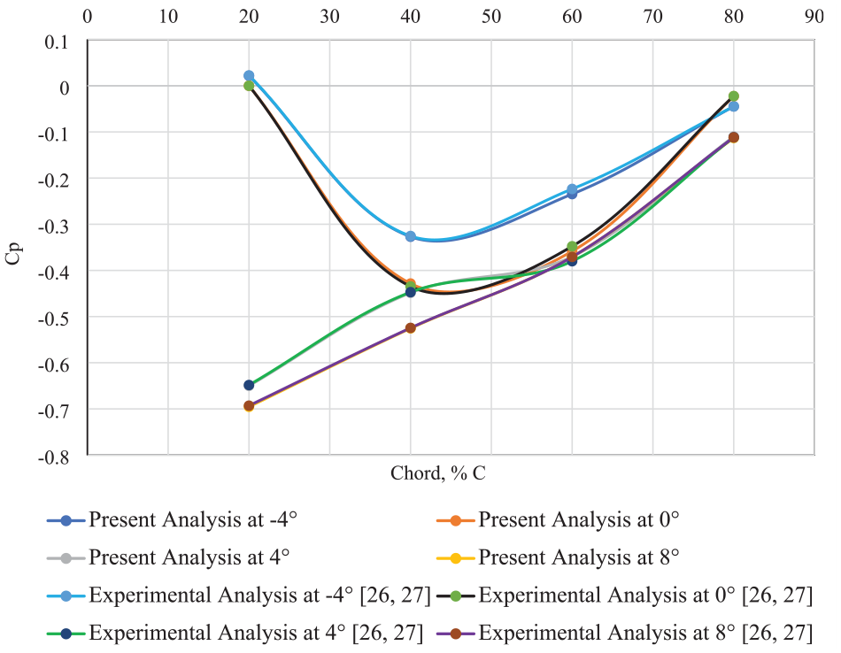
Pressure coefficient of upper surface at −4°, 0°, 4° and 8° AoA.

Figure 9.

Pressure coefficient of lower surface at −4°, 0°, 4° and 8° AoA.

It is observed from the figure that the pressure coefficient has maximum value of 0.025 at 20% of chord, while it has minimum value −0.36 at 45% of chord at −4° AoA. It is also observed that the pressure coefficient decreases initially from 20% up to 45% C and then rises gradually up to 80% C for the wing. Secondly, it has also minimum value −0.46 at 45% of chord at 0° AoA. It is observed that the pressure coefficient decreases initially from 20% up to 45% C and then rises gradually up to 80% C for the wing. Thirdly, it has minimum value −0.68 at 20% of chord at 4° AoA. It is observed that the pressure coefficient rises gradually up from 20% to 80% C for the wing. Finaly, it has minimum value −0.7 at 20% of chord at 8° AoA. It is also observed that the pressure coefficient rises gradually up from 20% to 80% C for the wing. It is also seen from the figure that the present numerical statistics of pressure coefficient for velocity of 30 m/s corresponds well with those obtained from experimental investigation.^26,27 This is encountered due to the orientation of airfoil’s upper surface.

In the figures, the violet, green, black, and orange colored line represents the simulation results of present analysis at −4°, 0°, 4° and 8° AoA.

It is observed from the figure that the pressure coefficient has maximum value of 0.057 at 80% of chord, while it has minimum value −0.146 at 20% of chord at −4° AoA. It is also observed that the pressure coefficient increases initially from 20% up to 45% C and then rises gradually up to 80% C for the wing. Secondly, the pressure coefficient has maximum value of 0.130 at 60% of chord while it has minimum value 0.05 at 20% of chord at 0° AoA. It is observed that the pressure coefficient increases initially from 20% up to 60% C and then decreases gradually up to 80% C for the wing. Thirdly, the pressure coefficient has maximum value of 0.046 at 80% of chord while it has minimum value −0.0246 at 20% of chord at 4° AoA. It is observed that the pressure coefficient rises gradually up from 20% to 80% C for the wing. Finaly, the pressure coefficient has maximum value of 0.096 at 20% of chord while it has minimum value 0.026 at 20% of chord at 8° AoA. It is also observed that the pressure coefficient decreases gradually up from 20% to 80% C for the wing. This is encountered due to the orientation of airfoil’s lower surface.

Pressure coefficient at 12°, 16°, 20° and 24° AOA

The pressure coefficient against the % of chord selected on the wings of the airfoil of wing with winglet at 12°, 16°, 20° and 24° AoA is demonstrated in Figures 10 and 11. In the Figure, the pressure coefficient represented by Cp is demonstrated in Y axis and % of chord is demonstrated in X axis. The present numerical statistics of pressure coefficient for velocity of 30 m/s is shown in the Figure, where the experimental results^26,27 of pressure coefficient for velocity of 30 m/s are also plotted in the Figure for the validation of present numerical statistics. In the figures, the blue colored line represents the simulation results of present analysis at 12°, the orange-colored line represents the simulation results of present analysis at 16°, the ash-colored line represents the simulation results of present analysis at 20°, the salmon-colored line represents the simulation results of present analysis at 24°, the red, green, black, purple represent the experimental results at 12°, 16°, 20° and 24° AoA.

Figure 10.

Pressure coefficient of upper surface at 12°, 16°, 20° and 24° AoA.

Figure 11.

Pressure coefficient of lower surface at 12°, 16°, 20° and 24° AoA.

It is observed from the figure that the pressure coefficient has maximum value of −0.1 at 80% of chord, while it has minimum value −0.72 at 20% of chord at 12° AoA. It is also observed that the pressure coefficient rises gradually up from 20% to 80% C for the wing. Secondly, the pressure coefficient has maximum value of −0.1 at 80% of chord, while it has minimum value −0.90 at 20% of chord at 16° AoA. It is also observed that the pressure coefficient rises gradually up from 20% to 80% C for the wing. Thirdly, the pressure coefficient has maximum value of −0.04 at 80% of chord, while it has minimum value −0.44 at 20% of chord at 20° AoA. It is also observed that the pressure coefficient rises gradually up from 20% to 80% C for the wing. Finaly, that the pressure coefficient has maximum value of 0.1 at 80% of chord, while it has minimum value −0.35 at 20% of chord at 24° AoA. It is also observed that the pressure coefficient rises gradually up from 20% to 80% C for the wing. It is also seen from the figure that the present numerical statistics of pressure coefficient for velocity of 30 m/s corresponds well with those obtained from experimental investigation.^26,27 This is encountered due to the orientation of airfoil’s upper surface.

In the figures, the blue, orange, ash, and yellow colored line represent the simulation results of present analysis at 12°, 16°, 20° and 24° AoA.

It is observed from the figure that the pressure coefficient has maximum value of 0.125 at 20% of chord, while it has minimum value 0.064 at 80% of chord at 12° AoA. It is also observed that the pressure coefficient decreases initially from 20% up to 40% C and then decreases gradually up to 80% C for the wing. Secondly, the pressure coefficient has maximum value of 0.164 at 20% of chord while it has minimum value 0.045 at 60% of chord at 16° AoA. It is observed that the pressure coefficient decreases initially from 20% up to 60% C and then decreases gradually up to 80% C for the wing. Thirdly, the pressure coefficient has maximum value of 0.0496 at 20% of chord while it has minimum value 0.074 at 40% of chord at 20° AoA. It is observed that the pressure coefficient decreases gradually up from 20% to 80% C for the wing. Finaly, the pressure coefficient has maximum value of 0.312 at 20% of chord while it has minimum value 0.125 at 80% of chord at 24° AoA. It is also observed that the pressure coefficient decreases gradually up from 20% to 80% C for the wing. This is encountered due to the orientation of airfoil’s lower surface.

Streamlines and velocity vector analysis near the airfoil surface

Streamlines and velocity vectors are essential tools in visualizing and understanding the aerodynamic behavior of the flow around the NACA 4418 airfoil. The direction and relative magnitude of airflow around the airfoil. Boundary layer characteristics, including laminar flow regions, separation points, and wake development. Areas of high velocity and low pressure that influence lift and drag generation.

Results at operational speeds

At the operational speed of 30 m/s, simulations were performed for various angles of attack (−4°, 0°, 4°, 8°, 12°, 16°, 20°, and 24°). Streamlines and velocity vectors around the airfoil reveal key flow features, which are summarized below:

At low angles of attack (−4° and 0°):

Streamline Behavior: The flow remains mostly attached, with smooth streamlines wrapping around the airfoil surface.

Velocity Field: High velocities are observed near the leading edge on the suction side, where the streamline curvature is greatest. The flow gradually decelerates as it moves towards the trailing edge.

Boundary Layer: Minimal separation is evident, resulting in low drag and moderate lift.

At moderae angles of attack (4° to 12°):

Streamline Behavior: Streamlines begin to diverge on the suction side due to increased pressure gradients. The flow accelerates along the leading edge, creating a significant velocity differential.

Velocity Vectors: On the suction side, velocity vectors indicate high-speed flow regions, while on the pressure side, velocities remain lower. Lift generation is maximized in this range of angles of attack.

Separation Zones: Slight flow separation may begin near the trailing edge, though it remains contained.

At high angles of attack (16° to 24°):

Streamline Behavior: Streamlines on the suction side show clear evidence of boundary layer separation and reversed flow, especially near the trailing edge.

Velocity Vectors: Near the leading edge, velocity vectors exhibit high magnitudes due to the steep angle of attack. However, separated flow dominates the rear portion, forming a wake region.

Flow Characteristics: Significant flow separation results in a substantial drag penalty and a reduction in effective lift.

Discussion

Lift and drag implications:

The attached flow at lower angles of attack promotes higher lift-to-drag ratios, as the velocity differential across the airfoil is optimized.

At higher angles of attack, the development of separated flow leads to a reduction in lift and a sharp increase in drag, marking the onset of stall conditions.

Pressure distribution correlation:

The streamline and velocity vector patterns align with the pressure coefficient distributions. High-speed flow regions correlate with areas of low pressure on the suction side, driving lift generation.

Conclusion

The computational analysis conducted in this study provides comprehensive insights into how winglets influence the aerodynamic behavior of NACA 4418 aircraft wings. The findings confirm that the presence of winglets causes a significant alteration in the pressure coefficient distribution, particularly at the wingtips. This change results in reduced vortex strength and, consequently, a decrease in induced drag, which contributes to improved aerodynamic efficiency.

The study validates that winglets can effectively enhance the lift-to-drag ratio, demonstrating their potential for optimizing aircraft performance by minimizing drag and enhancing lift characteristics. The results indicate that the pressure coefficient varies significantly based on the angle of attack and airfoil velocity, influencing the aerodynamic properties such as lift, drag, and overall efficiency. For example, at lower angles of attack (−4° and 0°), the pressure distribution exhibits a characteristic drop and rise pattern across the chord length, whereas, at higher angles (4° and above), the pressure distribution follows an increasing trend after an initial minimum. These observations are attributed to the airfoil’s surface orientation and the specific chord locations chosen.

The study’s outcomes emphasize the effectiveness of winglets in refining pressure distribution, thereby reducing undesirable aerodynamic phenomena like vortex formation. This contributes to the ongoing efforts in aerospace engineering to develop more fuel-efficient and high-performance aircraft through innovative wing design modifications. Future research should explore various winglet shapes, sizes, and orientations to further refine these aerodynamic benefits. Additionally, experimental validations of the computational models and an exploration of structural impacts due to winglet installations could provide a holistic understanding of the aerodynamic and operational implications of winglet configurations.

Future work

We recommend conducting additional studies to investigate the structural effects of installing winglets and to validate the computational models through experiments. Additionally, examinations explored the operational implications, such as changes in handling qualities and stall characteristics with varied.

Footnotes

Handling Editor: Sharmili Pandian

Declaration of conflicting interests

The author(s) declared no potential conflicts of interest with respect to the research, authorship, and/or publication of this article.

Funding

The author(s) received no financial support for the research, authorship, and/or publication of this article.

ORCID iD

Md. Abdullah

References

De Tullio

Xie

Chalke

, et al. Performance analysis of a heaving wing using DNS and LES. InDirect and Large-Eddy Simulation XI 2019; pp. 397–403. doi: 10.1007/978-3-030-04915-7_52

Choudhury

Cui

Motevalli

. Effects of Supercritical Airfoil Upper Camber Modification on Overall Airfoil Performance. MHMT 2020; ENFHT 227. doi: 10.11159/ENFHT20.02.

Lan

Meng

, et al. Aircraft design material-selection method based on MAUT theory. J Aeronaut Mater 2010; 3:88–94.

Lan

Guan

Jiao

, et al. A web-based computer-aided material-selection system for aircraft design. J Comp 2011. doi: 10.4304/JCP.6.5.976-983

Khabbaz

Manshadi

Abedian

, et al. A simplified fuzzy logic approach for material selection in mechanical engineering design. Mater Desig 2009; 30: 687–697.

Vio

Georgiou

Cooper

. Design of composite structures to improve the aeroelastic performance. In: 53rd AIAA/ASME/ASCE/AHS/ASC structures, structural dynamics and materials conference; April 2012; p. 1458.

Sivaraj

Ishak

Nasirudin

, et al. Investigation of aerodynamic characteristics of a wing model with RGV winglet. 2021. doi: 10.6084/m9.figshare.14291385.

Sethunathan

Ramasamy

. Aerodynamic performance characteristics of winglet configurations for the low and medium Reynolds number operations. Int J Mod Phys C. 2023. doi: 10.1142/s0129183123501218

Flores-Mezarina

Bravo-Mosquera

Garcia-Ribeiro

, et al. Application of wavy leading edge to enhance winglet aerodynamic performance. J Roy Aeron Soc. 2023. doi: 10.1017/aer.2022.97

10.

Cheruthuruthy

Prakash

. Computational fluid dynamics study of aircraft wing with winglet performance at high subsonic speeds. Int Rev Aerosp Eng 2022. doi: 10.15866/irease. v15i5.22870

11.

Wang

Ding

Han

, et al. Parametric study on thermo-hydraulic performance of NACA airfoil fin PCHEs channels. Energies. 2022. doi: 10.3390/en15145095

12.

Suryolaksono

Bramantya

. Numerical simulation of the effect of NACA 0012 nozzle geometry on ducted propeller performance. Proc Eng Life Sci 2023; 4.

13.

Gkiolas

Mathioulakis

. Aerodynamic Study of a NACA 64418 rectangular wing under forced pitching motions. Fluids. 2021. doi: 10.3390/FLUIDS6110394

14.

Hariyadi

. An analysis on aerodynamics performance simulation of NACA 23018 airfoil wings on cant angles. 2017. doi: 10.22219/JEMMME.V2I1.4905

15.

Marino

Watkins

Sabatini

, et al. Unsteady pressure measurements on a MAV wing for the design of a turbulence mitigation system. 2014. doi: 10.1109/METROAEROSPACE.2014.6865909

16.

Ismail

Kaisan

Balogun

, et al. Effect of angle of attack on lift, drag, pitching moment and pressure distribution of NACA 4415 wing. J Sci Technol Edu 2020; 8(1): 31–44.

17.

Liu

, et al. Predicting pressure coefficients of wing surface based on the transfer of spatial dependency. AIP Adv. 2022. doi: 10.1063/5.0093144

18.

Chen

Cheng

Tian

. Research on the pressure distribution under different airfoil types of aircraft. J Phys 2023. doi: 10.1088/1742-6596/2441/1/012005

19.

Bakhai

Mat

Musa

NAA

. Aerodynamics of a wing body with different Winglet Can’t Angle. In: E3S Web of Conferences; 2023. doi: 10.1051/e3sconf/202447700029

20.

Vaishak

Reddy

Shali

. Aerodynamic analysis of supercritical airfoil. 2021. doi: 10.1063/5.0057918

21.

Patel

Mankar

Kadam

, et al. Aerodynamic analysis of variable Cant Angle Winglets for Higher Mach regimes. Int J Eng Technol Manage Sci 2023. doi: 10.46647/ijetms. 2023.v07i01.001

22.

Nguyen

Pham

. Aerodynamic analysis of aircraft wing. VNU J Sci Math-Phys 2015; 31.

23.

Abdelghany

Sarhan

Alahmadi

, et al. Study the effect of winglet height length on the aerodynamic performance of horizontal axis wind turbines using computational investigation. Energies 2023; 16: 5138.

24.

Farghaly

Abdelghany

. Study the effect of trailing edge flap deflection on horizontal axis wind turbine performance using computational investigation. Int J Renew Energy Res 2022; 12:1942–1953.

25.

Raj

Rose

. Influence of bioinspired morphing on the flow field characteristics of UAV wings at low Reynolds number. Proc Instit Mech Eng, Part G: J Aerosp Eng 2024; 238: 1503–1533.

26.

Ara

Ali

Islam

Akhter

. An experimental investigation on the aerodynamic characteristics of NACA 4412 with winglets. 2019; 2121: 060004.

27.

Ara

Ali

Islam

, et al. Performance study of winglets on tapered wing with curved trailing edge. 2017; 1851: 020005. doi: 10.1063/1.4984634

Computational assessment of winglet-induced variations in pressure coefficients on NACA 4418 aircraft wings

Abstract

Keywords

Introduction

Method of numerals

Airfoil geometrical parameters

Meshing

Boundary conditions

Residual display

Solver edition

Simulation techniques

Geometry andmeshing

Boundary Conditions

Turbulence model

Solver settings

Residual and Convergence

Validation and post-processing

Grid sensitivity analysis

Results and discussion

Pressure Coefficient at −4°, 0°, 4° and 8° AOA

Pressure coefficient at 12°, 16°, 20° and 24° AOA

Streamlines and velocity vector analysis near the airfoil surface

Results at operational speeds

Discussion

Conclusion

Future work

Footnotes

Declaration of conflicting interests

Funding

ORCID iD

References