Abstract
Decarbonisation of domestic heating in the UK is expected to involve widespread replacement of gas boilers with heat pumps. This transition requires a reduction in heating system flow temperature for the heat pump to operate efficiently, which can necessitate costly radiator or fabric upgrades to provide sufficient heat. The requirements for existing dwelling and heating systems to have these upgrades therefore directly impacts the “heat pump readiness” of the UK stock. This paper applies a novel approach in using diagnostic data for approximately 4600 boilers to evaluate the viability of installing heat pumps with no changes made to the existing radiators or fabric. Results indicate that 31% of dwellings in the sample could operate with Low Temperature Heat Pumps (LTHPs) without upgrades to radiators or fabric, or up to two thirds with High Temperature Heat Pumps (HTHPs), whereas previous analysis using surveys has found that radiator upgrades are almost always needed. Therefore, the costs and disruption of heat pump roll out could be substantially lower than previously predicted, and the use of real heating system performance data could supplement survey-based assessments of heat pump readiness to help identify more accurately where upgrades are needed.
Practical application
Current design practices almost always lead to replacement of existing radiators when switching a gas boiler for a heat pump. However, analysis of diagnostic data from approximately 4600 boilers in the UK suggests this may not be entirely necessary. This measured heating system data indicates that up to two-thirds of UK dwellings could operate with High Temperature Heat Pumps (HTHPs) without upgrading existing radiators. Henceforth, development of data-driven testing procedures for the design of future heating systems has significant potential to facilitate rapid heat pump deployment at a national scale, a crucial step in decarbonising buildings in the UK.
Introduction
Replacement of gas boilers with heat pumps is expected to play a key role in decarbonising domestic heating in the UK, as part of its commitment to achieving net zero carbon emissions by 2050. 1 Ambitious installation targets (600,000 pa by 2028) mean that streamlining the heat pump installation process in retrofit and better estimating the viability and cost of installations is of key importance.
When replacing a gas boiler with a heat pump, conversion to a low temperature heating system is often necessary. This conversion involves lowering the temperature of the water supplied by the heating plant, known as the flow temperature, in hydronic heating systems. Although high temperature heat pumps are available, the efficiency of all heat pumps drops with higher flow temperatures. Therefore, to minimise running costs (in the face of the large gas: electricity price gap), carbon emissions, and the need for expensive grid reinforcement work, lower flow temperatures are desirable. The necessary change in flow temperature is often significant, moving from flow temperatures of 60-70°C typical for boilers to temperatures ideally lower than 45°C with a heat pump. 2
Reducing the flow temperature will result in radiators emitting less heat, hence the conversion to lower flow temperatures can require changes to provide sufficient heating. These changes may include replacement of radiators with larger ones that emit more heat, upgrades to the building fabric to reduce heat demand, and running the heating system more continuously to spread out the heat load. Upgrading existing radiators is common practice when replacing a boiler with a heat pump in the UK as it is often the more cost-effective option but can still incur significant costs. For example, full replacement of a dwellings existing emitter network is estimated to cost up to £6000-£7500. 3 This would result in full heat pump installation costs exceeding the £7500 grant offered by the UK’s Boiler Upgrade Scheme. Besides costs, replacing radiators also adds disruption to heat pump installation, with additional time required in installation.
The additional costs and disruption associated with replacing radiators means that understanding the extent to which this is required directly impacts the speed and extent of widespread roll out of heat pumps in the UK. A study by BEIS 2 aimed to understand this further by characterising the readiness of 515 existing heat distribution systems to operate at lower flow temperatures, as the state of existing systems in the UK was broadly unknown. The study involved surveying the dwellings, estimating building heat loss, and installed radiator output at a variety of flow temperatures, where total radiator output needs to exceed the peak heat loss to provide sufficient heating. Results indicated that although most heat distribution systems were oversized for existing boiler flow temperatures, they would most often be undersized for typical heat pump flow temperatures. For example, the results indicated that 90% of UK dwellings would require new radiators to meet peak heat load for a common maximum heat pump flow temperature of 55°C or 99% at 45°C. Furthermore, when considering the possibility of radiator performance degradation and underestimation of building heat loss by the surveys, the proportion of heating systems requiring radiator upgrades for common heat pump flow temperatures approaches 100%. Moreover, similar surveys to that used in this study, such as the MCS heat loss survey, are used to assess whether radiators should be replaced when designing heat pump heating systems in the UK. Thus, in both the development of heat decarbonisation scenarios, and the actual installation of heat pump systems in the UK, it is generally assumed that radiator upgrades are needed, significantly adding to the costs and disruption associated with heat pump roll-out.
Although this survey-based approach has provided useful insight, an assessment of existing systems’ suitability with heat pumps using measured data on the performance of heating systems has not been made. Empirical analysis is advantageous, as predicting the required capacities of radiators using surveys carries uncertainties which can be partially addressed using measured data. Primarily, surveys estimation of peak heat loss and subsequent required heat load is frequently reported to be different to that measured4–6 and has resulted in growing interest for incorporating measured performance data into the models and decisions for retrofit. 7 Further, radiator outputs are estimated using manufacturer values tested according to BS EN 442 8 and may not be representative of performance for real installations, 2 due to a potential build up of sludge, air, or poor hydraulic balancing. This uncertainty was acknowledged in BEIS, 2 with a sensitivity applied to investigate the effect of the average reported uncertainties in the surveys. Conversely, the primary advantage of using measured data, which captures heat delivered by a heating system and the flow temperatures required to do so, is that it intrinsically encompasses real performance of the heating system and the heat demand as set by the occupants, overcoming these uncertainties and capturing the variability of real performance.
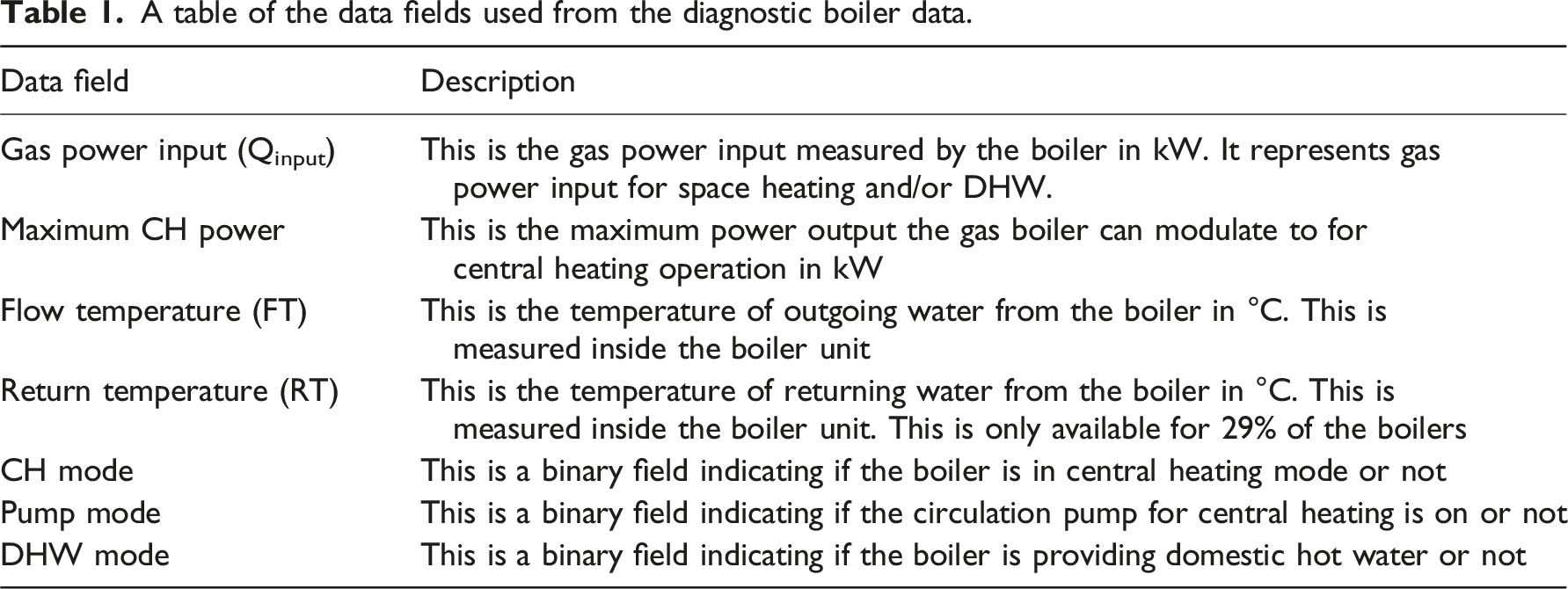
A table of the data fields used from the diagnostic boiler data.
Furthermore, the measured flow temperature of the boilers is considered indicative of the installed radiator capacity because radiator output is dependent on the temperature difference between the water in radiators and the air in rooms, with flow temperatures making up most of the variation in this temperature difference. Thus, the data has potential to show the flow temperatures necessary to meet peak heat demand, which can suggest if existing radiators can meet peak heat demand with heat pumps. Moreover, the peak heat demand for each boiler can be extracted, to show if typical maximum outputs for domestic heat pumps can meet this, showing whether fabric upgrades are necessary before installing a heat pump. Furthermore, the yearly heat demand of boilers, estimated by their sum gas power input between August 2021 - August 2022, follows a similar (but not identical) distribution to that modelled by the National Housing Model (NHM), shown in Figure 1. This indicates that heat demand across the sample is not atypical for boiler heated dwellings across the UK, whereby it is assumed in this study that the dataset can be used to approximate UK gas heated dwellings as a whole. Therefore, this research aims to address the question: for a like for like heat demand, what proportion of UK dwellings with boilers can have a heat pump installed with no changes made to the existing radiators or fabric? Comparison between annual gas power input of boilers in this dataset and annual space heating demand for gas heated dwellings in the National Housing Model (NHM). This version of the NHM uses English Housing Survey (EHS) data and multiple years of gas metering data from the National Energy Efficiency Data-Framework (NEED) to estimate gas heat demand across the UK housing stock.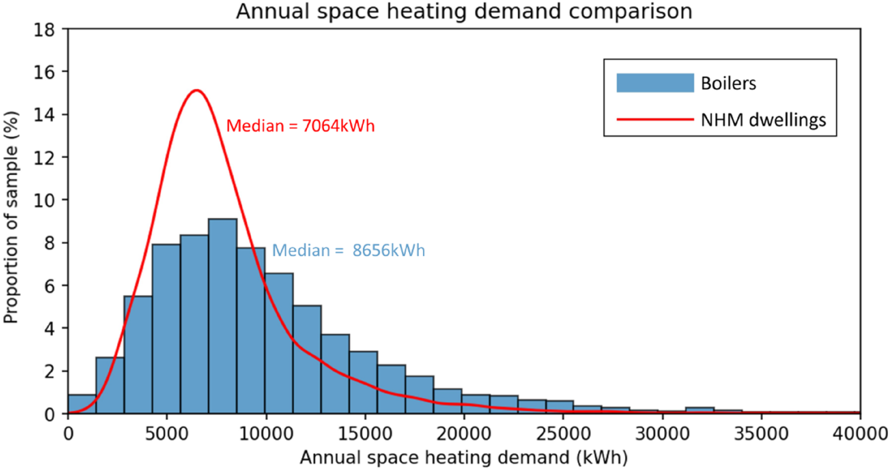
Data and methods
In this dataset, simply looking for maximum flow temperatures does not indicate the required flow temperature to meet peak heat demand, due to on-off boiler cycling and the intermittency in heating operation. Measured flow temperatures would only be indicative of what is required to meet heat demand with existing radiators if the boiler was exactly matching the required heat load with continuous heating in steady state. Rather, during heating periods, boilers will tend to cycle on and off. This is firstly due to the setting of flow temperature set points without weather compensation for the boilers in this dataset, and secondly because combi boilers are not sized to provide space heating in steady state, even when maintaining a steady internal temperature for the dwelling. Instead, combi boilers are often sized for domestic hot water demand, which can be significantly greater than that for space heating, leading to cycling due to the minimum modulation ratio of boilers.
10
Furthermore, the heating system will only call for heat according to heating schedules, which adds more transience to heating operation, requiring additional heat to warm the heating system and dwelling from cold when the heating has been off for extended periods of time. Additionally, not all the gas power input is for space heating, and domestic hot water (DHW) events have simply been removed to reduce interaction between space heating and DHW demand. An example time series from a boiler in the dataset is provided in Figure 2, illustrating on-off boiler cycling and interaction with hot water events. An example time series plot from one of the boilers in this dataset. Flow temperature and return temperature are plotted at the top, the gas power input profile is plotted in the middle, and control information on the boiler mode is plotted at the bottom – including central heating, domestic hot water and active circulation pump modes. Return temperature data is only available for 29% of the boilers in this dataset.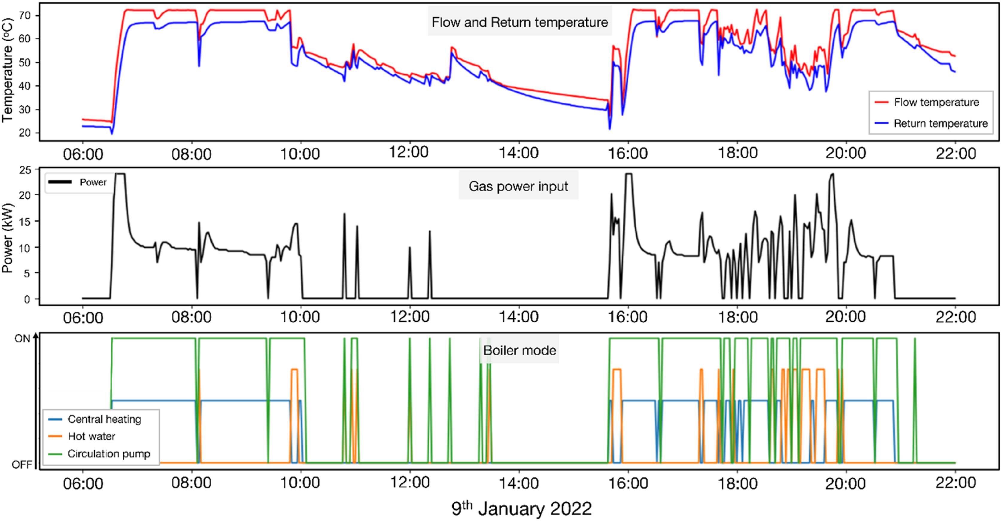
Flow temperature data
The intermittent operation of boilers presents several obstacles to direct analysis of flow temperature data. Firstly, when the heating system is off, and radiators cool to room temperature, the heat transfer characteristics of the radiators are likely to change as water is no longer flowing. Moreover, flow temperatures in this dataset are only meaningful when the pump is running, known from the control data. This is because the flow temperature sensor is inside the boiler and will measure an insulated plug of water when the pump is not running. Hence, the flow temperature in these periods will not be representing radiator capacity in hydronic operation. Therefore, averaging flow temperatures over time will not be indicative of the temperature required to meet heat demand with steady state heating, and a more sophisticated method of analysing the flow temperature data was needed.
Instead, to estimate the minimum required flow temperature for a given heating period, it was necessary to use the power profiles of boiler operation. Specifically, it was assumed in this study that the power profiles could be averaged over time to estimate the underlying heat demand, which would represent the heat load required for continuous steady state heating. The change in heating power from in situ heating when the gas boiler is on, to continuous heating required to meet the underlying heat demand, was used with a theoretical power-flow temperature relationship to correct in situ heating flow temperatures to that required for steady state heating (see Estimating flow temperature required).
Power data
Before power profiles could be used to estimate the underlying heat demand required for continuous heating, it was necessary to consider the dynamics of the heating system, whereby heat storage and release make simple energy balancing over short time periods impractical. For example, when the heating system is heated from cold, additional heat will be required to raise its temperature, dependent on the temperature rise and the thermal mass of the heating system. Because the power input measurement from the boiler only represents the heat that has gone into the heating system, rather than the output from the heating system to the dwelling, power input measurements during warming up periods will overestimate heat output to the dwelling. Furthermore, when the heating is turned off, there is no power input from the boiler, but the radiators will still emit heat as they cool down towards room temperature, which needs to be accounted for to estimate underlying heat demand. This phenomenon can be represented in Equation (1), where there are two components to the power input into a heating system (Qinput), the heat that has been transferred to (or out of) the heating systems thermal mass (Qcharge) and the heat that has been transferred from the heating system to the dwelling (Qoutput). Equation (2) shows that Qcharge is a function of the heating systems thermal mass (CHS) and the rate of change of heating system temperature (THS), where the temperature of the heating system is often approximated as the arithmetic mean between flow (TF) and return (TR) temperatures (see Equation 3). Further, Equation (2) shows that Qoutput depends on the mass flow rate (m), specific heat capacity of the fluid (c), and the heating system temperature drop (TF-TR). Estimating either Qcharge or Qoutput can allow for disaggregation of the two in measured Qinput, however, because the flow rate in the heating system is unknown, estimation of Qcharge was preferrable, and involved developing a method to estimate thermal mass. This allows for an estimate of heat transfer to the dwelling to be calculated, so that underlying heat demand can be approximated.
Estimating heating system thermal mass and underlying heat demand
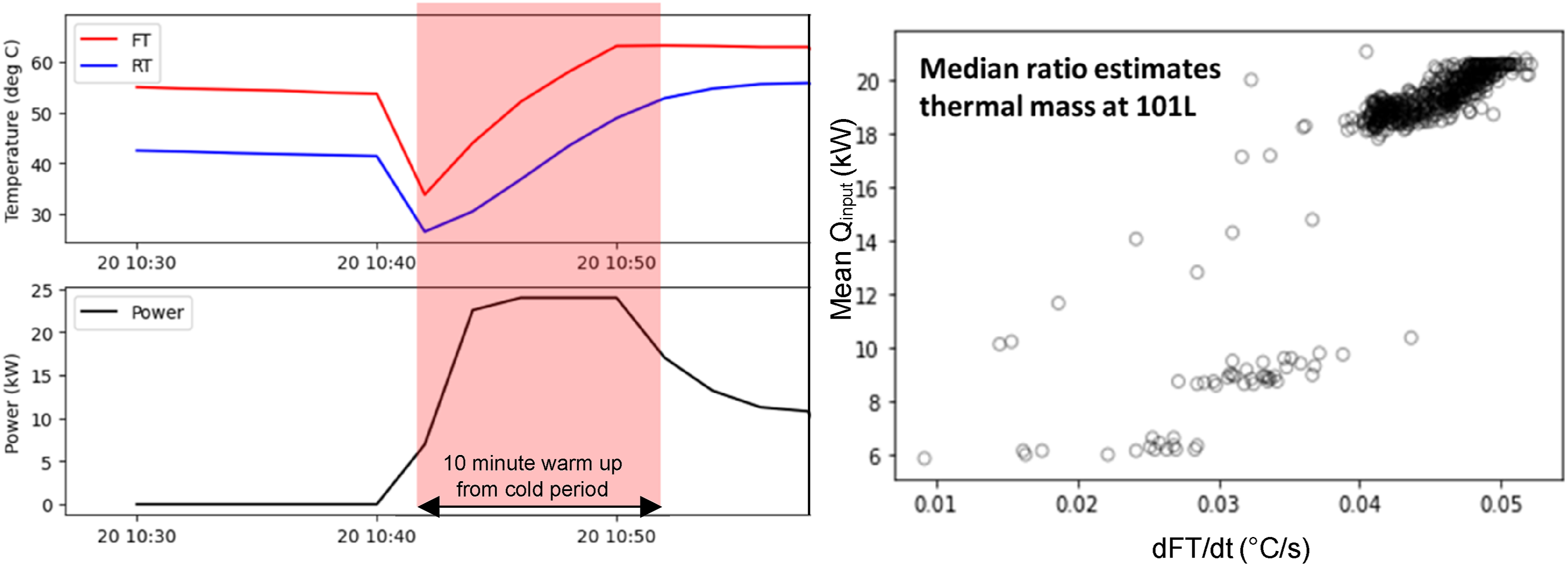
The thermal mass of each heating system in the dataset has been estimated by isolating warm up from cold periods. Specifically, these have been defined as the first 10 minutes of heating when the flow temperature at the start of a heating period is 35°C or less. An example of one of these warm up from cold periods is demonstrated in Figure 3 showing the rapid increase in flow temperature and high power input required to charge the thermal mass of the heating system. The average power input and water temperature rise during this period can be used to approximate the thermal mass of the heating system, by using Equation (4). This is a simplification, likely leading to thermal mass being an overestimate, as there will be some heat output to the dwelling in this period, but the heat charging the thermal mass should be dominant. Specifically, flow temperature (TF) is used instead of mean water temperature (THS), as return temperature (TR) data was not commonly available. For each warm up from cold period, a thermal mass value is estimated, and the median of these values is used to estimate the thermal mass of the heating system. An example of this process is demonstrated in Figure 3, showing the scatter between average power input and rate of change of flow temperature in each warm up from cold period. There is clear clustering, indicating approximation of the heating systems thermal mass (including the water, pipes and radiators). An example of a warmup from cold period for one of the boilers is shown on the left, with flow (FT) and return (RT) temperature plotted at the top and the gas power input plotted at the bottom. On the right, a scatter plot between boiler heat input and rate of change of flow temperature for each warmup from cold period is displayed, with the median ratio between the two variables displayed as the estimate of the heating systems thermal mass in litres of water equivalent.
Power output from the heating system to the dwelling could then be approximated. Primarily this was done by estimating the heat that has gone into charging (or discharging) the thermal mass of the heating system, calculated by the rate of change of flow temperature multiplied by the estimated thermal mass, as seen in Equation (2). This can then be subtracted from the power input measured by the boiler to approximate heat output from the heating system. This also enables estimates of heat output during radiator cooling, based on falling temperature. However, because flow temperatures only measure an insulated plug of water when the pump is off, heating system temperatures need to be modelled during cooling periods. This has been done by interpolation of flow temperatures between periods when the pump is off, a simplification which assumes a constant rate of cooling. Physically sensible rules were also applied, firstly, heat input charging the heating systems thermal mass could not exceed the power input by the boiler in that interval. Secondly, power output during radiator cooling could not exceed the maximum central heating power output of the boiler. And thirdly, the energy stored in the heating system was counted so that heat output during cooling could only use stored heat, ensuring the calculation was energy balanced. Finally, the calculated heating system power output was used to estimate underlying heat demand, by averaging it over time.
Estimating flow temperature required
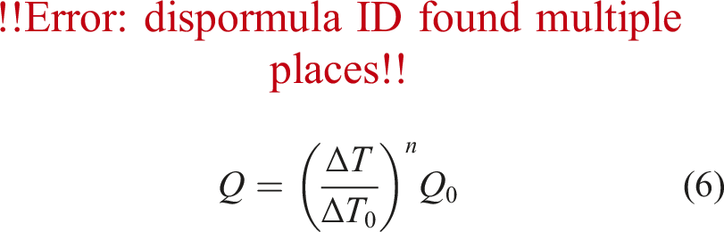
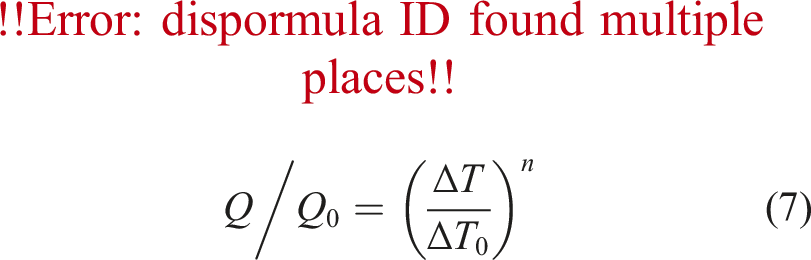
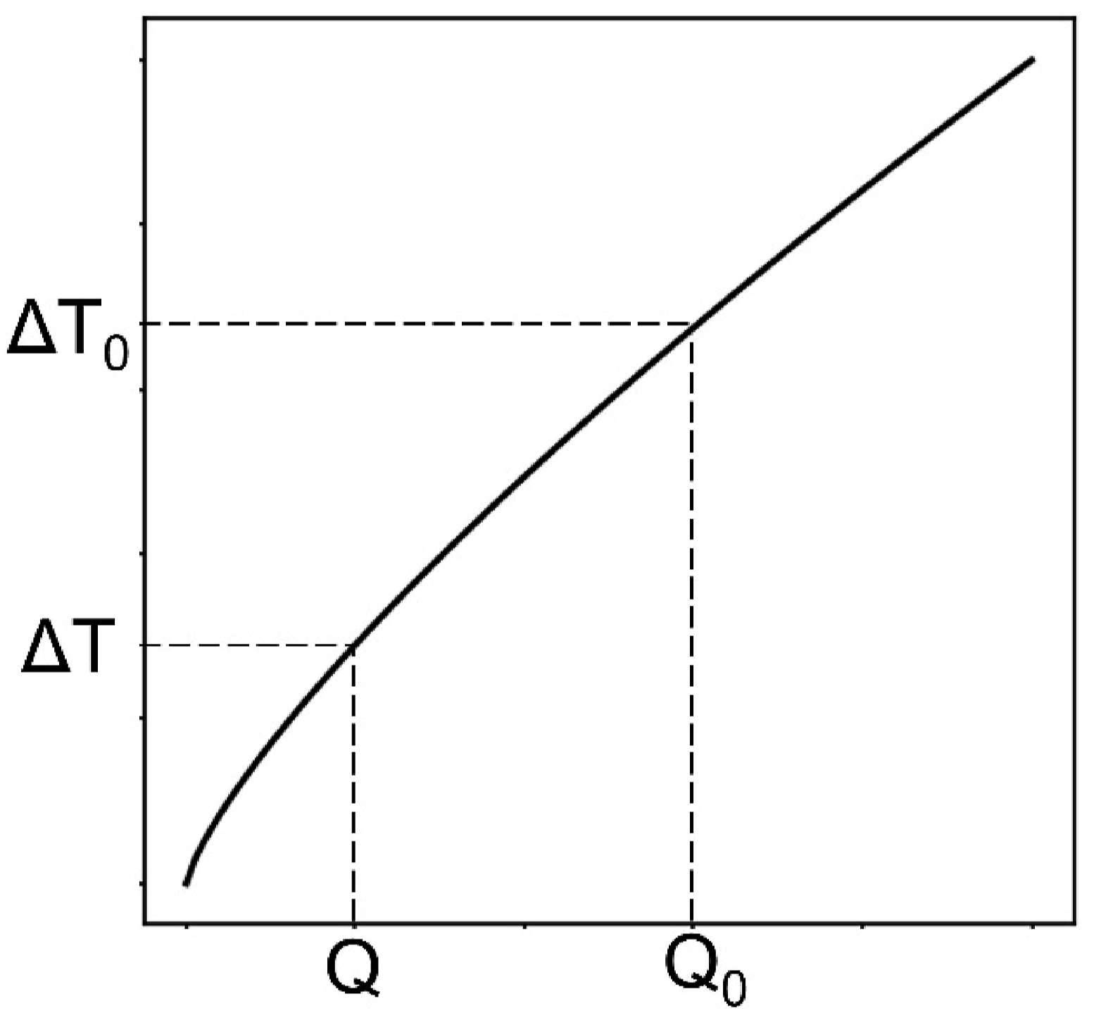
Estimated underlying heat demand could then be used to estimate the flow temperatures required to meet this with steady state heating, which when taken over all heating periods in the heating season, approximated the maximum flow temperature required to meet peak heat demand. To calculate required flow temperature, the theoretical relationship between radiator power output and flow temperature was needed. This is shown in Equation (7) and Figure 4 where radiator power output decreases as the temperature difference (ΔT) between water temperature (THS) and room decreases (TI) . Specifically, this is not linear, and follows a power law according to the n-exponent, typically at a value of 1.3 for panel radiators, representing the temperature difference dependent contribution of radiation and convection. The ratio between underlying heat demand and heat output for in situ heating from the boiler was used to “correct” the flow temperatures measured during the in situ heating phases. Specifically, in situ heating involved periods when the boiler was in central heating mode, and the estimated power output exceeded 1 kW, preventing selection of transient flow temperatures. Because the internal temperature of the dwellings was not known, and nor was the temperature drop across the heating system (in most cases), these temperatures needed to be assumed in Equation (7). In a baseline case, an internal temperature of 20°C was used, and a temperature drop across the heating system of 8°C was used, derived from the average temperature drop measured for boilers with return temperature data (Figures 10 and 11, appendix). These parameters were varied to estimate model sensitivity, discussed in Assumptions of internal temperatures and flow-return temperature difference. By iterating this process for an averaging window across the whole heating season, the maximum required flow temperature out of all these averaging periods represents the flow temperature required to meet occupant heat demand with continuous heating. In other words, this can show if peak heat demand can be met at flow temperatures heat pumps can provide, thus indicating whether existing radiators need to be replaced or not. Furthermore, the maximum estimated power output across all averaging intervals will represent the peak heat demand for the dwelling and is extracted to assess if common heat pump capacities can meet heat demand, or if fabric upgrades are required. The non-linear relationship between excess temperature and power output of radiators, plotted for an n-exponent of 1.3.
Deciding the averaging window to estimate underlying heat demand in this method is important, as it will impact the scheduling and rate of heat delivery for the calculated underlying heat demand. The choice of length is a compromise between removing boiler specific on-off cycling, which does not need to be replicated with heat pumps, and avoiding large changes in occupant heating schedules, which could substantially affect dwelling heat loss. If the averaging window is too long, for example, an entire day, then the heat load required for continuous heating could underestimate heat required on smaller timescales, particularly as heat loss in a building changes over the course of a day, and the overall heat demand will be higher due to a higher average internal temperature from continuous heating. On the other hand, if the averaging window is too short, it may fail to approximate steady state heating and smooth out boiler on-off cycling. A window of 30 minutes was sufficient to smooth intermittency in Watson & Bennett. 9 In this analysis, averaging windows of six, three, and 1 hour were used. Six hours was considered an appropriate maximum averaging window to capture the more continuous heating profiles typically used by heat pumps, 13 with sufficiently low heat loss variation in this period that it will not significantly impact the ability to deliver sufficient heat. However, it will effectively change scheduling, for example, the heating may turn on up to 3 hours earlier, more gradually heating the dwelling. Contrarily, 1 hour averaging aims to capture the heat load required with minimum changes to scheduling but may be more intermittent than most heat pump heating profiles. The averaging window applied is a moving window, rather than starting and finishing at fixed times. This avoids any anomalous results that might occur purely due to the choice of starting and finishing time.
Categorising heat pump readiness
When running the model, data compiled on each boiler included: the maximum required flow temperature, the percent of heating periods that could be met at 55°C, the maximum heat demand, and the estimated thermal mass value. After removing any data with more than 5% missing values, the final sample size was 4594 boilers.
A table describing the different heat pump readiness categories and parameters.
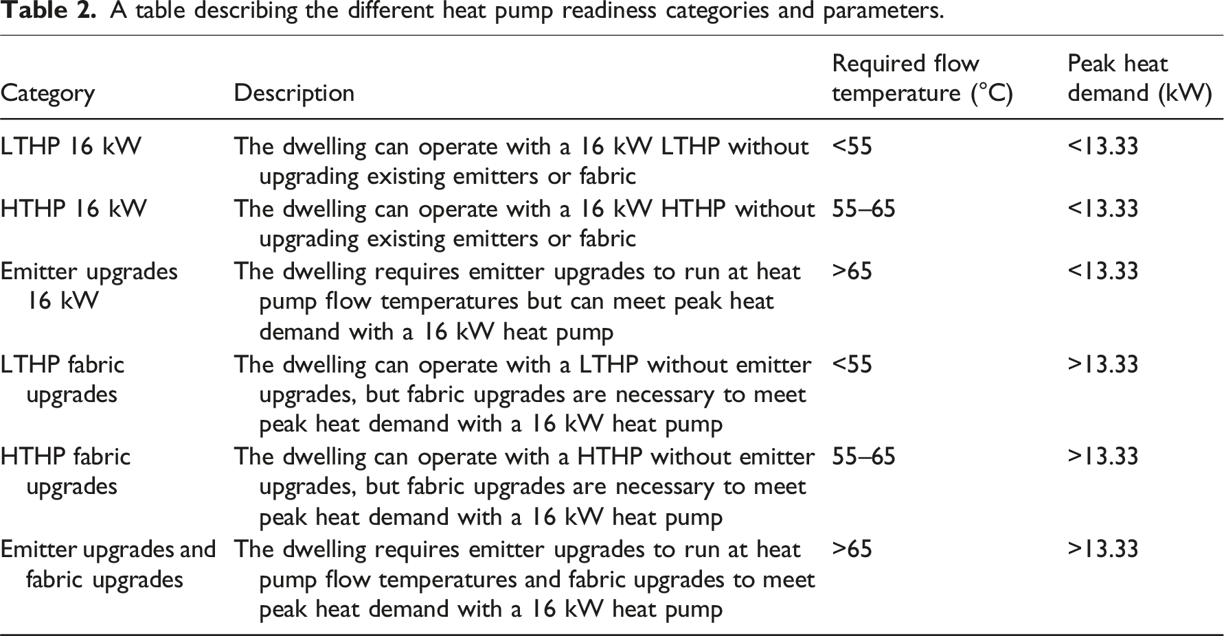
Selected flow temperature boundaries are based on common design flow temperature criteria, which radiators will be sized to, rather than the maximum possible flow temperatures of individual heat pumps. 14 For peak heat demand, a 16 kW heat pump was selected as the maximum capacity of domestic ASHPs readily available on UK markets. 3 To assess if peak heat demand could be met with a 16 kW heat pump, a 20% intermittency factor was applied, as is best practice in MCS heat pump sizing guidance 15 to account for heating time necessary with intermitted heating profiles, so the highest peak heat demand that could be met with a 16 kW heat pump is 13.33 kW. Technically, the effects of intermittency should be partially accounted for, as the averaging windows used do not fully smooth occupant heating schedules. However, additional factors may make the 20% factor useful, for example rated heat pump outputs can be lower in peak winter conditions.
Summary of method
The full method used to estimate required flow temperature, peak heat demand, and resulting heat pump readiness is summarised in Figure 5. A flow chart demonstrating the key steps in the method.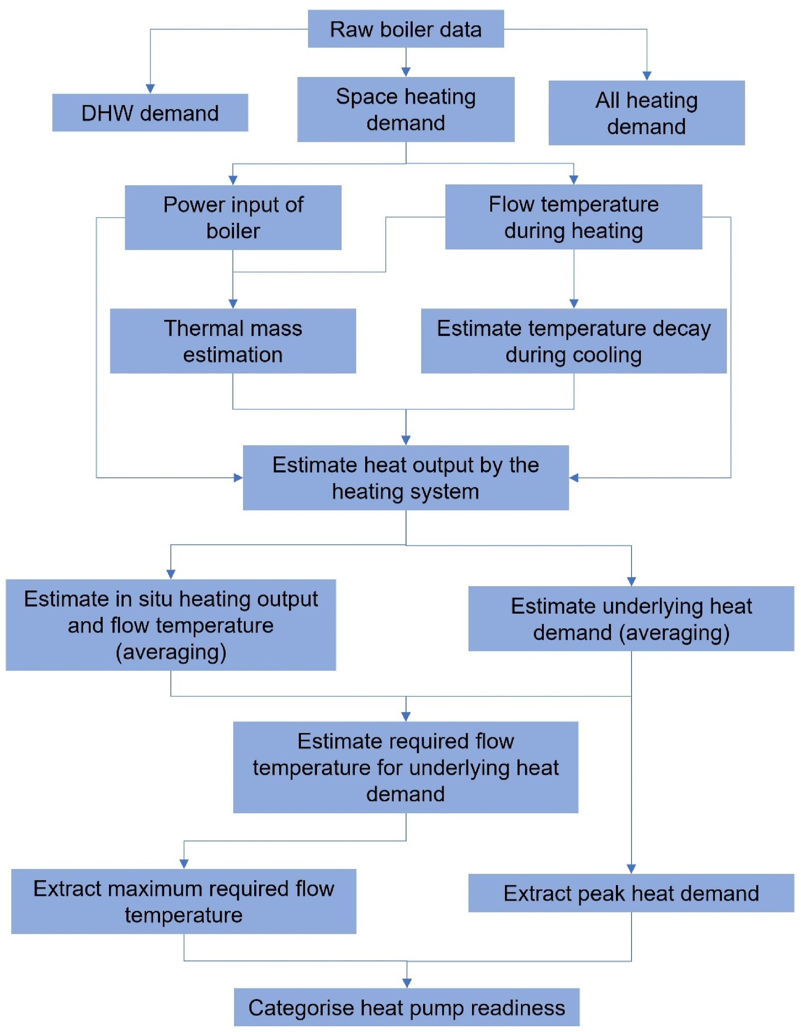
Results
Figure 6 displays the baseline case results for six hourly averaging of heat demand. Six hours was chosen as representative of the common industry advice to run HPs in a near continuous manner through extension of the heating period. It appears to show more dwellings could operate at heat pump flow temperatures without making changes to their existing radiators than previous research suggested.
2
The distribution of maximum required flow temperatures also approximates a normal distribution, like the distribution in radiator oversizing seen in BEIS,
2
but shifted, to suggest lower flow temperatures are possible. For example, the model estimates that 31% of dwellings could operate with a 16 kW or smaller capacity LTHP with no changes made to existing radiators. This contrasts to 10% of dwellings predicted to require no radiator upgrades at 55°C or lower flow temperatures in a similar estimate made using surveys in BEIS,
2
of which, this number approximated 0% when accounting for survey uncertainties. Furthermore, the model estimates that 28.7% of dwellings require radiator upgrades to meet heat demand with HTHP or LTHP flow temperatures, compared to 54% estimated in BEIS.
2
Additionally, the model also estimates that approximately 10% of dwellings will require fabric upgrades to meet peak heat demand with a 16 kW heat pump. The primary results for 6-h averaging of heat demand, showing a scatter plot between maximum heat demand and maximum required flow temperature for each boiler analysed (N = 4594). Accompanying histograms of each axis are provided. Furthermore, the results are segmented into the six heat pump readiness categories, with proportions displayed.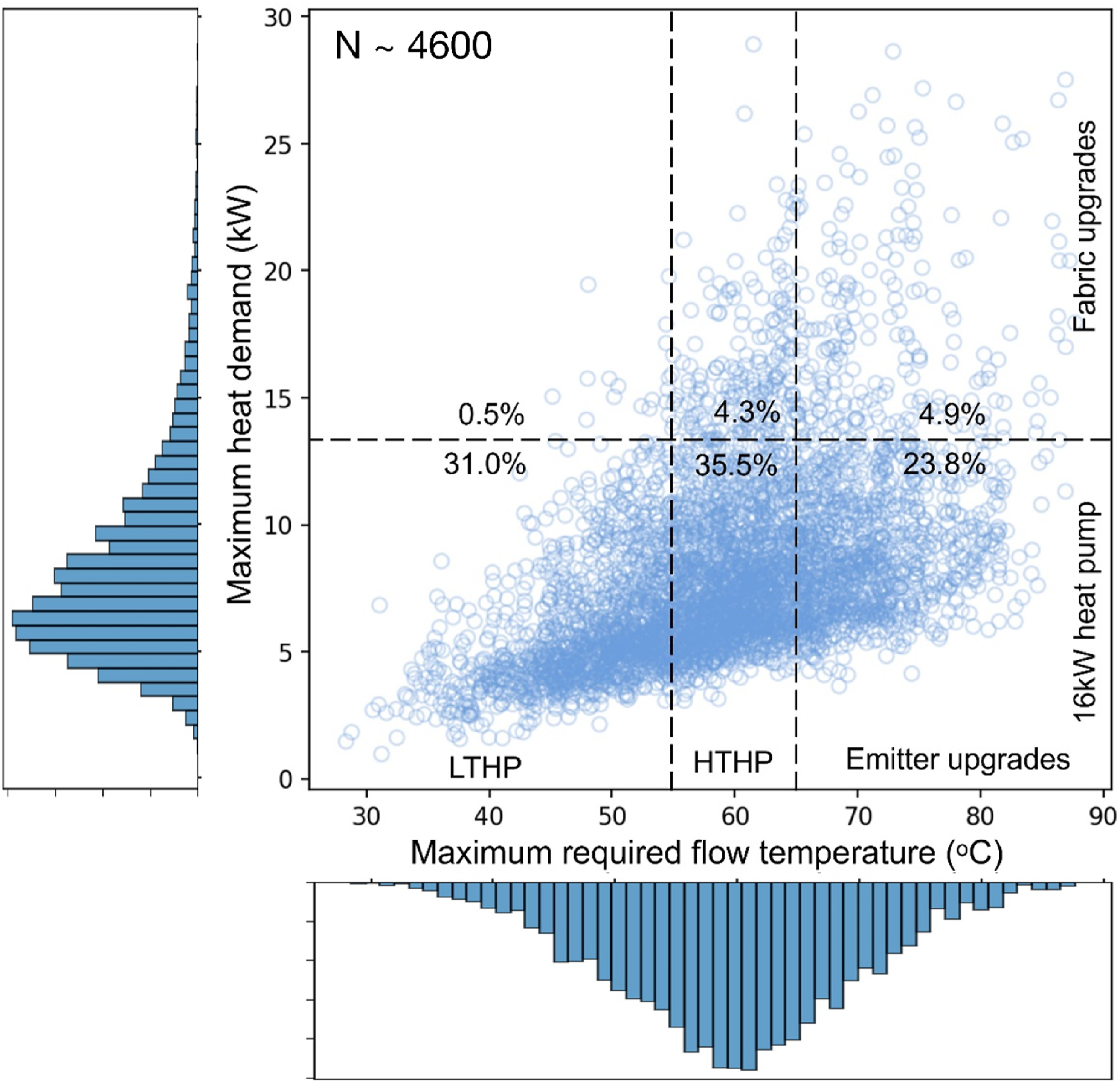
In Figure 7, the proportions of dwellings falling into the six categories of flow temperature and heat demand requirements are shown for each time averaging window applied, six, three, and one hourly. The results are expected, with lower time averaging of heat demand resulting in higher peak heat demands requiring higher flow temperatures to provide sufficient heat. For example, for 1 hour averaging, only 6.7% of dwellings could meet peak heat demand with a 16 kW LTHP, and 17.8% with a 16 kW HTHP. However, this shows that even with minimum changes to heat scheduling, which is unusual in typical heat pump designs, some dwellings can already operate at heat pump flow temperatures, particularly when considering high temperature heat pumps. Moreover, these results also demonstrate the usefulness in spreading out the heat load when switching from a boiler to a heat pump. For example, 1 hour averaging results estimate that 26.7% of dwellings will require both emitter and fabric upgrades to meet heat demand, compared to just 4.9% when averaging the heat load over 6 hours. The 1 hour averaging results also demonstrate the potential for existing boiler heating systems to lower their flow temperatures, without adaptation of the heating schedule, which will improve existing heating systems efficiency, and has been observed in emerging research.
16
A bar chart showing the proportion of dwellings (N = 4594) in each heat pump readiness category for the different levels of heat demand averaging applied, six, three, and one hourly (6H, 3H, 1H). EU and FU stand for emitter upgrades and fabric upgrades respectively. The error bars represent the upper and lower bound uncertainty modelled from the internal temperature and heating system temperature drop sensitivity.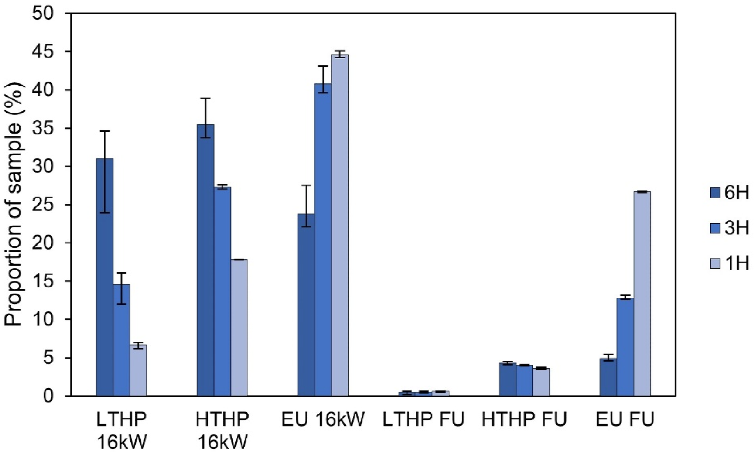
Additionally, in Figure 8, the proportion of dwellings that could operate at 55°C or lower for different proportions of the heating season are shown for each heat demand time averaging window modelled. This includes 100, 99, 95, and 90% levels, where 90% would mean 90% of required flow temperatures in the heating season were at or below 55°C. Generally, the figure demonstrates that the maximum required flow temperature is only needed for a very small period, where even going from 100% to 99% of the heating season makes a significant difference. For example, for six hourly averaging, 31.5% of dwellings could meet peak heat demand at 55°C for the entire heating season, but 52.6% of those dwellings could operate at 55°C or lower for 99% of the heating season (where 1% is equivalent to approximately 2 days of time for an October to April heating season). The results raise the potential benefits of small amounts of system hybridisation, for example, with supplementary electric heaters, or boilers (gas or hydrogen), to help in meeting peak heat demand. This could ease the requirements of emitter and fabric upgrades when installing heat pumps but will need to be weighed up with the additional costs required, carbon emissions, and impact on the electricity grid. Alternatively, meeting peak heat demand at lower flow temperatures may also be possible by running the heating system continuously for a longer period, but this will incur additional costs, as the internal temperature will be higher on average, leading to greater heat losses and hence higher heat demand. A bar chart showing the proportion of dwellings (N = 4594) that could operate at 55°C or lower for different proportions of the heating season. Results for different heat demand averaging intervals are displayed. The error bars represent the upper and lower bound uncertainty modelled from the internal temperature and heating system temperature drop sensitivity.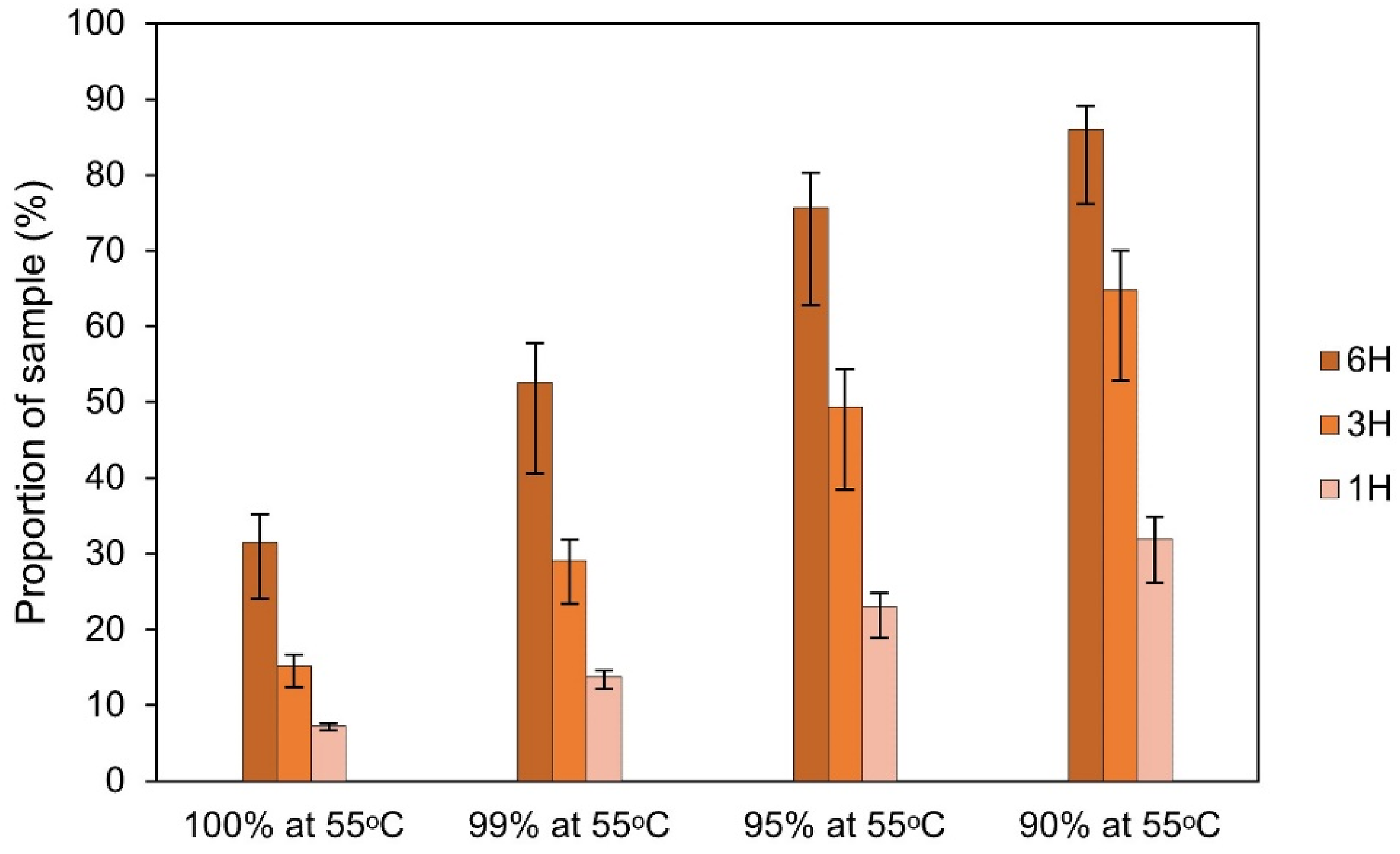
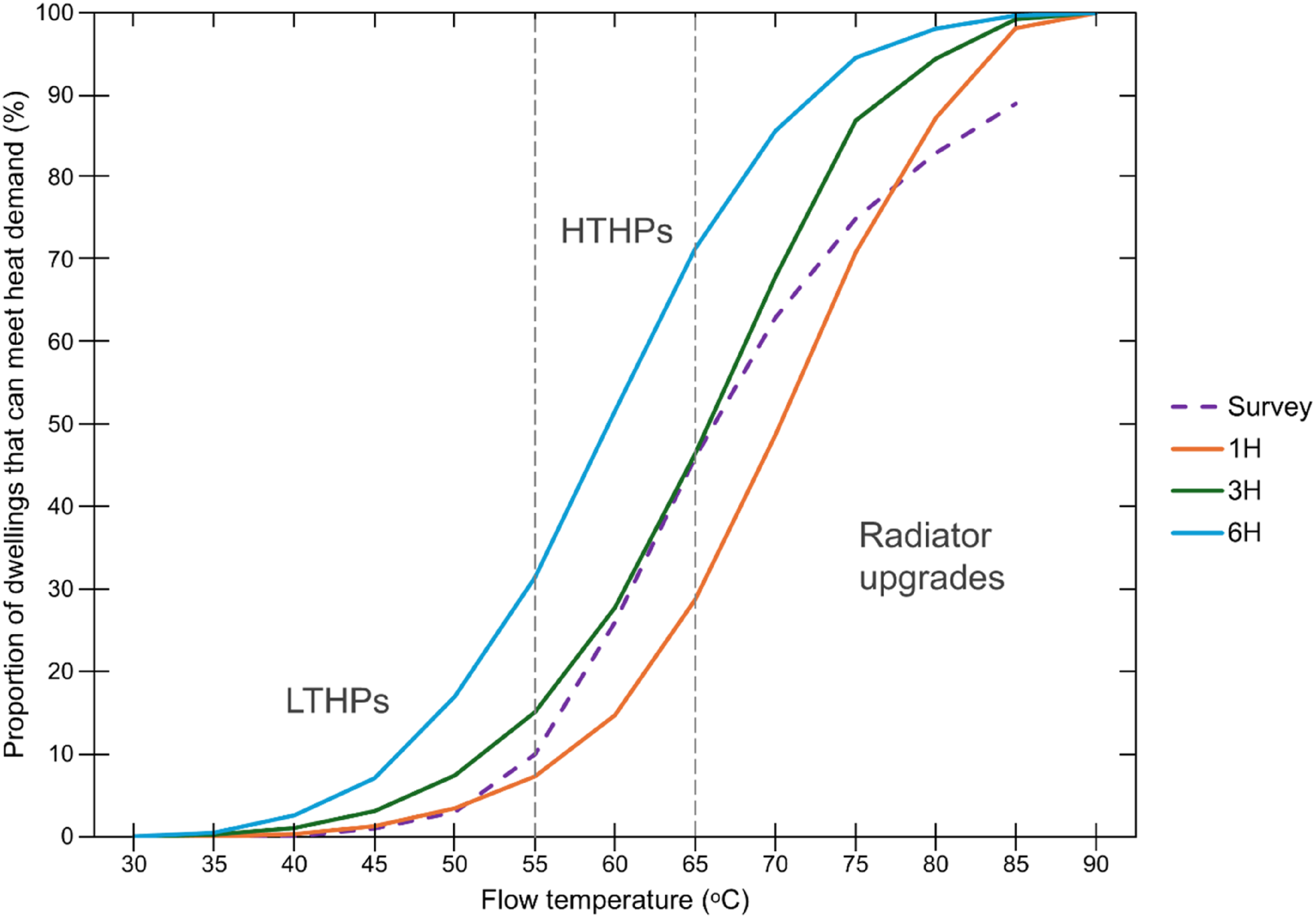
Finally, in Figure 9, the three averaging models are compared to the previous survey analysis by BEIS,
2
in their predicted proportion of UK dwellings that could meet peak heat demand at various flow temperatures. Comparing the models shows that when averaging the heat demand over 6 hours, dwellings can clearly meet heat demand at lower flow temperatures than previously predicted by survey analysis. However, averaging heat demand over 3 hours suggests a more marginal increase in heat pump ready dwellings, with intersection with the survey analysis curve at around 65°C. Furthermore, when only averaging heat demand over 1 hour, the model suggests that less dwellings are ready for a heat pump without radiator upgrades than predicted previously in survey analysis. This reiterates the usefulness of running heat pumps over longer time periods, which may require changes in when heating is scheduled, compared to previous boiler operation. A set of cumulative distributions showing the predicted proportion of UK dwellings which could meet heat demand at various flow temperatures for the three different averaging models, and the original survey model applied in BEIS
2
.
Discussion
The results from this analysis contribute to understanding the ability of existing heating systems in the UK to operate at lower flow temperatures without emitter or fabric upgrades, specifically by using real heating system performance data rather than surveys. The analysis is also for a greater sample size than previous research by BEIS, 2 with approximately 4600 boilers analysed compared to 515 dwellings surveyed. It was assumed that the dataset approximates UK gas heating dwellings as a whole, based on the distribution of boilers annual space heating demand not being vastly different to national scale modelling (Figure 1). Finally, the difference in results between BEIS, 2 which used surveys to predict the required flow temperatures in UK heating systems, and this research which used boiler performance data, demonstrates the potential impact of performance gaps. Whereby, surveys could potentially overestimate the necessity of radiator upgrades with heat pumps, which adds to the costs and disruption for heat pump roll out.
Limitations
When examining model outputs and their implications, it is important to consider the robustness and limitations of the model.
Heating system thermal mass estimation
Thermal mass was estimated empirically by the amount of gas power input required to raise the flow temperature in warm up from cold periods and was used in estimating the power output of heating systems and subsequent underlying heat demand. Estimated thermal mass was situated within physically sensible values for heating systems, with litres of water equivalent between 20 and 350L, with most being between 50 and 120L. Thermal mass estimates also correlated with peak heat demand (Figure 11, appendix) – providing some validity to the method, as larger properties will likely have larger heating systems and higher heat losses. Furthermore, although estimated thermal mass was expected to be an overestimate (Estimating heating system thermal mass and underlying heat demand), a 20% lower thermal mass was modelled but was found to have a negligible impact on the results.
Assumptions of internal temperatures and flow-return temperature difference
Estimation of required flow temperature required assumptions on internal temperature and the heating system temperature drop to be made. In a baseline case, an internal temperature of 20°C and a heating system temperature drop of 8°C was used. Internal temperatures are commonly cited as varying between 18 and 22°C, so 20°C is reasonable. Furthermore, the heating system temperature drop was selected based on the average temperature drop during heating system operation. Moreover, the uncertainty imposed from not knowing these temperatures was modelled as a sensitivity, between 18 and 22°C internal temperature and 2-22°C heating system temperature drop, with the latter based on the range seen in boilers with return temperature data (Figure 11, appendix). The impact of the uncertainty in internal temperature and heating system temperature drop can be seen in Figures 7 and 8 as error bars. This modelled uncertainty does not change basic interpretations of the results and has a larger impact when estimating lower required flow temperatures (e.g. less than 55°C). It is also worth noting that the flow rate and heating system temperature drop in a heat pump heating system is likely to be different to that of incumbent boiler heating systems, typically with higher flow rates and lower temperature drops with heat pumps compared to boilers. The change in heating system temperature drop was not modelled in estimating uncertainty, however the drop of 8°C used coincidentally is the same as that used in MCS heat pump design processes 14 and may therefore approximate the required design flow temperature.
Radiator cooling rate
Modelling heating system output, and underlying heat demand, required estimation of radiator cooling rates. This was done simplistically, by interpolation between flow temperature values when the heating system pump was off. This may result in lower cooling rates at the start of radiator cooling, compared to more physically realistic exponential cooling. Hence, this may impact estimates of underlying heat demand, and is seen as a limitation requiring further work on the uncertainty in cooling rates. However, its impact may be limited for higher averaging periods.
Domestic hot water events
A simple filter to remove domestic hot water events was used in this analysis. This was necessary to remove interaction between hot water events and space heating, where it is difficult to unentangle the contribution of space heating output, however, this approach assumes there is negligible space heating demand during hot water events.
Representativeness of monitored data
The model uses in situ radiator performance in averaging intervals, to predict required heat pump flow temperatures for continuous heating. The operational conditions during this time may not necessarily be representative of average or normative conditions, for example, some radiators could be shut off . However, this is more representative of real heating system performance and operation, and filtering for heat outputs above 1 kW enabled transient warm up periods to be avoided. Further, prediction of required heat pump capacities and flow temperatures was for like for like heat demand, where there is possibility that occupants under or overheat their homes. It may also be possible that occupants were underheating their homes more than in previous years, considering the data used was after the energy crisis, for the 2021-2022 heating season. Despite this, it is argued that this is an advantage, to incorporate the real use of heating systems in the modelling, as this can highlight the differences in expectations of design and real use of heating systems.
Nonetheless, this is the largest study of its kind, with a sample of approximately 4600 boilers, in comparison to 515 radiator capacity surveys in BEIS. 2 There will be some sampling bias in each of theses studies, so some differences between the two could arise from this. Specifically, the boiler heated dwellings were all located in England, whereas the surveys from BEIS 2 also included dwelling archetypes from Wales, Scotland, and Northern Ireland. This means the comparison between the two analyses is not for the same population of buildings. However, considering the distribution of annual boiler space heating demand in Figure 1, the large sample size, and the fact that England is the most populous country within the United Kingdom, it is believed that this study provides the best current picture of the heat pump readiness of existing heating systems in the UK.
It is also worth noting that UK winters are expected to become milder on average, due to changing climate, hence the single year of boiler data only offers a brief cross section for prediction of current heat distribution system requirements. This gradual effect will likely ease flow temperature requirements of existing heating systems further over the majority of the heating season, however there is uncertainty over how much winter extremes will be affected, with heating system sizing based on meeting peak heat demand.
Additional barriers to heat pump installation
Considering this together, this analysis gives insight that for the real performance and operation of heating systems in the UK, it appears that more existing heating systems can have a heat pump installed without emitter upgrades than that modelled using surveys. 2 This should mean that more heat pumps can be installed for a cost within the UK’s £7500 BUS grant than previously thought. However, it is difficult to estimate the true impact for a number of reasons. Firstly, the analysis used data on the whole heating system, and it is possible that radiator sizing varies across the dwelling. Hence, it is impossible to know if a few critically undersized radiators need replacing17,18 or if the entire heat distribution system needs replacing, with very different costs required. Secondly, additional equipment beyond radiator and fabric upgrades may be necessary when installing a heat pump and can also significantly increase costs and disruption. 3 For example, buffer vessels and/or new pipework can be required to account for changing hydraulic conditions with a heat pump, and a domestic hot water cylinder (or a replacement cylinder) could be necessary to meet DHW demand at lower flow temperatures. Legionella prevention is not considered an issue as low temperature heat pumps can perform weekly pasteurisation of hot water cylinders using an immersion heater. Thirdly, beyond equipment costs, there may be additional factors contributing to heat pump readiness, for example – the available space for a heat pump, noise considerations, electricity grid constraints, and occupants willingness to adopt different heating patterns and use of the heating system.
Furthermore, beyond understanding the upfront costs of heat pump installation, it is also important to consider heat pump efficiency. In this study, the trade-offs between higher heat pump efficiencies at lower flow temperatures, and necessity of radiator upgrades was not investigated, but could be in future work, using analogous methods to Watson & Bennett. 9 Appreciating this will be important to understand the impact on running costs, peak electricity demand, and – understanding when a HTHP is more economical than a LTHP. In effect, it is possible that a HTHP could be installed with no radiator upgrades in a dwelling, but it may be economically beneficial to replace some relatively undersized radiators and lower the flow temperature further, based on improvements in efficiency and return on capital investment via lower operating costs.5.1.7. Practical interpretation
After bearing these limitations in mind, it is thought that the true number of dwellings ready for rapid retrofit of heat pump heating systems lies in between the six hourly averaging model presented here and the previous analysis by BEIS, 2 easily compared for their prediction of radiator upgrade requirements in Figure 9. The 6 hour averaging model is considered the more reasonable model for predicting radiator requirements using the boiler dataset, because it appropriately represents the longer heating periods expected with heat pumps. It is thought a more accurate prediction of heat pump readiness will lie between these two analyses because this analysis only uses a single year of data, and may not capture peak heat loss, and occupants may underheat their dwellings relative to recommended levels. Despite this, this analysis is the largest of its kind, and overcomes the limitations of previous survey analysis by using measured performance data, rather than effectively assuming the thermophysical performance of radiators and building fabric which is necessary when surveying a dwelling. Hence in summary, this analysis suggests the costs of heat pump installations could be lower with less radiator and fabric upgrades, if only aiming to provide like for like heat load, and if having sufficient data to more accurately design the future heating system.
Moreover, the differences between estimations of minimum required flow temperature and heat load by this empirical analysis and previous survey analysis demonstrates the implications of uncertainty in modelling heat loss and heating system performance. Further research and development of hybrid models, using a mix of survey and data-driven techniques could help produce a more precise design process. Doing so could lead to more accurate specification of heating systems and enable more cost-effective design of low carbon heating, essential for an effective and efficient nationwide roll out of heat pumps. Currently, this research will not change anything in practice, because real installations use surveys to design heat pump systems, which appear to oversize radiators relative to what may be required for occupant set heat demand. Furthermore, evaluating if cost minimisation via minimal radiator upgrades is desirable is important, as there are benefits to larger radiators, such as improved heating system efficiencies which will reduce running costs, carbon emissions, and strain on the electricity grid. Finally, any future change in processes will require vigorous validation and piloting of novel methods, to ensure they improve design and can be implemented with ease.
Conclusion
A novel model was developed to estimate the flow temperature and heat capacity requirements for approximately 4600 heating systems in the UK using existing diagnostic boiler data. The data was shown to broadly approximate national scale heat demand modelling in the UK, and was thusly assumed to indicate the necessity of radiator and fabric upgrades for nationwide roll out of heat pumps. Generally, the results indicate that there will be different requirements of fabric and emitter upgrades for different dwellings when installing heat pumps, which was already well known, but the extent of upgrades required appears lower than previous estimates using surveys. 2 For example, when averaging estimated heat demand over 6 hours (a significantly more ‘continuous’ heating profile), the model estimated that 31.5% of dwellings could operate at 55°C or less, without radiator upgrades, compared to 10% estimated by surveys in BEIS. 2 In this same model, the number of dwellings ready to operate at 65°C or less without radiator or fabric upgrades climbs to 66.5%, compared to 46% estimated by surveys in BEIS. 2 Hence, up to two thirds of dwellings in the UK could be ready for High Temperature Heat Pumps (HTHPs), with approximately one third of these same dwellings ready for Low Temperature Heat Pumps (LTHPs), provided that heating system controls can enable successful spreading of the heat load over 6 hours. The models heat demand averaging interval was also found to be important (representing changes to heating schedules), with higher averaging intervals (longer heating periods) resulting in greater flow temperature reduction potential, demonstrating the importance of changing heat patterns when converting to a heat pump from a gas boiler. Furthermore, only a very small amount of the heating season required the highest flow temperature, highlighting the potential of small-scale hybridisation to reduce the requirements for heat pump installations, where only a very small portion of the year effectively dictates the necessity of radiator or fabric upgrades. Altogether, these results suggest that the costs and disruption for nationwide deployment of heat pumps can be lower than previously thought, but that this would not be possible to know without use of real performance data. Hence, this raises questions about the efficacy of existing design practices, while simultaneously demonstrating potential for a future data-driven testing procedure to more precisely design and retrofit future heat pump heating systems.
Footnotes
Acknowledgements
This research was made possible by support from the EPSRC Centre for Doctoral Training in Energy Resilience and the Built Environment, grant number EP/S021671/1, with additional doctoral funding provided by Passiv UK Ltd. Analysis by the primary author was conducted while on secondment at the Department for Energy Security and Net Zero. The authors would like to kindly thank Bosch Thermotechnology Ltd for providing access to the diagnostic boiler data used in this research.
Declaration of conflicting interests
The author(s) declared no potential conflicts of interest with respect to the research, authorship, and/or publication of this article.
Funding
The author(s) disclosed receipt of the following financial support for the research, authorship, and/or publication of this article: This work was supported by the EPSRC (EP/S021671/1).
Correction (February 2025):
In this article, special collection heading has been corrected from “CIBSE Technical Symposium 2024” to ‘Delivering buildings and defining performance for a net zero built environment’.
Appendix
A plot between estimated thermal mass (in litres of water equivalent) and maximum heat demand (kW) for 6-h averaging. The line shows the results of a least squares regression analysis, with the R2 value displayed.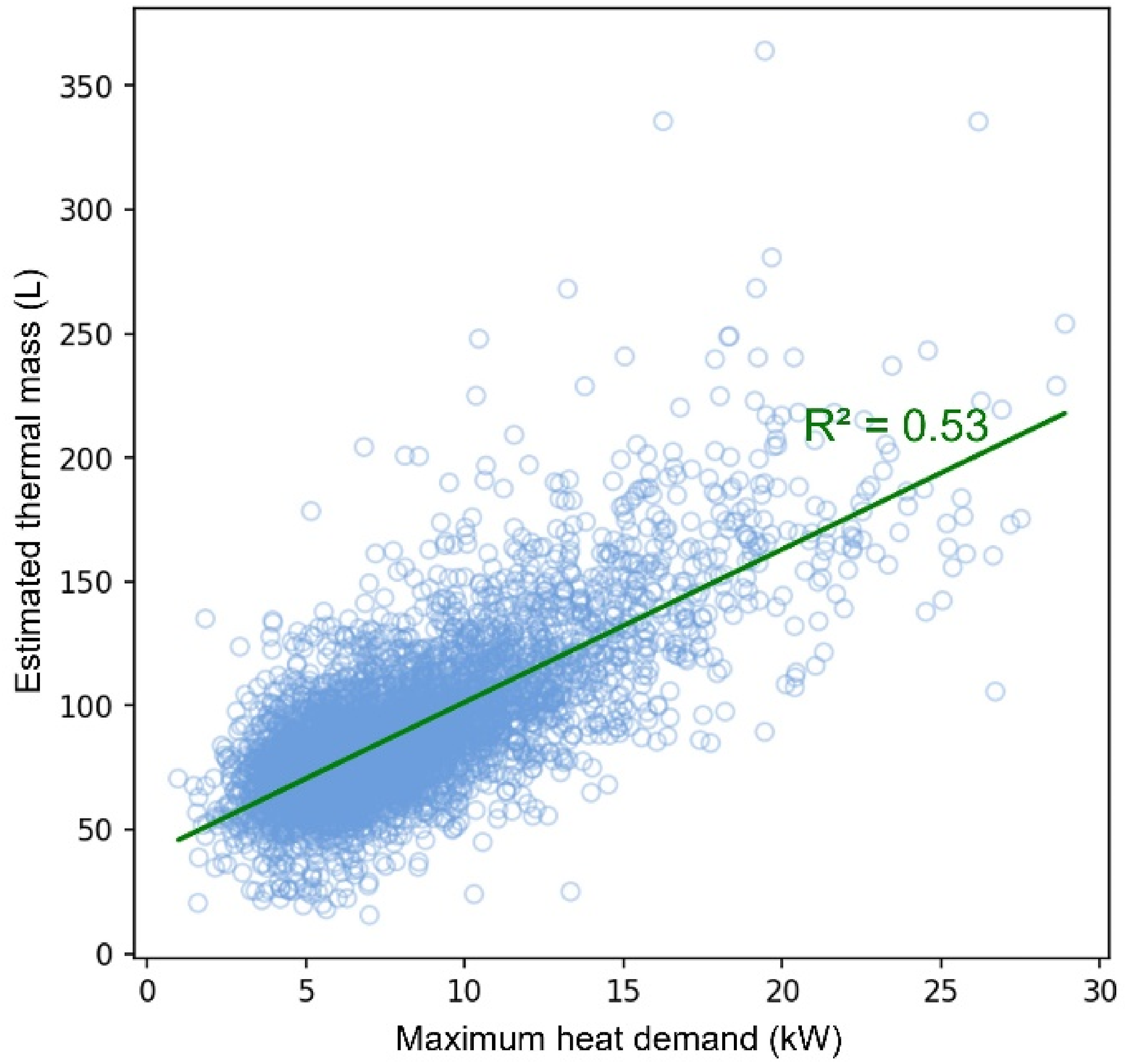
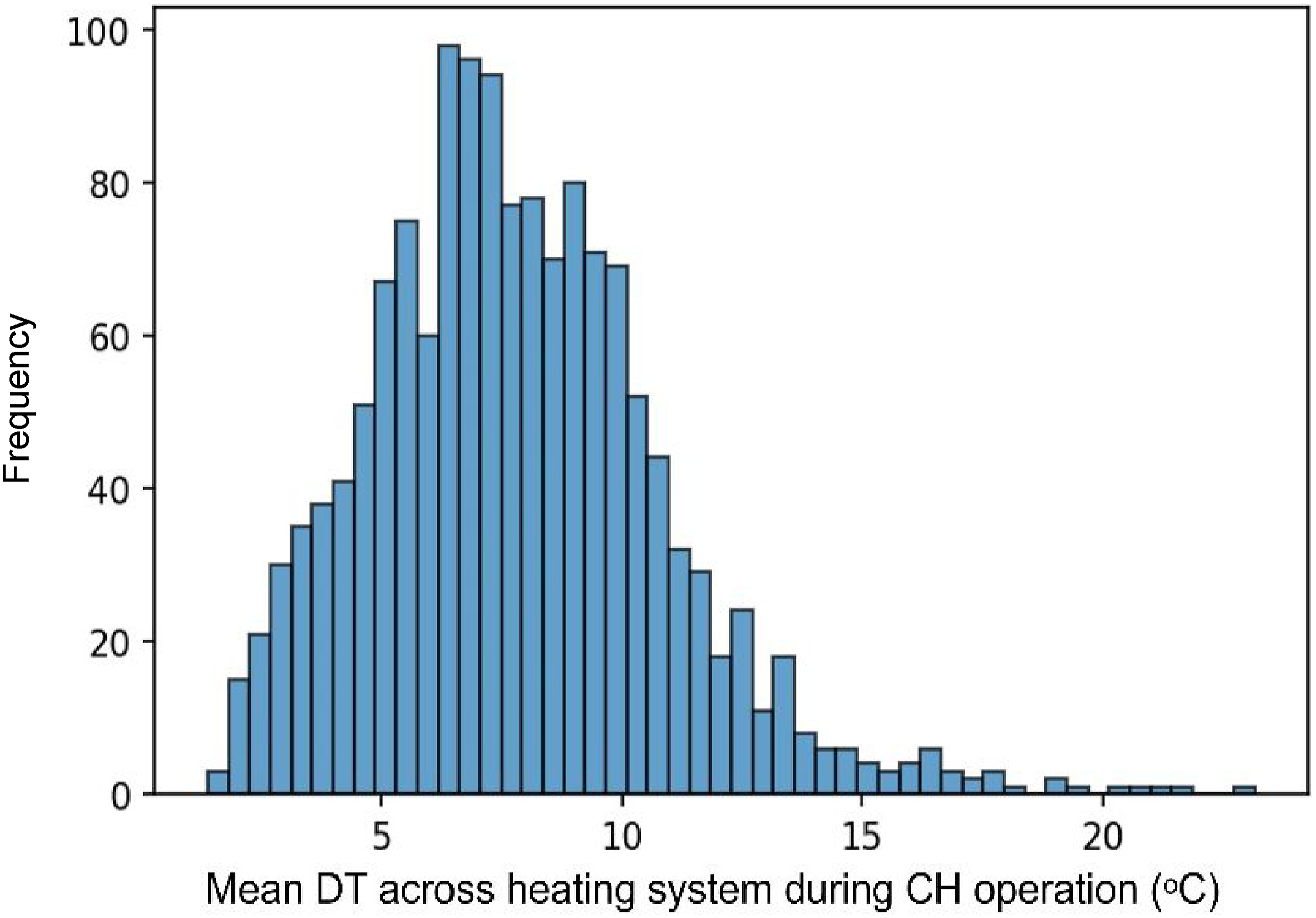
A histogram displaying the distribution in mean heating system temperature drop values when the boiler was in central heating mode. This is for the 29% of boilers with return temperature data.