An energy analysis methodology for residential heat pump retrofits

Abstract

The government has targets to upscale domestic heat pump retrofit as part of the strategy to decarbonise heat. There are significant barriers to uptake including installation cost together with a lack of expertise in predicting and reporting energy and carbon performance. As a result, end user confidence in heat pumps can be low. This paper presents analysis of two monitored domestic properties using high resolution data. The aim is to develop reliable prediction and in-use diagnostic tools to improve transparency and reliability of heat pump performance. This paper focuses on a method drawn from theory as set out in CIBSE TM41, and shows how real building heat loss coefficients can be determined from regression analysis over different time frame resolutions.

Practical application

This research aims to provide residential heat pump retrofit providers with cost effective methods for assessing the suitability of dwellings to accept heat pump retrofit solutions, and to extend these techniques for the effective monitoring and performance evaluation of heat pumps post installation.

Introduction

LSBU (London South Bank University) is working with Parity Projects as part of a consortium on a DESNZ (Department for Energy Security and Net Zero) funded Heat Pump Ready Stream 2 project. ¹ The consortium comprises, in addition to LSBU, companies that advise and deliver domestic energy retrofit solutions, a heat pump manufacturer and an energy consultancy. The project aim is to raise levels of confidence for heat pump retrofit solutions in domestic dwellings through better analytics. The project outcomes will include tools for improved economic heat pump sizing, together with monitoring methods that produce specific performance metrics. It will be necessary to be able to demonstrate whether different-from-expected performance is due to system deficiencies, weather effects (particularly temperature and wind speed and direction), or user behaviour. Two research teams, one at the retrofit solution provider and one at LSBU, have explored different approaches to modelling the heating energy performance of dwellings in order to both predict how a heat pump will perform (in terms of cost, carbon and comfort), and also show how these models can be used to track and verify that predicted performance is being delivered post-retrofit. The project has installed extensive remote monitoring systems into 20 houses (mainly older detached properties).

Both approaches have a number of things in common in that they both:

• Use high quality monitored data to analyse energy flows in dwellings.

• Use this data to validate the modelling methodology being employed.

• Attempt to identify and quantify the building thermal characteristics, in particular the heat loss coefficient (HLC) and the effective thermal capacity of the structure from measured values of energy, temperature and heat gains.

• Characterise the impact of casual heat gains into the space.

• Determine the efficiency of the heat generator (boiler or heat pump).

• Identify the levels of uncertainty in the results in order to make measurable impact statements about heating system performance.

This paper presents the LSBU analytical methodology, which is based on CIBSE Technical Memorandum (TM) 41. ² The focus is on examining how well a degree-day based approach can reveal accurate assessments of building heat loss coefficients and heating system efficiencies, while accounting for factors such as building thermal capacity and casual heat gains. TM41 differs from traditional degree-day approaches by applying a first order lumped parameter method to calculate the mean time-varying internal temperature as the driver for heat loss, rather than the internal set point temperature. The data from this study has allowed a detailed analysis of how this model can replicate actual temperature variation within the building. Morris et al ³ conducted such a study, in parallel with the work of this paper, in order to validate the TM41 methods for the prediction of future energy use. This also examined how to quantify the effective thermal capacitance of the houses, which is a value not easily identified by other modelling methods.

The work in this paper uses historical internal temperatures in order to conduct the HLC assessments. Note that by using actual internal temperatures it is not necessary to explicitly know the thermal capacitance, as its impact is manifest in the way temperatures vary over time. This paper therefore represents a method for baselining a house’s energy performance prior to predicting future energy use. Results are shown for two properties to demonstrate how analysis time frames (daily, weekly or monthly time periods) impact the results, and the implications this can have on the practicalities of predicting and monitoring retrofit heat pump performance.

Theory and method

Theory

There has been a significant increase in efforts to use metered energy of actual dwelling to establish the actual heat loss coefficient (HLC) for a building, for example in the SMETER and related trials.^4–6 Most of these use regression analysis of heating energy consumption (e.g. through smart gas meter data) against outdoor temperature. These methods have to make adjustments for heat gains (e.g. solar gains) and thermal storage effects to account for scatter in the data and to obtain reliable estimates of the HLC.

TM41 employs similar principles, using a lumped parameter approach to thermal mass, and making reasonable assumptions about casual heat gains. The difference with SMETER approaches is that TM41 incorporates these factors into the regression independent variable in the form of the degree-day. The crucial factor is the selection of the building base temperature from which degree-days are calculated.

The basic form of the model is expressed by equation (1) ²

$E=\frac{H}{\eta }=\frac{24\left(\mathrm{\Sigma }UA+\frac{1}{3}NV\right)\sum \left({\theta }_i-\frac{Q_G}{\left(\mathrm{\Sigma }UA+\frac{1}{3}NV\right)}-{\theta }_o\right)∆t}{\eta }$

(1)

where

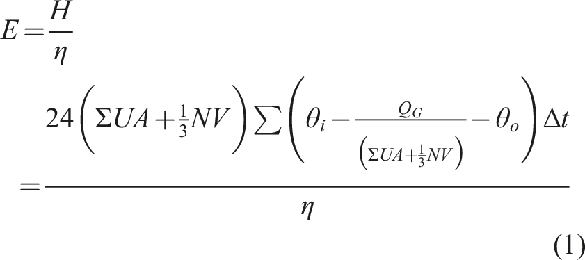
A is the area of a building fabric component – m²

E is the energy consumed over a defined period of time (day, week, month or year) – kWh

H is the heat delivered by the heating system to the space – kWh

N is the number of air changes per hour in the heated space due to infiltration or ventilation – h⁻¹

Q_G is the average casual (including solar) heat gain into the space – kW

t is the time interval under investigation – hours or days

U is the thermal transmittance of a building fabric element – W m⁻²K⁻¹

V is the volume of the space – m³

η is the overall heating system efficiency or COP

θ_i is the internal temperature of the building - °C

θ_o is the outdoor temperature - °C

The fabric and ventilation components can be combined into a single parameter, U′, (U′ = ΣUA+¹/₃NV), to give the overall heat loss coefficient (also called the HLC). The expression for gains divided by U′ can be interpreted as the temperature rise due to these gains, which in turn gives rise to the concept of a base temperature, θ_b, as follows

${\theta }_b={\theta }_i-\frac{Q_G}{U^{\prime }}$

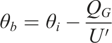
The base temperature is the outdoor temperature at which the heating system need not run to deliver the required indoor temperature. This enables the temperature-time component in equation (1) to be simplified to

$D_d=\mathrm{\Sigma }\left({\theta }_b-{\theta }_o\right)∆t$

where D_d is a quantity known as degree-days. This is true if Δt is one day, and θ_o is the external temperature that represent conditions on that day (e.g. the average outdoor temperature, although this is an oversimplification). In reality modern degree-days are calculated from the hourly outdoor temperature record to give degree-hours, D_h, which are divided by 24 to give degree-days. Degree-days are published from various sources for local weather conditions, and to various base temperatures (normally in 0.5 K steps).

This gives rise to the deceptively simple expression for equation (1) as follows:

$E=\frac{H}{\eta }=\frac{24U^{\prime }{D}_d}{\eta }$

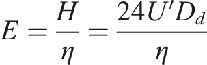
Plots of E against D_d have been used by the energy management community for decades in order to measure weather related energy performance of buildings. In theory the slope of a regression line of E v D_d is equal to the term 24U′/η. This principle can be applied to regression analysis to determine U′ (the HLC), N or η, depending on what information is known with any certainty. For example, U values are reasonably easy to determine from construction details, and η can be measured using heat and energy meters. (Note: the air change rate, N is the highly uncertain component of U′, and may vary greatly depending on how well a property is sealed, whether or not windows are opened, and on wind speed and direction. This can cause significant uncertainties in data regressions).

However, the above is only valid if the correct base temperature is used to generate D_d. The base temperature incorporates two critically important values: θ_i, which drives the rate of heat loss from the building, and Q_G, which offsets the amount of heat required from the heating system. Traditionally, the base temperature was calculated using the set point temperature for θ_i , but this does not adequately account for the usual case of intermittent operation of the heating system. Typically the system is switched off overnight to save energy consumption. The building is allowed to cool, thus reducing the average rate of heat loss over a 24 h period. The rate of cooling and subsequent re-heating depends on both the HLC of the building and its thermal capacity. Buildings with different thermal properties have different patterns of heating and temperature recovery rates. TM41 provides a method for calculating the mean internal temperature of a building using a lumped thermal capacitance method. There is some evidence that effective thermal capacitance actually varies throughout the year, with the implication that the HLC may also vary. ³ The results in this paper should be considered in the light of this possibility. Such variations in HLC and thermal capacity may explain some of the scatter exhibited in regressions (which can also be due to variations in heat gains and system control characteristics).

For a monitored house it is possible to directly capture these thermal capacity effects through the measured daily mean internal temperature. The mean daily gain temperature rise can then be subtracted from this to give the building specific base temperature. In standard degree-day practice the base temperature is assumed to be constant, whereas in reality gains vary from day to day and season to season. A key issue for this research is to determine the frequency of gain variation (mean daily, weekly or monthly values) that returns regression statistics for reliable estimates of the HLC (U′) and the system efficiency, η. This will dictate the level (and cost) of required monitoring equipment and data collection frequency, and the complexity of the required analytics. Ideally, this should be as simple and transparent as possible.

Regression analysis and metrics

Regression analysis examines the correlation of two variables: an independent variable (x) and a dependent variable (y). If the two variables are strongly correlated it can be said that changes in x will cause changes in y. The theory of heat loss from a building set out above expects just such a linear change in E as a function of D_d, provided that D_d captures the other key influences on E such as casual gains and variance in U′. Multiple linear regression can be conducted to look at variance in a dependent variable for a number of independent variables, but this gives multi-dimensional results which are difficult to apply, and are much less transparent. Clarity, transparency and ease of understanding are critical factors in proving energy performance to a non-technical person.

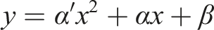
The standard linear regression gives an equation of the form

$y=\alpha x+\beta$

In our notation this maps as follows: y = E, x = D_d, α = 24U′/η, β = base load. Note that when E is space heating consumption only, β = 0.

The regression analysis also returns the coefficient of determination, R². This is a number between 0 and 1 where 1 indicates a perfect correlation (all points fall on the line of the equation), and 0 indicates no relationship. In practice values of 0.7 and above can be considered indicators of good correlation.

Note that simple linear regression assumes that the errors associated with scatter around the line are all assumed to be in the y values, and that no errors or uncertainties exist in the x values. There is an argument that the base temperature uncertainty provides exactly this difficulty, in which case Deming regression (in specific cases also known as orthogonal regression) should be conducted. ⁴ However, in our case the base temperature uncertainty is structural rather than random, and can be investigated, in theory, to remove these errors. Simple linear regression is used here for this reason.

For each regression conducted we want to assess how well the slope coincides with the calculated U′ by examining whether U′ = ηα/24.

Note that the calculated U′ value is used in determining the base temperature, which indicates an iterative approach can be used to get the calculated value and the slope to become equivalent (dependent upon the correct value of η).

Another important observation is the intercept. If solely space heating energy consumption is used then the intercept should equal zero. Where energy data include other loads (e.g. DHW (Domestic Hot Water)) the intercept should equal this average non-weather-related load. Departures from these theoretical values need to be investigated.

One other technique is available. The above discussion is based on a linear regression. If a 2nd order polynomial regression is used of the form

$y={\alpha }^{\prime }{x}^2+\alpha x+\beta$

it can be shown that the α′ typically turns from negative to positive with increasing base temperature. This implies there is a zero value of x² for some unique base temperature. It has been shown that this is a strong indicator of the correct base temperature. ² This occurs because at low base temperature (low degree-days) the points move towards the y-axis. As degree-days increase with increasing base temperature the points shift away from the y-axis, but the base load stays the same.

The above provides a number of tests for assessing the technique’s ability to characterise the building thermal performance parameters. The aim is to use these characterisations to settle on agreed actual (rather than calculated) values of U′, and to make informed assessments on the actual system efficiency, η. It is also aimed at finding the practical solar and other casual gain utilisation factors with greater certainty. Note that thermal capacitance effects are captured in the temperature data, and quantifying this capacitance requires much finer analysis resolution, ³ which is a secondary effect beyond the scope of this paper.

The above leads to the following metrics by which different sets of regressions can be assessed: α as a proxy for U′; β as a proxy for base (DHW) load, R² as an indicator gain capture, user behaviour and control performance, α′ as an indicator of linearity and overall model reliability.

Regression time frames

There are several options for time frame resolution. These are:

• Daily energy v daily degree-days.

• Weekly energy v weekly degree-days.

• Monthly energy v monthly degree-days (a preferred timeframe that aligns with billing frequency).

For each of these options there are further options on the resolution of base temperature

• Daily base temperature – calculating the base temperature each day, and using this to determine specific daily degree-days.

• Weekly mean base temperature – the average of the daily base temperatures for a weekly period.

• Monthly base temperature – the average of the daily base temperatures over a month.

• Whole heating season base temperature – the average of base temperatures from the entire data set.

• Arbitrary base temperature – typical current practice, but which can be modified by polynomial regression for α′ = 0.

Ideally we want to see high R² values, low or 0 α′ values and consistency for α and β across all timeframes. If, for example, monthly regressions can return reliable α and β values, it may not be necessary to go to the extra expense of daily energy analysis in order to verify the performance of a heat pump. If higher frequency is the better option, then specification of the minimum amount of monitoring kit required will be necessary.

Data collection and analytical process

The project has collected high volumes of data from a number of residential properties (the ultimate target is 40 properties). There are typically 14 or 15 data streams from sensors and meters in each property, each collecting data at 15 min intervals. In addition, each property has a weather station recording the following parameters at 5 min intervals: dry bulb temperature; humidity; wind speed and direction; global horizontal radiation; precipitation; barometric pressure. These high frequency data are of little practical use for this particular application (assessing monthly level energy bills). The data has been aggregated into either hourly averages (temperatures, solar irradiance) or hourly summations (energy, precipitation) for use in this regression analysis work.

The thermal response of a building to changes in outdoor temperature, usually referred to as the time constant, is measured in hours (sometimes days). Additionally the operating regimes of heating systems tend to repeat over 24 h periods, particularly in residential properties (commercial and institutional properties may have different weekend patterns). Experience has shown that plots of hourly energy use against hourly temperatures (degree-hours) produces high levels of scatter (poor R² values), and difficult-to-interpret regression statistics. ⁷ For these reasons the minimum time resolution for the analysis has been set at 24 h.

This requires the evaluation of daily mean internal temperatures, and daily mean casual gains to determine the daily mean base temperature. However, degree-days are calculated from the hourly outdoor temperature record, using the daily base temperature, as this most accurately captures those periods of the day when the heating system needs to operate.

The process used in this analysis is:

1. Calculate the building daily mean internal temperature from the area weighted room hourly temperature.

2. Determine the 24 h mean daily solar gains into the space from the measured solar irradiance (global horizontal in most cases). This needs to be adjusted to account for building orientation, solar aperture area and glazing transmission characteristics.

3. Determine other gains to the space, for example the 24 h average electricity consumption (that which occurs within the building), the occupants, and other forms of heat.

4. Calculate the gain temperature rise using these gains (2 and 3 above) and the calculated U′.

5. Calculate the daily base temperatures.

6. Use these values to calculate the mean weekly and monthly base temperatures, and the whole data period average base temperature.

7. Calculate daily degree-days for each of these base temperatures, using the hourly outdoor temperatures.

8. Aggregate each degree-day type to obtain weekly and monthly totals.

9. Aggregate the heating related energy data at each level – daily, weekly, monthly.

10. Plot scatter graphs of energy v degree-days for each base temperature and aggregation level.

11. Check regression statistics and look for outliers – investigate and explain as necessary.

12. Check the regression slope parameter, α, against the calculated U′. Where these differ change U′ to see the impact on the regression parameters.

13. The tests for the veracity of the degree-day model depend on the closeness of the slope to the U′, the closeness of the intercept, β, to zero (or the known base load), the R² value, and the plausibility of a fixed base temperature that can replicate the best results.

Results

For each property a survey was conducted to establish layout, age and construction details. These details were put into RdSAP ¹ to generate calculated HLC values. We present two case studies here to show how variation of the key inputs can influence the results and how regression analyses can be interpreted. The first case study is for a house with a gas boiler and fitted heat meter, while the second shows a house where an oil boiler was replaced by a heat pump.

Case study 1 – gas boiler

Table 1 shows the key attributes for house IL26 as obtained from the site survey and a RdSAP analysis. The house employs a 24 kW combi boiler and has a heat meter fitted to the space heating (SH) circuit. The results presented here are for the delivered space heating energy only, and not gas consumption. This is because the DHW heat meter was not working, and boiler efficiencies could not be assigned to the SH component only. The values of α in this analysis therefore do not include efficiency effects. Useful data for this property covers the period 6/12/22 to 14/06/24.

Table 1.

Survey information for house IL26.

Type of house	Semi-detached
Location	Surrey
Age	55-65 years
Floor area	113 m2
Number of bedrooms	3
Glazing type	Double (17 m2)
Survey heat loss coefficient, U′	339 W K−1
Thermal capacity	Not known kJ/K
Time constant	Not known h
Heating type	Gas combi boiler (24 kW) + underfloor electric heating in selected areas
Heat loss at design Δθ	8151 W
Ancillary heating	Wood burning stove (not used)

Figure 1 shows the initial plot of daily space heating delivered energy against daily degree-days calculated to individual daily base temperatures. The gains into the space include assumptions about occupant levels, measured average general electrical loads, and measured solar gains multiplied by an assumed solar gain factor (SGF) (More detail on determining specific SGFs can be found in Morris et al ³ ). In this particular case the general electrical loads include the underfloor heating, so this energy contribution is captured in the base temperature calculation rather than being added into central heating delivered energy. Either approach should yield the same HLC estimate. [Note: polynomial regression lines and equations are shown on the following figures to indicate the linearity of the data – the ideal case would show α′ = 0. The polynomial R² values are omitted for clarity.].

Figure 1.

Daily space heating energy against daily degree-days to daily base temperature for IL26, U′ = 339 W K⁻¹, SGF = 0.5.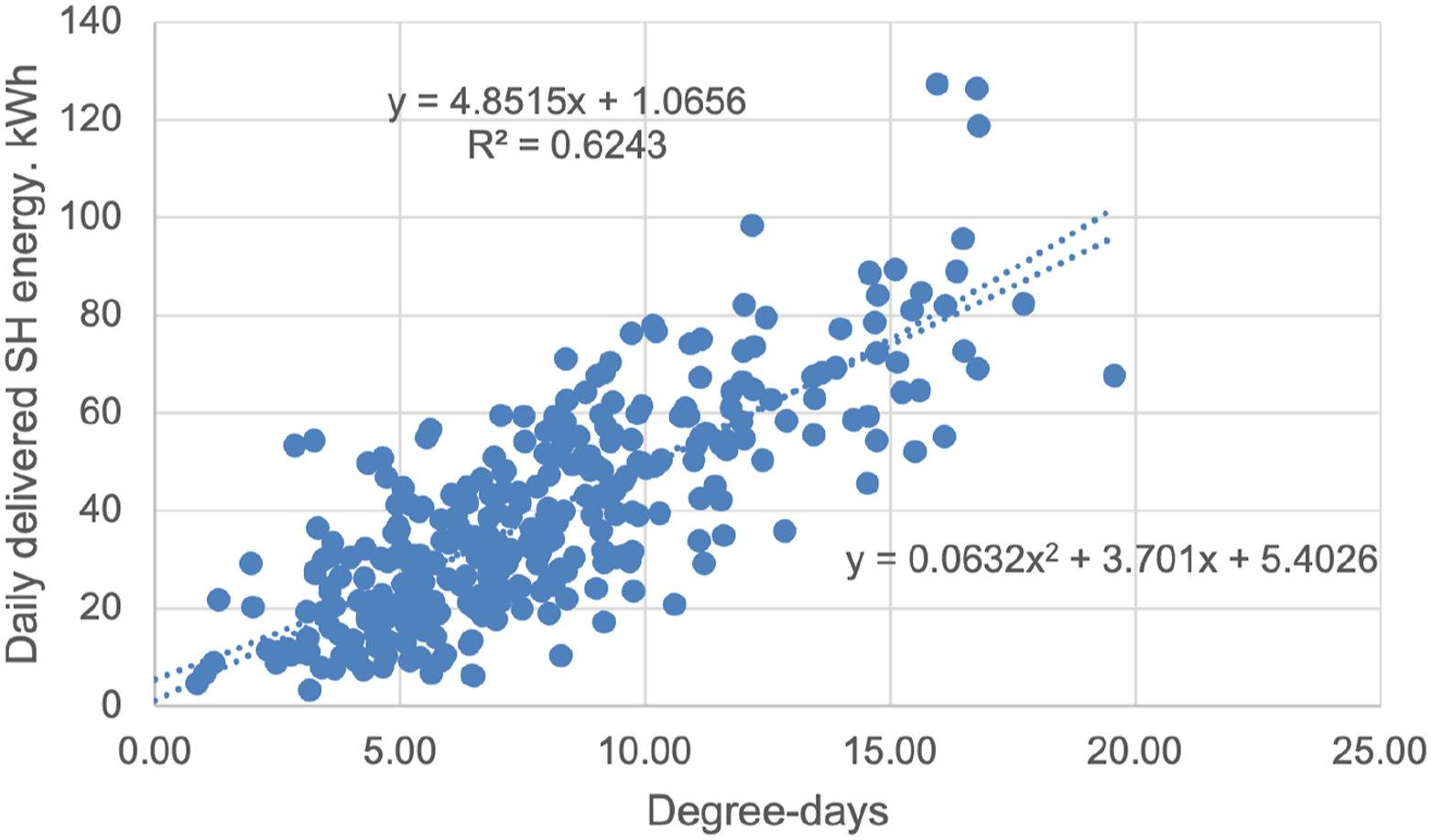

The data in Figure 1 shows a reasonable degree of linearity (low α′) although the amount of scatter is notable (R² ∼ 0.6). β is near zero, as would be expected. The important observation is that α appears low. According to the survey data we would expect to see a slope of 24 × 0.339 = 8.136 kWh/D_d, but we observe α = 4.8515 kWh/D_d. To reconcile this discrepancy an iteration of the base temperature calculation is required where the ratio Q_G/U′ (the gain temperature rise) is adjusted until the input U′ agrees with the value α/24. For this data set this occurs at a value of U′ = 186 W K⁻¹, some 45% lower than the RdSAP calculated value. Figure 2 shows the regression with the revised U′. Given the linearity of the results it is reasonable to infer that this is a better estimate of U′ than the RdSAP calculated value. The temperature record shows that the building is never underheated. One issue here is that β is now higher, and this infers a base load that does not exist, which requires further attention.

Figure 2.

Daily space heating energy against daily degree-days to daily base temperature for IL26, U′ = 186 W K⁻¹, SGF = 0.5.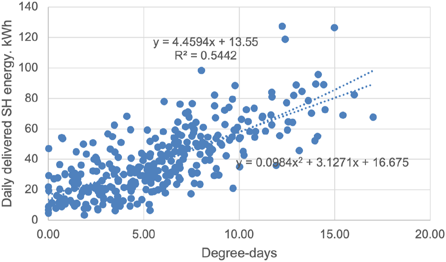

Figure 3 shows the results for weekly aggregated space heating energy and degree-days. The key observations here are that the slope has increased, indicating a higher HLC, and the R² is significantly higher (∼0.8). The reduced scatter is to be expected as individual days can be strongly influenced by occupant effects or environmental factors that can balance out over several days (these effects have been specifically observed in some of the data sets). This result suggests that weekly time resolution may be reliable for building and energy characterisation. However, this result does use specific daily gain information, and a further question for the study is whether weekly or monthly average gains can be used as reliably.

Figure 3.

Weekly space heating energy v weekly degree-days to daily base temperature for IL26, U′ = 186 W K⁻¹, SGF = 0.5.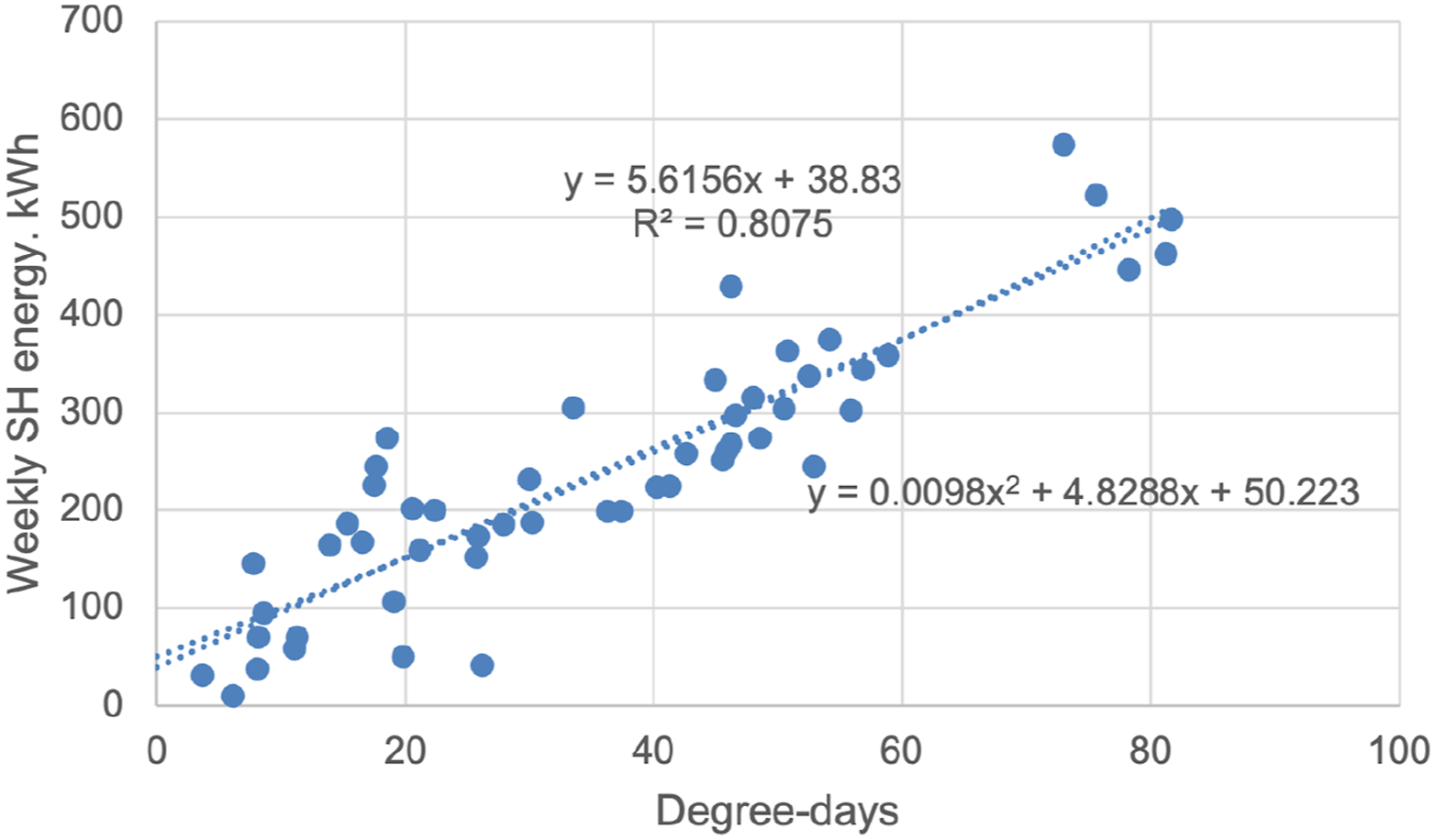

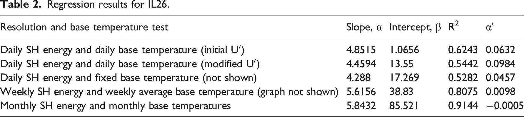
Figure 4 shows aggregated monthly regressions, with degree-days calculated to mean monthly base temperatures. The slope increases further (indicating an HLC of 243 W K⁻¹), while the R² and α′ values improve over the weekly values. Increasing slope with longer timeframe aggregation is a feature observed for all properties in this study, and in this case shows a variation of 30% between lowest and highest estimates. The explanation may lie in aggregation removing day-to-day variability to provide a better measure of mean HLC. Daily scatter may be due to weather effects (particularly wind), casual gain characteristics or behavioural issues (e.g. control adjustments). The selection of which HLC value to use for modelling future energy use will be the subject of further work in this project. A summary of results for this property can be seen in Table 2.

Figure 4.

Monthly space heating energy v monthly degree-days to monthly base temperature for IL26, U′ = 186 W K⁻¹, SGF = 0.5.

Table 2.

Regression results for IL26.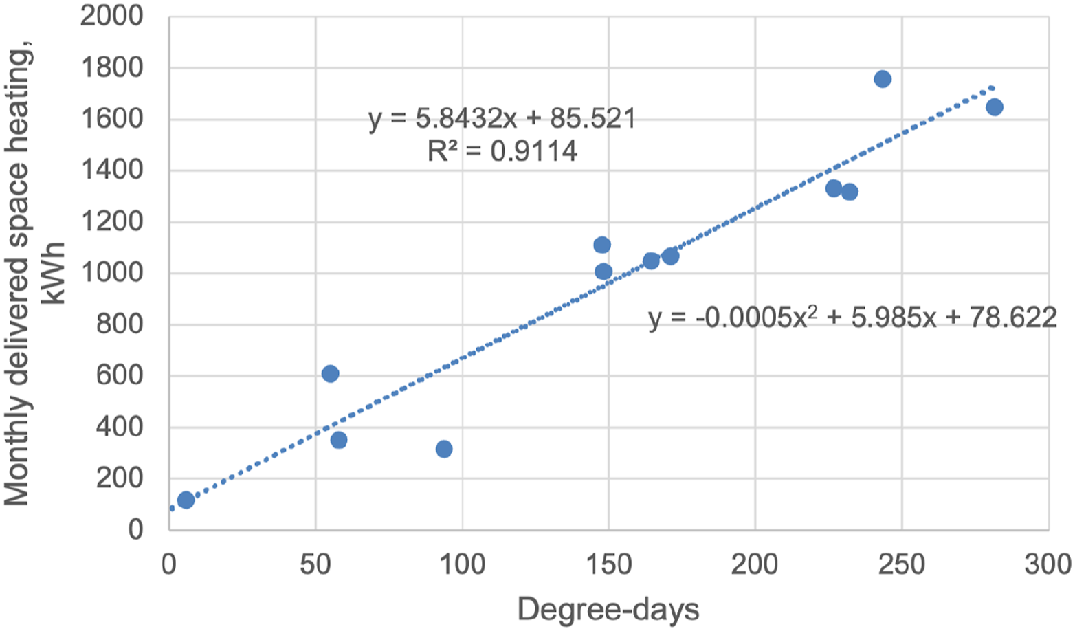

Resolution and base temperature test	Slope, α	Intercept, β	R2	α′
Daily SH energy and daily base temperature (initial U′)	4.8515	1.0656	0.6243	0.0632
Daily SH energy and daily base temperature (modified U′)	4.4594	13.55	0.5442	0.0984
Daily SH energy and fixed base temperature (not shown)	4.288	17.269	0.5282	0.0457
Weekly SH energy and weekly average base temperature (graph not shown)	5.6156	38.83	0.8075	0.0098
Monthly SH energy and monthly base temperatures	5.8432	85.521	0.9144	−0.0005

Case study 2 – heat pump retrofit replacing oil boiler

Table 3 shows the key attributes for house IC260 as obtained from the site survey and RdSAP analysis. This house comprises an 18th century core with some additions and upgrades. Cavity wall insulation and double glazing are fitted throughout. The property originally had oil fired central heating, which was replaced in March 2023 with an 11 kW air source heat pump. Limited data is available for the oil regime, but this serves as an example of a retrofit comparison. An in-line oil flow meter was fitted to the boiler just over one month before the heat pump installation. Prior to that oil usage was measured from a ten-step oil gauge and bulk oil deliveries.

Table 3.

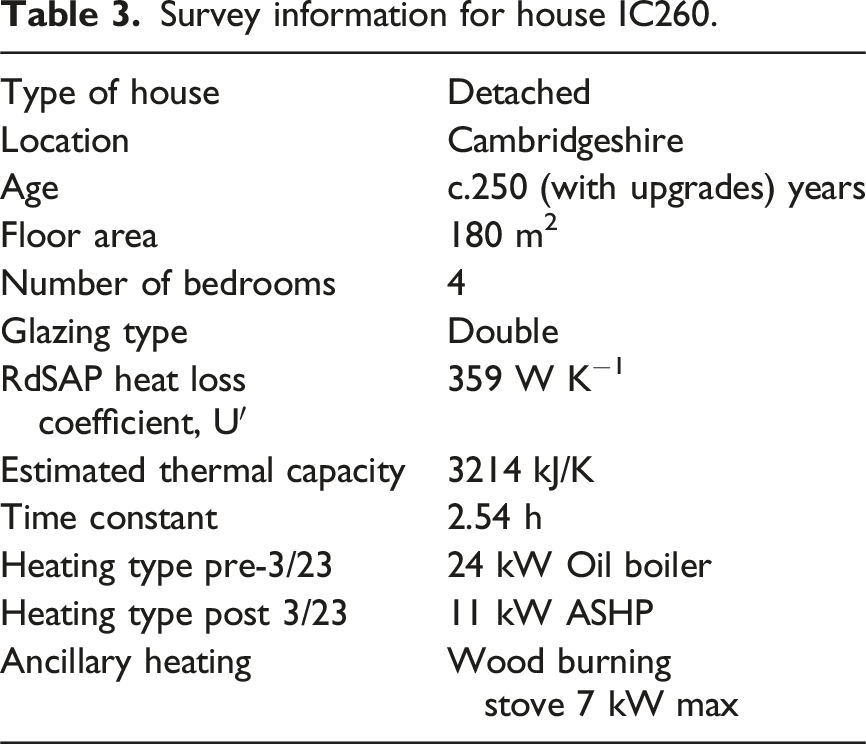
Survey information for house IC260.

Type of house	Detached
Location	Cambridgeshire
Age	c.250 (with upgrades) years
Floor area	180 m2
Number of bedrooms	4
Glazing type	Double
RdSAP heat loss coefficient, U′	359 W K−1
Estimated thermal capacity	3214 kJ/K
Time constant	2.54 h
Heating type pre-3/23	24 kW Oil boiler
Heating type post 3/23	11 kW ASHP
Ancillary heating	Wood burning stove 7 kW max

Oil boiler analysis

Figure 5 shows 39 days of oil meter data against daily degree-days to daily base temperatures. High scatter and poor linearity are apparent (low R² and high α′). The value of β is high at 29.1 kWh/day, but daily DHW energy from summer use has been shown to be around 2 L (∼21 kWh) (indicating a very poor boiler and system efficiency. The value of α = 7.6719 kWh/D_d, assuming a boiler efficiency of 0.85, would indicate a value of U′ of around 271.7 W K⁻¹, which is ∼25% lower than the RdSAP calculated value. An analysis using bulk oil delivery returns a value of U′ = 346 W K⁻¹, considerably closer to the calculated value. The bulk delivery analysis includes over 2 years of data, and may be a better indicator, but contains more assumptions. This indicates the difficulty of obtaining reliable baseline data for oil boiler installations.

Figure 5.

Daily oil use against daily degree-days to daily base temperature for house IC260, U′ = 346 W K⁻¹, SGF = 0.5.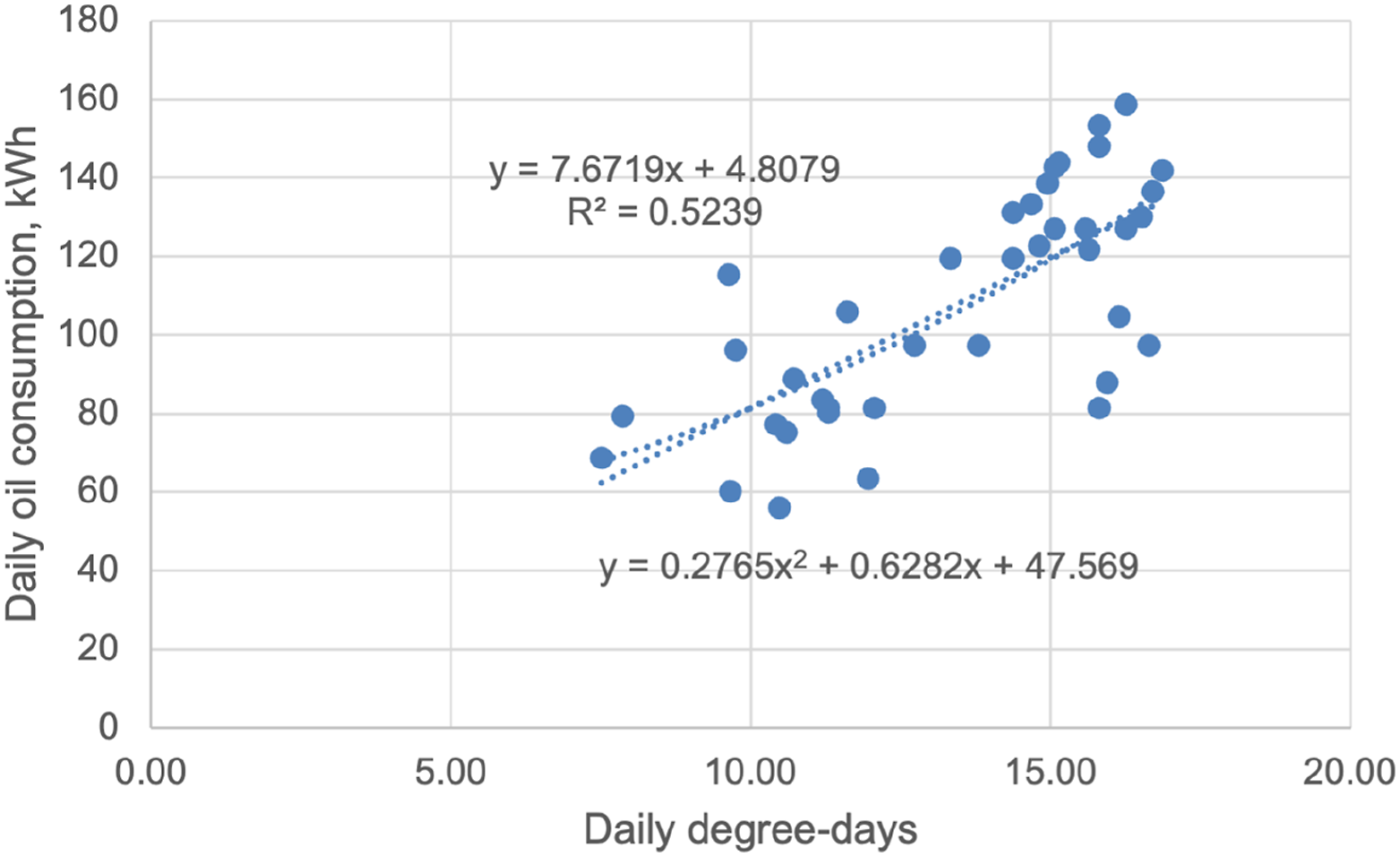

Heat pump analysis

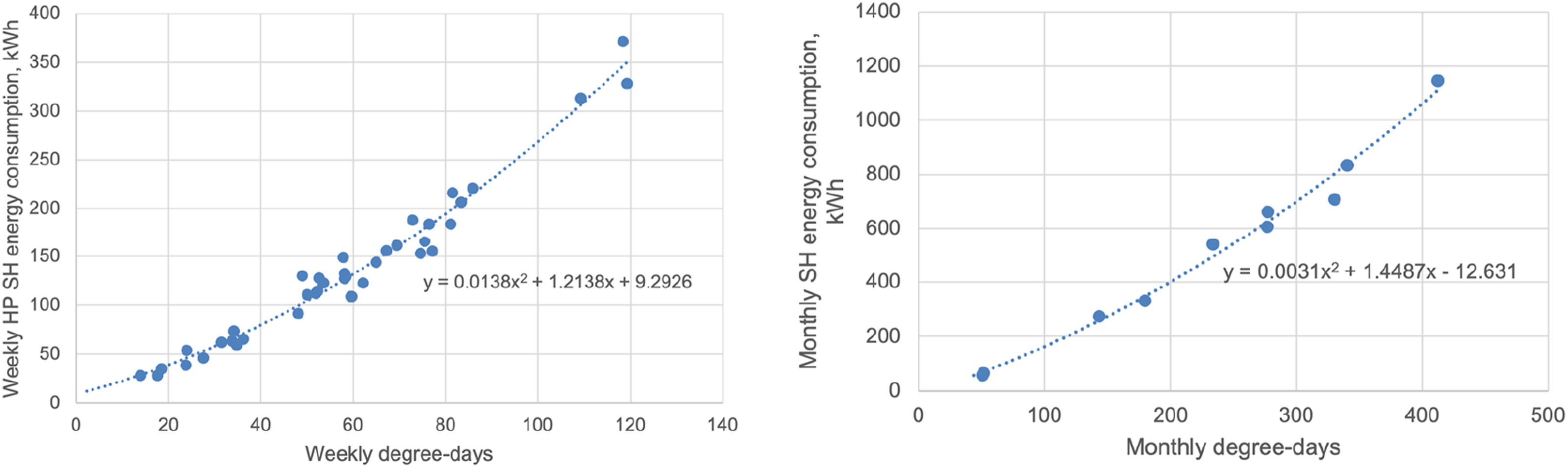
The heat pump was installed in March 2023, and included integrated electricity and heat metering, with separation of SH and DHW usage (these are never coincident and are easy to separate with this type of heat pump). Figure 6 shows daily heat pump space heating electricity consumption against daily degree-day to daily base temperatures for the period 17/3/23-4/4/24 (summer months removed). This result shows two key characteristics: the scatter is much reduced (R² = 0.9216) compared with the oil regime, and there is a marked curvature to the line of best fit, as shown by a second order polynomial fit. A simple linear fit would not fully characterise the data in this case (see below). The scatter reduces yet further for weekly and monthly aggregation (R² = 0.97 and 0.98 respectively), see Figure 7, and this indicates the heat pump has a more consistent control regime than for oil. The heat pump is set for continuous running with night set back, while the oil was timed for twice-daily operation.

Figure 6.

Daily space heating energy consumption against daily degree-days to daily base temperature, U′ = 371 W K⁻¹, SGF = 0.5, for the period 17/3/23-4/4/24.

Figure 7.

Weekly and monthly space heating energy consumption v degree-days, U′ = 371 W K⁻¹, SGF = 0.5, for the period 17/3/23-4/4/24.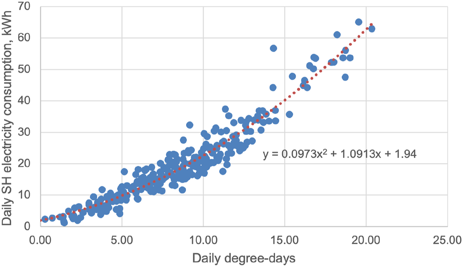

The observed curvature described by the polynomial fit is a key characteristic of heat pumps as the COP reduces during colder conditions (higher degree-days). This has the effect of increasing the energy consumption relative to the heat delivered, and simple linear regression should not be used for evaluating heat pump performance-in-use. This also means that HLC evaluations cannot be readily made using heat pump electricity consumption, unless weather adjusted COP is known across the operating range (an example is given at the end of this section). For fossil fuelled boilers the intra-seasonal variation in efficiency is across a smaller range (say 0.6 – 0.9) than is the COP for a heat pump (say 2.5 – 4). Linear regressions for fossil fuelled boilers may be more reliably used to characterise building energy performance, but this is certainly not the case for heat pumps, for which HLC evaluations require metered delivered space heating energy.

Figure 8 shows daily delivered space heating (no DHW) against daily degree-days to daily base temperature. For a daily regression the R² is remarkably high (0.8789) and good linearity is observed. In addition β is close to zero. These observations suggest the regression is reliable for the determination of the actual HLC. However, there is a caveat with this data. The raw data suggested that COPs in excess of 6 were being delivered on occasion, and indicated an HLC of around 500 W K⁻¹. Since the HLC of the house would not change due to a switch of heating system, this suggests the heat meter was over-estimating the system flow rates (the system flow and return temperatures were independently monitored and showed agreement with the heat pump measurements). The delivered heat values were scaled in accordance with the oil regime estimated HLC (346/500) to provide a starting point to optimise the regression and evaluate the house HLC. This arrived at a value of 371 W K⁻¹.

Figure 8.

Daily space heating delivered energy against daily degree-days to daily base temperature, U′ = 371 W K⁻¹, SGF = 0.5, for the period 17/3/23-4/4/24.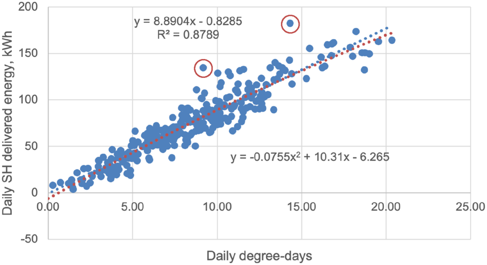

[Note: the two circled outliers in Figure 8 occurred during storm Isha in January 2024, with strong winds from the south-west. This shows an incidence of where the building HLC deviated markedly from its average value].

Table 4 shows the regression results produced for this property. This investigation explores the impact of choice of base temperature and timeframe aggregation. For each timeframe it can be observed that R² improves when using time-specific base temperatures when compared with using the overall average base temperature (17°C in this case). However, the slope values vary from ∼3% (daily) to ∼7% (monthly), which might be significant when selecting an HLC for forecasting future energy use. There is also an 11% difference between daily and monthly slopes, which would certainly be significant. These impacts will be explored when developing an energy predictor tool for assessing heat pump retrofit performance.

Table 4.

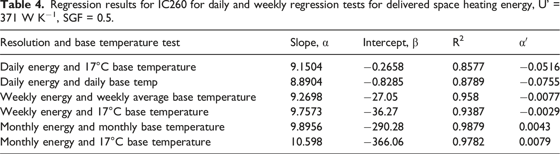
Regression results for IC260 for daily and weekly regression tests for delivered space heating energy, U’ = 371 W K⁻¹, SGF = 0.5.

Resolution and base temperature test	Slope, α	Intercept, β	R2	α′
Daily energy and 17°C base temperature	9.1504	−0.2658	0.8577	−0.0516
Daily energy and daily base temp	8.8904	−0.8285	0.8789	−0.0755
Weekly energy and weekly average base temperature	9.2698	−27.05	0.958	−0.0077
Weekly energy and 17°C base temperature	9.7573	−36.27	0.9387	−0.0029
Monthly energy and monthly base temperature	9.8956	−290.28	0.9879	0.0043
Monthly energy and 17°C base temperature	10.598	−366.06	0.9782	0.0079

The regressions shown in Figures 6 and 8 can be used to characterise the heat pump performance across the heating season by dividing the delivered energy by the energy consumed regression values for different degree-day values. This gives the weather adjusted COP that can be used for energy prediction and on-going system monitoring. The results are shown in Figure 9. The COP declines as the weather gets colder, as would be expected due to greater temperature gradients and defrost cycles. It is interesting to note how it also declines in warmer conditions. This is due to two factors. The first is that under extreme part load conditions the heat pump will cycle more often, leading to more start-up losses. The second is that the heat pump has continuous stand-by requirements to maintain the correct oil viscosity. This stand-by energy consumption is particularly apparent during the summer, when it averages around 0.6 kWh per day. These warm weather COPs occur in low energy use periods, and the impact on running costs are small.

Figure 9.

Heat pump COP v daily degree-days calculated from daily energy regressions.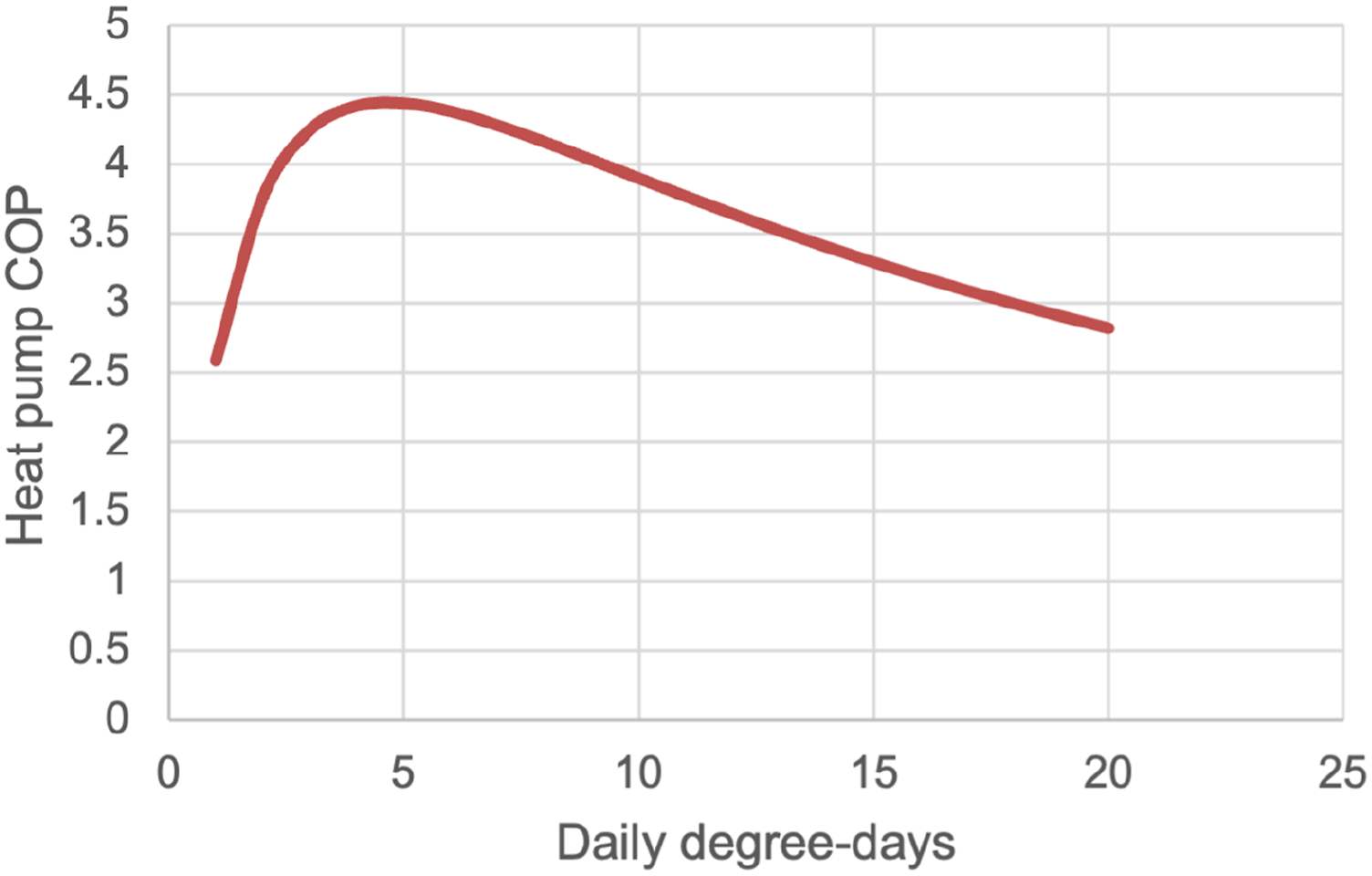

Conclusions

This paper has presented the results from two houses that have been extensively monitored to characterise their energy performance using a CIBSE TM41 methodology. The aim has been to show how regression analysis can be used to measure the real building heat loss coefficients using energy and environmental data, and how timeframe and data requirements can affect the results. The range of data variables and frequency of collection will strongly influence the cost and complexity of measurement and analysis, both of which need to be kept to a minimum for residential applications.

The examples presented here both show that regression slopes of delivered space heat against degree-days increase with longer timeframe aggregation (i.e. daily → weekly → monthly). These measured estimates of HLC can vary between 11% to 30% which has significant implications for the ability to establish an HLC. For many of the buildings studied the measured HLC was substantially different from that calculated from the site survey. This suggests that energy forecasting models should ideally use measured HLC values (rather than surveyed), and adopt the same analysis timeframe as that used to measure the HLC. As long as there is consistency between measurement and predictor timeframes then the method should be fairly robust.

For the retrofit of heat pumps there is the additional need to have reliable weather related COP characteristics. Again this needs to be applied with the same consideration to timeframe. Higher frequency modelling (e.g. daily) will require more detailed COP characteristics. This paper has presented a way to develop these for installed heat pumps. One specific finding of this work is that monitoring of heat pump energy use should adopt second order polynomial fits to characterise the operational performance.

The results of this work have implications for the amount (and cost) of data required for house energy analysis, and the level of complexity required to conduct this analysis and predict future system energy performance. These issues will be the subject of further work.