Producing domestic energy benchmarks using a large disaggregate stock model

Abstract

Within the UK, domestic buildings account for 16% of total national emissions. Considerable improvements to the performance of the existing building stock will be necessary in the context of the UK’s commitment to emissions reductions, and for this to be achieved successfully and efficiently will require an improved understanding of the current performance of the stock. This paper presents an analysis of metered gas and electricity use from 808,559 dwellings with detailed building characteristic data in London, showing how energy use can be examined using a highly detailed, fully disaggregate building stock model. New gas and electricity benchmarks have been produced for houses (split by the level of attachment) and flats, for both gas- and electrically-heated properties. The paper shows how energy use varies with form, and how the choice of units influences the relative performance of different types. Comparing gas use across the types, for example, when calculated as kWh/m², consumption follows building compactness, but when calculated as kWh/household, the trends follow building size. Finally, the paper examines how energy use varies with building thermal performance, using the Heat Loss Parameter (HLP), a standardised measure which accounts for thermal transfer through building envelopes as well as via air flow.

Practical Application: This paper presents domestic energy consumption benchmarks based on measured not modelled data, produced from a large sample of London houses and flats. Results are shown for different dwelling types and heating fuels. Additionally, the relationship between gas use and envelope thermal performance is explored. The results will hopefully be beneficial for researchers, policy-makers and designers interested in better understanding current domestic energy use, and informing decisions about future improvements to energy efficiency within the stock. This paper also provides details for anyone interested in the production of the domestic benchmarks for the CIBSE benchmarking tool.

Introduction and context

The UK domestic stock consists of 29 million homes, and is responsible for around 16% of national emissions. ¹ Considering London, the capital’s 1.5 million houses and 1.9 million flats ² together account for 55 TWh of energy use and 11MtCO₂e of emissions annually ³ (approximately 39% and 34% of the city’s totals). Since 1990 (the baseline normally used for national carbon reduction targets), building emissions have fallen, owing to changes in the stock itself as well as external factors such as a major drop in the carbon intensity of mains electricity. ¹ Reflecting the size of the domestic sector and its current condition, if the trends in carbon reduction are to successfully continue towards the target of Net Zero by 2050, significant improvement to UK housing will be necessary over the coming decades. This is likely to include envelope thermal performance measures, such as insulation, as well as a transition from heating primarily from fossil-fuels (predominantly gas boilers) to low carbon sources such as heat pumps. ¹ Any successful rollout of retrofits across such a large number of buildings and over a diminishing period of time will require an improved understanding of the stock; both in terms of its characteristics and make up, as well as its current performance.

The data available to investigate the building stock at an urban scale has changed dramatically over the past 10–15 years. ⁴ In the UK, more extensive detailed data is now available, enabling a greater understanding of the stock, plus a shift towards a more epidemiological approach to buildings research. ⁵ Building stock modelling, in particular with relation to energy use, is beginning to see a transition from sector-specific or archetype-based models, towards what was previously impossible over large areas; considering each building individually. Recent studies using data to undertake disaggregate modelling across large urban areas have included analyses of the current and potential performance of the school and domestic sectors,^6,7 and the quantification of potential for integrating rooftop photovoltaics. ⁸ Naturally, these changes are accompanied by increased complexity in data processing and analyses.

While the size of modern urban models generally remains small compared with typical quantitative measures of ‘big data’ in other scientific fields,^9,10 this still represents a shift in “how the data is organised …, how we tame it, store it, and process it, and what it tells us about the city.” ⁴ Within this context, this paper has two broad aims:

i. Methodologically, it provides a detailed overview of the production of domestic energy benchmarks using models of each individual building (rather than archetypes) using 3DStock, a highly detailed and disaggregate building stock model. More generally, this is how sources of buildings data, acting at different levels and originally produced for different purposes, can be used together within an urban-scale model. This will hopefully be of benefit to those developing – or working with outputs from – similar models. The paper expands on prior articles that have detailed the development of 3DStock,^2,11 and applied the model to building performance research.^12,13

ii. In terms of results, the paper improves the understanding of the current performance of domestic buildings, by analysing gas and electricity meter data for almost a million dwellings in London. The study accounts for different built forms and heating fuels, and explores the relationship between energy use and envelope thermal performance. The main benchmarks have been published on the CIBSE (Chartered Institution of Building Services Engineers) benchmarking tool, ¹⁴ a website that provides up-to-date energy performance information for building users and designers.

The remainder of the paper is structured as follows. Firstly, a brief literature review is provided. Next, the methodology introduces the data and details the steps to clean, process and combine the separate datasets. Next, the energy use results are presented and discussed. Finally, this work is part of longer-term research, so the conclusion includes a discussion of ongoing and planned work.

Domestic energy use in the UK

To date, considerable research has explored the performance of UK domestic buildings. This includes statistical analyses of large-scale disaggregate datasets, detailed surveys undertaken on small samples of buildings, as well as building simulation using various modelling approaches.

One of the most significant contemporary sources of information on domestic energy is NEED (the National Energy Efficiency Data-Framework), the government’s disaggregate stock model, that combines gas and electricity meter data with information on the national housing stock collected from various sources including energy efficiency schemes. ¹⁵ Each year, NEED reports summarise domestic energy use, including how demand varies with key building characteristics such as building age. ¹⁶ While access to NEED is restricted, ¹⁷ research has been undertaken using this data, or portions of it. Recent studies include: analyses of the relationship between energy and energy performance certificates (EPCs) in gas-heated houses ¹² ; and between domestic energy and urban morphology ¹³ ; analysis of the impact of various retrofits on performance ¹⁸ ; and comparison between the empirical data in NEED with modelled energy use. ¹⁹ Studies have also used aggregated outputs from NEED to assess the long-term improvement potential of the domestic stock ²⁰ and the relationship between energy and urban density ²¹ ; used a precursor to NEED to assess how domestic energy use varies with physical and social factors^22,23; to track the uptake of improvements across the stock ²⁴ ; and evaluate the representativeness of some of its underlying data. ²⁵

While the studies described above evaluated annual energy consumption data, studies have also made use of high-resolution smart meter and sub-meter data. During 2010–11, the Household Electricity Survey (HES) monitored total and appliance-level electricity in 250 English households. ²⁶ While the sample size is far smaller than the NEED-based studies, the use of smart meter data enabled factors like daily demand profiles and base loads to be assessed for specific appliances and electric heating. ²⁷ Elsewhere, smart meter data from 780 UK homes was used to examine the relationship between external temperature and heating, ²⁸ and several years of electricity data for 5567 London dwellings was used to explore the impact of dynamic tariffs on energy use.^29,30 Finally, at a still larger scale, the ongoing SERL (Smart Energy Research Lab) project is collecting half-hourly and daily electricity and gas use data for over 13,000 homes. ³¹ This data is available for research purposes, and has been used to explore how domestic energy relates to variables from EPCs and household questionnaires. ³²

Alongside NEED, there are several other long-running documents on UK housing characteristics. Most notably EHS (the English Housing Survey) and EFUS (the Energy Follow Up Survey). ³³ Running since 1967, EHS is an annual survey of “people’s housing circumstances and the condition and energy efficiency of housing in England.” ³⁴ It gathers information on the physical characteristics, internal systems, and demographics of the stock each year through building surveys and household interviews across thousands of dwellings. EHS was a source of information for the Housing Energy Fact File, published from the 1990s until 2013, to provide an overview of UK housing, covering issues including performance, construction and coverage of efficiency measures. ³⁵ EHS is also a crucial source of data for modelling and is used in models of domestic energy, ³⁶ overheating risk^37,38 and fuel poverty. ³⁹ Perhaps most notably for energy, EHS forms the backbone of the National Household Model (NHM),^40,41 and its precursor, the Cambridge Housing Model (CHM). ⁴² While NHM/CHM are steady-state, monthly energy models, EHS is also used as input data for dynamic simulation.^43,44

The CIBSE benchmarking tool

The CIBSE Benchmarking Tool was developed in collaboration between CIBSE and UCL (University College London), with an aim to support the UK’s transition towards the 2050 Net Zero target. ¹⁴ The tool is a free and publicly accessible online platform that provides up-to-date, reliable and relevant performance data for designers, users and other stakeholders in the built environment. Energy use intensity benchmarks are presented, including typical and good practice figures, based on analyses of empirical data rather than modelled performance.

At the time of writing, the tool presents a mix of existing benchmarks from CIBSE Guide F ⁴⁵ alongside new benchmarks produced from analyses of large-scale data including the Display Energy Certificates database. ⁴⁶ Results are presented for a range of building types including education, healthcare and hospitality buildings, as well as the domestic typologies from the present paper; work is ongoing to further expand the coverage, including several commercial building uses. Alongside expanding the types of buildings covered over time, the tool has also been designed to be a framework that can evolve, allowing incorporation of new methods of data collection, such as crowdsourcing. By making use of big data from across the built environment, the tool will eventually provide contextualised benchmarks that reflect the latest trends in energy use across a wide range of domestic and non-domestic building types. ¹

Methodology

This study uses data from three main sources:

- 3DStock: 3DStock is a disaggregate stock model covering domestic, non-domestic and mixed-use buildings across very large urban areas. Built using data from sources including OS (Ordnance Survey), the Environment Agency and the VOA (Valuation Office Agency) the model includes highly detailed information on the physical form and characteristics of the built environment. Within the model, each property is fully addressed and geo-located. This means that property-level data can be individually address-matched (e.g. energy meters for each flat in a block), while aggregate data can be spatially matched (e.g. census demographics). To date, 3DStock models have been produced for several regions in Britain, including London and all of Wales. Readers looking for more information on the model may refer to papers detailing its development,^2,11 or its application to a wide range of research.^{12,13,21,47–51} A version of 3DStock for London has been created for the GLA (Greater London Authority) called LBSM (the London Building Stock Model), which is freely available online and allows the model to be interrogated through a simple webmap. ⁵² The 3DStock model used in this study covers all of London, and is a snapshot for 2017.

- Gas and electricity meter data: Annual electricity and gas meter data for London have been released to the team by BEIS (the Department for Business, Energy and Industrial Strategy). This was provided for undertaking research for BEIS, under strict confidentiality and security measures. The energy data used in this study covers the year 2016.

- Domestic EPC (Energy Performance Certificates) data: EPCs provide information on the characteristics of buildings along with their current and potential predicted performance for prospective buyers or tenants. ⁵³ The A-G grades, which represent normalised ratings based on modelled energy costs and emissions are a dominant feature of EPCs. For this study, however, these modelled outputs are not used, since the actual meter data are available; instead, EPCs have been used as a source of information on the characteristics of each property. Bulk EPC data has been published online since 2017, and this study uses EPCs lodged until mid-2020.

Considerable work was required to process and combine the data from the three sources, as outlined in Figure 1. Broadly speaking, 3DStock was used as a central ‘spine’ (step A1) onto which energy and EPC data were attached (steps B1-B4). After the data-matching was complete, the overall information available for each dwelling was checked, and any homes with inconsistent, questionable, or incomplete data were excluded (step C1). These steps are detailed below, after some key concepts are introduced.

Figure 1.

Overview of the data processing.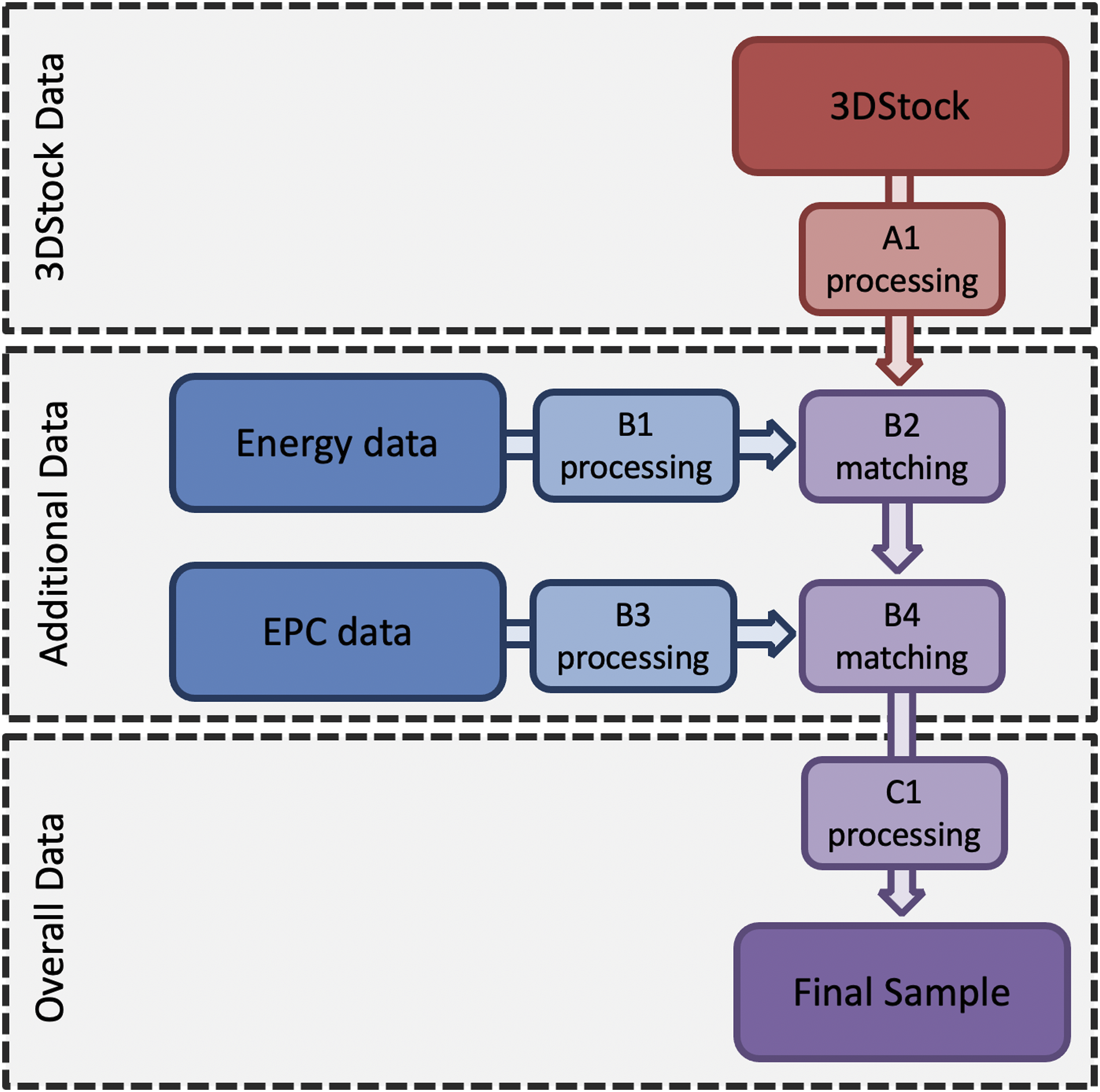

Terminology and scope

The paper, so far, refers to ‘buildings’ and ‘dwellings.’ However, strictly speaking, 3DStock is built around ‘SCUs’ (Self Contained Units) and ‘UPRNs’ (Unique Property Reference Numbers). The distinction between buildings and SCUs is largely technical, to ensure clean attribution of data in complex built forms; the key idea is that no premises should be split across multiple SCUs. ⁵⁴ For example, two neighbouring terrace houses would be separate SCUs. However, if they were converted so that the ground floor became one large shop with flats above, this would now be considered a single SCU to not ‘split’ the shop. UPRNs are unique identifiers for each address in Britain. Multi-occupant buildings can also have a ‘parent UPRN’ for the building shell. Thus, in the example, the original terrace houses would be separate SCUs each having a single domestic UPRN, while the conversion would be a single SCU, with a parent UPRN, a non-domestic UPRN and multiple domestic UPRNs, representing the building shell, shop, and flats respectively. In practice, for much of the stock (except for particularly complex arrangements typically in the non-domestic sector), SCUs and UPRNs are analogous to ‘buildings’ and ‘premises’ respectively.

For this study, the analysis has been limited to purely domestic SCUs; that is houses, and blocks of flats without non-domestic premises (so flats-above-shops, e.g., are excluded). Within London, 79.6% of blocks of flats are purely domestic, and 77.3% of all flats are in purely domestic buildings. ⁴⁹ Under this scope, the building types are therefore defined as follows:

- Houses: Single SCUs, each with a single domestic UPRN.

- Flats: Single SCUs, each with one UPRN per flat. Most also have a parent UPRN for the building.

Reflecting the available meter data, the analysis is restricted to gas-heated and electrically-heated dwellings. Households served by other fuels (e.g. oil) or connected to large district/community energy schemes supplying multiple buildings are excluded. The former because the energy data is unavailable, and the latter because it is not currently feasible to reliably attribute specific buildings to specific networks. Note that the meter data does not record exported electricity, so the impact of on-site renewables (such as rooftop photovoltaics) will only be observed where these reduce electricity demand. Similarly, the proportion of energy used outside the building, such as for electric vehicles, is also unknown. However, for 2016–17, these would have accounted for a small percentage of London households.

Steps A1-C1

The following sub-sections detail the data processing and combination steps.

Step A1: processing 3DStock

Reflecting the scale and complexity of 3DStock, there are instances of errors, inconsistencies, and data gaps within the model. This can occur where, for example, two pieces of input data were originally collected at different times, and a building changed significantly in the intervening period. Any SCUs with such issues were excluded. Non-domestic and mixed-use blocks were also excluded, reflecting the project scope. Following this, the sample included 1,516,730 houses (representing 97.9% of all London houses), and 1,345,409 flats across 279,846 blocks (88.3% and 94.4% of the purely domestic stock respectively).

Steps B1-B4: adding energy and EPC data

Processing was undertaken on the meter data before matching to 3DStock (step B1). Within the raw energy data, a small number of meters have multiple readings in a single year or have NULL readings. The former were summed to produce a total annual consumption per meter, and the latter were removed. Energy analyses typically exclude meters with readings beyond certain limits as part of pre-processing. ⁵⁵ Here, thresholds were applied on the basis of annual energy use intensities (kWh/m²) instead.

Next, meters were address-matched to the 3DStock addresses (step B2). The raw energy data consists of separate files for gas and electricity, so these were processed independently. Levenshtein distance was used for address-matching quality assessment, with a minimum ratio of 0.75 applied. ²

Considerable processing of the raw EPC data was necessary (step B3). Given the focus of the study on energy, the following key fields were tidied and parsed: main_fuel, mainheat_description, secondheat_description, hotwater_description. The plant and fuel type(s) were identified from the data, as well as instances of connections to communal heating systems. A three-letter code was generated for each dwelling, representing the fuel listed for (i) primary space heating, (ii) secondary space heating and (iii) water heating. Thus, ‘GGG’ represents a dwelling with gas for all three uses, while ‘G-E’ represents a dwelling with gas primary heating, no secondary heating, and electric water heating. Entries with errors or internal inconsistencies, or where data was missing or too vague to parse were excluded (e.g. heating system listed as ‘boiler’ without the fuel). EPCs were also used as the source for dwelling size (floor area and number of rooms), and dwelling type was taken from the EPCs in conjunction with 3DStock.

As with the energy data, address-matching was carried out between the EPCs and 3DStock (step B4). Where a dwelling had multiple EPCs, the one lodged closest to 2017 (the model year) was selected.

Step C1: processing the combined data

Finally, the overall data for each dwelling was checked for internal consistency and to apply general data requirements (step C1). A key issue to resolve was to be confident that the meters matched to each dwelling accurately reflect its energy use. For example, 4.3% of the houses have no matched gas meter. However, this will include data errors (e.g. where the address-matching has failed), as well as houses without gas heating.

Several stages of checks were carried out, using the meter and EPC data, to produce an overall confidence grade for each dwelling, as detailed below.

Metering arrangements

Figure 2 illustrates typical energy supply arrangements for houses and blocks of flats in London. ³ The green and red lines represent electricity and gas supplies respectively, and the solid circles represent the meters (for which consumption figures are available). The dashed lines represent distribution within buildings downstream of the meters (electricity/gas/heat), for which disaggregate consumption data is unavailable.

Figure 2.

Typical electricity and gas supplies for dwellings in London.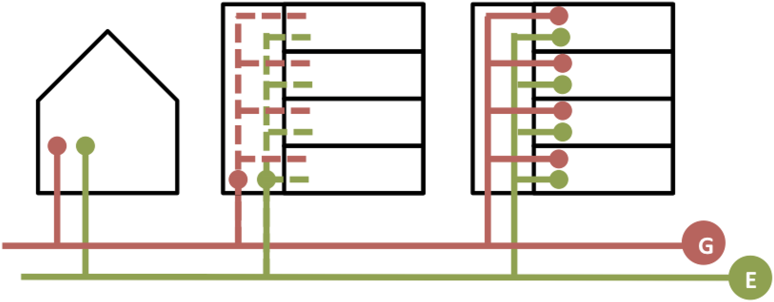

For houses (Figure 2, left), the arrangement is generally straightforward: Each house typically has its own electricity and, possibly, gas supply with associated meter(s). Other arrangements, such as houses with multiple gas meters or no electricity meters, may exist, but are uncommon and were assumed to be more likely to represent errors or district systems. Table 1 summarises the different meter arrangements in houses, how each was treated, and the proportion of the London stock this covers. ⁴ Note that, since overall data confidence can only be fully determined based on the meter and building systems data, dwellings with ‘poor’ confidence grades were identified at this stage but not ‘good.’

Table 1.

Meter arrangements for London houses.

Ref	No. meters matched to house		Process		% Of houses
	Gas	Electricity	Assumption	Grade
H1	1	1	Gas-heated house	-	91.7%
H2	0	1	Possibly all-elec house	-	3.2%
H3	Any count	0	Unlikely	Poor	2.6%
H4	>1	Any count	Unlikely	Poor	1.2%
H5	Any count	>1	Unlikely	Poor	1.6%
H6	Any count	Landlord meters	Unlikely	Poor	0.1%

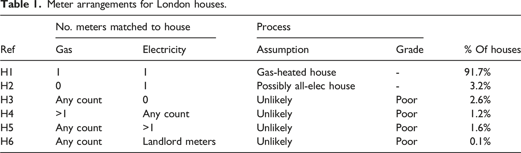
The table shows that 91.7% of London houses have one gas and one electricity meter matched (ref H1), while 3.2% have only a single electricity meter (H2). A small proportion of electricity meter addresses refer to landlord spaces (H6). Following this process, the gas and electricity use for each house was calculated from the matched meters.

In contrast to houses, the process for flats was considerably more complicated. Gas and electricity can feasibly be supplied to individual flats (Figure 2, right) or to the block (Figure 2, middle), or a combination of the two (e.g. electricity to each flat, but a central gas boiler serving the block). Theoretically, this should be reflected within the data: for blocks where utilities serve individual flats, the meters should address-match to the UPRNs (i.e. to each dwelling), and for those where utilities serve the block, the meters should address-match to the parent UPRN (i.e. the overall block). However, processing errors could result in meters for flats being matched to the overall block or to different flats in the same block (flats within a block typically have nearly identical address strings, making address-matching difficult). Furthermore, blocks may have additional meter(s) serving shared/landlord spaces and equipment. This means that the energy use for a flat may come from the meters address-matched to that flat and/or a portion of the meters matched to the overall block, and a portion of the meters serving shared/landlord spaces.

For these reasons, checks on the energy data for flats were undertaken at two scales: for each individual flat first, and then for the overall block. These are outlined in Table 2 and Table 3 respectively.

Table 2.

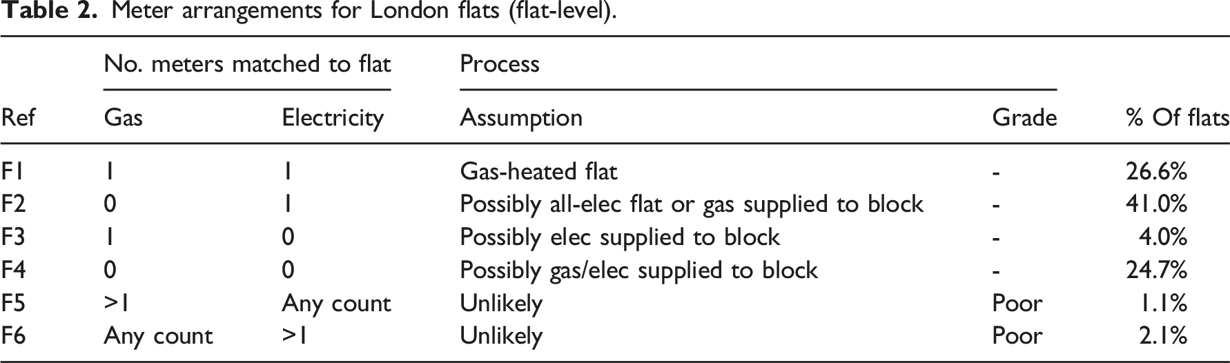
Meter arrangements for London flats (flat-level).

Ref	No. meters matched to flat		Process		% Of flats
	Gas	Electricity	Assumption	Grade
F1	1	1	Gas-heated flat	-	26.6%
F2	0	1	Possibly all-elec flat or gas supplied to block	-	41.0%
F3	1	0	Possibly elec supplied to block	-	4.0%
F4	0	0	Possibly gas/elec supplied to block	-	24.7%
F5	>1	Any count	Unlikely	Poor	1.1%
F6	Any count	>1	Unlikely	Poor	2.1%

Table 3.

Meter arrangements for London flats (block-level).

Ref	No. meters matched…				Process	Gas				Electricity
	… to Flat	… to block	… total	Assumption	Energy calculation approach	% flats	% blocks	Grade	% flats	% blocks	Grade
B1	Mf = 0	Mb = 0	Mf + Mb = 0	No energy or district system.	-	18.6	9.8	-	3.4	3.2	Poor
B2	0 < Mf < F	Mb = 0	0 < Mf + Mb < F	Energy supplies each flat. Flats w/out meters either have no supply (e.g. no gas) or are missing meters.	Disaggregate: Each flat assigned matched energy where available	14.7	13.7	-	22.4	15.2	-
B3	Mf = F	Mb = 0	Mf + Mb = F	Energy supplies each flat.	Disaggregate: Each flat assigned matched energy	23.1	40.2	-	35.9	45.6	-
B4	Mf > F	Mb = 0	Mf + Mb > F	Meter errors for flats.	-	0.0	0.0	Poor	0.0	0.0	Poor
B5	Mf = 0	Mb > 0	0 < Mf + Mb < F	Possibly a mix of unusual metering and/or poor address-matching.	Aggregate: All flats assigned a share of total energy use	17.1	10.3	Poor	6.1	6.7	Poor
B6	0 < Mf < F	Mb > 0	0 < Mf + Mb < F	Possibly a mix of unusual metering and/or poor address-matching.	Aggregate: All flats assigned a share of total energy use	5.0	2.3	Poor	7.4	2.6	Poor
B7	Mf = 0	Mb > 0	Mf + Mb = F	Energy supplies each flat, but meters are not address-matched.	Aggregate: All flats assigned a share of total energy use	14.2	15.5	-	6.8	12.2	-
B8	0 < Mf < F	Mb > 0	Mf + Mb = F	Energy supplies each flat, but some meters have only matched to block.	Disaggregate: Flats with meters assigned matched energy. Aggregate: Flats w/out meters assigned share of the energy matched to the block.	4.2	5.8	-	7.8	8.1	-
B9	Mf = 0	Mb > 0	Mf + Mb > F	Possibly a mix of unusual metering and/or poor address-matching.	Aggregate: All flats assigned a share of total energy use	2.0	1.3	Poor	1.3	1.7	Poor
B10	0 < Mf < F	Mb > 0	Mf + Mb > F	Possibly a mix of unusual metering and/or poor address-matching.	Aggregate: All flats assigned a share of total energy use	0.8	0.6	Poor	3.9	2.0	Poor
B11	Mf = F	Mb > 0	Mf + Mb > F	Energy supplies each flat. Energy to block supplies circulation/shared areas.	Disaggregate: Each flat assigned matched energy PLUS a portion of the energy matched to the block	0.4	0.5	-	5.0	2.7	-
B12	Mf > F	Mb > 0	Mf + Mb > F	Meter errors for flats.	-	0.0	0.0	Poor	0.0	0.0	Poor

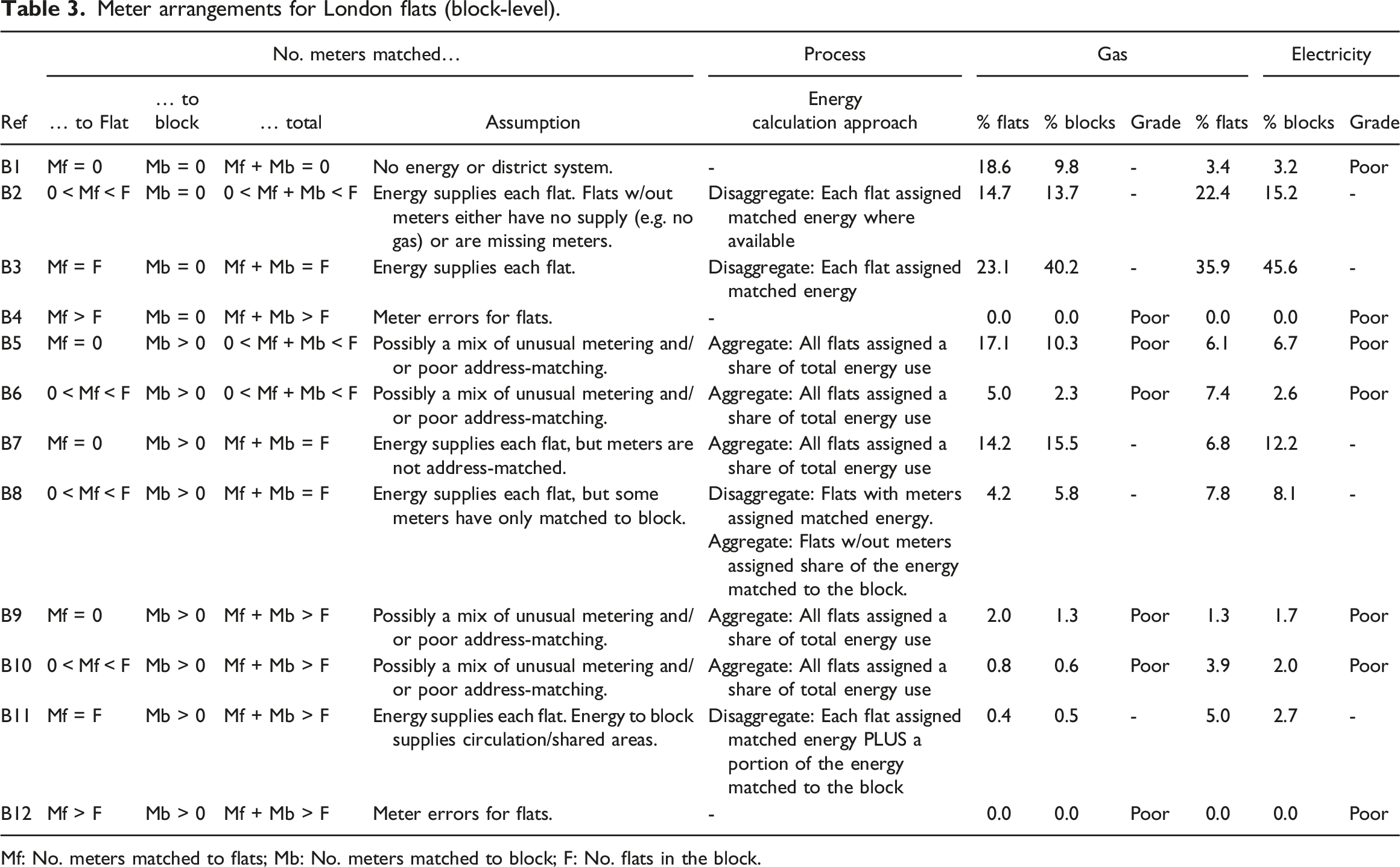
Mf: No. meters matched to flats; Mb: No. meters matched to block; F: No. flats in the block.

The flat-level checks were similar to those for houses, except any energy for landlord meters was distributed across all flats in the block. The results show that a quarter of flats have single gas and electricity meters matched (ref F1), while a further 41% have just a single electricity meter matched (F2).

For the block-level checks, comparison was made between the total number of meters (matched to individual flats or the block), and the number of flats. This comparison was made separately for gas and electricity. Example arrangements from Table 3 are explained below:

- Ref B1 shows that 9.8% of blocks (representing 18.6% of flats) have no matched gas meters, and 3.2% of blocks (representing 3.4% of flats) have no electricity meters. The former cases are potentially electrically-heated blocks, while the latter were assumed to be unlikely and assigned ‘poor’ confidence grades.

- Ref B3 shows that, in 40.2% of blocks, every flat has a gas meter with no gas meters matched to the block itself. For electricity meters this is 45.6% of blocks. In this case, the energy use for each flat is calculated directly from the meter matched to it.

- Finally, ref B8 shows that in 5.8% of blocks, the number of gas meters matched to the flats plus the number of gas meters matched to the block equals the number of flats (for electricity meters the result is 8.1%). In this case it is assumed that the true metering arrangement is the same as the previous example (i.e. the meters matched to the block represent address-matching issues). Therefore, the energy use for each flat is calculated from the matched meters where available, while flats without matched meters are given an average kWh/flat calculated from the sum of the meters matched to the block.

Meters and EPC data

The raw electricity meter data includes the profile classes. Economy 7 (profile class 2) is a tariff that provides cheaper electricity during off-peak hours, and is associated with electric heating. ²³ However, within the sample, 86.9% of London houses with Economy 7 m also have gas meters, and the typical gas and electricity use profiles of such houses are similar to those for houses on other electricity tariffs. Consequently, the profile class was not considered a reliable means of identifying electrically-heated properties. Comparison was instead made between the energy data and the systems identified from the EPCs.

Households were given ‘Poor’ confidence grades if no gas meter was matched but the EPC listed gas use for space or water heating. Conversely, if gas meters were matched, but the EPC listed no gas use this could feasibly represent gas cooking, so ‘Okay’ grades were given. ⁵ Dwellings where the EPC listed any fuel except gas/electricity for space or water heating were given ‘Poor’ grades, since consumption data for these fuels was unavailable. Similarly, EPCs which listed communal systems were given ‘Okay’ ratings, since the energy consumption of those dwellings would only be available at an aggregate level. Finally, dwellings without matched EPCs were given a ‘Poor’ grade (at the time of writing around half of London dwellings).

Final energy sample

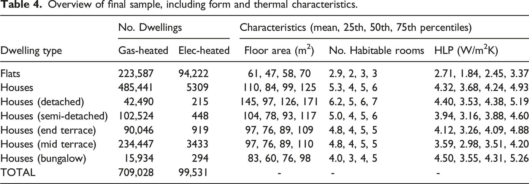
Following the above steps, the final sample of dwellings was selected to ensure only dwellings were included with disaggregate electricity and (where applicable) gas meter data, appropriate space and water heating systems, and reasonable values for size and energy consumption. These were selected on the following basis:

- Good meter data: excludes dwellings assigned ‘poor’ or ‘okay’ grades during the meter processing.

- Disaggregate energy: excludes flats for which meters were only available (or could only be matched) at a block level.

- Good EPC data: excludes dwellings assigned ‘poor’ or ‘okay’ grades during the EPC processing.

- Systems: excludes dwellings with a mix of fuels listed in the EPC data (e.g. gas space heating and electric water heating). Using the codes defined during step B3, only the following were included: GGG or G-G for gas-heated properties, and EEE or E-E for electrically-heated properties.

- Area and energy thresholds: excludes dwellings with size or energy intensities outside of the following limits: 10–1,000 m² and 5–500kWh/m².

Following this process, the final sample consists of 808,559 dwellings, summarised in Table 4. This represents 32% of all houses in London, and 21% of flats in domestic blocks (or 16% of flats). For each property, information on the dwelling type, total floor area, fuel uses and annual gas and electricity meter data are known. Additionally, the number of habitable rooms ⁶ is available via the EPCs for most dwellings. Within the data, 0.3% of dwellings in the final sample lack room counts. (The floor area, dwelling type and energy data have complete coverage.) The mean and quartile values for form are included for each dwelling type in Table 4.

Table 4.

Overview of final sample, including form and thermal characteristics.

Dwelling type	No. Dwellings		Characteristics (mean, 25th, 50th, 75th percentiles)
	Gas-heated	Elec-heated	Floor area (m2)	No. Habitable rooms	HLP (W/m2K)
Flats	223,587	94,222	61, 47, 58, 70	2.9, 2, 3, 3	2.71, 1.84, 2.45, 3.37
Houses	485,441	5309	110, 84, 99, 125	5.3, 4, 5, 6	4.32, 3.68, 4.24, 4.93
Houses (detached)	42,490	215	145, 97, 126, 171	6.2, 5, 6, 7	4.40, 3.53, 4.38, 5.19
Houses (semi-detached)	102,524	448	104, 78, 93, 117	5.0, 4, 5, 6	3.94, 3.16, 3.88, 4.60
Houses (end terrace)	90,046	919	97, 76, 89, 109	4.8, 4, 5, 5	4.12, 3.26, 4.09, 4.88
Houses (mid terrace)	234,447	3433	97, 76, 89, 110	4.8, 4, 5, 5	3.59, 2.98, 3.51, 4.20
Houses (bungalow)	15,934	294	83, 60, 76, 98	4.0, 3, 4, 5	4.50, 3.55, 4.31, 5.26
TOTAL	709,028	99,531	-	-	-

Building thermal performance

While the main aim of this paper is the production of domestic energy benchmarks, work was also undertaken to quantify how energy use varies with building thermal performance. For this, the HLP (Heat Loss Parameter) was calculated for each dwelling. HLP is a measure of a building’s overall heat loss, normalised by floor area to allow comparison between different building forms and sizes. It accounts for thermal transfer through the building envelope and via air flow, and is measured in units of W/m²K. Since HLP is not provided directly within the EPC data release, it was calculated using equations 26–40 from the SAP methodology. ⁵⁶ Input data on the envelope characteristics and form came from EPCs and 3DStock. For example, wall U-values were estimated using the EPC wall_description and construction_age_band fields in conjunction with Table S6, ⁵⁶ while the associated envelope areas were provided by 3DStock. Since data on the number of vents (e.g. chimneys) is currently unavailable at a disaggregate level through any of the sources, overall mean counts for each dwelling type-age band combination were used, from London data. ⁵⁷

For some of the sample dwellings, HLP could not be estimated reliably. This includes instances where the information within the EPCs is too vague to parse, where multi-type construction elements were listed (e.g. a house with solid walls plus cavity walls, since their proportions cannot currently be calculated), or where the 3DStock physical form data was unreliable, resulting in either no HLP result, or very high/low values. From the overall sample, HLP could not be calculated for 0.1% of dwellings, while a further 0.1% of houses and 1.7% of flats were excluded from this portion of the analyses for HLP results outside of the range 1–10 W/m²K. Summary HLP values are included in Table 4. At the time of writing, there is no alternative source of large scale disaggregate form data for London housing for comparison. However, the figures from 3DStock align closely against those calculated from the EHS sample for London ⁵⁷ : detached, semi-detached, mid-terrace, end-terrace houses and flats have differences in median HLP between EHS and 3DStock of +5%, +8%, +15%, +6% and −3% respectively, while the same figures for median floor area are −12%, −3%, +2%, +4% and −1%.

Results and discussion

In line with the CIBSE benchmarking tool, ¹⁴ energy performance is presented here as cumulative distribution curves. A table of key values is also provided, including ‘typical’ and ‘good practice’ benchmarks (the 50th and 25th percentiles respectively). Where appropriate, tests have been undertaken to explore whether differences are statistically significant. Energy consumption data are non-normal, so Mann–Whitney–Wilcoxon tests (MWW) have been used when analysing pairs of variables (e.g. comparing gas-heated and electrically-heated dwellings), while Kruskal–Wallis tests (KW) followed by Dunn’s test with a Bonferroni adjustment to the p-value have been used for larger numbers of variables (e.g. comparing dwelling types).

Overall energy benchmarks

Figure 3 shows the annual energy use intensity profiles, in terms of kWh/m², for each dwelling type. Figure 3(a)–(c) show gas, electricity and total energy use respectively for gas-heated dwellings, while Figure 3(d) shows electricity use for electrically-heated dwellings. The sample sizes are in brackets in the legend. Table 5 summarises the key results. It should be noted that the sample sizes for electrically-heated bungalows and detached and semi-detached houses are low, so these results should be treated with some caution.

Figure 3.

Annual energy use (kWh/m²) profiles for (a) gas, (b) electricity, and (c) total energy use in gas-heated dwellings, and (d) electricity use in electrically-heated dwellings.

Table 5.

Summary results for dwelling performance (kWh/m²).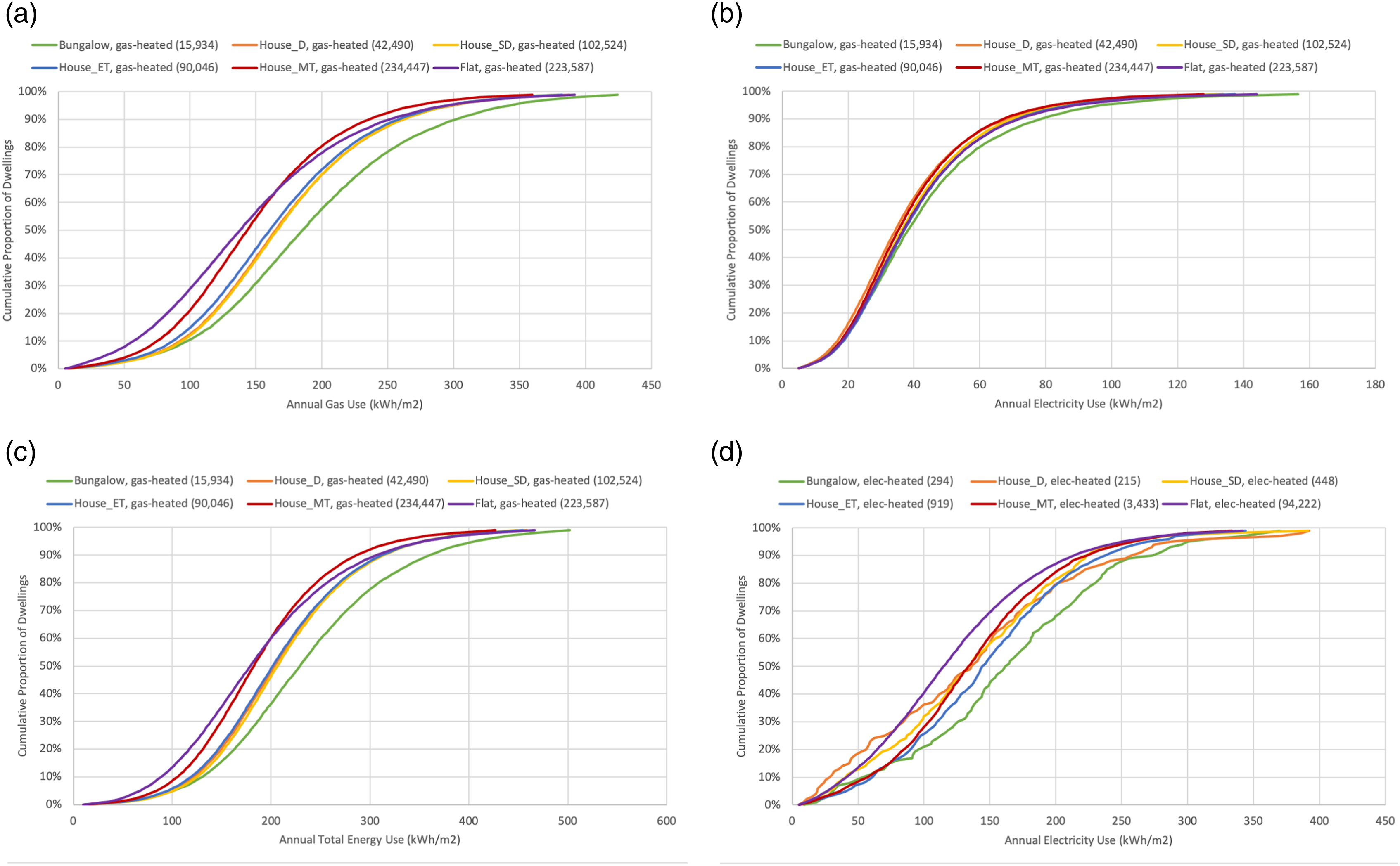

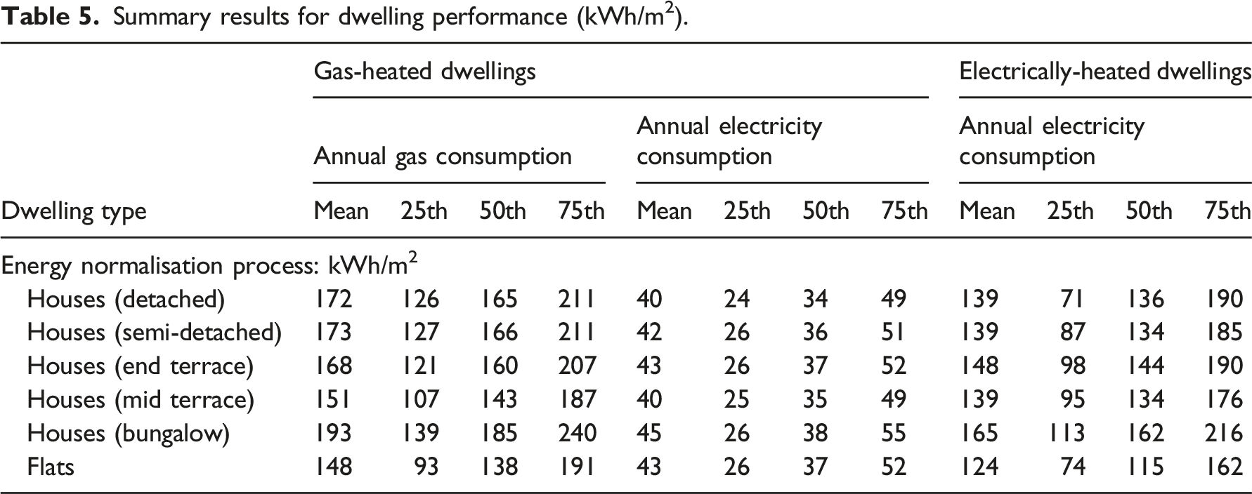
Dwelling type	Gas-heated dwellings								Electrically-heated dwellings
	Annual gas consumption				Annual electricity consumption				Annual electricity consumption
	Mean	25th	50th	75th	Mean	25th	50th	75th	Mean	25th	50th	75th
Energy normalisation process: kWh/m2
Houses (detached)	172	126	165	211	40	24	34	49	139	71	136	190
Houses (semi-detached)	173	127	166	211	42	26	36	51	139	87	134	185
Houses (end terrace)	168	121	160	207	43	26	37	52	148	98	144	190
Houses (mid terrace)	151	107	143	187	40	25	35	49	139	95	134	176
Houses (bungalow)	193	139	185	240	45	26	38	55	165	113	162	216
Flats	148	93	138	191	43	26	37	52	124	74	115	162

The results reveal the current performance of the sample domestic stock. In gas-heated dwellings, gas use remains higher than electricity. Median gas use in houses and flats are 154 and 138 kWh/m² respectively, compared with 36 and 37 kWh/m² electricity use (MWW, p < .01 between gas-heated houses and flats, for both gas and electricity). Across the dwelling types, gas broadly follows form. More compact types (flats and mid-terrace houses) show lower consumption than less compact forms (bungalows and detached houses), likely reflecting differences in heat loss through the envelope (KW, p < .01 for gas use in gas-heated dwellings). The post-hoc Dunn tests show that each of the pairs of dwelling types have statistically different gas consumption, except between detached and semi-detached houses. In contrast, the electricity profiles for gas-heated dwellings show far less variation between the types. While overall differences are still observed (KW, p < .01 for electricity use in gas-heated dwellings), and the Dunn tests show differences across each of the types, the magnitude of the differences is greatly reduced. Median gas use, for example, varies by 35% between the highest and lowest dwelling types, compared to only 11% for electricity use.

As may be expected, the electricity use profiles for electrically-heated dwellings more closely resemble gas-heated dwellings’ gas use than electricity trends, with 41% variation across the median electricity intensities (MWW, p < .01 between electrically-heated houses and flats). The trend with compactness is less clear-cut (e.g. detached houses have a relatively low median use amongst the electrically-heated types), but the smaller sample sizes for houses mean that this should be treated with caution (30% of flats in the sample have electric-heating, as-compared-with only 1% of houses). ⁷ Differences in energy use in electrically-heated dwellings are observed (KW, p < .01) but considering the breakdown, some pairs (detached houses and flats; end-terrace and bungalows; mid-terrace and detached houses; and semi-detached houses and detached, end-terrace and mid-terraced houses) are found to not be statistically significantly different.

Considering total energy, the results suggest this is lower in electrically-heated dwellings than gas-heated dwellings across all typologies (MWW, p < .01 between gas- and electric-heating for all types). Median total energy intensities are 29% and 36% lower in houses and flats respectively. It should be noted that, despite the lower total energy consumption, when the price of electricity is sufficiently higher than gas the associated median total annual energy costs will be higher for electrically-heated dwellings than gas-heated ones. ⁸ The differences in energy will partly reflect technical factors (typical gas boiler efficiencies within SAP are ∼60%–84%, compared with 100% for direct electric heating). ⁵⁶ Naturally, while heat pumps are still uncommon within UK domestic buildings, any large rollout (e.g. as part of the transition towards the national emissions reduction targets) should see a dramatic change in the energy profiles of the electrically-heated stock. Underlying differences in the characteristics of homes and households with different fuels will also indirectly influence energy. For example, electric-heating is associated with more recent constructions, and lower mean floor areas and HLP values in the sample (variables that directly impact on thermal performance), and nationally with lower income households and higher incidences of fuel poverty ⁵⁸ (factors that impact on the sensitivity to differences in price between gas and electricity).

Alternative energy normalisation approaches

A floor area-based approach to energy normalisation is used in historic benchmarking, ⁵⁹ assessment scheme methodologies^56,60 as well as proposed future design targets for transitioning towards Net Zero.^61,62 However, it has been shown that the choice of normalisation denominator can influence the apparent relative performance of the stock, since the distribution of building characteristics is often not uniform. 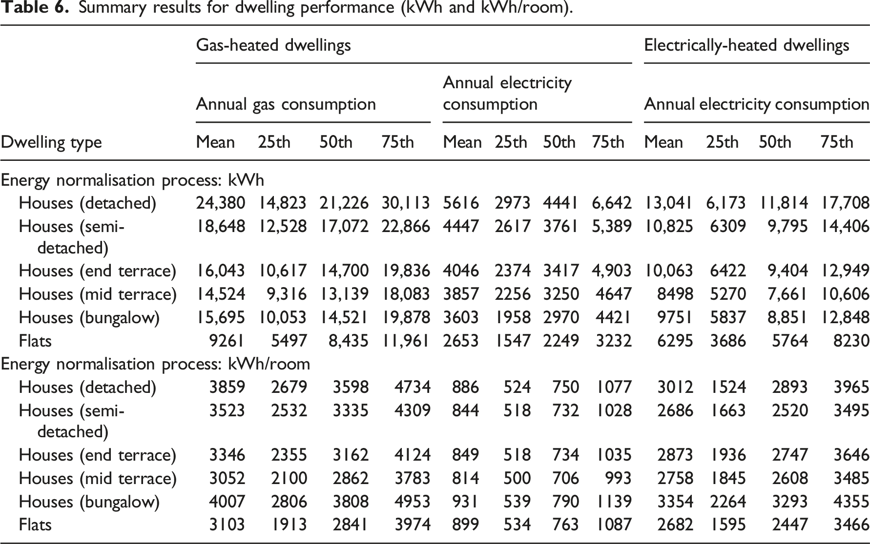⁶³ For the domestic sector, there are differences in typical size with type; for example, within the sample, median floor area for detached houses is double that for flats. Therefore, the benchmark plots are reproduced in terms of kWh (essentially kWh/household) and kWh/room, in Figure 4(a)–(d) and Figure 5(a)–(d), respectively. As noted, the sample sizes for the per-room results are slightly reduced, reflecting the available data. The results are summarised in Table 6. Comparing these energy consumption (kWh) values against 2016 household data for London from NEED reveals strong agreement: ⁶⁴ The difference in mean gas use for detached, semi-detached, end-terrace, mid-terrace houses and flats are −4%, −1%, +2%, +2%, −5% and +4% respectively, while the equivalent values for electricity use are −1%, +2%, +2%, +1%, −4% and +10% respectively. ⁹

Figure 4.

Annual energy use (kWh) profiles for (a) gas, (b) electricity, and (c) total energy use in gas-heated dwellings, and (d) electricity use in electrically-heated dwellings.

Figure 5.

Annual energy use (kWh/room) profiles for (a) gas, (b) electricity, and (c) total energy use in gas-heated dwellings, and (d) electricity use in electrically-heated dwellings.

Table 6.

Summary results for dwelling performance (kWh and kWh/room).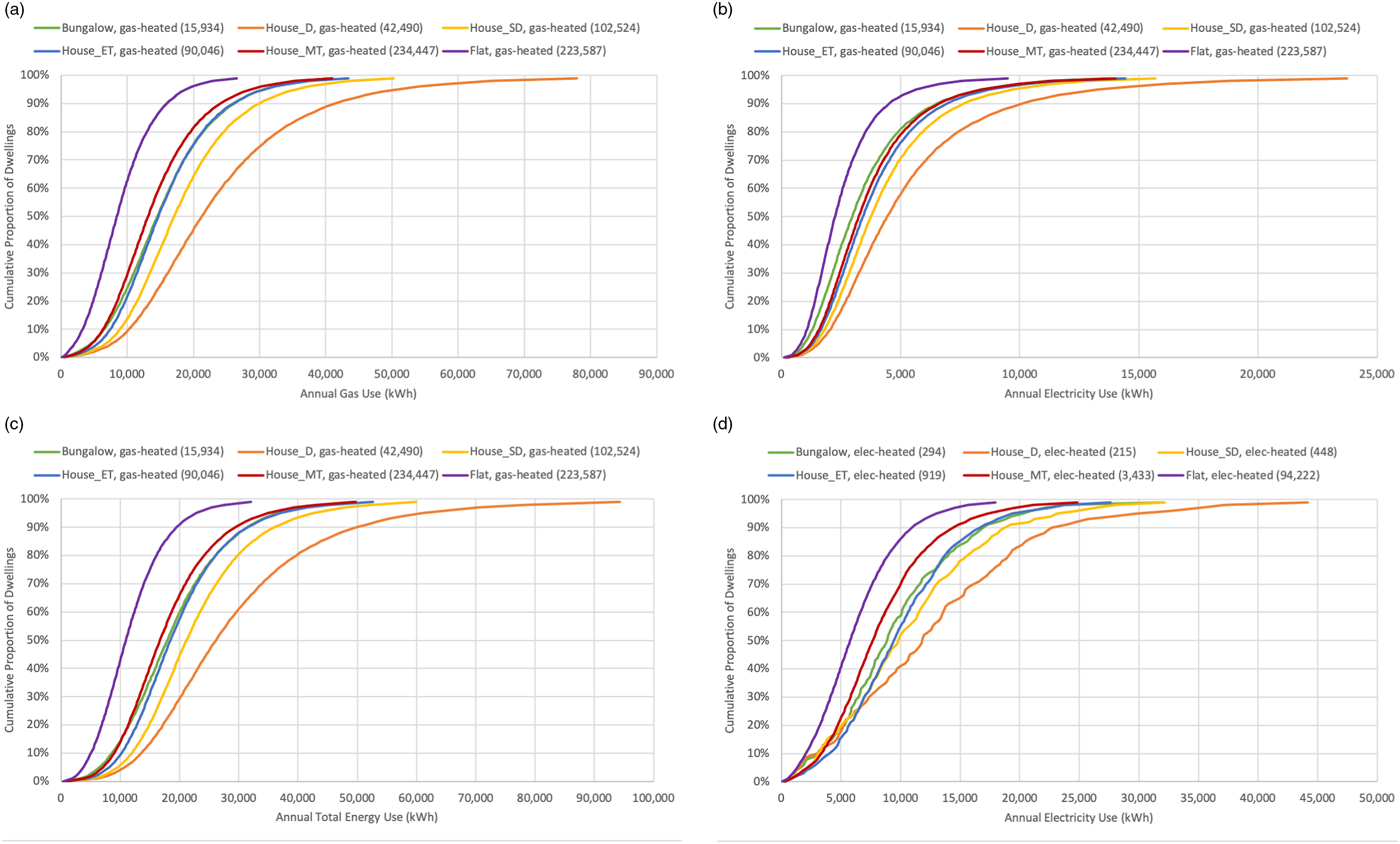

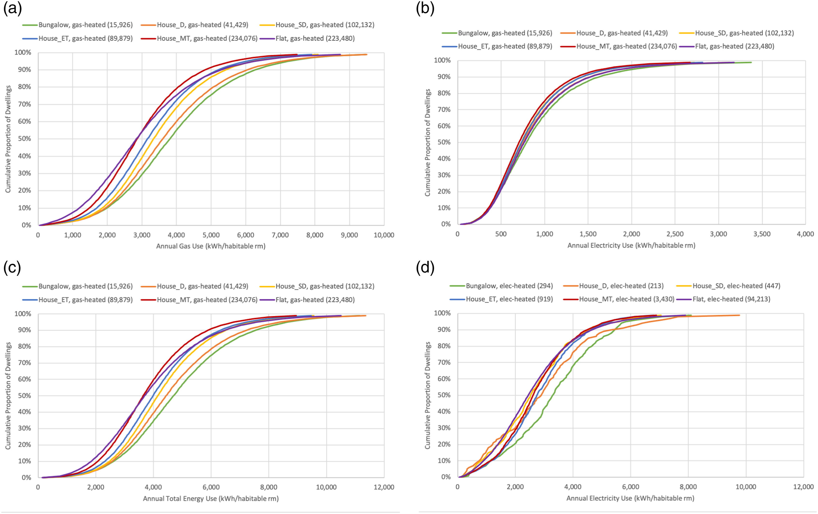
Dwelling type	Gas-heated dwellings								Electrically-heated dwellings
	Annual gas consumption				Annual electricity consumption				Annual electricity consumption
	Mean	25th	50th	75th	Mean	25th	50th	75th	Mean	25th	50th	75th
Energy normalisation process: kWh
Houses (detached)	24,380	14,823	21,226	30,113	5616	2973	4441	6,642	13,041	6,173	11,814	17,708
Houses (semi-detached)	18,648	12,528	17,072	22,866	4447	2617	3761	5,389	10,825	6309	9,795	14,406
Houses (end terrace)	16,043	10,617	14,700	19,836	4046	2374	3417	4,903	10,063	6422	9,404	12,949
Houses (mid terrace)	14,524	9,316	13,139	18,083	3857	2256	3250	4647	8498	5270	7,661	10,606
Houses (bungalow)	15,695	10,053	14,521	19,878	3603	1958	2970	4421	9751	5837	8,851	12,848
Flats	9261	5497	8,435	11,961	2653	1547	2249	3232	6295	3686	5764	8230
Energy normalisation process: kWh/room
Houses (detached)	3859	2679	3598	4734	886	524	750	1077	3012	1524	2893	3965
Houses (semi-detached)	3523	2532	3335	4309	844	518	732	1028	2686	1663	2520	3495
Houses (end terrace)	3346	2355	3162	4124	849	518	734	1035	2873	1936	2747	3646
Houses (mid terrace)	3052	2100	2862	3783	814	500	706	993	2758	1845	2608	3485
Houses (bungalow)	4007	2806	3808	4953	931	539	790	1139	3354	2264	3293	4355
Flats	3103	1913	2841	3974	899	534	763	1087	2682	1595	2447	3466

Comparison across the results reveals how the normalisation process affects the apparent relative building performance between the types, reflecting systematic differences in typical form. Considering gas-heated dwellings, for example, the kWh/m² gas use trends broadly follow compactness and electricity trends show only small differences between the types. When calculated on a per-household basis the trends broadly reflect dwelling size (from detached houses down to flats). Taking the extremes, the 25th, 50th, and 75th percentile gas intensities (kWh/m²) in flats are 74%, 84% and 91% of the equivalent values for detached houses respectively. When calculated on the basis of kWh, the same values are 37%, 40% and 40%. Taking the 25th, 50th and 75th percentiles to represent ‘good,’ ‘typical’ and ‘poor’ practice figures respectively, the poor gas (kWh) benchmark for flats is lower than the good practice benchmark for detached and semi-detached houses, and the typical practice benchmark for end- and mid-terraced houses and bungalows. In terms of statistical testing, the differences in kWh energy use in gas-heated dwellings are significant throughout: MWW, p < .01 for gas and electricity uses, when comparing houses and flats, and KW, p < .01 and the post-hoc Dunn tests show all pairs of types are significantly different for both fuels. For electrically-heated dwellings, the impact is slightly reduced, in line with the kWh/m² result: MWW, p < .01 for electricity use between houses and flats, and KW, p < .01 across the dwelling types, but the post-hoc Dunn test is insignificant for the following: bungalows and detached, end-terrace and mid-terrace houses; detached and end-terrace and semi-detached houses; and end-terrace and semi-detached houses.

Figure 6(a)–(b) illustrates the impact of the normalisation process on the relative performance across the stock. ¹⁰ The graphs show the proportion of each type that fall within the <25th, 25–50th, 50-75th and >75th percentiles of domestic energy for each normalisation type. So, for example, columns 1–3 of Figure 6(a) show gas use in detached houses; the first column shows that, 30% of detached houses have gas use within the fourth quartile (i.e. >75th-percentile) of overall domestic stock when calculated in terms of kWh/m²; while the second and third columns show that, when kWh/room and kWh are used instead, the proportion of detached houses within the fourth quartile of gas rise to 38% and 62% respectively.

Figure 6.

Distribution of (a) gas and (b) electricity use by type relative to the overall stock, for gas-heated dwellings.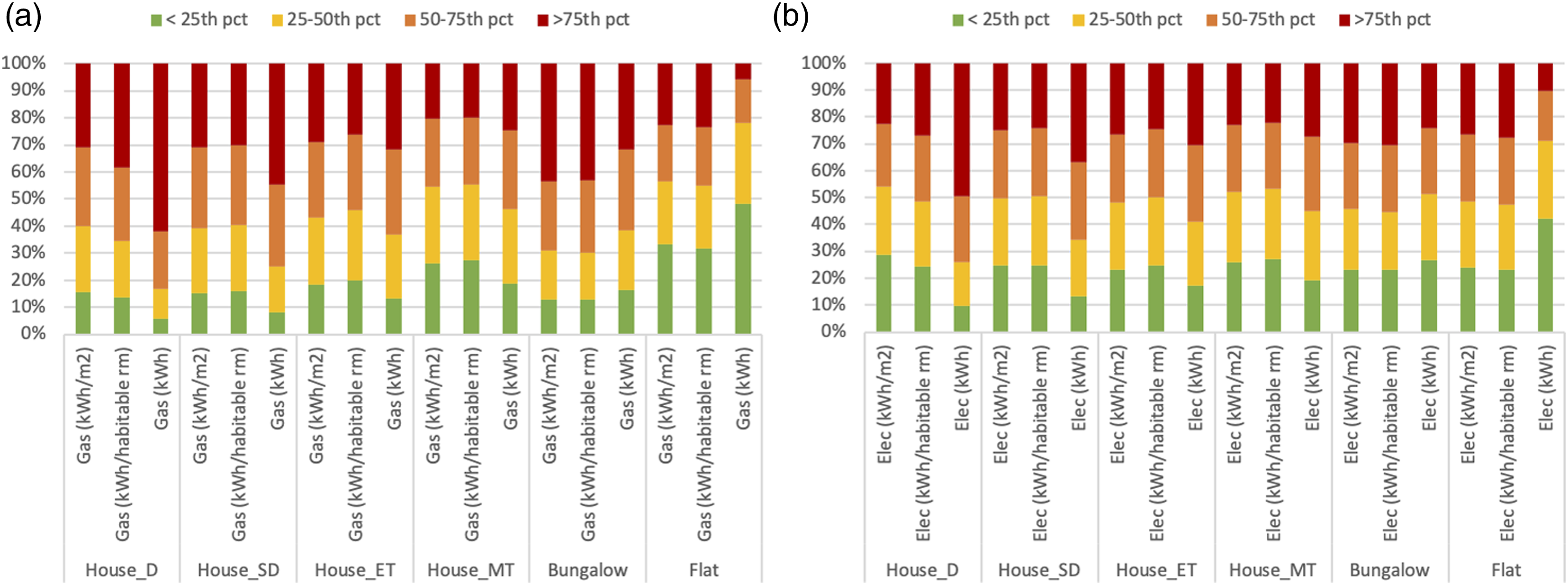

The results show how the apparent relative performance profile of each type is influenced by the measurement convention. For typically larger houses (detached and semi-detached), going from kWh/m² to kWh/dwelling results in an increased proportion categorised as very high consumers, and a reduction in the proportion identified as low consumers. The opposite is true for smaller dwellings, especially flats: The proportion with ‘good practice’ gas use (<25th percentile) falls from 16% to 6%, 15% to 8%, 19% to 13% and 26% to 19%, going from kWh/m² to kWh for detached, semi-detached, end-terrace and mid-terrace houses respectively, but rise from 13% to 16% and 33% to 48% in bungalows and flats. The equivalent values for electricity use are: 29% to 10%; 25% to 13%; 23% to 17%; 26% to 19%; 23% to 27%; 24% to 42%. Comparison of kWh/m² and kWh/room show similar results, indicating fairly consistent distributions of m²/room across dwelling types. It should be noted that habitable room count cannot be assumed to be a direct indicator of bedrooms or the number of occupants.

Energy and thermal performance

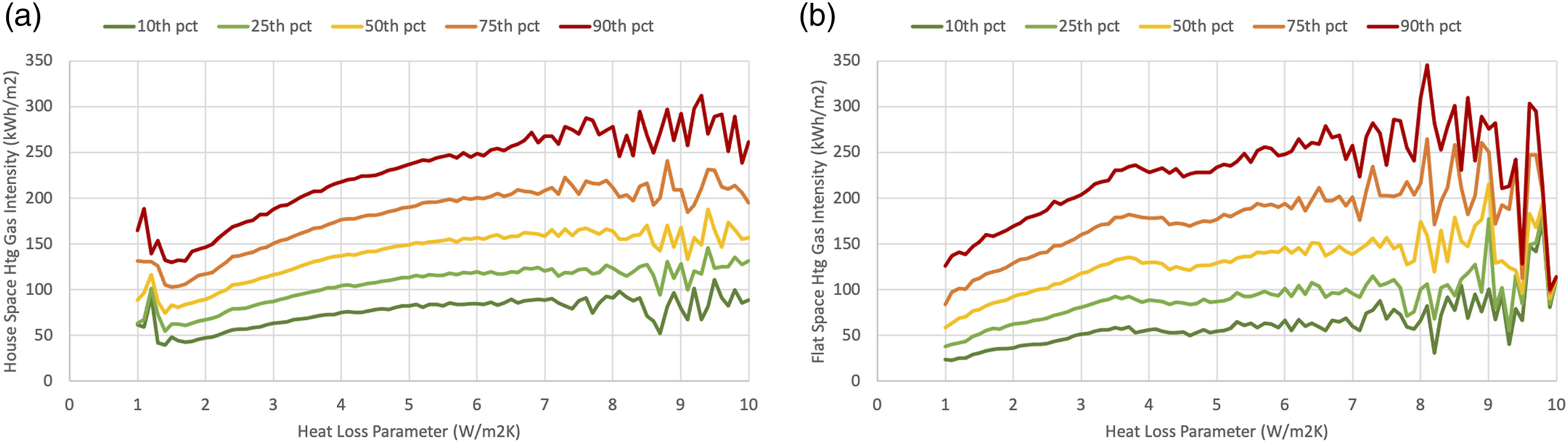
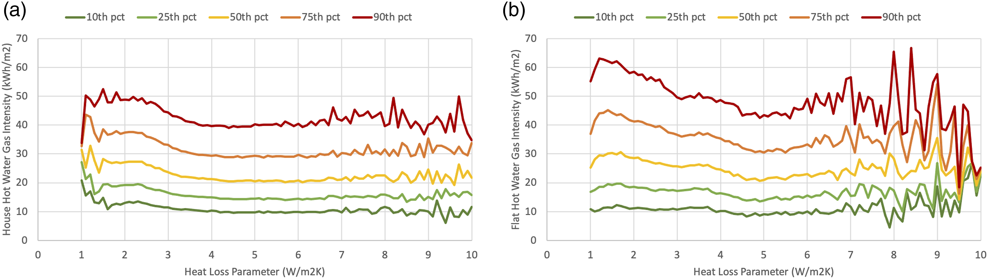
Figure 7(a)–(d) below present the overall relationship between gas use and HLP for gas-heated dwellings with boilers; ¹¹ a sample of 221,578 flats and 480,528 houses. The y-axes show the 10th to 90th percentile gas intensity figures (kWh/m²), with HLP grouped into 0.1 W/m²K bands on the x-axes. The dwelling counts are shown on the secondary y-axes. In theory, only space heating should be directly influenced by HLP. Therefore, similar results are also presented in Figure 8(a)–(b) and Figure 9(a)–(b), but split between estimated gas intensities for space and water heating respectively. Since the use split is not directly available within the existing data, space and water heating uses have been estimated for each dwelling, by multiplying its metered gas use by the ratio of estimated costs from its EPC.

Figure 7.

Relationship between HLP and gas intensity in (a) houses and (b) flats, and between HLP and electricity intensity in (c) houses and (d) flats.

Figure 8.

Relationship between HLP and estimated space heating gas intensity in (a) houses and (b) flats.

Figure 9.

Relationship between HLP and estimated hot water gas intensity in (a) houses and (b) flats.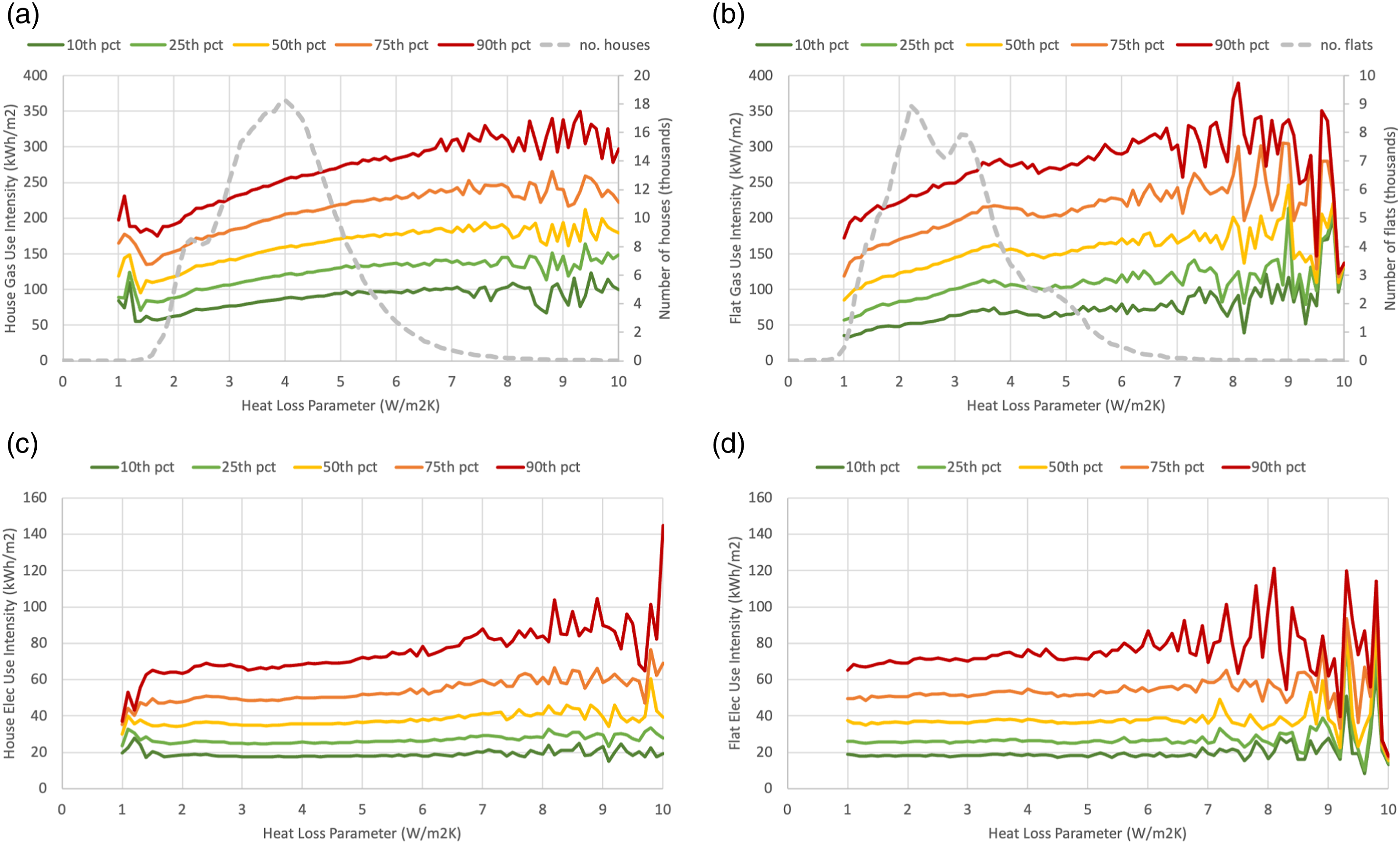

Higher HLP values correspond with worse overall thermal performance. For context, between dwellings in the sample with HLP of 1 and 10 W/m²K; typical construction age increases (49% of the former were constructed post-1990, while 90% of the latter are pre-1950); there is a higher prevalence of single glazing (fully multi-glazed dwellings drop from 95% to 78%); increased instances of solid brick walls (6% to 82%); and higher median infiltration rates and u-values (for all envelope elements). Therefore, it is reassuring that the results show clear positive correlations between gas intensity and HLP for both houses and flats. In contrast, electricity intensity shows no trend with HLP. Between houses with HLP of 2.0 and 4.6 W/m²K (corresponding with HLP interquartile range), median total gas intensity rises by 41%. For flats, the HLP interquartile range is 2.1–3.6 W/m²K, and the associated gas intensity rise is 29%. Best-fit polynomial lines, generated using SciPy optimize.curve_fit are gas EUI = (−1.964 × HLP²) + (30.740 × HLP) + 73.769 and gas EUI = (−3.007 × HLP²) + (34.168 × HLP) + 76.543 for houses and flats respectively. For both houses and flats, the results show the gas use-to-HLP gradient falling with increasing HLP (i.e. the lines curve downwards). This is in line with past studies that have shown increasing gas use with construction age (which is linked to HLP), but with non-linear correlations. ¹² These trends may be indicative of differences in the use of heat across the stock; for example, underheating in particularly under-insulated properties (or of supplementary local electric heating in gas-heated dwellings, i.e. not recorded in the EPCs). However, another factor may be the assumptions used to calculate HLP within the EPC process. For example, if all-else-being-equal, the thermal conductivity of building envelope elements in older constructions is not as poor as assumed, then the dwellings on the right-hand side of these graphs may have lower HLP values than estimated.

Considering the uses, the changes in space heating gas intensity with HLP are higher than those observed for total gas. In contrast, hot water consumption varies relatively little with HLP. Between the HLP interquartile range, space heating gas use increases by 61% and 41% for houses and flats respectively; the corresponding changes in hot water consumption are −24% and −10% for houses and flats respectively. The best-fit polynomial lines are space htg EUI = (−2.585 × HLP ² ) + (37.455 × HLP) + 32.870 for houses, and space htg EUI = (−3.384 × HLP ² ) + (39.025 × HLP) + 35.919 for flats. All-else-being-equal, the variables used to calculate HLP should not directly influence hot water energy use. However, there may be indirect factors, which explain the slight observed trends. For example, modern housing may have different typical hot water equipment than older dwellings.

Conclusion and future work

This paper describes the production of domestic energy benchmarks for the CIBSE benchmarking tool. ¹⁴ Data from a large disaggregate building stock model (3DStock) have been combined with energy consumption from meters, and heating systems data from EPCs to produce annual electricity and gas intensity benchmarks from 808,509 properties in London. The results have been presented as cumulative distribution profiles, split based on heating fuel and dwelling type (detached, semi-detached, end- and mid-terrace houses, as well as bungalows and flats). Naturally, the trends observed in the results are not unexpected; the relationships between building energy use and form and thermal envelope for example are well understood. Nonetheless, the level of detail as well as the scale of the analyses hopefully improve our understanding of domestic energy performance. The building stock is not uniform across the UK (e.g., the types of heating fuels in homes varies geographically) ⁶⁵ and this, combined with other factors like local climate, means that domestic energy use also varies. ⁶⁴ Consequently, while the sample size in this study is large (accounting for around a quarter of all domestic properties in London), application of the results to outside of the city should be treated with some caution.

Energy use in the building stock can be normalised using different denominators. While floor area is common in benchmarking and modelling^56,59 other approaches have also been used historically. ⁶⁶ Here, the results are presented in terms of annual energy use intensities (kWh/m² and kWh/room) as well as totals (kWh/household). The results show how the normalisation process influences the relative performance between the types. When calculated as intensities, heating fuel consumption trends are shown to reflect typical compactness: flats and mid-terrace houses have lower use than detached houses. However, when calculated in terms of energy, the trends reflect the systematic differences in size (e.g. flats have far lower consumption than semi-detached and etached houses). Which approach is most appropriate may depend on the circumstances and, naturally, is subjective: when considering the overall impact on national carbon emissions it may be preferable to consider the domestic stock in terms of energy or CO₂ per household, rather than normalising by dwelling size. Similarly, fuel bills are not generally standardised by size. On the other hand, when trying to understand the overall condition of the domestic stock, it may not be suitable to ‘penalise’ larger dwellings compared with smaller ones. Considering heating fuel, the results show that total energy consumption is lower in electrically-heated dwellings than gas-heated ones, reflecting differences in fuel price per unit of energy, typical occupancy demographics and building characteristics as much as the installed systems. Finally, comparison has been made between energy intensity and HLP in gas-heated dwellings. HLP is a normalised measure of a property’s overall thermal characteristics, accounting for thermal transfer through the envelope, alongside ventilation and infiltration. Reassuringly, the results show strong relationships between HLP and gas use but as the HLP increases typical energy use does not proportionally rise, that is poorly insulated homes do not use as much energy as might be expected.

It should be noted that, while the availability of large-scale disaggregate data on physical characteristics, internal systems and energy consumption has been vital to the use of stock models like 3DStock in analysing the building stock, an area where more information would be particularly beneficial is around socioeconomic factors. Household demographics, occupancy and behaviour are known to impact on domestic energy use.^22,67 Unfortunately, however, at the time of writing, the integration of such variables into models like 3DStock remains difficult as datasets tend to be published in anonymised or aggregated forms. ¹² While work is underway, using the existing data to explore performance at an aggregate level, the availability of disaggregate socioeconomic data would allow the drivers of energy use to be examined in greater detail and likely raise further issues around how the decisions around the benchmarking process impact on the apparent performance of the stock.

The work presented in this paper is part of longer-term research into the characteristics and performance of the building stock. In terms of energy use specifically, ongoing work is exploring how electricity and gas use may be driven by the detailed characteristics of buildings, as well as how those characteristics influence the relationship between modelled and actual energy consumption.

A clear understanding of the current performance of the stock is necessary for the UK to make the large-scale and long-term improvements to its homes and successfully shift towards Net Zero. This work aids the setting of targets for the transition process, but also contextualises the scale of the challenge, and feeds into scenario modelling. Major changes in the residential sector are expected in the coming years, from increased deployment of insulation improvements plus a transition towards low-carbon heating. During this transition process to new technologies, the makeup of the stock will become more heterogeneous, meaning that modelling domestic energy use may become more difficult, especially without access to sufficient and adequate empirical data. Regular updates to the domestic benchmarks on the CIBSE benchmarking tool will be beneficial through this period, to track the (hopefully significant) changes in performance that result from these measures.