
Abstract
The potential for energy, carbon dioxide equivalent (CO2e) and cost savings when using low emissivity (low-ε) transpired solar collectors (TSCs), combined with heat pumps in a range of configurations, has been investigated using computer modelling. Low-ε TSCs consist of metal solar collector plates with a spectrally sensitive surface, perforated with holes. Ambient air is drawn through the holes and heated by convection from the solar collector plate, increasing the air temperature by up to 25 K. The heated air can be used for e.g. space heating, or pre-heating water in buildings. The models developed have been used to compare the performance of low-ε TSC/heat pump heating systems in small and large buildings, at a range of locations. The model results showed savings in energy, CO2e and costs of up to 16.4% when using low-ε TSCs combined with an exhaust air heat pump compared with using the exhaust air heat pump alone.
Introduction
The UK Government has recently set a new climate change target of reaching net zero greenhouse gas (GHG) emissions by 2050. 1 Since 1990, the UK has reduced its carbon emissions by 43%, mainly as a result of carbon reduction measures in the power sector, 2 however, significantly more radical solutions and technologies will be needed to meet the new target of zero emissions by 2050. One area of focus will need to be heating, as this accounts for approximately one third of the UK’s carbon emissions and about half of its energy consumption. 3 In 2018, the European Environment Agency reported that the UK has one of the lowest shares in Europe for the use of renewable energy for heating and cooling i.e. 7%. 4 There is therefore an urgent need for alternative, flexible, low or zero carbon, renewable energy systems for use in buildings. Transpired solar collectors (TSCs) are one such technology, which can be used to facilitate the capture of solar thermal energy for heating in buildings. TSCs consist of metal plates, with a spectrally sensitive surface, which absorb solar radiation, raising their temperature. The plates are attached to a south facing (in the northern hemisphere), vertical wall of a building, such as to leave a small air gap, and sealed at the edges, to form a plenum i.e. a thin box, or cladding. The collector plate is perforated with many small holes drilled in its surface, through which ambient air is drawn, by a small fan, into the plenum. There, the air is heated by convection from the collector plate, increasing its temperature by up to 25 K. The heated air flow can then be used e.g. for space heating or for pre-heating hot water within the building.
The air temperature increase achieved depends on the environmental conditions, the solar collector plate design e.g. distribution of perforations and surface coating, and the air flow rate and face velocity of the air at its surface. 5 The coatings used by the current generation of TSCs are generally of high emissivity, which although achieving high absorption of solar radiation, are also subject to high radiation heat losses to the outside environment. However, new spectrally selective, low emissivity (low-ε) coatings have been developed, which enable the collector’s absorptivity to be maintained, while minimizing re-radiation to the environment. This results in higher collector plate surface temperatures and generates higher output air temperatures. 6
TSCs generally form part of a building’s cladding and due to their simple, unglazed construction can be installed at low additional costs relative to standard claddings, often with a marginal cost of below £50 per m2. Installations have typically achieved simple paybacks of less than 7 years.
The paper reports the results of an investigation by computer modelling of the potential of low-ε TSCs to provide solar enhanced heated air for delivery to buildings via ventilation systems. The increase in air temperatures obtained from the TSC varies with the solar radiation available i.e. from minute to minute, as well as daily and seasonally, and is only available during the day. Therefore, for an effective heating system, the TSC needs to be combined with another heating system which can be used to meet the building heat demand at other times. In this study, the heated air generated by the TSC has been used as a heat source for an air source heat pump, which is then used to meet the space heating demand profile of a building. A number of configurations for combining the TSC with the heat pump have been evaluated, and compared to the case, where the TSC is not used, to investigate its potential benefits. Traditional (high- ε) TSCs have been combined with ventilation air heating systems and evaluated previously e.g.,7,8 and the present authors have reported the use of low-ε TSCs with ventilation heating systems applied to a domestic house, 9 and a warehouse. 10 However, the current study evaluates the effect of building size, comparing small and large buildings, and investigates the effect of environmental conditions on the performance of the TSC, by applying the model at a wide range of locations.
Methodology
The evaluation of the performance of a number of configurations of TSC-heat pump building heating systems was undertaken using a modelling approach, employing Engineering Equation Solver (EES), a commercial software tool. 11 The performance of the overall heating system was simulated using a series of simultaneous equations to define the relationships between the parameters needed to describe the system. Input data for parameter values e.g. temperatures, fluid flow rates and thermal properties, were provided, and the software used to predict a number of unknown parameter values, such as the total electrical energy input to the system and the efficiency for the heat pump. In fact, to simplify the solution process, the overall heating system was divided into a number of component modules, which were then solved in sequence, in order to evaluate the overall performance of the system. The components included: (i) a TSC model; (ii) a building heat demand model; (iii) a heat pump model; (iv) a control model. The control model was needed to define the order for solving the various component models, and to switch the heat pump on and off, as required, for different input conditions. Details of the various component models are provided in the following sections.
Transpired solar collector (TSC) model
In this study, the heated air generated by the TSC device was ducted to a building, either to provide heated ventilation air directly, or to be used as a heat source for a heat pump. There was also a bypass opening in the TSC to permit ambient air to be used directly for ventilation, when solar heated air was not required. The volumetric air flow rate through the TSC was set equal to the ventilation air flow rate, which was calculated in the building heat demand model.
In earlier studies,5,6 it was found that a collector plate face velocity in the range 0.02–0.05 m/s was needed for effective operation of the TSC. By using the volumetric air flow rate through the TSC and dividing by the face velocity at the surface of the collector plate (selected to be 0.021 m/s for the current model), the required collector plate area could be calculated. In each case, the collector plate area was estimated to be substantially less than the available area of the selected building wall.
In an earlier study, 6 it was found that an air temperature increase of 20% could be obtained using a spectrally sensitive low emissivity coating for the collector plate compared with high emissivity plates, for the same absorptivity surface. 6 For each of the models in the current study, a surface absorptivity of 0.9 and an emissivity of 0.2 were assumed.
Further details of the TSC model have been provided previously. 5 A schematic of a transpired solar collector together with the energy balance at the collector plate surface is shown in Figure 1.
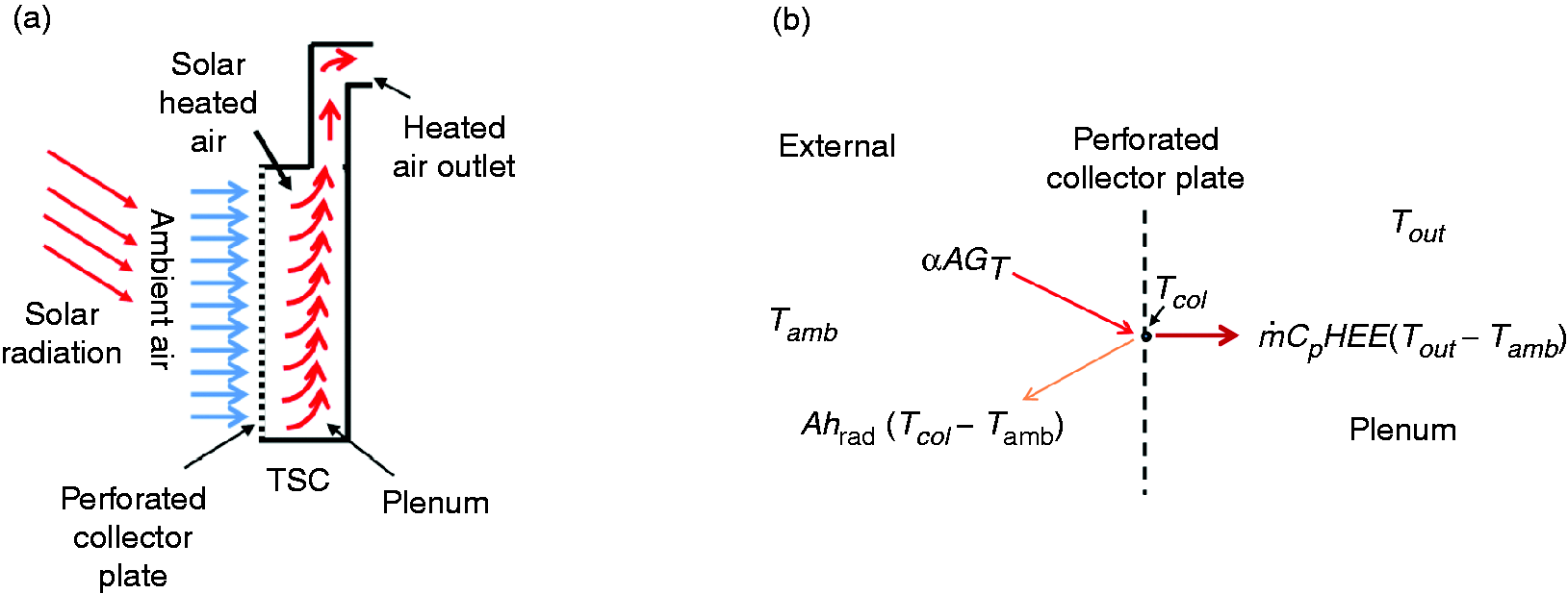
Transpired solar collector (TSC) (a) Schematic of TSC; (b) Energy balance at collector plate surface.
In Figure 1(b), α is the absorptivity of the solar collector plate surface, A is the area of the plate, GT is the solar global radiation per unit area, hrad is the linearized radiation heat transfer coefficient, which also incorporates the emissivity of the surface, and Tcol is the temperature for the solar collector surface. On the inside of the enclosure, m is the mass flow rate of the air, which enters at ambient temperature Tamb. Cp is the specific heat capacity of the air flowing through the enclosure, and Tout is the temperature of the air at the outlet. HEE is a heat exchange effectiveness coefficient which takes account of the convective heat transfer from the collector plate to the air.
12
The pressure drop through the collector plate was determined using a scaling factor used to model square pitch perforations.
13
The energy balance for the collector plate is shown in equation (1)

The heat exchange effectiveness coefficient (HEE) is defined by equation (2)
In equation (1), the main (variable) inputs needed were weather data parameters e.g. for air temperatures and solar radiation. These were obtained from a weather database,
14
for a location in the London Borough of Islington, which had been selected as a potential trial site for a prototype system. The weather data consisted of hourly values for ambient air temperature, ground temperature, sky temperature, air pressure, relative humidity, wind speed, global radiation on a south-facing vertical plane and global radiation on a horizontal plane. The overall mass air flow rate
Building heat demand model
A building model was developed to estimate the building space heating demand to be met by the heating system employed. It consisted of a simple air ventilated building, subject to heat losses through the building fabric due to the difference between the internal set temperature and the seasonal variation in outside environmental conditions, and heat losses from the exhaust ventilation air leaving the building at the internal building set temperature. To maintain the set temperature within the building, it was assumed that the required quantity of heat was added via the ventilation air supply, by raising its temperature, as appropriate. The ventilation air mass flow rate was calculated, based on the internal volume for the building and number of air changes per hour selected. The heated ventilation air supply at the appropriate temperature was generated using an air source heat pump, and supplemented by the TSC heated air. When the TSC heated air temperature reached the ventilation air temperature indicated from the building heat demand model, the heat pump could be switched off and the heated ventilation air supplied by the TSC alone.
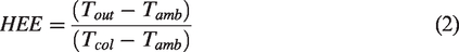
The building model assumed the building to be a rectangular box, with no internal structure, and to be heated by a single ventilation air heating system to a common temperature throughout. Two building sizes were considered, namely a small domestic building e.g. a house, and a large warehouse building. To calculate the heat demand for the building (at any particular time), the following assumptions were used:
In Table 1, the ventilation exhaust heat loss coefficient was calculated as the product of the mass flow rate of exhaust air and specific heat capacity.
Building heat demand model parameters used.
Using the assumptions in Table 1, and hourly ambient air temperatures, 15 the model was used to determine the seasonal heat demand profile for the building.
Heat pump model
The heat pump model was simulated as a single stage air source heat pump using a series of thermodynamic balance equations to link the input and output parameters and performance of each of its components. 16 Input data for the various components were specified for the model, and the equations then solved iteratively to predict selected outputs and the overall performance of the heat pump. The model comprised three main component sub-models, namely a single stage compressor, and finned tube air to refrigerant evaporator and condenser heat exchanger models. The condenser heat output capacity (which was matched to the hourly varying building heat demand) was used as input for the heat pump model, which then predicted the compressor swept volume and the electrical energy input to the compressor. It was assumed that a variable speed compressor was used, such that the capacity of the heat pump could be varied in line with the building heat demand, in order for the heat pump to take advantage of the rapidly varying input air temperature conditions provided by the solar collector output. Key inputs for the heat pump model were: (i) the condenser output capacity required; (ii) the condenser output air temperature needed; (iii) the TSC output air temperature; (iv) the volumetric flow rate for the air over the heat exchangers, which was defined by the ventilation air flow rate required for the building; (v) the condenser air on temperature, which for some configurations was ambient air, and for others was TSC heated air (vi) the evaporator air on temperature, which for some configuration options was ambient air, and for others was TSC heated air, or the exhaust air from the building (i.e. enabling it to operate as an exhaust air heat pump).
When the TSC heated air temperature was greater than the ventilation air temperature needed, while the ambient air temperature was less than the required ventilation air temperature, it was assumed that the TSC heated air could be mixed with the ambient air to produce the required air temperature, and used directly for the ventilation air supply. In this case, the heat pump would be switched off.
Control model
A key requirement for the operation of the heat pump sub-model within the overall TSC-air source heat pump-ventilation air heating system model, was a control sub-model. This was used to determine whether the heat pump was switched on or off at any particular time/set of input conditions, and to read the key parameter inputs for the heat pump model, from the building heat demand and TSC models. It was also used to provide appropriate guess values for iterative solving of the equations defining the heat pump model, in order to facilitate convergence. In addition, it controlled the sequence for execution of each of the sub-models i.e. the building heat demand model, TSC model, and heat pump model.
At any particular time (i.e. time step), the heat required to meet the building heat demand could be derived from several sources, namely: (i) directly from the TSC output air flow; (ii) after upgrading the TSC output air temperature with the heat pump; (iii) directly from the outside ambient air. It was therefore necessary to provide a control algorithm for selection of the most appropriate heat source.
A further consideration was that in some cases, very large temperature differences between the ventilation inlet air and the internal building air temperature were needed to meet the highest building heat demands, and this was undesirable with respect to the thermal comfort level within the building. Therefore, the temperature difference between the ventilation inlet air delivered Tdelivery and the building air set temperature Tset was limited to 8 K. 17 This was also accounted for in the control model. If more heat was needed to meet the building heat demand than could be achieved by the ventilation air, with this limited temperature difference (and since the ventilation air flow rate was fixed), it was assumed that the difference in heat capacity was made up by an electric heater (with 100% efficiency) located within the building. The cost and carbon emissions associated with this additional electricity input needed to meet the building heat demand were also calculated, and added to the totals for energy, carbon and cost inputs for the heating system.
Ventilation heating system configurations modelled
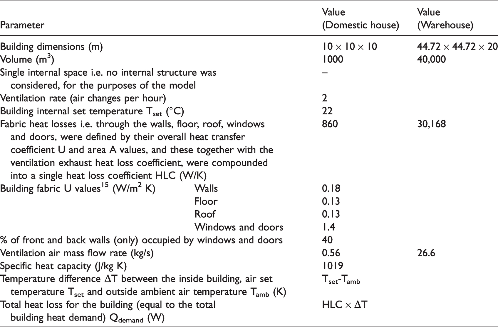
In Figure 2, TSC is the transpired solar collector and HP is an air source heat pump. The four heating system configurations shown were each modelled with: (i) the TSC in operation; and (ii) in bypass mode, where ambient air only was provided.
Ventilation air heating system configurations modelled. (a) Electric heating of building only; (b) Heat pump with ambient or TSC air onto condenser, ambient air onto evaporator, and electric heater top-up; (c) Heat pump with ambient or TSC air onto condenser, exhaust air onto evaporator, and electric heater top-up; (d) Heat pump with ambient air onto condenser, ambient or TSC air onto evaporator, and electric heater top-up.
For the three configurations using heat pumps shown in Figure 2, where either the ambient air or TSC heated air temperatures reached or exceeded the building heat demand ventilation air temperature required, the heat pump was assumed to be switched off within the model.
Results
The results from the modelling work are presented in the following sections.
TSC model
TSC heated air temperatures
Figure 3 shows the results for seasonal variation in TSC heated air output temperatures in comparison with ambient temperatures, predicted by the model.
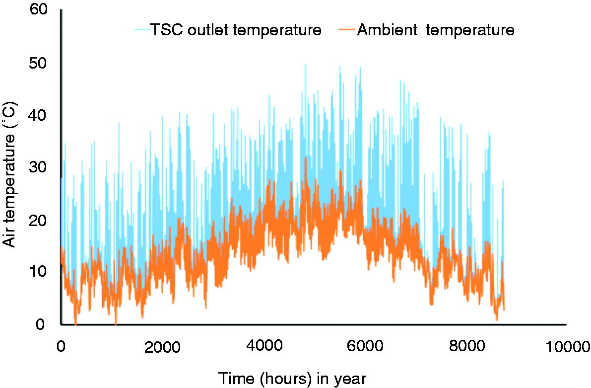
Annual temperature profile for TSC outlet air for London location.
It is seen that there was a significant increase in temperature for the TSC outlet air compared to ambient air, of up to 25 K, however, the TSC outlet air temperature increase varied significantly (in the range 0–25 K) from hour to hour. It should be noted that the air temperature profiles both with and without the TSC were effectively identical for the small (domestic) building and large (warehouse) building.
Rise in air temperatures in TSC
A comparison of the rise in air temperatures in the TSC for the four different locations considered, namely London, New York, Stockholm and Southwest Florida is shown in Figure 4.
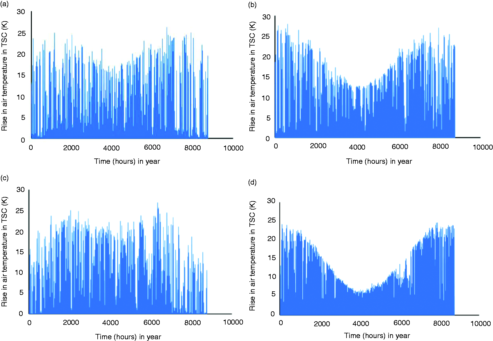
Temperature rise in TSC at four locations. (a) London; (b) New York; (c) Stockholm; (d) Southwest Florida.
The profiles for temperature rise in the TSC were distinctly different for the four different locations. In most cases the maximum temperature rise in the TSC was of the order of 25 K, although some slightly higher temperature rises of up to 28 K were seen for the New York location, in winter. For the London location, temperature rises were of the order of 20–25 K for most of the year, but were reduced to approximately 16–18 K for about 1000 h in the middle of summer. The temperature rise profile in the TSC for the Stockholm location also showed increases of 20–25 K for most of the year, but with no reduction in summer. However, the Stockholm location showed reduced temperature rises of 12–15 K for approximately 1000 h in the middle of winter. In contrast, for the two USA locations i.e. New York and Southwest Florida, the temperature rise in the TSC was highest in winter, but decreased steadily to a minimum in the middle of summer. The minimum temperature rise in the TSC for the New York location was approximately 14 K, while for the Southwest Florida location it was approximately 7 K.
Building heat demand model
Comparison of small (domestic) building and large warehouse building
The annual building heat demand profile for the small and large buildings considered, both for the London location, are presented in Figure 5. The figures show the daily variation in heat demand for each building in kWh, over a year. The heat demand values predicted by the model are based on the ventilation air mass flow rate, the set temperature selected for the building, and weather data, and depend particularly on the outside, ambient air temperatures.
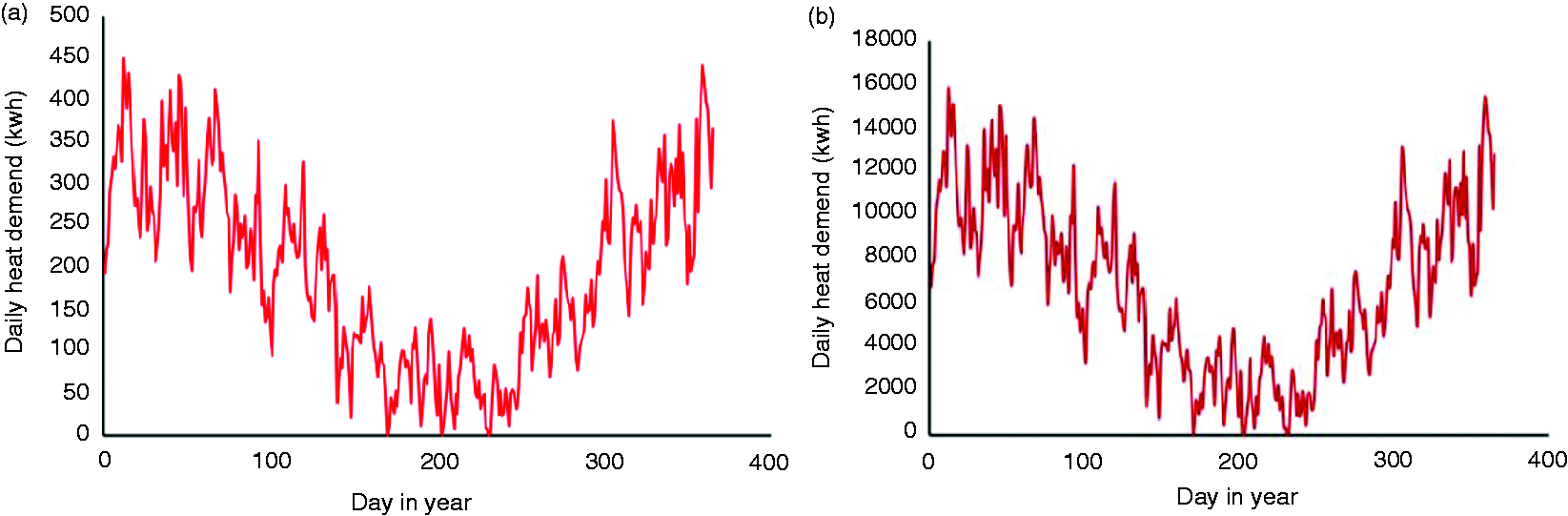
Seasonal variation in building heat. (a) Small domestic building (house); (b) Large building (warehouse).
In Figure 5, the daily heat demand, follows a sinusoidal trend over the year, with the highest heat demand, of approximately 400 kWh per day for the small domestic building and 16,000 kWh per day for the large warehouse building occurring during the winter months. In each case, the heat demand then decreases to a minimum level of 0 kWh at times during the summer months, although varying by up to 100 KWh for the small building and 4000 kWh for the large building from day to day, throughout the year.
The building heat demand models were used to predict the temperatures needed for the ventilation air supplied to the building, in order to replace all of the heat losses from the building i.e. to match the heat demand value, on an hourly basis, throughout the year.
Comparison of building heat demand profile at four locations
A comparison of the building heat demand profiles for the large warehouse building at the four locations considered, namely London, New York, Stockholm and Southwest Florida are shown in Figure 6.
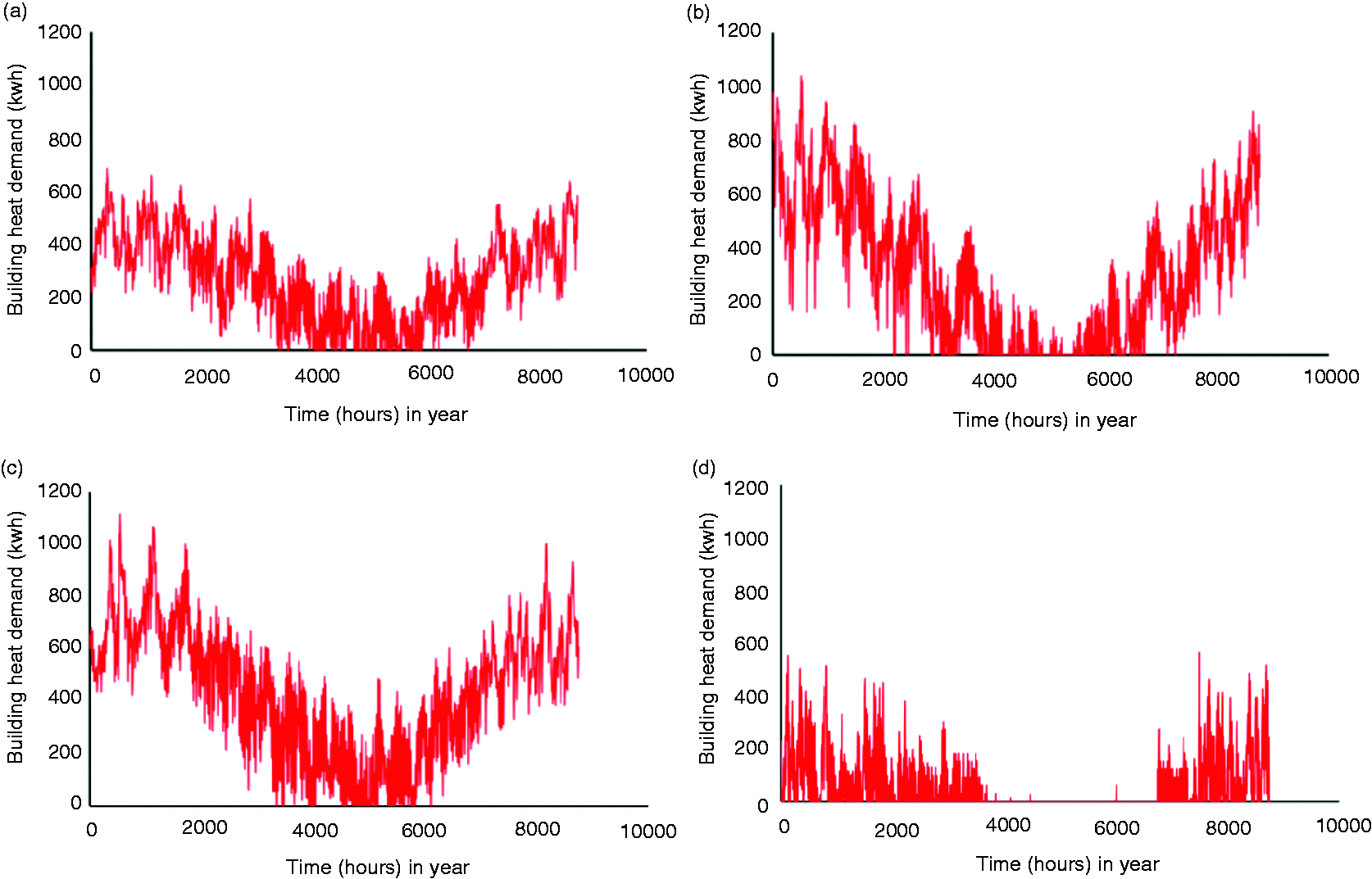
Comparison of building heat demand profiles for warehouse building for four different locations. (a) London; (b) New York; (c) Stockholm; (d) Southwest Florida.
Comparing the building heat demand profiles for the four locations, on an hourly basis, for the large (warehouse) building, using the same axis scaling for each graph, showed some distinct differences. For the London location, the hourly building heat demand varied sinusoidally from a maximum of 600 kWh in winter to a minimum of 0 kWh, at times, in summer, although with an average heat demand of approximately 100 kWh for 2200 h i.e. three months, in summer. In contrast, for the New York location, a larger amplitude sinusoidal variation was seen, with a maximum building heat demand of 1000 kWh in winter decreasing to a minimum of 0 kWh in summer, with an average heat demand of 0 kWh for 1500 h i.e. 2 months, in summer. For the Stockholm location, a building heat demand profile combining parts of both the London and New York profiles is seen, with a maximum of 1000 kWh in winter, a minimum of 0 kWh in summer, but with an average heat demand of approximately 150 kWh for 2200 h i.e. 3 months, in summer. The Southwest Florida location shows a much lower heat demand than for the other locations, with a maximum of 500 kWh in winter, but zero heat demand for 3000 h i.e. 4 months, in summer.
Results for heat pump model and analysis
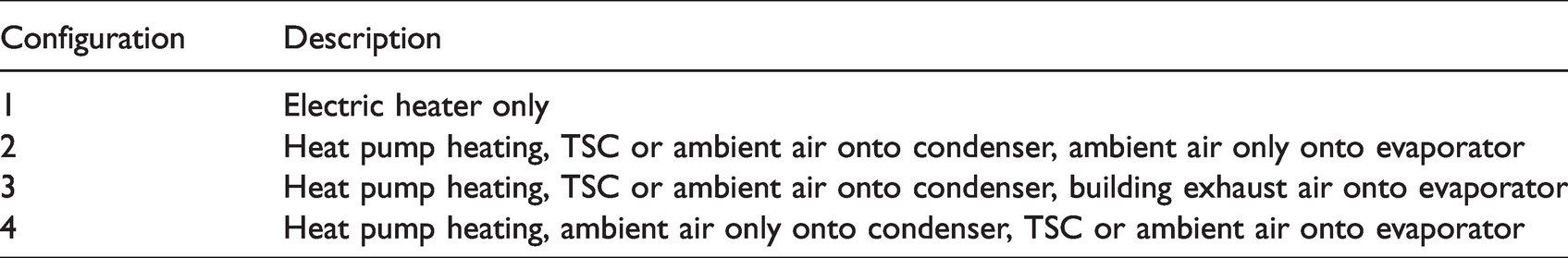
A summary of the heating system configurations considered is shown in Table 2.
Air ventilation heating system configurations.
The outputs from both the TSC model and building heat demand model, together with hourly ambient air temperatures, derived from the weather data, were used as inputs for the heat pump model. The model was then used to determine the total electrical energy needed to supply both the heat pump compressor and heat exchanger fans, together with any additional top up by the electric heater if required, in order to meet the required heat output capacity and ventilation air delivery temperature.
The overall electrical energy used by the ventilation air heating system was then used to calculate the corresponding CO2e emissions and estimated cost for the electricity, for each of the configurations considered both with and without the TSC heated air in operation. Assumptions used in calculating the carbon dioxide equivalent (CO2e) emissions and costs were: (i) an electricity carbon factor of 0.2555 kg CO2e per kWh of electricity used 18 ; and (ii) a cost for electricity of £0.155 per kWh of electricity. 19
Comparison of performance of four heating system configurations for small domestic building
A comparison of the results for electrical energy input, CO2e emissions and costs for the four heating system configurations for the small, domestic building, at the London location, are shown in Figure 7.
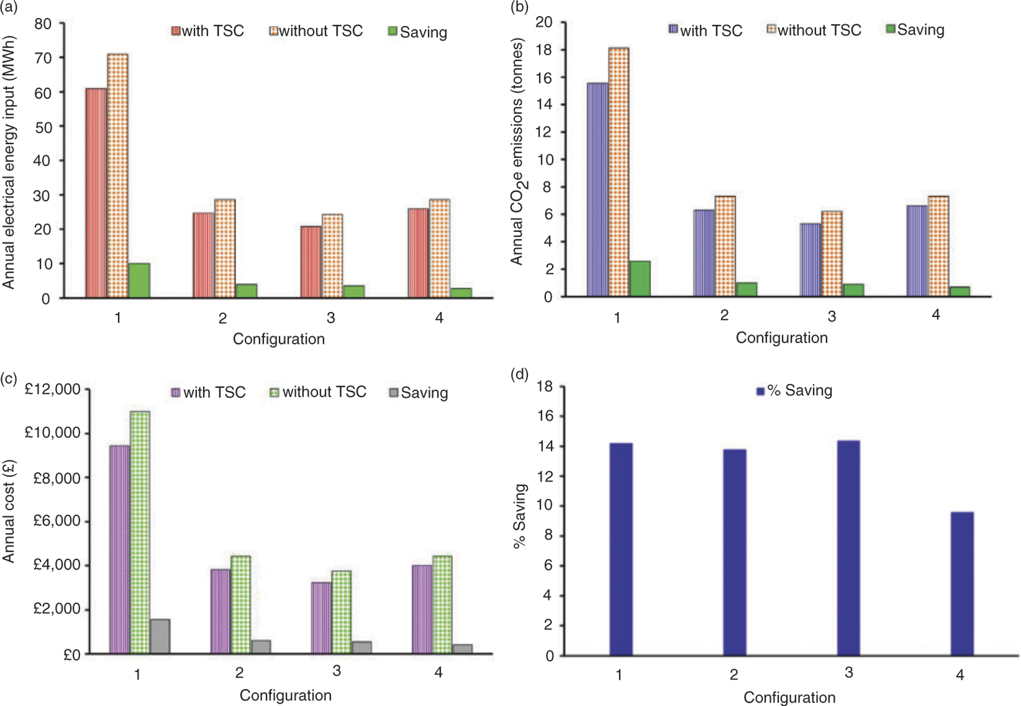
Energy, carbon emissions and cost savings with TSC for four heating system configurations for small, domestic building (house), located in London, UK. (a) Annual electrical energy input; (b) Annual CO2e emissions; (c) Annual costs; (d) % Saving.
It is seen in Figure 7 that the heating system configuration with the lowest electrical energy use, CO2e emissions and costs was configuration 3 i.e. the exhaust air heat pump. This system also demonstrated a further benefit of an additional energy, emissions and cost saving of 14.4% from using the TSC device. The electrical heating only system (configuration 1) showed similar % savings when using the TSC, however, its overall energy use was much greater i.e. of the order of three times that of the heat pump based heating systems (configurations 2, 3 and 4). Considering the other two heating system configurations, for configuration 2, the standard heat pump system with TSC heated air directed onto the condenser, the energy input was a little higher than for the exhaust air heat pump (configuration 3), and the % saving with the TSC marginally lower i.e. 13.8%. However, for configuration 4, the standard heat pump with TSC heated air directed onto the evaporator, while the energy input was similar to configuration 2, the % saving with the TSC was significantly lower i.e. 9.6%.
Comparison of performance of four heating system configurations for large warehouse building at four locations
The four heating system configurations at the four locations considered i.e. London, New York, Stockholm and Southwest Florida were compared, for the large warehouse building. The results for annual electrical energy input for each heating system configuration at the four locations are shown in Figure 8.
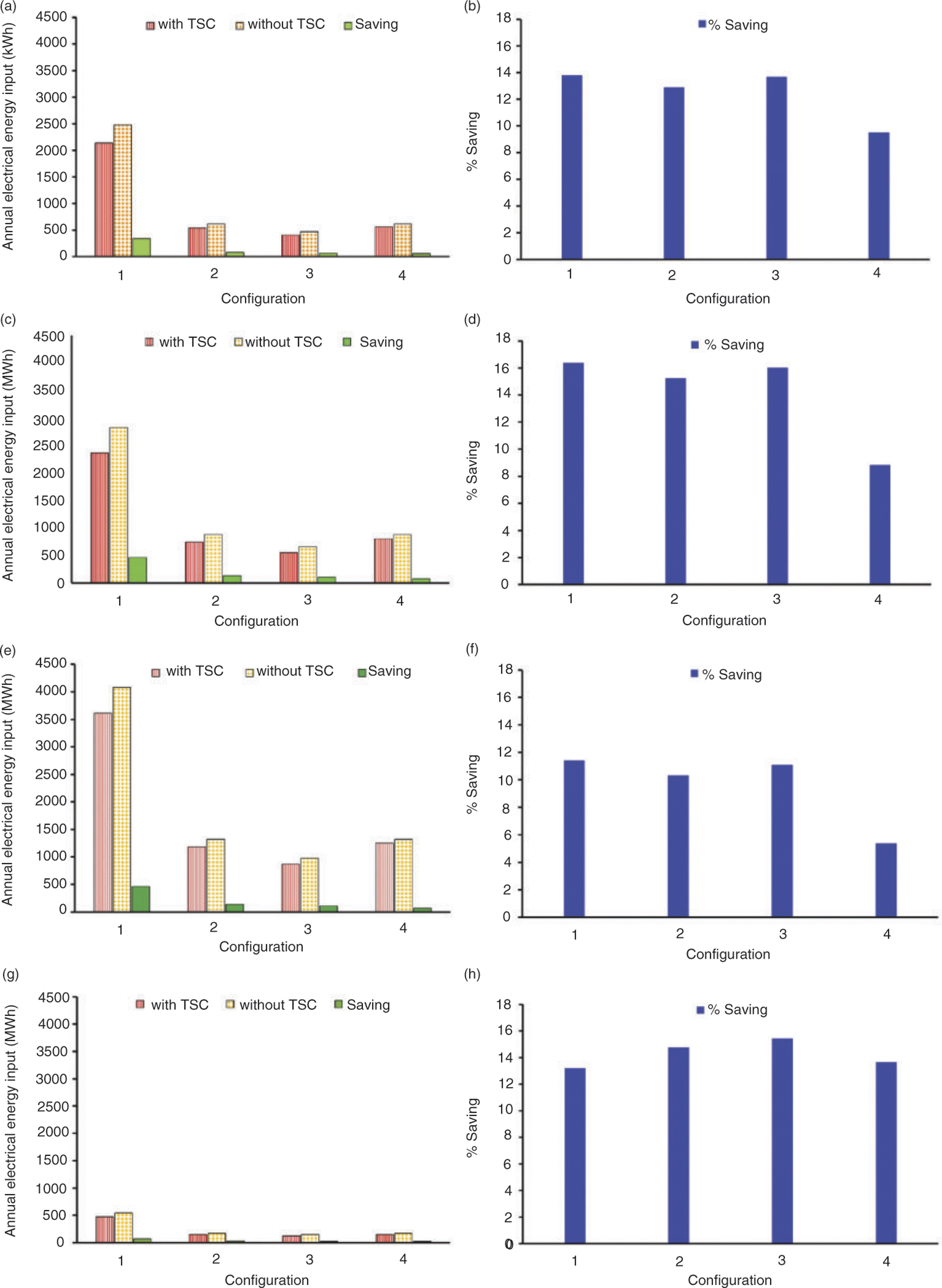
Annual electrical energy inputs and % Saving for four heating system configurations for warehouse building at four locations. (a) Annual electrical energy – London; (b) % Saving – London; (c) Annual electrical energy – New York; (d) % Saving – New York; (e) Annual electrical energy – Stockholm; (f) % Saving – Stockholm; (g) Annual electrical energy – Southwest Florida; (h) % Saving – Southwest Florida.
It is seen in Figure 8, that the pattern of annual electrical energy input values for the four heating system configurations was the same for all four locations. In each case, the highest electrical energy input was for the electric heating only system (configuration 1), however, significantly lower but similar electrical energy inputs were calculated for the two standard heat pump systems (configurations 2 and 4). The lowest electrical energy input for all locations was the exhaust air heat pump (configuration 3).
The greatest % saving with the TSC was also for configuration 3, at each location, although a similar high % saving was achieved for the electrical heating only system i.e. configuration 1, for the first three locations (Figure 8b, d and f). A marginally lower % saving with the TSC for configuration 1 compared to configuration 3 was observed for the Southwest Florida location (Figure 8h).
The highest % saving with the TSC i.e. 16.1% was achieved for configuration 3 for the New York location. The % saving with the TSC was also high i.e. 15.4% for configuration 3 for the Southwest Florida location, although the annual electrical energy inputs for this location were much lower than for the other three locations. For the Stockholm location (Figure 8e and f), the % saving with the TSC for configuration 3 was a little lower i.e. 11.1%.
Due to the relatively high room temperature setting selected for the building model i.e. 22 °C, it is seen in Figure 6a and c, there is some heat demand throughout the year for the London and Stockholm locations. In practice, space heating might not be used during the summer months, and the building temperature allowed to fluctuate with the ambient temperature at this time. Therefore, these models have been re-run with the assumption of a heating season of 7 months only for the London and Stockholm locations, with no heat input for 5 months of the year. Under these conditions, although the annual heat demand was reduced, the relative performance of the different heating system configurations remained the same. However, there was a reduction in the % saving when using the TSC of approximately 2%, in each case, highlighting the potential benefits of employing the TSC during the summer months. Therefore, although there are still substantial benefits from employing the TSC for a 7 month heating season only, there is also a case for utilising the heat output of the TSC for e.g. domestic water heating or thermal storage during the summer, to take advantage of the solar gain over this period.
Although only the annual electrical energy inputs for each heating system are reported here, since the annual CO2e emissions and costs were calculated from the annual electrical energy input values for each configuration, the % savings with the TSC were the same, in each case.
Discussion
TSC model
TSC heated air temperatures
The TSC outlet seasonal temperature profile shown in Figure 3 follows a similar pattern to that for ambient temperatures, although with increased temperatures of between 0 and 25 K. A similar level of increase in TSC outlet temperatures above ambient is seen throughout the year. There are, however, significant differences in TSC output temperatures from hour to hour, reflecting the variation in solar radiation availability. In fact, the performance of a TSC can be reduced in buildings with an early morning or late evening dominated heating demand, since a large proportion of the heating demand will be at a time when there is little or no solar radiation available. 5 In this case, the performance i.e. % saving, with the TSC could be improved by incorporating thermal storage, to store heat generated in excess of demand during the middle of the day, and then using it in the early morning/late evening or at night. It has been previously observed, 20 that factors affecting the TSC absorber plate thermal efficiency include irradiance, air flow rate through the TSC, outside air temperature, wind speed and direction.
Rise in air temperatures in TSC
The rise in air temperatures in the TSC for the four locations considered (Figure 4) show some distinct differences in variations in temperature rise through the year. In each case, the maximum rise was of the order of 20–25 K, which was in line with the maximum expected for the TSC based on previous studies. 6 In general, the highest temperature rises occurred in the winter months, with reduced temperature rises during the summer months. This probably reflects the fact that it is easier to generate a temperature difference between the TSC solar collector plate and the ambient air in winter. It is apparent, however, that there is a concentration of the number of hours at which a temperature rise was observed in summer, so the overall solar collection is likely to be greater at this time. One exception to the general trend is for the Stockholm location (Figure 4c), which showed slightly lower temperature rises during the winter months. This may be due to the more northerly latitude of Stockholm compared to the other locations, whereby the global solar radiation is marginally reduced in winter.
Building heat demand model
Comparison of small and large buildings
The seasonal building heat demand profiles in Figure 5a and b show a clear annual trend i.e. higher heat demand in winter and much reduced demand during the summer months, although with significant day to day variation. The building heat demand effectively mirrors the seasonal variation in ambient temperatures, and follows a typical seasonal pattern for heat demand in buildings. 21 The building heat demand profiles were effectively identical for the small domestic building and large warehouse building, at the London location, although with proportionally higher heat demand for the larger building.
The building heat demand model was used to calculate the hourly variation in ventilation air temperatures to be supplied to the building in order to meet demand, and these were used as input for the heat pump model.
Comparison of building heat demand profiles at four locations
The building heat demand profiles for the large warehouse building at the four locations considered are shown in Figure 6, and demonstrate some significant differences. The greatest seasonal variation in building heat demand was for the New York location (Figure 6b). A slightly lower seasonal variation was found for the Stockholm location, although with increased heating demand in summer compared to the New York location. For London, there was a much smaller seasonal variation in building heat demand than for the New York and Stockholm locations. The lowest overall heat demand was for the Southwest Florida location, with no heat requirement at all for 4 months in summer. The building heat demand profiles observed reflect the different environmental (weather) conditions for the four locations, particularly seasonal variation in ambient air temperatures and solar radiation.
Heat pump model and analysis
Comparison of performance of four heating systems for small building
The annual electrical energy input, CO2e emissions and costs for the four heating system configurations both with and without the TSC included, for the small building, are shown in Figure 7. The electric only heating system (configuration 1) indicated the highest values for each parameter (i.e. electricity input, CO2e emissions and costs) and therefore was the least useful and least economic of the four heating systems considered. However, configuration 1 demonstrated high potential savings of 14.2% when the TSC was used. The three heat pump based heating systems all required much lower electrical energy inputs which resulted in much lower CO2e emissions and costs i.e. approximately one-third that of the electric only heating system. The best performing system with the lowest electrical energy input requirement (and lowest CO2e emissions and costs) was the exhaust air heat pump (configuration 3). Configuration 3 also demonstrated the highest % saving of 14.4% when the TSC was used. For the other two heating systems i.e. configurations 2 and 4, reduced savings when using the TSC of 13.8% and 9.6% respectively were determined by the model. In the case of configuration 2, TSC heated air was directed onto the condenser and ambient air onto the evaporator. However, for configuration 4, TSC heated air was directed onto the evaporator and ambient air onto the condenser. Therefore, the most effective way of utilising the TSC heated air with a heat pump based air ventilation heating system is by directing it onto the condenser.
The model was also used to evaluate the performance of the large, warehouse building at the London location. Similar patterns of energy use, CO2e emissions and costs, were found, although with proportionally higher values for each parameter for the larger building. The % saving when using the TSC was also similar for the warehouse building, although marginally lower i.e. 13.7% for configuration 3, compared to 14.4% for the small building.
Comparison of four heating system configurations at four locations
A comparison of the performance of the four heating system configurations for the four locations considered, namely London, New York, Stockholm and Southwest Florida are shown in Figure 8. The relative performance of the heating systems was the same for each location i.e. with configuration 3 (the exhaust air heat pump) performing best, followed by the other two heat pump based systems (configurations 2 and 4), with the electric only heating system (configuration 1) being the most energy intensive and having the highest emissions and costs. In terms of benefit i.e. % saving, from using the TSC, the exhaust air heat pump (configuration 3) again performed best, at each location. The highest % (annual) saving when using the TSC was 16.1% for the New York location. This compared with a % saving for the Southwest Florida location of 15.4%, for London of 14.4% and Stockholm of 11.1%. It is considered likely that the % annual savings with the TSC determined for the different locations reflects the seasonal availability of solar radiation at these locations, and this is largely dependent on their latitudes. Considering three of the locations only i.e. New York, London and Stockholm, in terms of their latitudes; New York has the lowest latitude of 41°N, London has a latitude of 51°N, and Stockholm a latitude of 59°N, and this corresponds to the order of % savings with the TSC at these locations. An exception to this trend is the Southwest Florida location which has the lowest latitude of all i.e. 26°N, so would be expected to obtain the greatest benefit from the TSC i.e. highest % saving. However, the overall building heat demand was very low for Southwest Florida compared to the other three locations, and for 4 months in the summer (when solar radiation availability was greatest) no heat was required. Consequently, there was less opportunity for the TSC to enhance the four heating systems, so may explain why the % saving was a little lower than would be expected in relation to its latitude.
Conclusions
This study has investigated the effects of using a low-ε TSC device to generate heated air, when incorporated into a range of configurations of ventilation air space heating systems for buildings. The configurations evaluated included an electric heating only system and three heat pump based heating systems, both with and without the TSC included. Using models, the effects of building size and environmental conditions, at a range of locations have been investigated. The electrical energy input, CO2e emissions and operating costs were determined for each configuration.
In each case, the electric heating only system required very high energy input, resulting in high CO2e emissions and costs i.e. by more than three times that for any of the heat pump based systems, for the small, domestic building (Figure 7), and by more than four times for the large, warehouse building, for the London location (Figure 8a).
For both the small and large buildings and for all locations, the best performing system i.e. that with the lowest electrical energy input, CO2e emissions and costs was configuration 3, the exhaust air heat pump. Significant additional savings were achieved for all heating system configurations i.e. both the electric only and heat pump based systems, for both building sizes and at all locations, when the TSC was used, with values (for configuration 3) ranging from 11.1% to 16.4%. In each case, the greatest % saving was for configuration 3 i.e. the exhaust air heat pump, with savings of 14.4% and 13.7% for the small and large buildings respectively, for the London location. However, the greatest saving when using the TSC was 16.4% for configuration 3, for the large warehouse, at the New York location, although very significant savings were achieved at all of the locations considered. However, it was concluded that, in general, the % saving with the TSC increased with decreasing latitude, with increasing % savings in the order Stockholm, London and New York. The exception to this was the Southwest Florida location which had the lowest latitude of all, but indicated the second highest % saving. It was concluded that this location was anomalous due to having a very low annual heat requirement, and having zero building heat demand for 4 months during the summer (and the heating system was switched off), when solar radiation availability was at its maximum.
The results for the three heat pump based systems i.e. configurations 2, 3 and 4, for both the small and large buildings, and for all locations, were compared. It was seen that when the TSC heated air was directed onto the condenser i.e. configurations 2 and 3, significantly higher % savings were achieved than for configuration 4, when the TSC heated air was directed onto the evaporator. Therefore, in order to maximise the benefit obtained from the TSC for a heat pump based air ventilation heating system, the TSC heated air should be directed onto the condenser.
Other potential benefits of using TSCs are that they can act as cladding for buildings, providing extra insulation, and reducing fabric heat losses. In future work, it is planned to investigate the use of low-ε TSCs in other building heating system configurations. Also, the use of low-ε TSCs with other building types and for pre-heating of hot water for buildings, and for combining with storage systems to provide better utilisation of the TSC generated heat will be investigated.
Overall, it is concluded that low-ε TSCs offer significant benefits in providing low cost, low carbon heating for buildings.
Footnotes
Declaration of conflicting interests
The author(s) declared no potential conflicts of interest with respect to the research, authorship, and/or publication of this article.
Funding
The author(s) disclosed receipt of the following financial support for the research, authorship, and/or publication of this article: This research was undertaken as part of the ‘Steel Zero and its Low Carbon Heating Applications’ project, which is funded by HM Government Department of Business, Energy and Industrial Strategy (BEIS) Low Carbon Heating Technology Innovation Fund.