An update of the UK’s design summer years: Probabilistic design summer years for enhanced overheating risk analysis in building design

Abstract

Overheating is increasingly becoming a key issue for building design across the world. In the UK, better building fabric performance and warmer weather can increase the risk of overheating events in badly designed buildings. The impacts of these overheating events could be reduced by adapting building designs at an early design stage using building thermal models using appropriate weather data such as a design summer year. In this work, a method to determine probabilistic design summer years will be presented. These years take into account the return periods of actual events, are presented within a probabilistic framework and therefore include a description of the severity of the year at each location.

Practical application: Design summer years are designed to be used to optimise building performance in terms of thermal comfort at design stage. This paper demonstrates a method to create probabilistic design summer years which contain a range of overheating events which can be used to inform designers of the overheating risk to occupants. The proposed method is then used to generate new near extreme weather files for the UK.

Introduction

Building thermal modelling is regularly used as part of the building regulation compliance assessment and as a way of influencing design decisions. In the UK, this includes the modelling of energy use and carbon emissions to meet targets as set out within part L. ¹ Such modelling usually makes use of a weather file containing an hourly time series of the important weather variables (such as temperature, relative humidity, solar radiation and wind speed) at a location near to where the building will be sited. In the UK, modelling is often completed with two files. One, termed the test reference year (TRY) represents a typical year, the other, the design summer year (DSY), represents a year with a warmer than typical summer.

The concept of a DSY was established in 2002 ² with the purpose that building designers could test their designs in near extreme conditions to evaluate the risk of overheating using dynamic thermal models. The number of locaions was increased, from the initial 3, to 14, in 2006. ³

The method of selecting the DSY is relatively straight forward. The mean temperature over the period April to September inclusive for each year in the observation series is calculated and the chosen year is the third hottest. However, over the years, it has become apparent that this original DSY can provide less overheating in terms of the hours over a 25℃ and 28℃ than the TRY for the same location, while for other locations, such as Leeds, the DSY can be much more severe than would be expected for the latitude. Jentsch et al. ⁴ formalised the issues with the CIBSE method and can be summarised as:

The severity of the DSY varies across all locations – the severity problem.

The tails of the temperatures distribution for the TRY can be more extreme than that of the DSY – the temperature problem.

A number of sites can produce more overheating using the TRY than the DSY for a number of building types – the overheating problem.

This has consequences for building design as it brings into question the whole idea of the DSY representing an atypically warm summer. The causes for the failure though are numerous and go beyond revisiting the data availability as the structural deficiencies of the simplistic selection method would not be addressed. ⁵ Overheating in buildings is not associated with slightly above average temperatures over an extended period of time as per the definition of the DSY. Overheating is usually defined as a period where the internal temperature is above what is considered by an occupant to be comfortable. As such, it is more typical to experience overheating with shorter periods of weather which are extreme compared to the typical conditions.^6,7 Selecting the year with the third warmest mean temperature over a six month period has no guarantee of selecting such a period of extreme weather. ⁴ The original DSY, although simple to define, has no basis to produce a year with any overheating events.

Recently, probabilistic design summer years (PDSYs) were developed for the London area ⁸ in an effort to replace the London DSY with a set of years which better describe overheating events, their relative severity and their expected frequency. Here, this methodology will be extended to create PDSYs which are consistent across all 14 CIBSE locations. ³ A brief overview of the potential overheating criteria will be described as well as statistical methods used to characterise a range of hot weather events. The buildings’ response to the external temperature depends on the form of the building as well as how it is used. As such, it is not possible to define a control building which can represent all possible buildings so a simplification must be made. In this research, a conceptual building will be used as defined in TM49. ⁸ The building is free running and the operative temperature is equal to the external air temperature at all times. This building is equivalent to a building with a high ventilation rate where all external gains are removed and the external temperature is equal to the internal temperature. While this conceptual building is a clear simplification as it does not include the effects of thermal mass or solar gain through windows, it is easy to implement as external temperatures can be considered as a proxy for the internal temperatures. Finally, probabilistic design weather years for all CIBSE locations will be presented.

Updated weather data for new weather years

Using a more recent baseline to develop new weather years has the advantage that any changes in the observed climate are taken into account and buildings can therefore be designed to take into account such changes. In the previous approach, 21 years of data were considered sufficient to describe the baseline climate. ³ However, climatologists typically use longer periods of observations to compare current climatological trends to that of the past or what is considered ‘normal’. A normal typically consists of a 30-year period, as it is long enough to filter out any inter-annual variation, but also short enough to be able to show any longer climatic trends. Thirty years has been used within the climate change projections UKCP09 to investigate as the underlying climate trends ⁹ and was used to evaluate the effects of climate change. ¹⁰

In this work, all years available between 1984 and 2013 will be used to ensure the PDSY baseline is consistent across locations with the data collected from the BADC. ¹¹ Ideally for each location, new up-to-date observations would be available which span the new time period giving a complete 30-year time series; unfortunately, this is not the case. For locations such as Edinburgh and Glasgow, the original base line period was from 1978–1999 as the weather stations stopped recording in April 1999. ¹² Since this time, these weather stations are still out of action, so the new baseline weather data must be adapted to these changes to capture enough data. The same problem was identified for the development of the design weather data in CIBSE guide A. ¹³ This work will follow the approach which was used to generate the weather statistics of CIBSE Guide A. Where the weather station stopped recording during this period, the nearest suitable station will be used to complete the 30-year time series. Where not enough data were available at the original location, an appropriate replacement site was found near to the original while maintaining the spatial distribution relative to the other sites. The weather stations used for the development of the baseline observations can be seen in Table 1. For most locations, the same weather stations as for the original DSYs are available for the majority of the time period. For the locations of Norwich, Southampton and Swindon new sites have been chosen, where the nearest cities are now Norwich (Marham is about equidistant to Peterborough), Bournemouth and Oxford. In each case, this maximises the chances of a climatic period with long enough duration being chosen.

Table 1.

The baseline weather data observation site, beginning and end date used at each site and the number of years available to the analysis.

Location name	Station name	Start date	End date	Number of complete years
Belfast	Aldergrove	1984	2013	30
Birmingham	Elmdon	1984	1997	30
	Coleshill	1998	2013
Bournemouth	Hurn	1984	2013	30
Cardiff	Rhoose	1984	1997	30
	St Athan	1998	2013
Edinburgh	Turnhouse	1984	1998	30
	Gogarbank	1999	2013
Glasgow	Abbotsinch	1984	1999 (Apr)	29
	Bishopton	1999 (May)	2013
Leeds	Leeds WS	1989	2002	25
	Church Fenton	2003	2013
London	Heathrow	1984	2013	30
Manchester	Ringway	1984	2003	28
	Woodford	2004	2011
Newcastle	Newcastle WC (1)	1984	1990	30
	Newcastle WC (2)	1991	2003 (Feb)
	Albemarle	2003 (Mar)	2013
Norwich	Marham	1984	2013	29
Nottingham	Watnall	1984	2013	30
Oxford	Brize Norton	1984	2013	30
Plymouth	Mountbatten	1984	2013	28

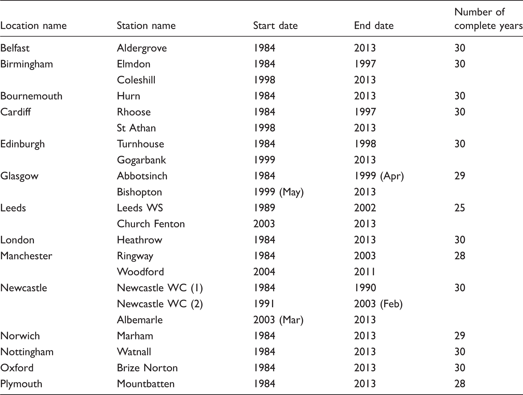
Even with selecting new weather sites to increase the number of observations available, there are still many holes in the BADC raw data which must be interpolated for use in the analysis. In this work, missing data are interpolated if less than 20% of the observations of dry bulb temperature for that month are missing, otherwise the month, and therefore the year is removed. If the weather is recorded on a bihourly basis, these data are interpolated even though only 50% of the total data are available. ¹⁴ Missing temperature data are interpolated in a four stage process. Firstly periods of data which are unlikely to contain a daily minima or maxima are flagged for interpolation. During the flagged periods, missing daily extrema are interpolated using valid points either side. Similarly, the hours at which these extrema occur are linearly interpolated. Finally, all other missing data are interpolated along with the generated minima and maxima using a spline algorithm.^3,15

Method

The weighted cooling degree hour and conceptual building overheating criteria

There are a number of ways in which overheating could be described. ⁸ The simplest candidate considers the number of hours which are greater than a threshold (e.g. hours over 28℃) as has been typically used to define overheating in schools. ¹⁶ However, while this is relatively simple to calculate and gives the total duration of the exposure it does not describe the severity. For example, if the threshold is 28℃, 40℃ would be considered an equal exceedance to 28.1℃. This is probably unrealistic and the former is clearly going to cause more discomfort. ¹⁷ Another candidate model is the cumulative hours above a threshold weighted by the temperature difference above the threshold (a degree hours definition). While this considers both the duration and the severity, it assumes a linear relationship between the exceedance and the level of discomfort which may be a simplification of the reality. It is likely that a temperature much above a given threshold is going to cause more discomfort than a temperature around the threshold. A third possibility weights the exceedance by the number of people dissatisfied given by a thermal comfort model. ⁷ Although this metric would have the closest match to reality, it is more complex than simply counting the number of hours over a threshold.

For each form of overheating, the internal temperature of a building as a response to the external conditions will be required so that the level of overheating can be calculated. Using the conceptual building, the external air temperature is equal to the internal operative temperature and a suitable comfort model must be considered. For free running buildings, BS EN 15251 suggests the use of adaptive thermal comfort model to assess comfort. ¹⁸ Using adaptive comfort criteria, the thermally neutral temperature is related to the daily running mean temperature which is given by

$T_c=0.33T_{\mathrm{rm}}+18.8$

(1)

where T_c is the predicted comfort temperature on a given day. T_rm is the daily running mean temperature which is given by

$T_{\mathrm{rm}}=0.8T_{\mathrm{rm}-1}+0.2T_{\mathrm{mean}-1}$

(2)

where T_rm−1 is the running mean temperature of the preceding day and T_mean−1 is the average temperature of the preceding day. Although Nicol et al. ⁷ developed an overheating metric using the thermal comfort concepts, ⁷ termed the potential daily discomfort, a simpler implementation of the approach can be considered, termed the weighted cooling degree hours (WCDH). ⁸ The weighting function in this case is then a quadratic expression given by,

$\text{WCDH}=\sum _{\mathrm{allhours}}\Delta T2$

(3)

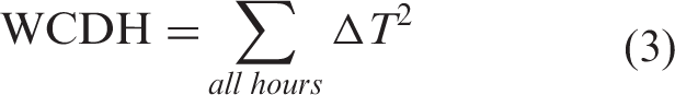
and

$\Delta T=T_{\mathrm{op}}-T_c,T_{\mathrm{op}}-T_c>0$

(4)

where T_op is the internal operative temperature. The weighting puts a much greater emphasis on operative temperatures which depart further from the comfort temperature. The WCDH approximation is related to the duration of the exceedance event as well as giving emphasis to more extreme temperatures which therefor takes into account the severity of the event.

Exploration of alternative overheating metrics

The original overheating metric analysis of TM49 (the ‘first metric’ considered above) was carried out in locations around the London area including Heathrow Airport, Gatwick Airport and London Weather Centre (central London). ⁸ These locations consist of some of the warmest in the UK with a high probability of this overheating metric being exceeded which will not necessarily be true of locations further north where the maximum temperatures are usually much cooler. A simple search through the available data shows that for London each year contained some degree of overheating above the comfort temperature; however, for Belfast, 8 of the 30 available years had no overheating as defined by this metric. To ensure the relative severity of overheating can be compared across all locations, a number of overheating metrics will be considered with results compared in addition to the WCDH as described above. The second metric will consider the weighted degree hours based on a static temperature threshold from which discomfort can be attributed. In the UK, a heat wave, as defined by the Met Office, depends on the location. In London, the threshold day time temperature is 32℃ where as in the North East this reduces to 28℃. 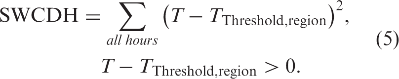¹⁹ However, it is apparent that excess deaths can begin to be attributed at much lower temperatures and can be attributed to the 93rd centile temperature at each region with strong statistical significance ²⁰ and therefore potential discomfort can occur at much cooler temperatures than the heatwave definitions. In this second metric, the WCDH will be calculated with the comfort temperature set to the 93rd centile temperature for that region for which the weather station is found, ²⁰ which in this case is a static temperature. This metric is therefore termed the static weighted cooling degree hours (SWCDH). The total for each location is therefore given by

$\text{SWCDH}=\sum _{\mathrm{allhours}}(T-T_{\text{Threshold},\text{region}})2,\mathrm{\hspace{1em}\hspace{1em}\hspace{1em}}T-T_{\text{Threshold},\text{region}}>0.$

(5)

The regional threshold temperature (T_{Threshold,region}) for each location is listed in Table 2. The original data exist for English and Welsh regions only so the thresholds for Northern Ireland and Scotland were inferred from the temperature distributions of these locations. The greatest correlation was found by linearly fitting the average summer daily maximum temperature at the location to the regional threshold. The threshold temperatures for Belfast, Edinburgh and Glasgow were then determined by evaluating the linear model with their average summer daily maximum temperatures.

Table 2.

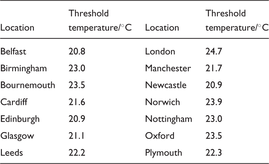
Temperature thresholds where excess heat related mortality occurs.

Location	Threshold temperature/℃	Location	Threshold temperature/℃
Belfast	20.8	London	24.7
Birmingham	23.0	Manchester	21.7
Bournemouth	23.5	Newcastle	20.9
Cardiff	21.6	Norwich	23.9
Edinburgh	20.9	Nottingham	23.0
Glasgow	21.1	Oxford	23.5
Leeds	22.2	Plymouth	22.3

The third metric combines the adaptation and comfort temperature of the WCDH metric with the regional threshold of method 2. This metric builds on the knowledge that regional mortality rates are correlated to different exceedance temperatures ²⁰ by reconciling with the first metric that discomfort is correlated to departures from the running average temperature. Furthermore, using adaptive comfort theory, it is currently recommended that the threshold for more vulnerable occupants is reduced. 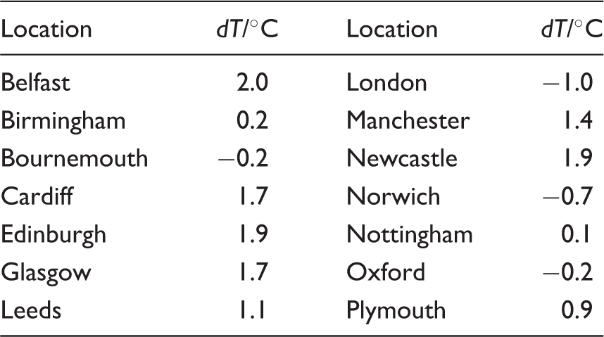¹⁸ This method considers that the comfort temperature threshold is also related to the location. For this metric, the threshold weighting degree hours (TWCDH) is given by

$\text{TWCDH}=\sum _{\mathrm{allhours}}(T-T_c+\text{d}T)2,\mathrm{\hspace{1em}\hspace{1em}\hspace{1em}}T-T_c+\text{d}T>0,$

(6)

where dT is the difference between the average comfort temperature calculated for all years over the summer months (April to September inclusive) at that location, and the regional threshold as per Table 2 at that location. The value of dT for each location can be seen in Table 3. A positive value for dT has the effect of lowering the adaptive comfort temperature, while a negative value increases the adaptive comfort temperature, suggesting that occupants would be comfortable at a higher threshold at these locations. The value of dT is negatively correlated (R²= 0.9) with the average daily summer maximum temperature.

Table 3.

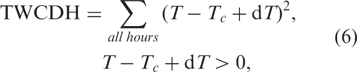
Difference between a locations average summer (April to September) comfort temperature across all years and the regional 93rd centile temperature threshold where excess heat related mortality occurs.

Location	dT/℃	Location	dT/℃
Belfast	2.0	London	−1.0
Birmingham	0.2	Manchester	1.4
Bournemouth	−0.2	Newcastle	1.9
Cardiff	1.7	Norwich	−0.7
Edinburgh	1.9	Nottingham	0.1
Glasgow	1.7	Oxford	−0.2
Leeds	1.1	Plymouth	0.9

Estimating return periods of warm summers

The return period of an event refers to the frequency of the event with an associated exceedance value. The original DSY methodology considered the third hottest summer on the basis of average April to September temperature from a base period which was up to 21 years in length. This means that, assuming the current climate has no underlying trend, any given future summer has a 1-in-7 chance of being equal or hotter than the selected DSY ⁴ or such a summer has a return period of seven years. The original DSY selection also assumes that each year is equally likely. The mean temperature in any given year could be described as a random event and could take a range of values. However, years which have a mean temperature similar to the overall mean should occur more often and therefore have a higher probability of occurrence associated with it. To provide a better estimate of the underlying distribution of the mean temperature, it is possible to fit different classes of functions to the data.

The generalised extreme value (GEV) distribution ²¹ is frequently applied to climatological data to model the most extreme value within a period such as the extremes of rainfall ²² or to evaluate the effects of climate change. ²³ To describe the statistics of rare events, the GEV approach estimates the return period of these extreme events. Assuming the observed threshold events are independent and uniformly distributed the probability density function of a set of events (x, such as SWCDH) is given by

$f(x|k,\mu ,\sigma )=\{(\frac{1}{\sigma })\exp (-\exp (-\frac{x-\mu }{\sigma })-\frac{x-\mu }{\sigma }),k=0(\frac{1}{\sigma })\exp (-(1+k\frac{x-\mu }{\sigma })-\frac{1}{k})(1+k\frac{x-\mu }{\sigma })-1-\frac{1}{k},k\ne 0,1+k\frac{x-\mu }{\sigma }>0,$

(7)

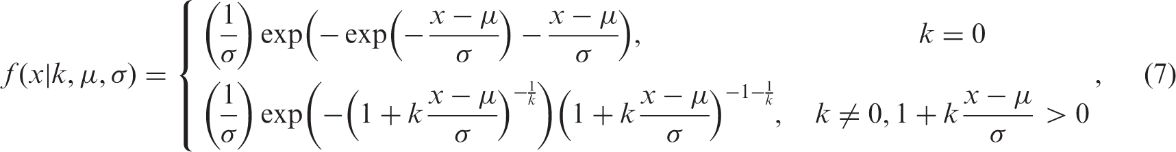
where µ is the location parameter, σ is the scale parameter and k is the shape parameter. The events are typically fitted to the distribution using a maximum likelihood estimator method, as used by Matlab. ²⁴ The T-year return values X_Tgev are then estimated from,

$X_{\mathrm{Tgev}}=\{\mu -\sigma \ln [-\ln (1-\frac{1}{T})],k=0\mu -\frac{\sigma }{k}(1-[-\ln (1-\frac{1}{T})]-k),k\ne 0,.$

(8)

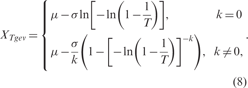
Within this analysis, the threshold events will be the data generated for each metric and the period will be one year.

Although the GEV theory is straight forward to apply, the use of a yearly value may result in extensive data reduction. For example, in this work for a given year we are interested in the sum of all temperatures which are extreme deviations from a comfort temperature. For locations which are inherently colder, typically further north, there is a high probability that there is little or no overheating if the threshold is too extreme. In this case, the large number of ‘zero’ events would have the greatest influence on the distribution, while years which have a number of independent overheating events are summed to produce a single value. While this has been considered by using more than one comfort threshold to carry out the analysis, the generalised Pareto distribution (GPD), or peak over threshold method, could be used as an alternative. Using the GPD, each individual exceedance event is included as a separate entity (rather than modelling a single peak value) so there are more extreme events in the analysis^25,16 allowing the calculation of the return periods for the individual events. The key aim of this work is to determine the severity of warm temperatures by assigning return periods to the events. This in turn will allow the selection of PDSYs to inform practitioners of the risk of overheating of their building design. However, selecting a year from individual events with particular return periods is less straight forward. It is likely that for a given year that more than one event could exist with different return periods. As these return periods are independent from each other, no correlation can be generalised from the distribution of these events. A simple solution may be to once the year has been selected from an event at a given return period to exclude it from further analysis. However, this still leaves the dilemma when determining what is a more extreme year; for example, is a year with two events each with return periods of 1 in 20 years less or more severe than a year with a single 1 in 25 years event? If this approach is taken there is a strong possibility that industry could find that for what is determined a more frequent, less extreme year to have much more overheating than a more extreme year leaving industry no better off than before this exercise. An alternative would be to consider that all overheating events in a given year are dependent on each other. This would give a maximum number of events equal to the maximum number of years in the baseline. This is equivalent to fitting the GPD to the original data set for all years where the total is greater than 0. However, this approach is likely to violate the criteria that the events should be independent with a frequency given by a Poisson process as most years would be used in this analysis. ²¹ Furthermore, even using this technique it is likely that too few data points would be included to ensure accuracy of the fitted GPD.

The GPD is highly suitable for determining the return periods of the individual events contained within a dataset, there are potential difficulties of extending the analysis to determine the return periods of a contiguous year which can be used in building simulation. To establish PDSY and assign appropriate return periods, the most robust approach is the GEV distribution fitted to the sum of the metric for the year and will be used in the following analysis.

Results

Extreme value analysis and return periods of events

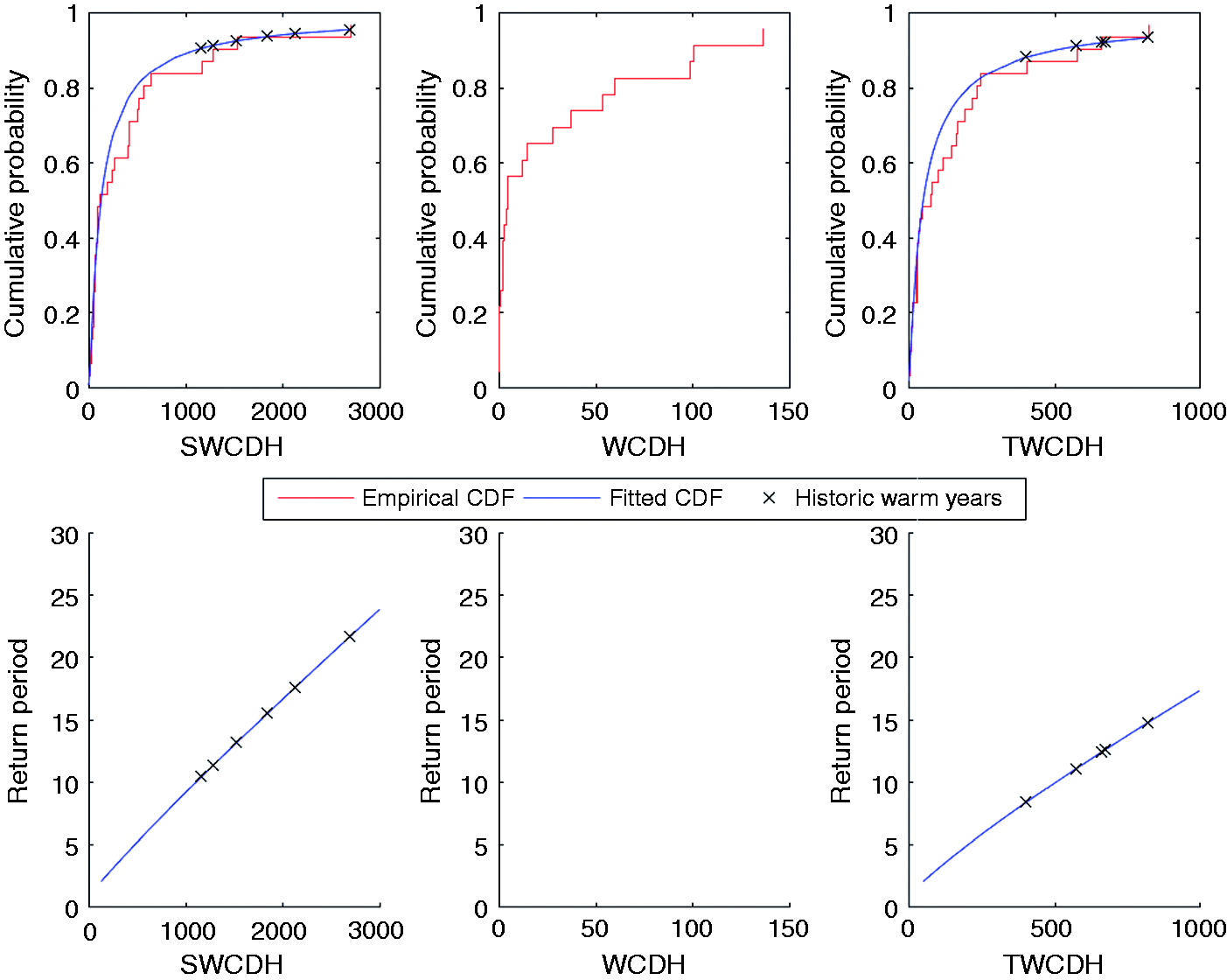
The results of the return period analysis for all three overheating metrics as described above for London and Belfast are shown in Figures 1 and 2 and Tables 4 and 5, respectively. The empirical and fitted GEV cumulative distributions for the years 1983–2013 and the calculated return periods for each metric for each location are shown in Figures 1 and 2 demonstrating the goodness of fit. The GEV distribution in each case is used to calculate the return periods of all available years from 1961 and all historic warm periods are marked then. The 10 warmest years ranked according to the SWCDH metric for all three overheating metrics are listed in Tables 4 and 5 along with the return periods of the locations TRY. The TRY year is created using the same updated baseline (1984–2013) and then using the method of Eames et al. ²⁶

Figure 1.

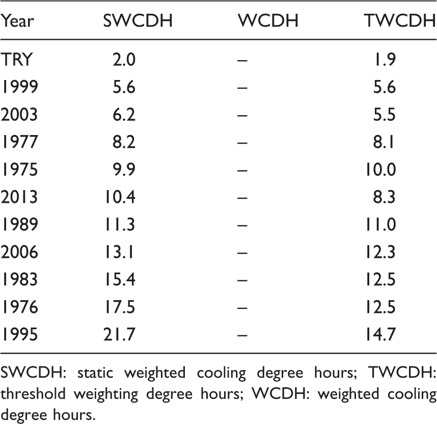
Return period analysis against SWCDH, WCDH and TWCDH for London. The locations of historic warm summers are also shown by crosses.

Figure 2.

Cumulative probability and return period analysis against SWCDH, WCDH and TWCDH for Belfast. The locations of historic warm summers are also shown by crosses.

Table 4.

Yearly return periods for all overheating metrics for the ten warmest years for London ordered by the number of SWCDH. The return period of the TRY is also shown.

Year	SWCDH	WCDH	TWCDH
TRY	2.0	2.0	2.1
2005	4.9	6.5	6.5
1975	6.2	5.1	5.1
1989	6.7	6.8	6.1
2013	6.8	5.9	6.0
1983	7.6	5.4	5.2
1990	11.7	12.5	12.3
2003	15.5	15.5	15.0
2006	15.6	16.0	14.1
1995	15.9	14.8	12.5
1976	23.7	22.2	18.9

SWCDH: static weighted cooling degree hours; TWCDH: threshold weighting degree hours; WCDH: weighted cooling degree hours; TRY: test reference year.

Table 5.

Yearly return periods for all overheating metrics for the ten warmest years for Belfast ordered by the number of SWCDH. The return period of the TRY is also shown.

Year	SWCDH	WCDH	TWCDH
TRY	2.0	–	1.9
1999	5.6	–	5.6
2003	6.2	–	5.5
1977	8.2	–	8.1
1975	9.9	–	10.0
2013	10.4	–	8.3
1989	11.3	–	11.0
2006	13.1	–	12.3
1983	15.4	–	12.5
1976	17.5	–	12.5
1995	21.7	–	14.7

SWCDH: static weighted cooling degree hours; TWCDH: threshold weighting degree hours; WCDH: weighted cooling degree hours.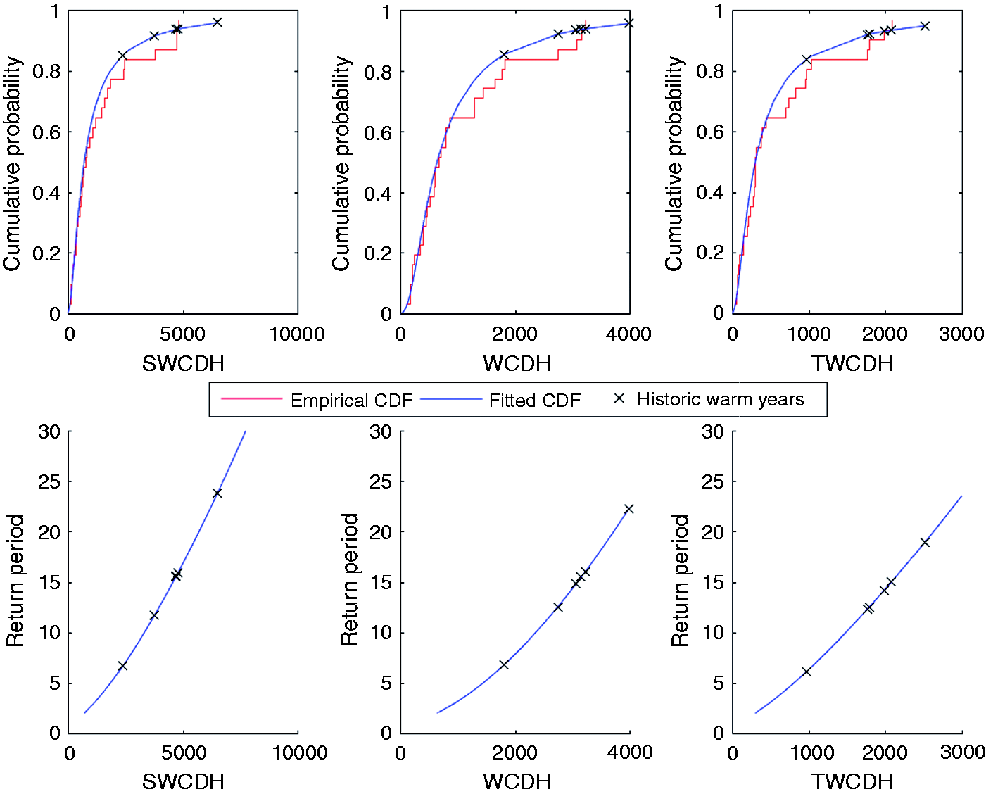

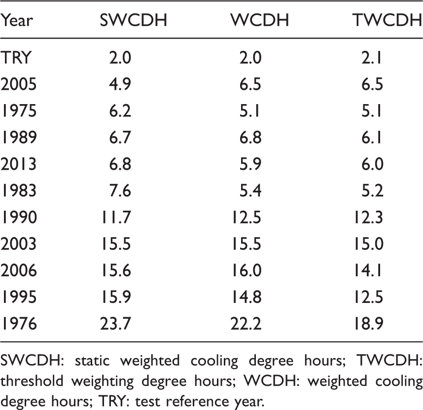
The analysis shows that for London the DSY established in 2006 (1989) can now be defined as having a return period of 6.7 years using the SWCDH metric, 6.8 years using WCDH metric and 6.1 years using the TWCDH metric (Table 4). Overall the order of the years is dependent on the metric used but the hottest years (1990, 2003, 2006, 1995 and 1976) remain the hottest years with return periods of the order of 11.7 to 23.7 years.

The analysis shows that for Belfast there is not enough data to fit the GEV distribution to the WCDH metric (Table 5). There are eight years from the baseline which have no WCDH data with most years having very few exceedances above the comfort temperature threshold dominating the GEV analysis. For the SWCDH and TWCDH metrics, the return periods were calculated as between 5.5 and 21.7 years for the 10 warmest years, similar in magnitude to the London return periods. The hottest years by the two remaining definitions remain the hottest years although in this case the 2013 moves from sixth hottest for SWCDH to seventh hottest using TWCDH.

Tables for all locations as listed in Table 3, similar to Tables 4 and 5, can be found in the Appendix. Overall the TRY years at each location are found to have return periods which range from 1.3 years to 5.6 years. The vast majority of the TRYs have return periods of less than four years.

It must be noted that the error in the estimated return periods increases as the return period gets greater. For return periods of the order of 3 or less years, a 90th percentile confidence interval is of the order of 0.4 years, for 7-year return period the interval increases to 2 years and for a 23-year return period the interval increases to the order of 7 years. For the extreme cases such as a return period of 50 years as found for Norwich, the 90th percentile confidence band is 20 years. The confidence intervals are always positively skewed giving much greater confidence in the lower return periods.

Choosing PDSYs

The previous methodology used to create DSYs considered a moderately warm summer as the third hottest from a typically 21 years implies a return period of 7 years. ³ For many locations much less complete data were available, ⁴ while maintaining the third hottest requirement. This would have the consequence of reducing the return period for the effected locations but this was not the original intention of the method. A moderately warm event year will be considered as the year with a return period closest to seven years similar to the original intention of the DSY methodology. However, the use of return period analysis removes the requirement that all data for all locations need to be available. It is clear from Tables 4 and 5 (and the Appendix) that the definition of a 1 in 7 years depends on the metric chosen. For example, for London, the candidate years are 2013 (SWCDH), 1989 (WCDH) and 2005 (TWCDH). Similarly for Belfast, the candidate years are 2003 (SWCDH) and 1977 (TWCDH). To get a better understanding, a closer examination of the three metrics is required. The SWCDH is a weighted measure of the number of hours above a temperature threshold which has been determined as the point at which adverse effects started. The weighting gives stronger influence to temperatures which are further from the threshold temperature. The WCDH metric is the weighted measure of the number of hours above an adaptive comfort temperature. In this case, exceedances above the comfort temperature put emphasis on rapid changes in the weather. The TWCDH metric is similar to the WCDH metric but includes an offset to take account of the regional effects as outlined in Table 3. From Table 2 and equation (1), the threshold temperature for the WCDH metric is more extreme than the regional threshold used to calculate the SWCDH. The TWCDH metric is a regionalised, slightly less extreme measure of overheating than the WCDH metric but again still puts an emphasis on rapid changes in recent weather. The SWCDH is a regionalised threshold based on the point at which a risk to occupants due to temperature starts to appear so, the candidate moderately warm summer year can be considered as the year with the SWCDH return period of seven years (or the year with the return period closest to seven years). For London, the moderate DSY (DSY-1) is 2013 and for Belfast the year is 2003. Note the London moderate DSY is different from that selected in TM49 but according to Table 4 there is little difference between 2013 and the TM49 year of 1989.

This single PDSY does not capture the entire risk to the building occupants as different people will have different thermal responses to different warm weather events. Where the occupants of a building are more vulnerable, these warmer summer conditions must be considered. TM49 defined two more extreme overheating events with different characteristics. ⁸ The first is a year with a long period of persistent warmth and the second is a year with a shorter more intense warm spell. For the purpose of this analysis, these candidate years must also be more extreme in terms of WCDH return periods (where available) and TWCDH return periods.

The characteristics of the 10 warmest spells for London are listed in Tables 6, 7 and 8 ordered by SWCDH, WCDH and TWCDH, respectively. A warm spell has been defined as a continuous period where at least 1 h of each day goes above the respective threshold temperature. Warm spells which are separated by up to three days are counted as the same warm spell. The intensity is simply the total of the metric divided by the number of days of the event. All of the warm spells occurred in June, July and August with the majority starting in July. The same years appear in all three tables but the order of the warm spells depends on the metric demonstrating the difficulty of selecting a single year to reflect the risk to overheating or selecting more intense years.

Table 6.

Characteristics of the ten warmest events ordered by the total SWCDH for London.

Start date	SWCDH	Duration/ days	SWCDH intensity
22 June 1976	5754	28	206
2 August 2003	3921	17	231
18 July 1995	3852	39	99
11 July 2006	3136	20	157
25 July 1990	2411	11	219
2 July 1983	2396	30	80
26 July 1975	2167	20	108
05 July 2013	1788	24	74
15 July 1989	1551	15	103
29 June 2006	956	8	119

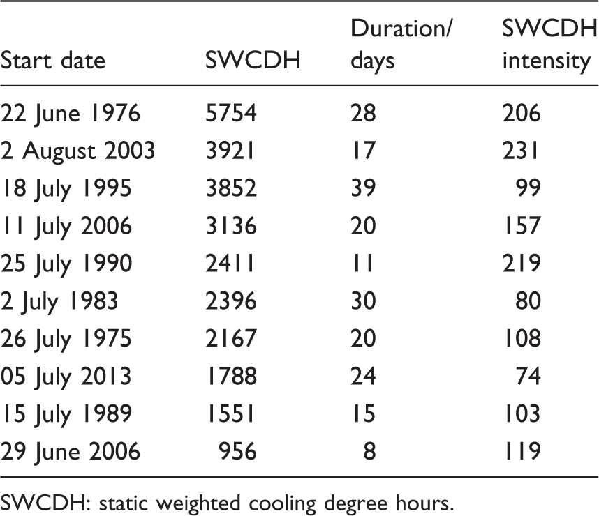
SWCDH: static weighted cooling degree hours.

Table 7.

Characteristics of the ten warmest events ordered by the total WCDH for London.

Start date	WCDH	Duration/ days	WCDH intensity
22 June 1976	3232	21	154
02 August 2003	2471	12	206
12 July 2006	1855	17	109
31 July 1990	1656	5	331
26 July 1975	1260	14	90
02 July 1983	1106	17	65
05 July 2013	1104	23	48
29 July 1995	1055	9	117
15 July 1989	961	15	64
10 August 1995	758	13	58

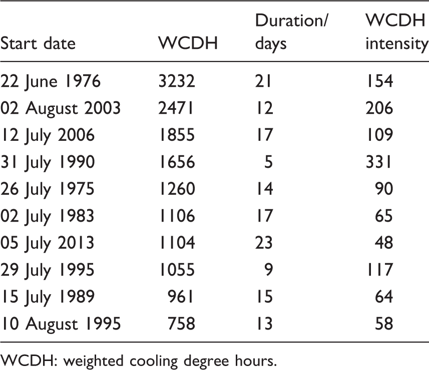
WCDH: weighted cooling degree hours.

Table 8.

Characteristics of the ten warmest events ordered by the total TSWCDH for London.

Start date	TWCDH	Duration/ days	TWCDH Intensity
14 June 1976	2128	21	101
12 August 2003	1754	11	159
12 July 2006	1213	13	93
16 July 1990	1208	5	242
14 July 1975	769	13	59
11 July 1995	682	6	114
15 July 1983	641	16	40
15 July 1989	591	11	54
10 July 2013	548	11	50
15 June 2006	446	6	74

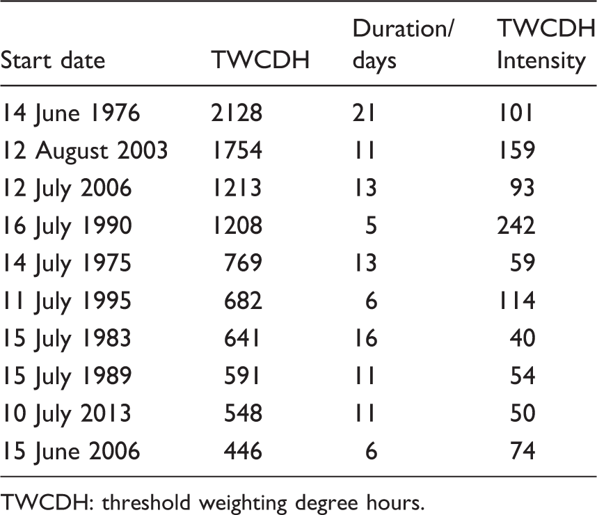
TWCDH: threshold weighting degree hours.

From Table 4, there are six years which have a larger return period compared to 2013 in terms of SWCDH for London. The features of these six years will be examined more closely: It is clear that longest 1976 event is longer in duration than that of 2013 and is approximately two to three times more intense for each metric; 1983’s warmest event, although longer in duration than 2013 in terms of SWCDH is less intense for the TWCDH and shorter for the WCDH; 1990 has a single very short very intense event; 1995’ss warmest event is very much less intense in terms of SWCDH but very much longer than the warmest 2013 event and in the more extreme metrics (WCDH and TWCDH) the event is not particularly long; 2003 has an event which is approximately the same duration or shorter than 2013, depending on the metric but is much more intense in every metric; 2006 has an event which is similar to 2003, but is much less intense.

On the basis of this analysis, 2003 is selected as the second PDSY; the SWCDH return period is just over double that of 2013 (Table 4) and the duration of the warmest event is similar to 2013 but is more intense in every metric (Tables 6, 7 and 8). Similarly, the third PDSY is selected as 1976; the SWCDH return period is just over three times that of 2013. In this case, the duration of the warmest event of 1976 is much longer in duration than both 2003 and 2013 but is also less intense than 2003 and simultaneously more intense than 2013.

Following this analysis, PDSYs can be selected for all locations as listed in Table 9. The moderate event DSY is defined as the year with the SWCDH return period closest to seven years. The more extreme summer years are then determined. The intense extreme year is chosen as the year with the event which is about the same length as the moderate summer year and has a higher intensity than the moderate summer. The long extreme year is determined by the year with a less intense event than the high intensity year, more intense event than the moderate summer year but also has a longer duration than the moderate summer year. The more extreme DSYs must all have a greater return period in terms of SWCDH than the moderate DSY. For some locations, the selection of the PDSYs is less straight forward so further details on the selection criteria for each location are presented in detail in the Appendix.

Table 9.

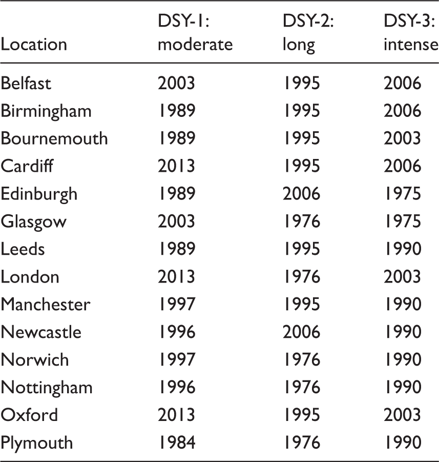
Probabilistic design summer years for all locations.

Location	DSY-1: moderate	DSY-2: long	DSY-3: intense
Belfast	2003	1995	2006
Birmingham	1989	1995	2006
Bournemouth	1989	1995	2003
Cardiff	2013	1995	2006
Edinburgh	1989	2006	1975
Glasgow	2003	1976	1975
Leeds	1989	1995	1990
London	2013	1976	2003
Manchester	1997	1995	1990
Newcastle	1996	2006	1990
Norwich	1997	1976	1990
Nottingham	1996	1976	1990
Oxford	2013	1995	2003
Plymouth	1984	1976	1990

Discussion and conclusion

The method described in this work assigns return periods for warm weather events using three definitions of overheating: the SWCDH with the threshold given as the 93rd centile temperature for the region of the weather station; the weighted cooling degree hours with the threshold given as the comfort temperature; and the threshold weighted cooling degree hours where the threshold is adjusted from the comfort temperature according to the region. The moderate event DSY was defined as the year with the SWCDH return period equal to (or closest to) seven years. The more extreme summer years were then selected on the basis that they were both more extreme than the moderate year and consisted of overheating events with a different character (either of longer duration and more intense or of about the same duration but much more intense). The method ensures that the moderate summer is consistently defined across the UK and that the more extreme events at each location have a clear relative definition for that location. This methodology ensures that point 1 as detailed in the background – the severity problem – and by Jentsch et al.^4,5 is addressed.

For the moderate DSY, the year selected in each case ranged from the 10th hottest (Plymouth) to the 4th hottest (Leeds) on this metric. In this case, the use of a return period to choose a year is not to find the nth hottest year from a set of years, but to choose a year which has the same probability of occurrence at each location. The GEV distribution is fitted to the meteorological normal period of 1984–2013 and then this distribution is used to establish return periods for all available years since 1961 (depending on location). For Leeds, the data are only available from 1989 for both parts of this analysis so it is consistent that the chosen year is the fourth hottest out of 25 years compared to the average across all locations of eighth hottest out of 48 years. For the more extreme years, there are strong correlations between all locations. Four possible years are selected for the intensive extreme year (1975, 1990, 2003 and 2006), whereas three years are selected as the long extreme year (1976, 1995 and 2006). Interestingly, 2006 is a shorter intense extreme year for Birmingham, Belfast and Cardiff but becomes a longer less extreme event for the more northern locations of Newcastle and Edinburgh.

The corresponding TRY files are less extreme than the chosen DSYs years for all locations as listed in Tables 4, 5 and the Appendix in terms of the SWCDH and TWCDH. In each case, the TRY has a maximum return period of 5.6 years. It may be expected that the equivalent TRY file would have a return period of the order of 2 years given that it is supposed to represent the average yearly conditions. However, the TRY months consist of the most average temperature, solar radiation (by means of average cloud cover), relative humidity with the use of wind speed as a secondary variable and so it is of no surprise that the return periods are slightly higher than the expected two years. The metrics used to determine the PDSYs give preference for a series of days which are warm, whereas the TRY methodology gives preference for days which are average, but may still contain a warm/hot day. On closer examination of the files, there are three locations where the peak TRY temperature is similar but greater than a peak PDSY temperature (Cardiff, Leeds and Norwich) equivalent to the peak temperature or one warm day. For these locations at least the next 28% (and up to 100%) of all temperatures within the DSY file are warmer than the TRY file. This approach has helped with point 2 as detailed in the background – the temperature problem. The use of observations might limit the ability for this issue to be eliminated completely if desirable and the use of mathematical transformations would then be required. ⁵ Furthermore, as stated above, the TRY selection criteria do not disallow the selection of hot days.

This issue may not necessarily be an issue for this set of weather files. The various warmest days within the TRY files form part of warm periods which lasts at most two days. Within each PDSY, the peak temperature is found amongst a number of warm days which could increase the likelihood of overheating when used in building simulation – the building fabric might already be spun up to a warmer state before the warmest period occurs. For all weather files, return periods of the years have been determined which allows the level of overheating to be put into perspective. Although a reference building was used to determine the PDSYs and predict overheating to deal with point 3 as detailed in the background – the overheating problem, verification is still required as to the extent to which these years can be used to determine overheating in real building models.

A consistent set of probabilistic weather years have been produced for all locations but the statistical methods used are based entirely on the external temperature and ignore the effect of solar radiation. While this is might be an issue for heavily glazed buildings, it is clearly impossible to create a conceptual building which can account for all forms of glazing. It is unlikely that the solar radiation is consistent across the set of moderate event years as this considers the peak above the lowest threshold considered. However, the more extreme years are more likely to be consistent with warmer spells which contain longer high pressure systems, which bring warmer temperatures, clearer skies, longer solar duration and thus more solar radiation. With both warm intense events and shorter much more intense events considered a range of overheating events can be investigated during building design.