
Abstract
Systematically missing information on secondary respondents is a frequent problem in multiactor surveys. Budget and time constraints often prevent all variables collected for primary respondents (e.g., anchors) from being collected for secondary respondents (e.g., partners). Thus, a subset of variables are systematically missing for secondary respondents. This can severely limit the analysis potential of multiactor data, ruling out all research questions that would require (the same) information on primary and secondary respondents. The problem of systematically missing data is also present in other settings, for example, after changes in measurement instruments in repeated surveys or in ex post survey harmonization if one or more surveys did not include a specific variable. In these cases, using multiple imputation (MI) techniques to impute the missing variables is a common approach. The authors explore whether MI can be used when data on secondary respondents are systematically missing. Results from simulation studies show that imputation under the assumption of conditional independence for primary and secondary respondents variables leads to a strong bias toward zero in the estimated partial correlation between primary and secondary respondents. However, external data in the form of bridging studies can be used to estimate the partial correlation between the observed variable for the primary and the unobserved variable for the secondary respondent, leading to estimates with less bias after MI.
Keywords
Multiactor studies collect information on persons who maintain a significant relationship or connection with each other. For analyses of couples or romantic relationships, for instance, the anchor respondent’s partner can be included as a “secondary” respondent in a multiactor survey (Dykstra et al. 2012; Kalmijn and Liefbroer 2010; Kalmijn et al. 2018). 1 However, questionnaires for secondary respondents may not include all items collected for anchors (Brüderl et al. 2017; Dykstra et al. 2012). This can be due to the general challenges faced by all (large-scale) survey programs: increasing demands coupled with reduced resources. It is also not uncommon in multiactor surveys that interview modes for secondary respondents differ from those of the anchors, which can lead to a smaller set of variables being collected for those respondents. Taken together, these constraints in data collection often lead to specific variables being recorded only for anchors but not for their partners. This is a case of systematically missing data (Resche-Rigon et al. 2013), as some data are unavailable for all secondary respondents.
In this article, we addresses this challenge from the perspective of data integration (Yang and Kim 2020) or data fusion (Rässler 2003) by investigating if an auxiliary data set—a “bridging study” 2 (Parker et al. 2004; Schenker and Raghunathan 2007)—or auxiliary information (Moretti and Shlomo 2023) can be used in combination with multiple imputation (MI) (Resche-Rigon et al. 2013) to address the problem of systematically missing partner information in multiactor survey data. Data integration is an emerging area of research that departs from a traditional study-centric approach to using data from multiple sources (Kim et al. 2021). The approach is promising because it can reduce costs associated with surveys, reduce respondent burden, and allow investigation of a broader set of research questions (i.e., by imputing unobserved confounders) that cannot be addressed by a single study alone (Yang and Kim 2020).
Although this article is the first to examine whether techniques of MI, which are extensively used to impute partially missing data (van Buuren 2007), can be used to address the problem of systematically missing information in multiactor surveys, these methods are already used to address similar problems. Current applications range from imputing missing confounders in a meta-analysis of individual person data (IPD) (Resche-Rigon et al. 2013) to imputing missing variables in split-questionnaire designs (Rässler 2003), bridging old and new measures in repeated surveys (Parker et al. 2004; Schenker and Raghunathan 2007), and combining probability and nonprobability samples (Kim et al. 2021).
Systematically missing information for secondary respondents presents a structurally similar problem. However, a particular challenge in anchor-partner data is that of similarity between anchor and partner, for example, homogamy (Kalmijn 1998). We can derive two possible approaches from the literature in related fields. The first approach is to assume that the partial correlation between the systematically missing partner variable and its corresponding anchor variable, given other jointly observed variables, is zero. This assumption is also called the assumption of conditional independence (Resche-Rigon et al. 2013). The second approach is to estimate the (partial) correlation in another study, that is, a bridging study (Parker et al. 2004), in which the variable of interest is observed for both primary and secondary respondents. This approach requires the assumption that the estimates from the bridging study are transferable to the original study with the systematically missing partner variable. We pioneer a novel third approach, wherein we assign plausible values for the partial correlation, drawing on those observed in bridging studies or in the literature. This step forms the bedrock for our distinctive method of MI. We evaluate these strategies to give insight into whether they are suitable for the imputation of systematically missing variables for secondary respondents.
The article is structured as follows. First, we briefly overview MI principles for missing data. Second, we review previous research on systematically missing data, focusing on approaches that aim to resolve this problem through MI. We briefly introduce each area and summarize the critical differences in the pattern of systematically missing data. Third, building on this literature, we outline MI approaches for systematically missing data for secondary respondents. We illustrate the approaches through a simulation with data from the German Socio-Economic Panel (GSOEP) (Goebel et al. 2019), the German Family Panel (pairfam) (Brüderl et al. 2017), and the German sub-study of the Survey of Health, Ageing and Retirement in Europe (SHARE) (Börsch-Supan 2020; Börsch-Supan et al. 2013). After presenting the results of the simulation, we discuss how study heterogeneity can affect the performance of MI.
Literature Overview: Systematically Missing Data in Related Fields
The term systematically missing data was coined for meta-analysis with raw data, also called IPD meta-analysis (Resche-Rigon et al. 2013). In an IPD meta-analysis, raw data from several studies are combined and then jointly analyzed. In the social sciences, research projects combining, pooling, and harmonizing data are usually not called IPD meta-analyses, but instead described as ex post survey harmonization projects (Granda, Wolf, and Hadorn 2010) or simply combining or merging data (e.g., Broege et al. 2007; von Hippel, Scarpino, and Holas 2016). If an analysis were to be conducted only with one data set with a systematically missing variable, it would not be possible to include the systematically missing variable. For example, in Figure 1, variable 1 is not observed for studies 5 and 6, but it is in all other studies. This would hinder joint analyses. However, the studies in which variable 1 is observed can be used as “bridges” to impute the data in Studies 5 and 6.
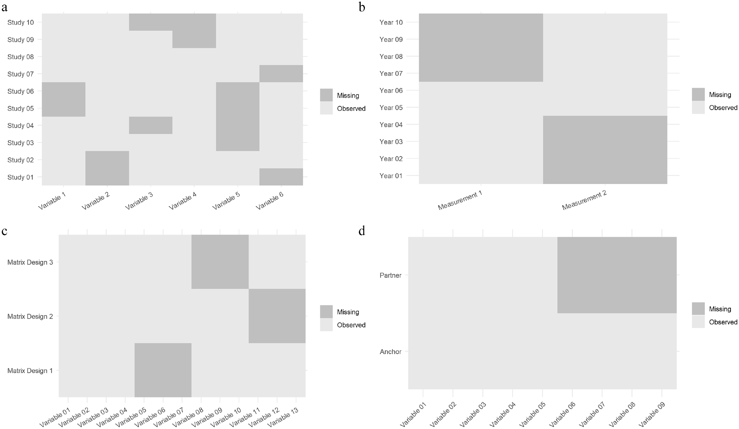
Systematically missing data in different cases: (a) survey harmonization, (b) official statistics with changing measurements, (c) split questionnaire/matrix design, and (d) partner variables.
Systematically missing data can also occur in official statistics if measurements change over time (Parker et al. 2004; Schenker and Raghunathan 2007), that is, between waves of a panel or for a time series (see Figure 1b). The change in measurements hinders comparisons over time. However, both measurements can be included in a survey for a limited period. This time period then serves as a bridging study, allowing the creation of a complete timeline for either of the measures.
A similar situation arises in split questionnaires, also called matrix design (see Figure 1c), in which the questionnaire is split into several modules. Split questionnaire design is used to reduce respondents’ burden and survey costs (Rässler 2003), as respondents are only asked varying subsets of modules (see Figure 1c). After data collection, missing components can be imputed. Each split serves as a “bridging study” for other splits in the same questionnaire. In both “bridging studies” and split questionnaire designs, the researcher can typically control which variables are observed together (for more information regarding the implementation of optimal matrix designs, see Adigüzel and Wedel 2008; Raghunathan 2006).
The comparison of the different areas in which systematically missing data appear reveals differences and similarities (see Figure 1 and Table 1). For example, the respondents’ grouping varies by year of survey in the case of bridging studies, by study in the case of survey harmonization, and by matrix subset in split questionnaires. Another important difference is the level of similarity between the study or the studies with systematically missing data and the bridging study. One of the greatest challenges for data integration, combining information from multiple sources, is that of incomparability (Dong, Elliott, and Raghunathan 2014; Roberts and Binder 2009). Ideally, a bridging study should be as similar as possible to the original study with respect to the (1) underlying population, (2) sampling, (3) interview mode, and (4) measurements, as the bridging study and its data structure are used to extrapolate the relationship between the systematically missing variable and the other variables in the main study. In official statistics and split questionnaires, changes in study designs present optimal imputation situations, compared with survey harmonization, because one has control over the underlying population and sampling, mode, and measurements. Comparing systematically missing information from partner respondents with other cases of systematically missing data, we first notice that data are missing for the partners (see Figure 1d). A subset in which the variables are observed for both anchor and partners does not exist. Therefore, we need to make either an additional assumption concerning the (conditional) dependence between observed and unobserved variables or rely on an external data set, which can serve as a bridging study for MI.
Comparison of Different Problems Related to Systematically Missing Data.
One, but not the only, important potential application case is panel studies, where data are collected over multiple waves, and certain variables may not be included in all waves. This is especially true because of the significant effort required for partner interviews. In the German family panel pairfam, many variables about partners are only surveyed every two years, in contrast to the annual surveys for anchor respondents. The comparison with bridging studies in official statistics also helps illuminate why simply using the bridging study as the data for the substantive analysis the researcher is interested in is not always an option. Researchers might be interested in data belonging to different samples or years and only need the bridging study to fill in the gaps. The bridging study might be smaller in scale, thus resulting in less power, or might be missing other variables needed for analysis (for which we would need a bridging study again).
Motivational Example: Life Satisfaction of Partners in Germany
To illustrate and empirically test our approach, we build our simulation on a simple example where we assume we have a multiactor survey—anchor and partner—in which some information for the partners is systematically missing. We assume we need information on both the anchors’ and the partners’ life satisfaction, but it is observed only for the anchors. Naturally, it depends on the specific research question at hand whether information on the partner’s life satisfaction is needed. We use auxiliary information (Moretti and Shlomo 2023)—a bridging study—in combination with MI (Resche-Rigon et al. 2013) to impute the missing information. This is intended only to serve as an illustrative example; the approach might be useful in other contexts as well.
In our motivational example, we estimate the (partial) correlation between the partner’s life satisfaction and the anchor’s life satisfaction while controlling for sociodemographic characteristics and the Big Five personality traits of the anchor and partner. Although all covariates are available for anchors and partners in the original data, we treat partners’ life satisfaction as systematically missing to evaluate different imputation strategies. We use the GSOEP (Goebel et al. 2019) as our primary study and, as bridging studies, pairfam (Brüderl et al. 2017) and the German substudy of SHARE (Börsch-Supan 2020; Börsch-Supan et al. 2013). Although the surveys are longitudinal, we use the data purely cross-sectionally, that is, only one wave from each study.
A challenge in imputing systematically missing partner data lies in the potential interdependence of persons within partnerships. Similarities or dissimilarities in life satisfaction between partners can exist for many reasons, for instance, through assortative mating, shared experiences, mutual influence, competition, or task sharing (Byrne 1971; Dyrenforth et al. 2010; Gustavson et al. 2016; Kenny and la Voie 1985; Ledermann and Kenny 2012; Schade et al. 2016). As we discuss in the next section, how we deal with anchor-partner dependence is central to the imputation strategy and whether we need a bridging study or auxiliary information.
Imputation Strategies for Systematically Missing Partner Variables
MI
One of the most popular approaches to tackling missing data is MI (Little and Rubin 2002). MI allows the analysis of incomplete data sets by substituting missing values. We replace them by “imputing” values of a variable conditioned on other variables; in general, conditioned at least on the variables of the substantial analysis model (Carpenter and Kenward 2013:72). This procedure is repeated several times, creating several data sets. Each data set is analyzed separately, and estimates are combined across imputations using rules developed by Rubin (1987). One major advantage of MI approaches over single imputation approaches is that the former gives unbiased variance estimates.
To impute missing values, we need models specifying the distribution of the missing values. There are two main approaches, joint modeling (JM) (Schafer 1997) and the fully conditional specification (FCS) (van Buuren et al. 2006). In JM, missing values are drawn simultaneously for all incomplete variables using a multivariate distribution. FCS is known under a multitude of names, for example, as MI by chained equations (mice). In contrast to JM, FCS “splits” the problem into a series of univariate problems (van Buuren 2007). FCS involves specifying each partially observed variable’s conditional distribution through a series of univariate models, given all the other variables (White, Royston, and Wood 2011). Imputation under FCS is then done by iterating over the conditionally specified imputation models. FCS is more flexible than the JM approach because we can select adequate regression models for every variable (e.g., linear regression for continuous partially observed variables, logistic regression for binary partially observed variables). An important weakness of this approach is that the specified conditional densities can be incompatible. Thus, we possibly do not know the joint distribution to which the imputation algorithm converges. However, in practice, the approach’s actual performance is often good (van Buuren 2007).
Because of its popularity and flexibility, we use FCS to test the different approaches. Given our aim here is to explore whether the use of bridging studies is a possible remedy for systematically missing partner variables in general, we do not compare different imputation packages. Instead, we restrict ourselves to one of the most popular ones (mice in R [R Foundation for Statistical Computing]). 3 The Appendix provides a description of the algorithm for imputing with a bridging study. To combine the estimated correlation coefficients after imputation, we use the micombine function from the package miceadds. The approaches tested can also be carried out with other FCS imputation packages or transferred to JM approaches.
MI for Systematically Missing Partner Variables: Assumptions and Bridging Studies
We first include the full GSOEP data set (marked as “01. Full data set” in the results and figures) before deleting the partner variable for comparison and reference. For a detailed description of the data set, see the section “Data Sets: GSOEP, SHARE and pairfam.”
For the imputation approaches, we start with the least complex ones and move up to the possible inclusion of bridging studies in the imputation procedures. A simple way to impute the missing data is to impute in long format, that is, with the information on anchors and partners in separate rows (Figure 2a). However, this imputation approach (“02. MI in long format”) completely ignores possible dependencies between anchors and partners in a relationship. The approach will work only if the partial correlation between anchor and partner (in variable 05, e.g., life satisfaction) is zero conditional on the jointly observed variables (variables 01–04). If this is not the case, for example, because there is a direct effect of the anchor’s life satisfaction on the partner’s life satisfaction and vice versa, estimation of this relationship will be biased toward zero after the imputation (see the “Results” section).
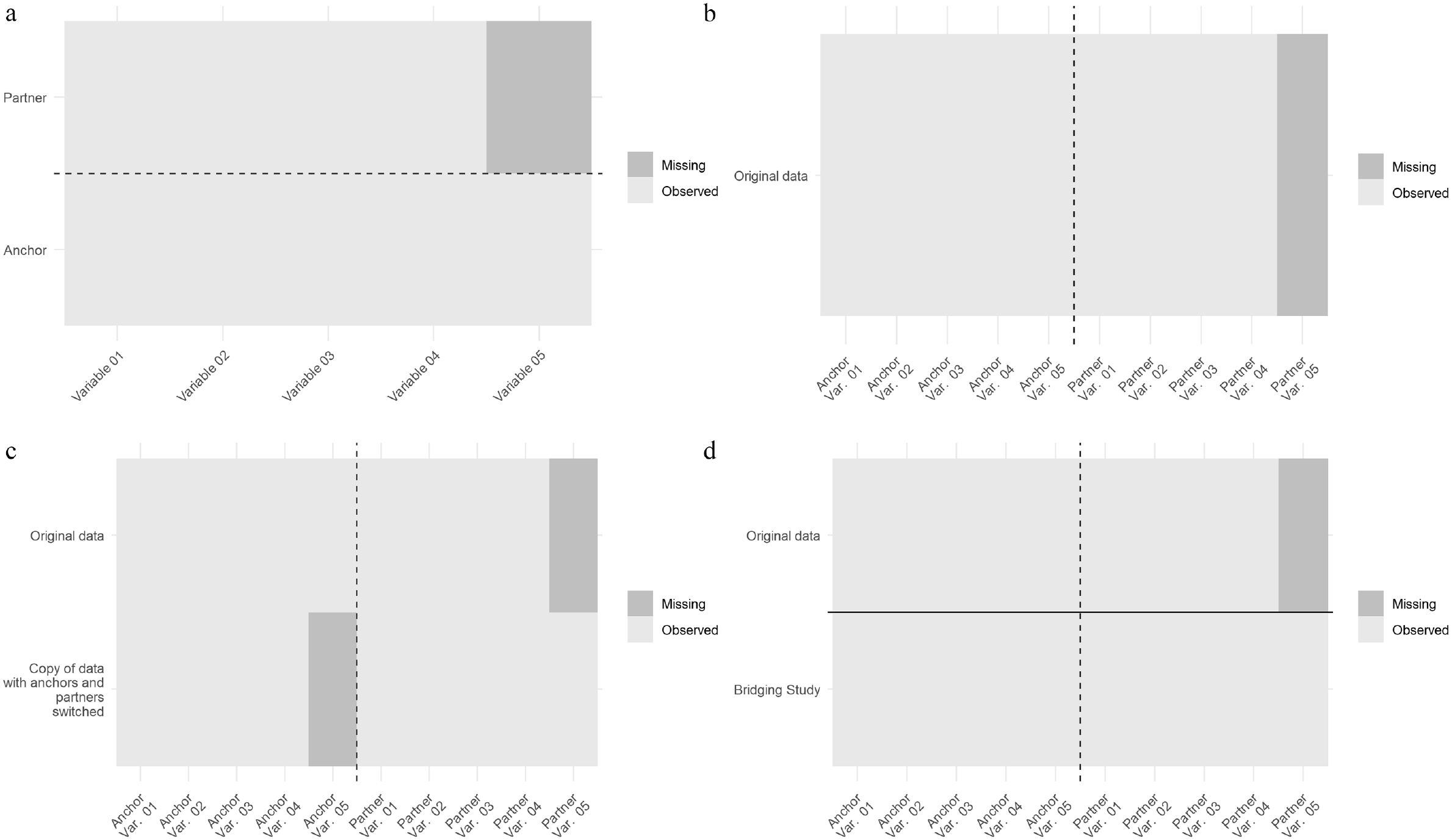
Data format for different imputation approaches: (a) anchor and partner data in long format, (b) anchor and partner data in wide format, (c) anchor and partner data in pairwise format, and (d) anchor and partner data with a bridging study added.
Imputing in wide format with one row for each relationship, that is, the format required for the target analysis (Figure 2b), is not possible with standard FCS procedures. Given that we do not have any observations in the systematically missing partner variable, the univariate imputation model cannot be estimated. A possibility would be to first transform the data into the pairwise format (Figure 2c). The pairwise format is well known in family research because the popular actor-partner interdependence models require this data structure (Kenny, Kashy, and Cook 2006; Kenny and la Voie 1985; Ledermann and Kenny 2012).
Actor-partner interdependence models measure bidirectional effects in interpersonal relationships. To transform the data set from the wide format to the pairwise format, we create a copy of the original data set with anchor and partner allocation exchanged (see Figure 2c). After restructuring, “current life satisfaction of partner” is filled, and “current life satisfaction of anchor” is empty for the copied data set. This allows us to impute the missing partner life satisfaction conditional on all other anchor and partner variables with a standard FCS procedure. However, while imputing, we still implicitly assume the partial correlation between anchor’s and partner’s life satisfaction given all other anchor and partner variables to be zero, because both variables are never observed together (see Figure 2c). Both imputation approaches, MI in long (2.) or pairwise format (3.), are thus built on the assumption of conditional independence. Although the two imputation approaches are relatively easy to implement, we will see whether this strong assumption holds in real-world settings.
If we do not wish to assume conditional independence but instead suspect a dependence between the two variables, we need to make reasonable assumptions about the strength of dependence, that is, the partial correlation. External information from a “bridging study” allows us to make such assumptions on the (conditional) dependence between the anchor and the (systematically missing) partner variable. There are two ways to use the information on anchor and partner respondents from bridging studies.
As a first possibility, we can append the bridging study to the original data set after the ex post survey harmonization (see Figure 2d). This allows estimation of the relationship between anchor and partner variables from the additional data set and, therefore, reflects the chosen assumptions (van Buuren 2017). In principle, one could retain the bridging studies and run the analyses on the pooled data. In our case, we use the additional data from pairfam and SHARE only for the imputation and exclude it from the analyses. Even though pairfam and SHARE are only used as a bridging study and not for a “complete” survey harmonization project, careful data preparation and harmonization is still necessary.
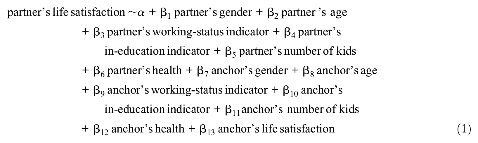
A second possibility is to specify the partial correlation between the observed anchor variable and the unobserved, systematically missing partner variable in the imputation model. We can obtain this parameter by estimating a regression of the variable systematically missing on the other variables (especially the corresponding anchor variable) in the bridging study and use estimated parameters in the imputation model. This might be advantageous if an ideal bridging study, which is (almost) identical to the main study is not available. This approach might be particularly interesting if the systematically missing partner variable constitutes an unobserved confounder, where we vary plausible (partial) correlations between anchor and partner to assess the robustness of the analyses (Frank 2000; Frank et al. 2023; Resche-Rigon et al. 2013). For example, partner’s life satisfaction can confound the relationship between anchor’s life satisfaction (exposure) and anchor’s mental health (outcome). Partner’s life satisfaction directly influences anchor’s life satisfaction, as a highly satisfied partner can contribute to a positive and supportive relationship, enhancing the anchor’s overall life satisfaction. Simultaneously, partner’s life satisfaction can affect anchor’s mental health, as a supportive and satisfied partner provides emotional and psychological support, improving the anchor’s mental health. Therefore, failing to account for partner’s life satisfaction could bias the estimated effect of anchor’s life satisfaction on their mental health.
We use different artificially created and real-world bridging studies to exemplify possible pitfalls and consequences of their usage. We first present a benchmark, that is, an ideal bridging study. We only include such a bridging study (“04. MI with an ideal bridging study”) to demonstrate a benchmark that other more realistic bridging studies will have to measure up to. Our ideal bridging study consists of a new set of 1,000 drawn observations from the original GSOEP panel with replacement. Measurements, target populations, and sampling are the same for the original target data set with systematically missing data. However, real-world bridging studies will often deviate from the original data set, for example, in the variables included, the measurements used, or other characteristics of a study, such as the mode, the year in which the survey was conducted, or the sampling and population.
Naturally, we are interested in the possible information gains not only under ideal conditions but also under real-world conditions. We explore this topic in the simulation and in a more general exploration of study heterogeneity. For both bridging studies, we evaluate two approaches:
Appending the additional bridging study to the original data set and then imputing the systematically missing data (“05. MI with SHARE added” and “07. MI with pairfam added”).
Separately estimating the parameters for the imputation model of the systematically missing variable and then using the obtained estimates to impute the values for the systematically missing variable (“06. MI with SHARE parameters” and “08. MI with pairfam parameters”). We follow the same steps as in regular imputation by the normal model as defined by Rubin (1987), except we use the data from the bridging study to estimate all parameters for the imputation model of the systematically missing variable. Apart from that, we follow the same steps as in the regular mice.impute.norm function.
We use the linear regression imputation approach for the partner’s life satisfaction with otherwise standard mice options. This leads to the following imputation model for the partner’s life satisfaction when using only sociodemographic variables:
Data and Simulation
Data Sets: GSOEP, SHARE, and pairfam
We demonstrate the consequences of different possible imputation approaches with data from the GSOEP (Goebel et al. 2019) and, as additional bridging studies, pairfam (Brüderl et al. 2017) and the German substudy of SHARE (Börsch-Supan 2020; Börsch-Supan et al. 2013). All three studies are longitudinal multiactor surveys and include self-reported information from the partner respondents; they collect similar data and provide information on cohabiting couples in Germany around 2013. Although the studies are longitudinal, we use their data purely as cross-sectional, that is, one wave from each survey. There is substantial overlap regarding several aspects of the study design, which is why we chose pairfam and SHARE as bridging studies, but the three studies have significant differences. In the simulation, we examine how these similarities and differences allow or prevent their use as bridging studies.
The GSOEP is a longitudinal household survey in Germany. We use data from the wave “bd” (2013). We restricted the data set to persons cohabiting with their partners, which encompasses 5,584 relationships. Variables include information on household composition, employment, occupation, health, and satisfaction indicators. Sociodemographic variables, psychological factors, and life satisfaction were observed for anchors and their partners. To evaluate the different imputation approaches, we delete the information on partners’ life satisfaction, thus intentionally creating systematically missing partner information.
SHARE (Börsch-Supan et al. 2013) surveys about 140,000 individuals aged 50 or older, covering 27 European countries and Israel. With the younger cohorts missing from SHARE, we already notice significant differences in comparison with GSOEP. We used data from the fifth wave of the survey, as it was conducted the same year as the GSOEP, wave “bd” (2013). We selected a subsample as a bridging study to increase the similarity between the samples: we selected only persons in Germany living together with their partners. The resulting SHARE bridging study then encompasses 1,920 relationships.
pairfam (Brüderl et al. 2017) collects data on anchor respondents and their partners (as well as other family members). We use data from the second wave of the pairfam panel, conducted around the same time (2011) as the selected GSOEP and SHARE waves: we have 2,192 cohabiting partnerships for which both anchor and partner responded to the survey. By its own description, pairfam is a “multidisciplinary, longitudinal study for researching partnership and family dynamics in Germany.” This data set has rich information on both anchors and partners; it consists of a nationwide random sample of about 12,000 persons from three birth cohorts (1971–1973, 1981–1983, 1991–1993) and their partners, parents, and children.
The three surveys thus differ to some extent with regard to population and sampling. However, surveys may also differ with regard to measurements. In our case, for instance, measurement of the Big Five personality traits differs between the GSOEP and pairfam. The item formulations, the number of items per dimension, and the scales (7 point vs. 5 point) differ. Therefore, before a bridging study can be used, the measures in the original and bridging study have to be harmonized. Here, we harmonized the GSOEP Big Five variables by shrinking them to a 5-point scale (Singh 2020). We also had to harmonize the variables for anchor’s and partner’s sex, age, health status in the past four weeks, indicators for being employed and being in education, and the number of biological children. The variable life satisfaction (systematically missing for partners) was measured in all surveys on an 11-point scale with the same alignment and the same question text. For the mapping of all variables used as predictors to a common scale, see Appendix Table A1.
Simulation Conditions
For each simulation run, we randomly select 1,000 observations with replacement from the GSOEP cohabiting relationships from the survey year 2013. Life satisfaction for the partner respondent is deleted before testing all MI approaches. We use all available data for the bridging studies, that is, data from 1,920 relationships from SHARE and 2,192 relationships from pairfam. We use 1,000 repetitions to compare all approaches.
We start by examining estimates of the correlation coefficient between anchor’s and partner’s life satisfaction to get an impression of the amount of dependence that can be recovered with simple MI approaches on the basis of the assumption of conditional independence (long format). We compare point estimates and standard errors throughout all conditions, that is, (2.) long format, (3.) pairwise format, (4.) ideal bridging study, (5.) SHARE bridging study, (6.) SHARE parameters, (7.) pairfam bridging study, and (8.) pairfam parameters.
Our second target analysis is a regression of anchor’s life satisfaction on partner’s life satisfaction, as well as sociodemographic variables and the Big Five personality traits for the anchors and partners. Again, we compare the performance of the different conditions in recovering the true estimate. In the target analysis, the information on anchor and partners is not used in long format (where all anchors and partners are in separate rows, see Figure 2a), but in wide format, that is, there is one row for each relationship with anchor and partner information in separate variables (see Figure 2b).
For all simulation runs and methods tested, every missing value is imputed five times (m = 5), and the number of iterations is set to 10. We checked convergence plots for every method and found no problems. We then use standard analysis for each of the
Results
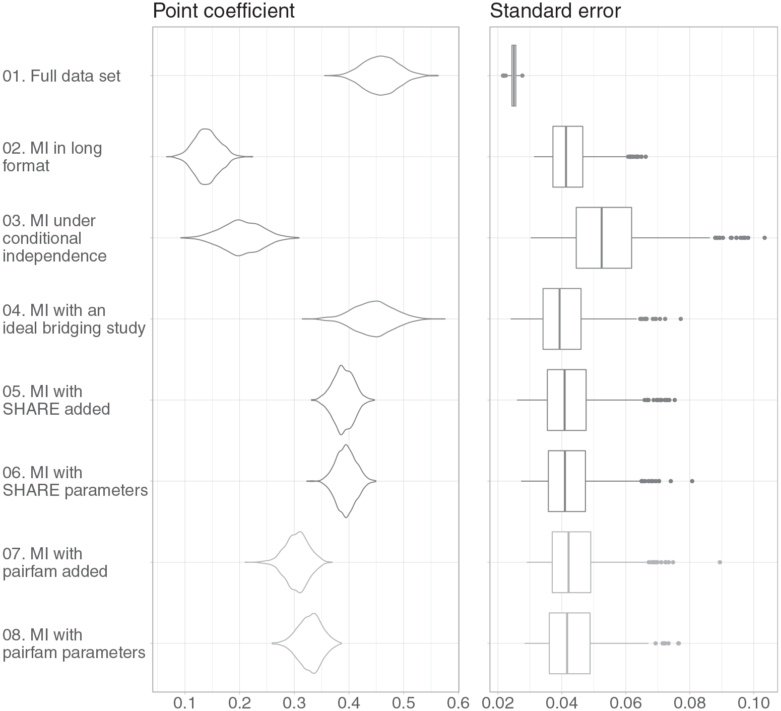
We first present the results for the estimates of the correlation between anchor’s and partner’s life satisfaction and, subsequently, the estimates of the regression coefficients. We examine point estimates and standard errors. Point estimates are presented in violin plots (Hintze and Nelson 1998), a visualization technique developed from boxplot and kernel density plots showing the distribution of data across several levels of a categorical variable. This allows us to compare these distributions easily. Standard errors are presented as boxplots.
Correlation Coefficient Results
We first look at the estimated raw correlation coefficients between the anchor respondent and the partner respondent’s current life satisfaction. We compare the results after MI in long format with the results from the full data sets (before artificial deletion of the partner’s life satisfaction values). After MI in long format (2.), the estimated point coefficients for the correlation between the anchor’s and partner’s current life satisfaction are strongly biased toward zero, that is, a mean value for the correlation coefficient of .141 versus .460 for the full data set (see also Figure 3). This result can be explained easily, considering that under MI in long format (see the data format in Figure 2a), a possible dependency between anchor’s and partner’s life satisfaction cannot be taken into account properly and the partial correlation is implicitly assumed to be zero.
Anchor’s current life satisfaction and partner’s current life satisfaction.
The bias toward zero for the estimated correlation coefficient is also prevalent after MI in pairwise format (3., correlation coefficient mean value .284). Although information from both anchors and partners are now included in the imputation model with the data in pairwise format, the estimates are still biased toward zero. This indicates that the implicit assumption of conditional independence is not appropriate. Apparently, there is an association between anchor’s and partner’s life satisfaction that cannot be attributed to the (dyadic) associations in the other variables.
To get an idea of what can principally be achieved with a bridging study, we include an ideal bridging study with a large number of observations and no differences in measurements, variables, sampling, or underlying population. Not surprisingly, the point estimates are unbiased after MI with a bridging study consisting of another sample of 1,000 observations from the GSOEP (4.). Standard errors are higher than for the full data set because of the loss of information from missing data (Carpenter and Kenward 2013:54).
We now turn to real-world bridging studies (5. to 8.). Although we still underestimate the correlation coefficients after MI when using the information in either pairfam or SHARE, the estimates are less biased than under the assumption of conditional independence (mean values for the correlation coefficient estimates range between .394 and .306).
Finally, we do not append the bridging studies, as in conditions 5. and 7., but input the parameters—the partial correlation between the anchors’ and their partners’ life satisfaction—obtained through the bridging studies directly into the imputation models. The differences between appending the bridging studies pairfam and SHARE to the original data set (5. and 7.) and using the sampling distribution of the estimates from the bridging studies for the imputation model (6. and 8.) are minor.
Regression Coefficient Results
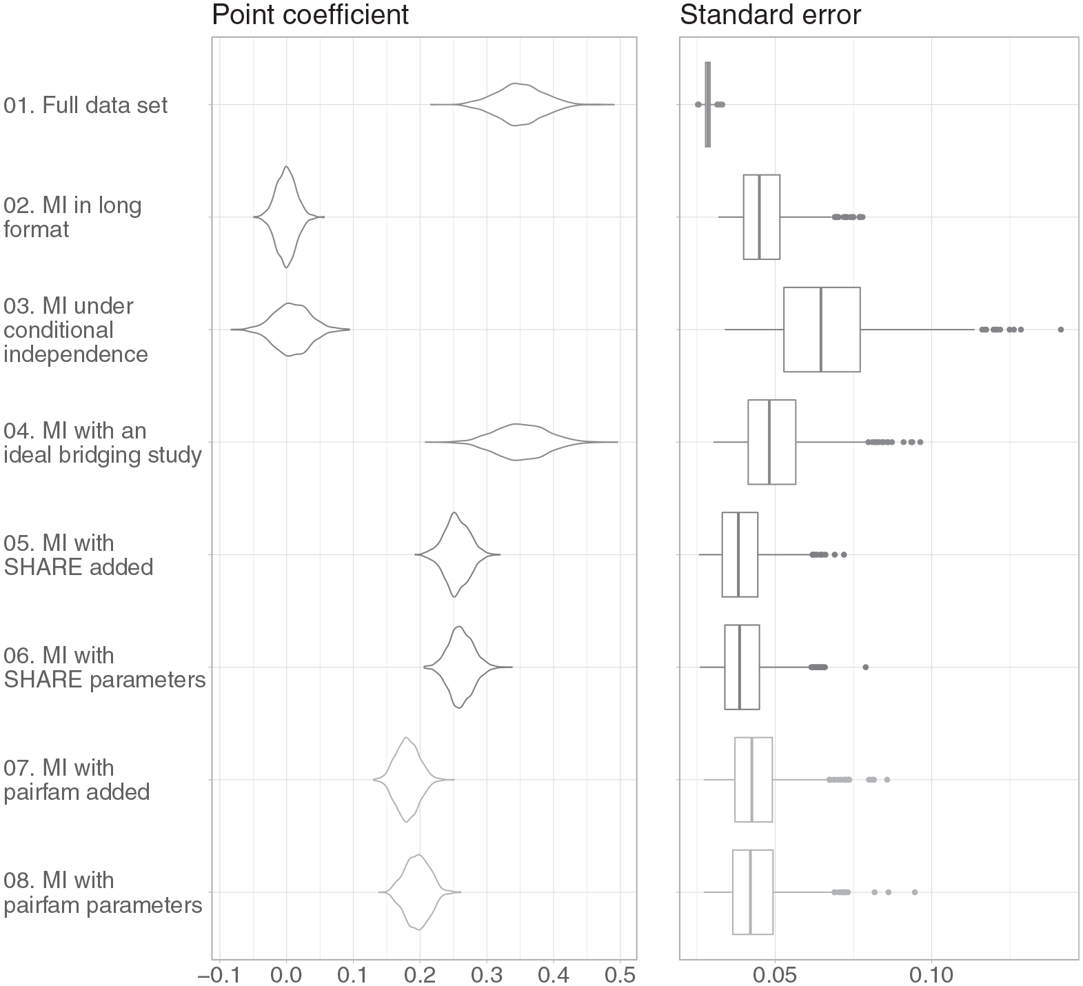
In this section, we focus on the partial correlation between the anchor’s and partner’s current life satisfaction. We conducted two simulations, the main one in which the variables in the imputation model match the variables in the analysis model (excluding Big Five personality traits variables), and one in which the imputation model is richer than the analysis model (including the Big Five personality variables as auxiliary variables). Auxiliary variables are used for imputation for two reasons: if the auxiliary variables are good predictors of missing values, they will help recover missing information. Plus, if they are good predictors of the missingness, they may even correct bias (Carpenter and Kenward 2013). We present the results from the first simulation in Figure 4, where the variables in the imputation model and the analysis model are the same. The results of the second simulation, in which the imputation model has fewer variables than the analysis model, are included in the Appendix.
Main simulation.
Looking at the results from the main simulation, we see that the density of the estimated point coefficients after both MI in long format (2.) and MI in pairwise format (3.) are centered around zero and, therefore, heavily biased (Figure 4). When we impute the data in a long format, we neglect the fact that the anchor and partner variables are correlated with each other. Similarly, when we assume conditional independence between an anchor and partner variable pair during imputation with the data in a pairwise format, our results show this independence after imputation.
Regarding bridging studies, the ideal bridging study performs well (4. in Figure 4) in recovering the true association. However, as in the previous section, the standard errors are larger. If we use more realistic bridging studies, either with the data added or with the parameters used in the imputation model, the results are still biased toward zero. However, the use of either bridging study (5. and 6. vs. 7. and 8.) substantially reduces bias compared with imputation in the long format (2.) or in the pairwise format (3.). Again, we do not observe notable differences between adding a bridging study and using parameters that were estimated separately from the bridging study before imputing.
Summarizing the results of the main simulation, we find that the assumption of conditional independence leads to nonoptimal results. As we suspected, the assumption of conditional independence is not appropriate (mean of estimated regression coefficient is .008 instead of .349 for the full data set). Using bridging studies (or their parameters) leads to better results in regard to lower bias (mean results range from .181 to .261). However, the two bridging studies perform differently. These differences could result from differences in target population between the original data set and the respective bridging study. We take a closer look at what can be expected in terms of the magnitude of study heterogeneity in the next section.
Before turning to study heterogeneity, we briefly mention the simulation results in the Appendix, in which we did not include the Big Five personality traits in the analysis model. We still include them as auxiliary variables (Enders 2017) in the imputation model when possible (so for all approaches except for SHARE, because they were not available in the respective wave). Our imputation model for 02. to 04. and 07. and 08. is thus richer than the analysis model.
The results for the second simulation (Figure A1) strongly resemble the results of the main simulation (Figure 4). The point estimates after MI in long format and MI in pairwise format are again biased downward in the second simulation (mean of estimates .036 and .063 instead of .377 for the full model). We observe a partial correlation between anchor and partner only because the analysis model does not include all variables from the imputation model. These additional or auxiliary variables are correlated with anchor’s and partner’s current life satisfaction, and as a result, the regression coefficient of partner’s life satisfaction is not zero. Similar to the main simulation, MI with pairfam and now also SHARE leads to underestimation of the point coefficients (mean of estimates ranging from .193 to .278). Again, the bias is not as substantial as after MI in pairwise format or after MI in long format.
From these simulations, we can draw three important conclusions. First, the assumption of conditional independence is not suited for the imputation of partner variables in our case because it leads to a substantial underestimation of the (partial) correlation between anchor and partner variables. Second, the use of bridging studies improves the imputation. The closer the bridging study is to the original study, the better the imputation. Ideal bridging studies have a sufficiently high number of observations and are as similar as possible to the original study. Third, specifying parameters for the partial correlation between anchor and spouse—in our case obtained by estimating multivariate regression models with the bridging studies—works just as well as using the bridging studies themselves. However, this approach is limited to cases in which the set of variables in the imputation model matches those in the analysis model or the partial correlation is not dependent on missing variables.
Study Heterogeneity
The previous results show that the different bridging studies perform differently. The ideal bridging study recovers the true (partial) association between anchor’s and respondent’s life satisfaction. This is not surprising, considering that the original study and bridging study do not differ with respect to (1) underlying population, (2) sampling, (3) interview mode, or (4) measurements (Dong et al. 2014; Roberts and Binder 2009). The other studies, SHARE and pairfam, as well as using their parameters, perform considerably better than imputing under the assumption of (conditional) independence, but differ in their respective performance. One starting point for understanding these differences is heterogeneity in studies.
When choosing a bridging study, meta-analyses or systematic reviews can be the first source to check whether study heterogeneity is likely to affect the imputation model and consequently the estimates of interest. A second possibility is to empirically assess differences between the original study and potential bridging studies. To exemplify this, we first present descriptive statistics for the study variables from the three surveys as boxplots (see Figure 5). Most of the point and variance estimates do not differ sharply between the surveys, except for the age variable. This is due to the sampling schemes for the three surveys, which all differ in that regard. GSOEP surveys the general population age 16 and older, SHARE only includes anchors age 50 or older, and pairfam surveys only anchors from the birth cohorts 1971–1973, 1981–1983, and 1991–1993. AppendixTables A2 to A4 present descriptive statistics for the variables in the three studies. These statistics also show that the studies differ with regard to age and age-related characteristics, for instance, labor force status and number of children, with GSOEP and SHARE being more similar than GSOEP and pairfam.
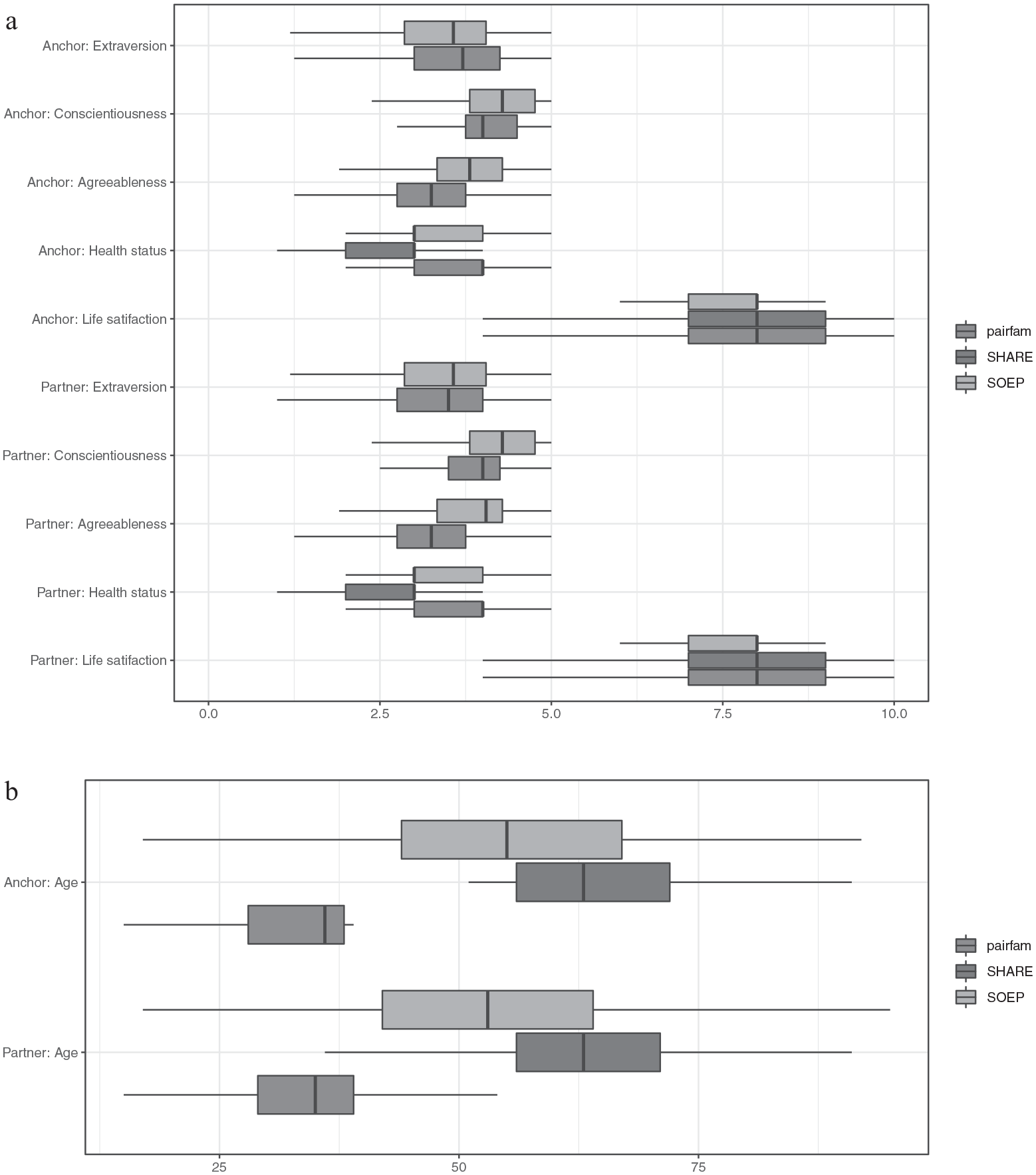
Box plots of selected variables. (a) Selected Big Five traits and life satisfaction for anchor and partner respondents. (b) Age for anchor and partner respondents.
This is also a warning sign that relationships between variables that include age or for which age is a moderator may be nontransferable between the three surveys. At the same time, differences in univariate distributions do not necessarily mean that relationships between variables are also affected by heterogeneity between surveys. Thus, we recommend checking differences in the magnitude and sign of variables that are available for all surveys to check whether differences in the study design might affect the relationship between different variables.
To look at the differences in relationships between variables for the three studies, we estimated a series of regressions for the relationship between the different anchor and partner variables in the pairfam, GSOEP, and SHARE data sets (see Figure 6). We restricted all data sets to anchors cohabiting with their partners and for whom data on partners is available.
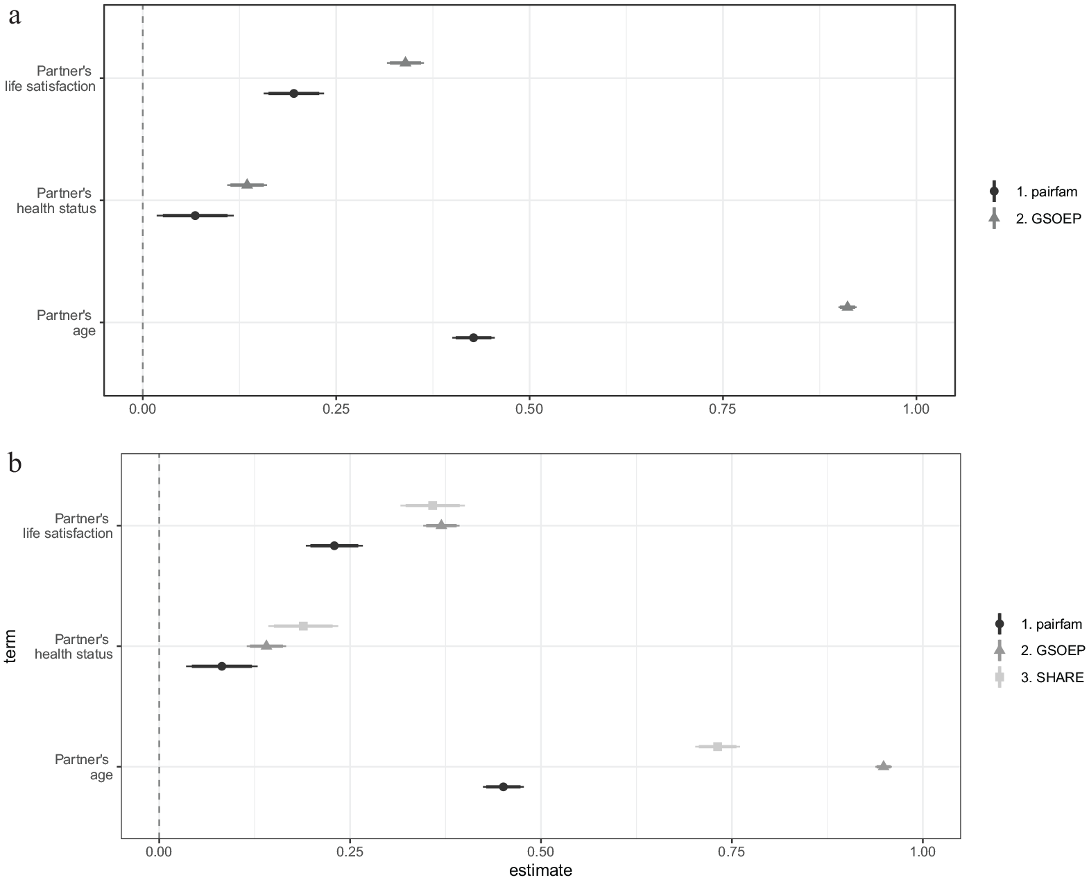
Point estimates of partner variables. (a) Sociodemographic and Big Five variables for both anchor and partner are included as predictors. (b) Sociodemographic variables for anchor and partner are included as predictors.
For every anchor variable as the outcome variable, that is, for every estimate displayed, we estimated a separate model. The estimated regression coefficient for every partner variable (always with the corresponding anchor variable as the dependent variable) is displayed. For Figure 6a, all other sociodemographic and Big Five personality traits variables for both anchor and partner are always included as predictors, that is, are conditioned on. For Figure 6b, all other sociodemographic variables for both anchor and partner are included as predictors. First, Figure 6 shows that the point estimates in the three surveys are all the same sign and, with the exception of age, of similar magnitude. Second, the point estimates from the GSOEP and SHARE are closer than those from pairfam. This fits with the previous finding that using SHARE as a bridging study leads to lower bias in the estimates than using the GSOEP (see Figures 3, 4, and A1). Third, this appears to be due to higher similarity between anchors and partners in GSOEP and SHARE compared with pairfam.
Investigating study heterogeneity appears indispensable if one intends to use a bridging study to impute systematically missing partner variables. However, this does not give an accurate assessment of whether a study is similar enough to be used as a bridging study. It can only be used as a plausibility check to assess whether the auxiliary study is suitable at all. In practical application, it is highly unlikely that an ideal bridging study will be available. On the contrary, it is likely that the available bridging studies differ with respect to one or more characteristics concerning population, sampling, mode, or measurement. Instead of using only the bridging study for MI, it seems more advisable to specify a range of plausible values for the (partial) correlation. However, what counts as a range of plausible values depends on the nature of the missing characteristic and cannot be established a priori.
Discussion
In this article we explore if and how MI can be used in multiactor surveys when there is systematically missing data for specific types of respondents, such as partner respondents. Similar problems have been addressed with MI techniques, such as missing confounders in meta-analyses of IPD (Resche-Rigon et al. 2013), missing variables in split-questionnaire designs (Rässler 2003), bridging old and new measures in repeated surveys (Parker et al. 2004; Schenker and Raghunathan 2007), and combining probability and nonprobability samples (Kim et al. 2021). We contribute to the literature by investigating the feasibility of the bridging study approach in the context of multiactor studies, using information about the relationship between variables from an additional data source, a bridging study.
A particular challenge in multiactor studies is the interdependence between anchors and secondary respondents, such as homogamy or heterogamy in partnerships (Kalmijn 1998). We thus also present a novel approach where we do not use a bridging study but instead incorporate auxiliary information about the interdependence between anchor and partner directly into the imputation model. In our motivational example, we used the GSOEP, in which the variables of interest, partners’ and anchors’ life satisfaction, were initially observed. By deleting all information on partners’ life satisfaction, we created systematically missing data in partner variables for a simulation to assess results of the imputation approaches. We examined different MI approaches to impute the missing information for partners’ life satisfaction, with and without use of bridging studies (Parker et al. 2004; Schenker and Raghunathan 2007) or auxiliary information (Moretti and Shlomo 2023).
We draw five important conclusions from our study. First, the two approaches that do not use bridging studies or auxiliary information (and thus do not take the conditional dependence between anchor and partner properly into account) performed poorly. Imputing data in long format and imputing the systematically missing partner data using a pairwise data format (observation units are relationships and anchor’s and partner’s information are combined in one row) both lead to severely biased estimates. The inappropriateness of assuming conditional independence has also been stated in other contexts related to systematically missing data, such as record linkage (Thibaudeau 1993; Winkler 1989). The general recommendation is to incorporate more suitable assumptions about the conditional dependence between the two variables (Bosch and Gaffert 2017). We chose to do so through bridging studies, which leads to the next set of results.
Second, an ideal bridging study is similar to the original study regarding (1) underlying population, (2) sampling, (3) interview mode, and (4) measurements. This is often (almost) achieved in the case of panel studies, because one can take another wave where all variables were observed, but it is not restricted to panel studies. In our case, the “ideal” constituted another subsample randomly drawn from the GSOEP data that we used for the simulation. Because this represents an ideal situation, we also included a more realistic situation.
Third, we additionally chose different studies to serve as bridging studies: SHARE (Börsch-Supan 2020; Börsch-Supan et al. 2013) and pairfam (Brüderl et al. 2017). We found that the results using bridging studies are much better in terms of bias than the two approaches based on (conditional) independence assumptions. We do want to note that using bridging studies to impute systematically missing variables is based on the assumption that study heterogeneity is not too great to hinder the transfer of relationships between studies.
Fourth, it is important to find a suitable bridging study. A good bridging study should have a sufficient sample size and be similar in population and design to the sample with systematically missing data. To mitigate potential differences, researchers can use methods from the survey harmonization literature. The literature on survey harmonization proposes different methods to adjust several samples that differ in sampling or weighting, for example, adjusting survey data with official statistics, such as census data or a register (Deville and Särndal 1992; Deville, Särndal, and Sautory 1993), calibration to align surveys from different sources (Guandalini and Tillé 2017), or optimal transport to combine data sets (Garès and Omer 2022; Guernec et al. 2022).
With regard to measurement methods, Singh (2022) pointed to three important dimensions that should be evaluated when comparing measurements: (1) Is the construct being measured the same by both instruments? (2) Are both instruments equally reliable in measuring the same construct? Raykov and Marcoulides (2011) demonstrated how to compare multi-item instruments regarding these questions. And (3), one should evaluate whether the units of measurement are similar for both instruments. Because this might be one of the most frequent deviations in measurement between surveys, Singh (2022) discussed two methods to harmonize such instruments: linear stretching, which we used here, and observed score equating. Additionally, the Dempster-Shafer theory can be applied to manage uncertainties in attribute values when integrating data from different sources (Lim, Srivastava, and Shekhar 1994). There is, however, one important exception where suitable bridging studies are available—this holds for both multiactor and single respondent studies—repeated cross-sections. In this case, prior waves can be used, as they usually do not differ with regard to underlying population, sampling, interview mode, or measurements (Dong et al. 2014; Roberts and Binder 2009).
One might also extend the proposed idea to longitudinal multiactor studies if, for instance, the partners are interviewed at larger intervals than the anchors. In this case, prior waves could potentially be used to impute the systematically missing information in the current wave, given that the information was recorded for anchor and partner in the prior wave. However, this would need to be tested empirically, taking into account the special features of longitudinal imputation (Young and Johnson 2015). Fifth, using auxiliary information about the conditional dependence and specifying this directly in the imputation model performs just as well as using an (ideal) bridging study. The differences between the two approaches were minor in our example. 5
In future research, it would be beneficial to compare not only the direct correlation between anchor and partner variables but also the effects of other variables in the multivariate model to further illustrate the effect of the missing partner variable as a confounder. Future research could also investigate the feasibility of the approaches in other dyadic relationships, for example, parent-child or employer-employee relationships. However, these relationships often exhibit systematic differences that are not typically present in anchor-partner relationships. The limitations of imputation approaches that do not account for conditional dependence and the need for bridging studies or auxiliary information becomes even more apparent in these cases because of these inherent differences.
Footnotes
Appendix
Overview of Harmonized Data Sets and Mapping of Values to the Variables Used for Analysis.
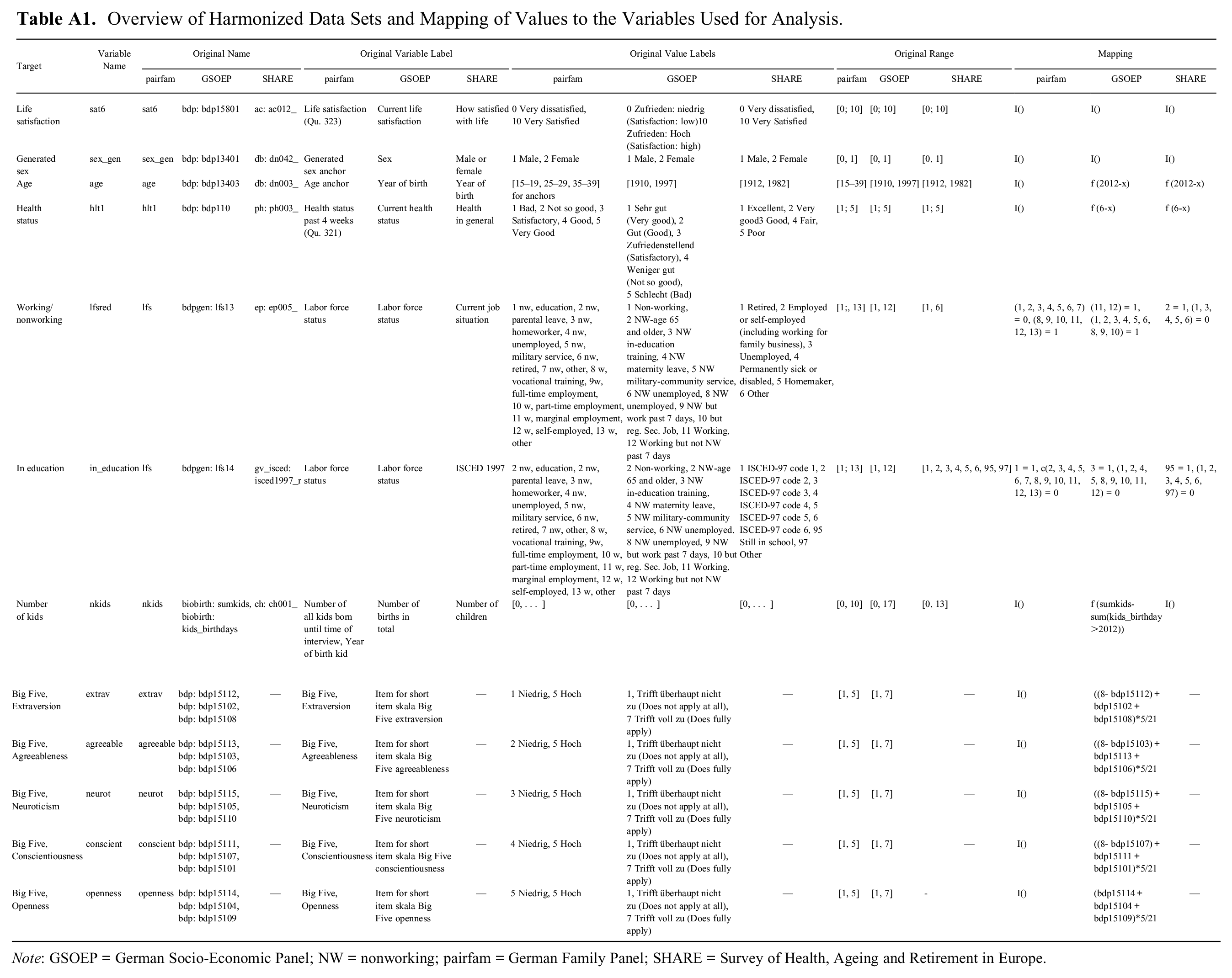
| Target | Variable Name | Original Name | Original Variable Label | Original Value Labels | Original Range | Mapping | ||||||||||
|---|---|---|---|---|---|---|---|---|---|---|---|---|---|---|---|---|
| pairfam | GSOEP | SHARE | pairfam | GSOEP | SHARE | pairfam | GSOEP | SHARE | pairfam | GSOEP | SHARE | pairfam | GSOEP | SHARE | ||
| Life satisfaction | sat6 | sat6 | bdp: bdp15801 | ac: ac012_ | Life satisfaction (Qu. 323) | Current life satisfaction | How satisfied with life | 0 Very dissatisfied, 10 Very Satisfied | 0 Zufrieden: niedrig (Satisfaction: low)10 Zufrieden: Hoch (Satisfaction: high) | 0 Very dissatisfied, 10 Very Satisfied | [0; 10] | [0; 10] | [0; 10] | I() | I() | I() |
| Generated sex | sex_gen | sex_gen | bdp: bdp13401 | db: dn042_ | Generated sex anchor | Sex | Male or female | 1 Male, 2 Female | 1 Male, 2 Female | 1 Male, 2 Female | [0, 1] | [0, 1] | [0, 1] | I() | I() | I() |
| Age | age | age | bdp: bdp13403 | db: dn003_ | Age anchor | Year of birth | Year of birth | [15–19, 25–29, 35–39] for anchors | [1910, 1997] | [1912, 1982] | [15–39] | [1910, 1997] | [1912, 1982] | I() | f (2012-x) | f (2012-x) |
| Health status | hlt1 | hlt1 | bdp: bdp110 | ph: ph003_ | Health status past 4 weeks (Qu. 321) | Current health status | Health in general | 1 Bad, 2 Not so good, 3 Satisfactory, 4 Good, 5 Very Good | 1 Sehr gut (Very good), 2 Gut (Good), 3 Zufriedenstellend (Satisfactory), 4 Weniger gut (Not so good), 5 Schlecht (Bad) | 1 Excellent, 2 Very good3 Good, 4 Fair, 5 Poor | [1; 5] | [1; 5] | [1; 5] | I() | f (6-x) | f (6-x) |
| Working/nonworking | lfsred | lfs | bdpgen: lfs13 | ep: ep005_ | Labor force status | Labor force status | Current job situation | 1 nw, education, 2 nw, parental leave, 3 nw, homeworker, 4 nw, unemployed, 5 nw, military service, 6 nw, retired, 7 nw, other, 8 w, vocational training, 9w, full-time employment, 10 w, part-time employment, 11 w, marginal employment, 12 w, self-employed, 13 w, other | 1 Non-working, 2 NW-age 65 and older, 3 NW in-education training, 4 NW maternity leave, 5 NW military-community service, 6 NW unemployed, 8 NW unemployed, 9 NW but work past 7 days, 10 but reg. Sec. Job, 11 Working, 12 Working but not NW past 7 days | 1 Retired, 2 Employed or self-employed (including working for family business), 3 Unemployed, 4 Permanently sick or disabled, 5 Homemaker, 6 Other | [1;, 13] | [1, 12] | [1, 6] | (1, 2, 3, 4, 5, 6, 7) = 0, (8, 9, 10, 11, 12, 13) = 1 | (11, 12) = 1, (1, 2, 3, 4, 5, 6, 8, 9, 10) = 1 | 2 = 1, (1, 3, 4, 5, 6) = 0 |
| In education | in_education | lfs | bdpgen: lfs14 | gv_isced: isced1997_r | Labor force status | Labor force status | ISCED 1997 | 2 nw, education, 2 nw, parental leave, 3 nw, homeworker, 4 nw, unemployed, 5 nw, military service, 6 nw, retired, 7 nw, other, 8 w, vocational training, 9w, full-time employment, 10 w, part-time employment, 11 w, marginal employment, 12 w, self-employed, 13 w, other | 2 Non-working, 2 NW-age 65 and older, 3 NW in-education training, 4 NW maternity leave, 5 NW military-community service, 6 NW unemployed, 8 NW unemployed, 9 NW but work past 7 days, 10 but reg. Sec. Job, 11 Working, 12 Working but not NW past 7 days | 1 ISCED-97 code 1, 2 ISCED-97 code 2, 3 ISCED-97 code 3, 4 ISCED-97 code 4, 5 ISCED-97 code 5, 6 ISCED-97 code 6, 95 Still in school, 97 Other | [1; 13] | [1, 12] | [1, 2, 3, 4, 5, 6, 95, 97] | 1 = 1, c(2, 3, 4, 5, 6, 7, 8, 9, 10, 11, 12, 13) = 0 | 3 = 1, (1, 2, 4, 5, 8, 9, 10, 11, 12) = 0 | 95 = 1, (1, 2, 3, 4, 5, 6, 97) = 0 |
| Number of kids | nkids | nkids | biobirth: sumkids, biobirth: kids_birthdays | ch: ch001_ | Number of all kids born until time of interview, Year of birth kid | Number of births in total | Number of children | [0, …] | [0, …] | [0, …] | [0, 10] | [0, 17] | [0, 13] | I() | f (sumkids-sum(kids_birthday >2012)) | I() |
| Big Five, Extraversion | extrav | extrav | bdp: bdp15112, bdp: bdp15102, bdp: bdp15108 | — | Big Five, Extraversion | Item for short item skala Big Five extraversion | — | 1 Niedrig, 5 Hoch | 1, Trifft überhaupt nicht zu (Does not apply at all), 7 Trifft voll zu (Does fully apply) | — | [1, 5] | [1, 7] | — | I() | ((8- bdp15112)+ bdp15102+ bdp15108)*5/21 | — |
| Big Five, Agreeableness | agreeable | agreeable | bdp: bdp15113, bdp: bdp15103, bdp: bdp15106 | — | Big Five, Agreeableness | Item for short item skala Big Five agreeableness | — | 2 Niedrig, 5 Hoch | 1, Trifft überhaupt nicht zu (Does not apply at all), 7 Trifft voll zu (Does fully apply) | — | [1, 5] | [1, 7] | — | I() | ((8- bdp15103)+ bdp15113+ bdp15106)*5/21 | — |
| Big Five, Neuroticism | neurot | neurot | bdp: bdp15115, bdp: bdp15105, bdp: bdp15110 | — | Big Five, Neuroticism | Item for short item skala Big Five neuroticism | — | 3 Niedrig, 5 Hoch | 1, Trifft überhaupt nicht zu (Does not apply at all), 7 Trifft voll zu (Does fully apply) | — | [1, 5] | [1, 7] | — | I() | ((8- bdp15115)+ bdp15105+ bdp15110)*5/21 | — |
| Big Five, Conscientiousness | conscient | conscient | bdp: bdp15111, bdp: bdp15107, bdp: bdp15101 | — | Big Five, Conscientiousness | Item for short item skala Big Five conscientiousness | — | 4 Niedrig, 5 Hoch | 1, Trifft überhaupt nicht zu (Does not apply at all), 7 Trifft voll zu (Does fully apply) | — | [1, 5] | [1, 7] | — | I() | ((8- bdp15107)+ bdp15111+ bdp15101)*5/21 | — |
| Big Five, Openness | openness | openness | bdp: bdp15114, bdp: bdp15104, bdp: bdp15109 | — | Big Five, Openness | Item for short item skala Big Five openness | — | 5 Niedrig, 5 Hoch | 1, Trifft überhaupt nicht zu (Does not apply at all), 7 Trifft voll zu (Does fully apply) | — | [1, 5] | [1, 7] | - | I() | (bdp15114+ bdp15104+ bdp15109)*5/21 | — |
Note: GSOEP = German Socio-Economic Panel; NW = nonworking; pairfam = German Family Panel; SHARE = Survey of Health, Ageing and Retirement in Europe.
Funding
The authors disclosed receipt of the following financial support for the research, authorship, and/or publication of this article: Funding for this research was provided by the Deutsche Forschungsgemeinschaft (DFG) under the projects “Bildungssysteme und migrationsspezifische Bildungsungleichheit” (DFG Project Number 430266278) and “Harmonisierung und Synthese von paarbiografischen Daten: Ein Modellprojekt zur Verknüpfung von Forschungsdaten aus verschiedenen Infrastrukturen” (DFG Project Number 316901171).