
Abstract
The flow of resources across nodes over time (e.g., migration, financial transfers, peer-to-peer interactions) is a common phenomenon in sociology. Standard statistical methods are inadequate to model such interdependent flows. We propose a hierarchical Dirichlet-multinomial regression model and a Bayesian estimation method. We apply the model to analyze 25,632,876 migration instances that took place between Turkey’s 81 provinces from 2009 to 2018. We then discuss the methodological and substantive implications of our results. Methodologically, we demonstrate the predictive advantage of our model compared to its most common alternative in migration research, the gravity model. We also discuss our model in the context of other approaches, mostly developed in the social networks literature. Substantively, we find that population, economic prosperity, the spatial and political distance between the origin and destination, the strength of the AKP (Justice and Development Party) in a province, and the network characteristics of the provinces are important predictors of migration, whereas the proportion of ethnic minority Kurds in a province has no positive association with in- and out-migration.
Keywords
Flows of items such as people, resources, and information across a finite number of units such as places, institutions, and individuals over time constitute a common type of data in sociology and the wider social sciences. Migration is one of the most frequent types of such flows; other examples include financial transfers between institutions or individuals, passengers through transportation systems, mobility tables, and the number of times participants trust or allocate a fixed resource to others during an experiment. Due to the highly interdependent nature of such situations, certain modeling problems arise (e.g., destinations “compete” over a fixed amount of flow) that are not straightforward to address with standard statistical models (Block, Stadtfeld, and Robins 2022).
Here we aim to contribute methodologically to the analysis of such dynamic flows. We frame our model within a migration context. Indeed, we developed our model with a motivation to analyze real-world migration data. Nevertheless, our model can be applied to other situations that similarly involve dynamic discrete flows across a finite number of units. One of the most widely used methods of analyzing migration flows is the gravity model (Barthélemy 2011; Expert et al. 2011; Karemera, Oguledo, and Davis 2000). In this model, the (logarithm) of the number of people migrating from
In this study, we propose a Dirichlet-multinomial model, which is an extension of a class of econometric discrete-choice models (Alamá-Sabater, Alguacil, and Bernat-Martí 2017; Guimaraes and Lindrooth 2007). Our model differs from existing choice models in the treatment of nonmigration. The existing models base their estimates conditional on migration taking place. We believe any inference about the causes of migration would be problematic if one ignores those who choose to not move: that is, observations for which the causes of migration might have been present but did not generate migration, or nonmigration counts. Ignoring nonmigration results in “selection on the dependent variable.” In our model, the probabilities of migration to the available destinations as well as the probability of not migrating are directly modeled as functions of the covariates. We further extend our model with random intercepts for provinces to account for the longitudinal nature of migration flows. We fit our model within the Bayesian framework via a Markov chain Monte Carlo (MCMC) algorithm.
A long array of models, developed mostly in the social networks literature, can also be applied to dynamic flows. These include stochastic actor-oriented models (Snijders 1996, 2001), dynamic network actor and other similar relational event models (Block, Stadtfeld, and Snijders 2019; Stadtfeld and Block 2017; Stadtfeld, Hollway, and Block 2017b), exponential random graph models (Lusher, Koskinen, and Robins 2013) and its various extensions and forms (Almquist and Butts 2014; Block et al. 2022; Desmarais and Cranmer 2012; Krivitsky and Butts 2017; Krivitsky and Handcock 2014; Westveld and Hoff 2011), and latent space and latent factor models (Hoff, Raftery, and Handcock 2002; Minhas, Hoff, and Ward 2019). Some of these models are theoretically flexible and very general but may be difficult to adapt to the specific case; others are computationally demanding. The application of some require significant programming. Nevertheless, these models offer a powerful way of dealing with relational data. We believe our approach provides a relatively straightforward and natural way to deal with dynamic flows while also offering computational simplicity and taking into account key features of the data. We discuss similarities and differences between our model and these network models in the “Related Methodology” section. We contribute to the methodological literature by enriching the methodological arsenal for dealing with dynamic flows.
This article also contributes to the migration literature. Prior work has identified various determinants of voluntary migration (Boyle, Halfacree, and Robinson 1998). These include characteristics of the origin and the destination, such as economic prospects (Borjas 1999; Levy 2010) and immigration legislation (Palmer and Pytlikova 2015), and characteristics of the origin-destination pair, such as linguistic, cultural, and physical distance (Expert et al. 2011; Levy 2010; Windzio 2018) between the origin and the destination. Migration can be international as well as intranational. Yet the migration literature is based mostly on international migration, and hence the dynamics of internal migration, particularly in non-Western countries, are understudied (Bell and Muhidin 2009; Kuhn 2015). The focus on international migration is understandable, given that it is highly consequential in shaping public opinion and politics (Chan et al. 2020; Gimpel and Schuknecht 2001). The scarcity of research on internal migration, however, is surprising. Internal migration may not be as economically advantageous for the migrant or as topical as international migration. However, it is far less costly and risky. Consequently, compared to international migration, much larger shares of populations are affected by internal migration, particularly in non-Western countries (Kuhn 2015). For example, according to the official statistics, in 2018, a total of 323,918 people emigrated abroad from Turkey, our study context, yet 3,057,606, nearly 10 times more, moved from one Turkish province to another. Internal migration is thus a strong determinant of local population structures, and it is important to understand its drivers.
We contribute to the migration literature by addressing this gap. Using a unique data set compiled from administrative, registry, and survey data, we analyze the dynamics of more than 25 million migration instances between the 81 provinces of Turkey from 2009 to 2018. Almost all empirical work on internal migration in Turkey, however scarce, has been conducted with data spanning until 2000 (Filiztekin and Gökhan 2008; Gedik 1997; Yazgi et al. 2014). The more recent work is descriptive and focuses on larger interregional migration (Akın and Dökmeci 2015). Over this period, Turkey went through a large economic, demographic, and political transformation (Aksoy and Billari 2018), which has affected migration (Çoban 2013). We thus do not know if these earlier insights into Turkey’s internal migration will apply to more recent migration patterns. Internal migration in Turkey is relevant for Europe, too. Turkey’s ascension to the European Union (EU) has stalled. One of the fears blocking expansion of the EU is large-scale immigration (Strasser 2008). Understanding the determinants of interprovince migration in Turkey will help predict the extent of potential migration from Turkey to Europe and its likely destinations within the EU, should Turkey ever be part of the EU (Filiztekin and Gökhan 2008).
A Model of Migration Flows
We now describe our model in a migration context. Note that our model can be applied to many other settings with minimal adjustment, for example, provinces can be replaced by individuals or institutions, and migration can be replaced by the number of financial transfers or interactions. In fact, in many of these alternative settings, one could directly proceed with modeling the Ht(i,j)s in the following. The migration case needs a slight adjustment, as we will describe, because the stock of people who could migrate but did not is dynamic due to changes in births and deaths.
Assume we have

for all
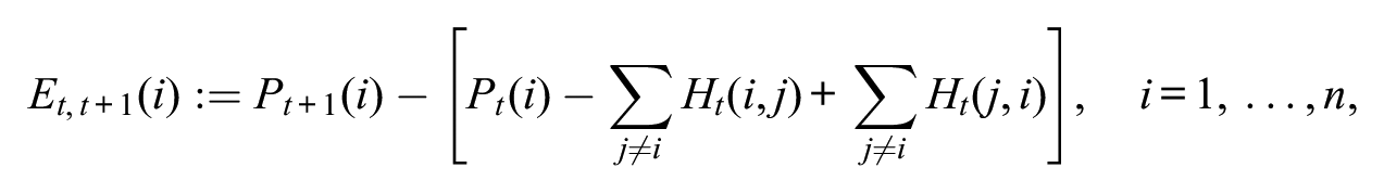
which is the net change in population for province
We consider this adjusted population to find the number of people who did not migrate from province

Therefore, given the assumptions, we can summarize the relation between the quantities
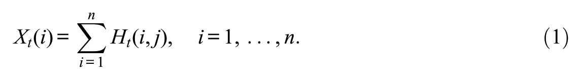
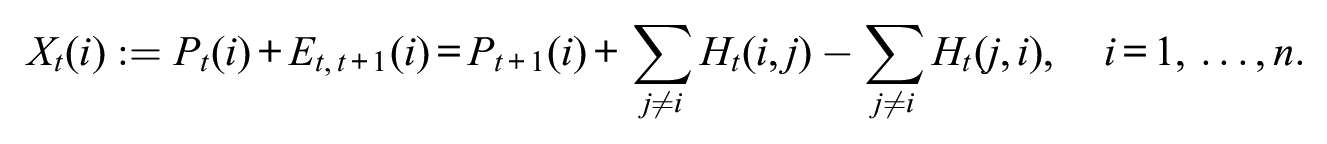
As a prelude to our proposed model, let us assume for now the existence of a probability of migrating from province

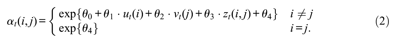
A multinomial regression can be constructed by modeling
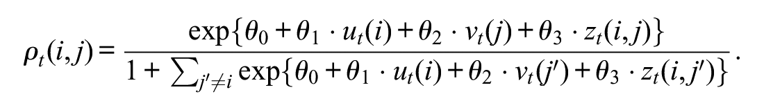
Here,
A limitation of the aforementioned expression may be the deterministic relation between the factors and the migration probability

This time, it is the parameters of the Dirichlet distribution that we model via regression. Specifically,
The resulting model is a Dirichlet-multinomial regression. Observing the expected probabilities

we note that in this model, the vector
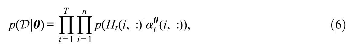
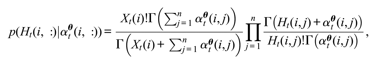
Due to its flexibility, we proceed with the Dirichlet-multinomial regression model described previously. From an inference perspective, the Dirichlet-multinomial specification does not introduce additional complications compared with the multinomial logistic specification. After integrating out

Figure 1 (left) depicts the Dirichlet-multinomial model for a single province and single time step. According to the Dirichlet-multinomial model, people’s decisions within a province are dependent even when conditioned on
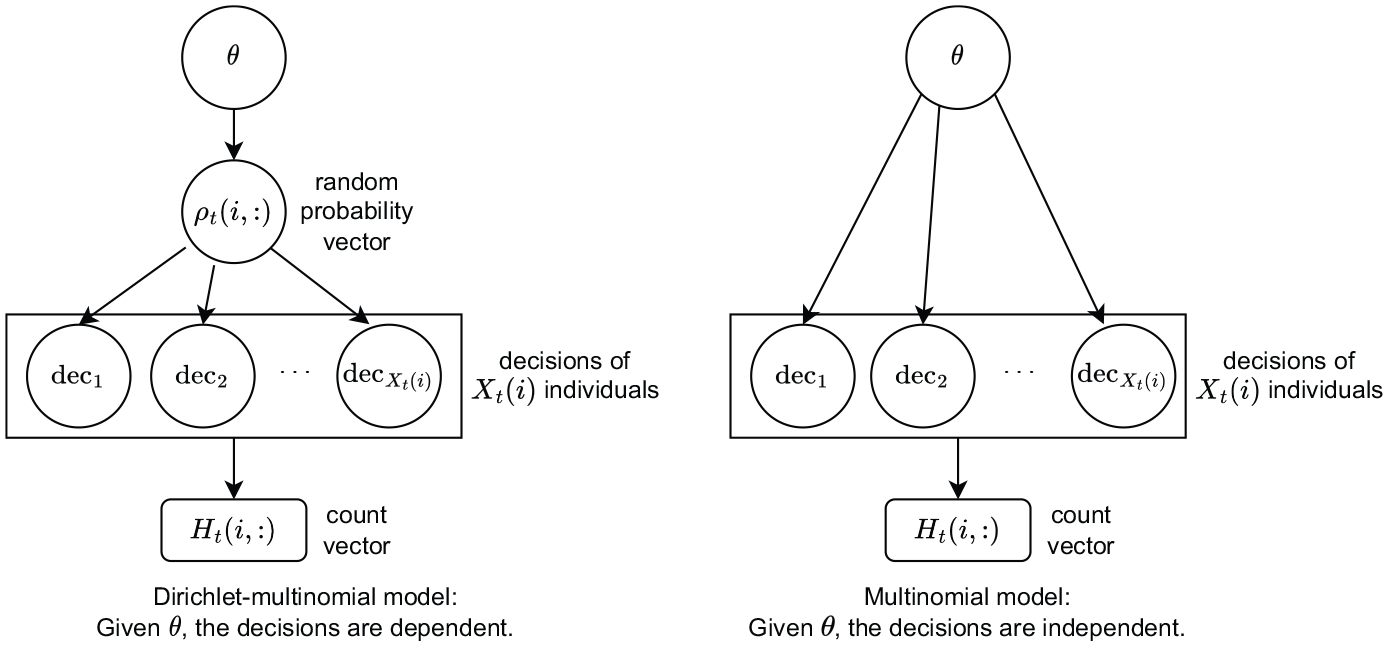
Dirichlet-multinomial model (left) and multinomial model (right).
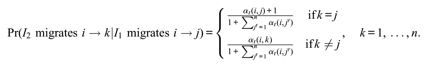
It is possible to quantify the dependency in the Dirichlet-multinomial model in terms of closed-form conditional distributions. For example, given that individual
As another example, given t among

Both examples indicate positive dependency among individuals’ decisions in the same province at the same time period.
The presence of positive dependency between the decisions may be considered another positive feature of the Dirichlet-multinomial model because it captures the possibility that individuals living in the same province may be influenced by each other in deciding to migrate (or not) to a particular destination, for example, through peer effects or familial migration decisions. Furthermore, the strength of this dependency is determined by
Hierarchical Specification
Our data are multilevel, that is, migration from
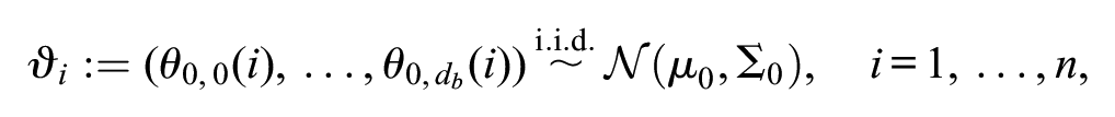
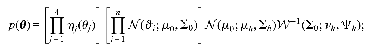
Next, by our aim of Bayesian inference, we build up the prior distributions for the model parameters introduced so far. The parameters

The parameters
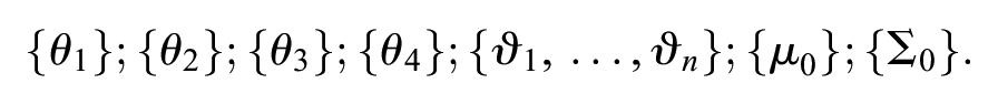
The full parameter vector of the resulting hierarchical model is the
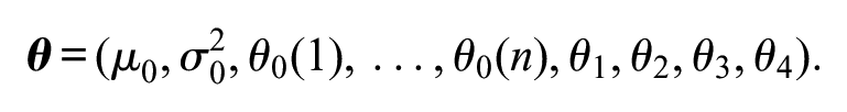
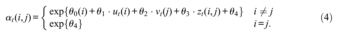
This completes the description of our model of migration in a closed system. We refer to our model whose Dirichlet-multinomial parameters are given by equation (4) as a hierarchical specification because it models the base parameter
One could expand the aforementioned model by making

where the polynomial coefficients for province
and
In our implementations, we will not present results with this polynomial specification. Our results will be restricted to the “random intercept” specification where the base parameters are random across provinces, as in equation (5). This is mainly because province log populations, which are included in the model as predictors, are increasing almost as a linear function of time, rendering the estimation of a separate time slope unnecessary and numerically difficult. We did fit specifications with linear as well as quadratic random time slopes, which did not make noticeable differences in our models, apart from creating convergence problems. That being said, the polynomial specification for the base parameter may be useful in other applications; hence, we will describe our inference method in general and consider the polynomial specification.
Inference
We now turn to our inference method. To quantify the uncertainties in the estimation of
Note that the (adjusted) province populations

Here,
and
where the superscript
where
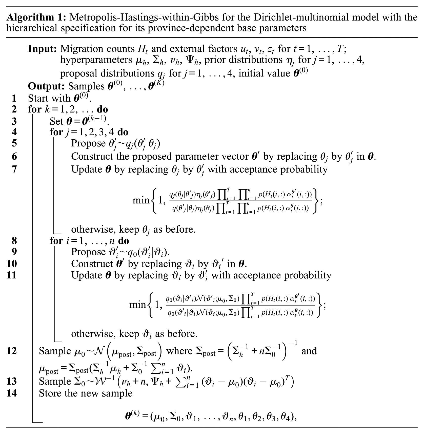
Because the posterior distribution is analytically intractable, we develop an MCMC algorithm (see e.g., Tierney 1994) to sample from the posterior distribution. The developed MCMC algorithm is an instance of Metropolis-Hastings-within-Gibbs. The parameter vector
We note some issues concerning the computational complexity of algorithm 1. While updating each of
Related Methodology
Our model’s closest relative is the one proposed by Guimaraes and Lindrooth (2007). Guimaraes and Lindrooth (2007) developed a Dirichlet-multinomial regression as an extension of the multinomial logistic regression within a discrete-choice random utility framework. They used this to model counts from different groups to multiple destinations (e.g., hospital choice of different groups of patients), where for each group, multinomial probabilities for the destinations are modeled independently with a Dirichlet distribution. Note that our model can also be interpreted from a random utility framework. Consider, for example, the migration decisions of actors at province

Here,
This Dirichlet-multinomial regression model is used by Alamá-Sabater et al. (2017) to explain migration to different parts of Spain from various regions outside of Spain. Our model and Alamá-Sabater et al.’s (2017) model have critical differences. First, Alamá-Sabater et al. (2017) aim to explain how much migration a certain factor “pulls,” hence they only focus on factors of the receiving regions (corresponding to our
A common and notable feature of our model and those previously described is that they rely on the assumption of independence of irrelevant alternatives (IIAs). This assumption implies that the ratio of the probabilities of a single actor moving from
The most common alternative model used to analyze migration is the gravity model (Barthélemy 2011; Expert et al. 2011; Karemera et al. 2000; Poot et al. 2016). In this model, the logarithm of the number of people who moved from
A class of models that share the Bayesian nature of our model and also deal with migration can be found in Azose and Raftery (2015, 2018). The main aim of those models is to forecast country-level future net migration based on past migration via an autoregressive hierarchical model. Azose and Raftery (2018) improve those forecasts by developing a procedure that estimates cross-country correlations in net migration rates. These models differ from ours in that explaining the determinants of migration is not part of their purpose.
The literature on social networks, too, offers a long list of statistical models that can be applied to flows. A canonical model is the exponential random graph model (ERGM; Lusher et al. 2013), which takes the entire data as a network of nodes (e.g., provinces) and edges (e.g., migration flows). In ERGMs, the whole network is modeled as a function of node, edge, and network-level covariates. ERGM enjoys greater generality than our model; using it, one can naturally include various local or global network statistics as explanatory variables and incorporate complex contemporaneous dependencies in the data (i.e., network dependencies in a cross-sectional measurement). The standard ERGM deals with binary edges and cross-sectional settings, so it cannot be directly applied to our problem. ERGM, however, has been extended to deal with longitudinal data (Krivitsky and Handcock 2014) and with count or multilayered networks (Block et al. 2022; Krivitsky 2012; Krivitsky and Handcock 2014; Krivitsky, Koehly, and Marcum 2020) and the more general weighted edges as in generalized exponential random graph models (GERGMs; Desmarais and Cranmer 2012).
An ERGM type of model would be very flexible and general, but it can be challenging to perform inference in ERGMs (Almquist and Butts 2013, 2014), particularly for various generalizations of it. The major challenge may be having to sample the whole network (typically several times) at every iteration, which can only be done approximately, for example, by using Gibbs sampling, unless the network is very small. Note that we also use a Gibbs sampler, but in our case, the inference is much simpler, as we will elaborate. Consequently, while ERGM is generalized to deal with longitudinal data and weighted edges, most applications are constrained to either longitudinal binary networks, cross-sectional networks with weighted edges, or relatively small networks. Indeed, ERGMs have been applied to the study of migration flow networks (Leal 2021; Windzio 2018; Windzio, Teney, and Lenkewitz 2021). However, likely due to those computational complexities, the authors had to simplify the flows so an ERGM can be fitted. For example, Windzio (2018) and Leal (2021) dichotomize flows, and Windzio et al. (2021) use valued edges but impose ordinal categories to migration flows and the data are analyzed only cross-sectionally even though they are longitudinal. Block et al. (2022) develop a weighted ERGM for mobility networks, but the application is restricted to cross-sectional observations. Abramski, Katenka, and Hutchison (2020) successfully apply the GERGM developed by Desmarais and Cranmer (2012) to study refugee migration patterns, but the setup is again simplified with only 12 countries and a cross-sectional analysis.
We also tried to implement an ERGM for count edges (Krivitsky 2012; Krivitsky et al. 2021) to our data. Unfortunately, it failed to converge even for a single year of our migration data, let alone the 10 years our data span. A further issue that needs to be tackled in an ERGM-type model is that the total flow of out-migration is bounded by the population of the origin, and this constraint may be difficult to implement in an ERGM. In our model, these “row-sums” are naturally handled through the Dirichlet-multinomial distribution. We must add that there are exciting recent developments in the ERGM literature, especially the pseudo-likelihood parameter estimation procedures for weighted ERGMs (Huang and Butts 2021), and its applications to migration networks (Huang and Butts 2022) are fast developing. These developments can alleviate the computational and other practical constraints for count data and make ERGMs more feasible for the study of migration flows.
Another class of models developed in the social networks literature that have some similarities with our model comprise the stochastic actor-oriented model (SAOM; Snijders 2001), the dynamic network actor model (DyNAM; Stadtfeld and Block 2017), the relational event model (REM; Butts 2008), and other similar models (Almquist and Butts 2014). These models are designed to analyze longitudinal dynamic binary network data, although extensions for count data exist (Stadtfeld et al. 2017a). In the actor-based SAOM and DyNAM, two processes are modeled separately: the timing of an event (e.g., a tie to be formed) and the target of the event (e.g., whom a person sends a tie), which is modeled with a multinomial specification. In the tie-based REM, the timing and position of an event (e.g., which two nodes are connected) are modeled simultaneously. In our model, the exact timing of migration is unknown, apart from it taking place during a given year. Moreover, many migration flows take place during a given year. To apply the dynamic network models discussed here, one needs to be able to calculate the conditional distribution of the migration data of a year given the state of variables in the previous year. This is not available in our case because we do not know the times of individual migration events and integrating them out is analytically intractable. One can only approximate those conditionals, making this class of models inconvenient for us to apply in our case.
A final class of models, developed again mainly in the social networks literature, includes latent space (Hoff et al. 2002; Hoff and Ward 2004) and latent factor (Minhas et al. 2019) models. Most recently, and perhaps most relevantly, Minhas et al. (2019) described a latent factor model in which cell outcomes in a matrix (e.g., migration flows in our case) are modeled as a function of the sender and proposer characteristics plus a latent factor matrix. The elements of this matrix are the sender and receiver latent factors multiplied by a sender-receiver pair parameter. This latent multiplicative factor captures higher-order dependence structures that are not explained by the observed covariates included in the model. Minhas et al. (2019) then proposed a Bayesian estimation procedure that assumes certain prior distributions for the parameters, including the elements of the latent factor matrix. This class of models is very flexible, too. Applications, however, are often restricted to binary data, although an extension to the multinomial and count data is possible. In addition, diagonals are often not modeled explicitly (see e.g., Minhas et al. 2019), and it is not straightforward to constrain the row-sums that are bounded in our data by the province populations.
Overall, we argue that the methodology and the modeling approach of these relational and network models are too general for our problem. In contrast, our model is directly related to the migration (and other similar) flows and can be derived from a small number of assumptions (e.g., multinomial probabilities and independence of the actors in different provinces). For example, staying within the notation in our article, the SAOM in Snijders (1996) takes
Note that in our model, a person’s decision in province
We should also add that the conditional independence assumption of our model is less problematic, the more frequent the temporal measurements are. We have annual migration data, which we believe is frequent enough given that most migration decisions are not made on a whim. If, however, the researcher has only cross-sectional data or data that are collected very infrequently, such as decades apart, then complex dependencies in migration flows between actors from different provinces may not be captured in our model. In such cases, however, the researcher would have a simpler data structure for which the more complex count ERGM-type models may work better.
We believe the models developed in the social networks literature reviewed previously are rich, very general, flexible, and in principle can be applied to the type of data we have here, especially given the rapidly developing work on estimation in valued ERGMs. A systematic comparison of all possible alternative modeling approaches, however, is beyond the scope of the current study.
Determinants of Migration
We now move to the substantive discussion of the expected drivers of migration and describe the Turkish context to which our data belong. Migration is a complex phenomenon with multiple causes, hence there is no single theory for it. A nonexhaustive list of the determinants of voluntary migration can be grouped into economic, demographic, geographic, cultural, and social network factors (Boyle et al. 1998). In classical economic theory, income maximization relative to the costs of moving is a key driver of migration (Borjas, Bronars, and Trejo 1992). Economic prospects, such as a high per capita income, employment opportunities, or wages, should pull migrants. Conversely, poor economic prospects should push migration.
Migration flows are also shaped by population. The larger the population of the origin and the destination, the larger the flow will be between the two (Barthélemy 2011; Levy 2010). This prediction is due to the empirical regularity that flows correlate positively with stocks in either direction (Poot et al. 2016). A large population means there is more capacity to send and receive migrants.
Increasing population may increase migration flows, but the spatial distance between the origin and the destination constrains it. Next to the gravity model, spatial network models, too, show that distance affects ties between individuals (see e.g., Butts et al. 2012). The effect of spatial distance operates via various channels (Schwartz 1973). First, it directly increases the cost of moving, a key factor in the economic model of migration. Second, it hinders maintaining contact with friends and family in one’s origin country, hence imposing a psychological cost on migration. Third, the larger the spatial distance, the lower the information flow between the origin and destination. A lower information flow means it is more difficult to hear about available opportunities at the destination. The combined effect of population and spatial distance on migration is sometimes referred to as the “gravity law”: The “mass” (i.e., population) of the origin and the destination relative to the spatial distance between the two determines flows (Barthélemy 2011; Levy 2010).
The gravity law focuses exclusively on spatial distance, but cultural or linguistic distances constrain migration, too. Similarity between the origin and destination concerning language and religion, for example, improves migrants’ labor market integration (Van Tubergen, Maas, and Flap 2004; Windzio 2018). Furthermore, cultural similarity facilitates migration due to homophily (McPherson, Smith-Lovin, and Cook 2001) and by reducing discrimination and acculturation costs for migrants (Van Tubergen et al. 2004).
Finally, social networks are highly consequential for migration (Massey and España 1987). This is true for the social network of the individual migrant (Massey and España 1987) as well as macro-level network features of the origin and destination (Levy 2010; Windzio 2018). Knowing people who migrated previously reduces the cost of migration for a prospective migrant. A social network in the destination can introduce a prospective migrant to possible employers, suggest places to live, offer information on vacancies, and provide social support that reduces the psychological costs of migration (Massey and España 1987). These effects make migration self-perpetuating: The more migration there is from
The reverse should be true as well: The more migration there is from i to j, the more migration is expected to take place from j to i. In other words, one expects a reciprocity effect. This is first due to return migration (Borjas and Bratsberg 1996; Danchev and Porter 2018). But once a link is established between i and j through large-scale migration, natives in
Other network characteristics, such as betweenness centrality (Freeman 1977) and in-degree assortativity (Newman 2002), will also affect migration. The betweenness centrality of a node in a network indicates how many (weighted) shortest paths pass through the node. A high level of betweenness centrality of an area implies that the area acts as a migration hub. This also means there is high diversity because people from different origins come to the area and likewise go to different destinations. This may offer new economic opportunities that attract further migration. Indeed, using an instrumental variable design, Damelang and Haas (2012) show that in Germany, cultural diversity enhances immigrants’ labor market success. Finally, if two provinces
Internal Migration in Turkey
Historically, Turkey has sent a large number of emigrants to Europe. Most research has thus focused on Turkish immigrants’ integration into Europe. Since the 1980s, however, emigration from Turkey to Europe has decreased (İçduygu and Sert 2009). Far larger shares of the population migrate internally. Our data show that annually, around 2.5 million people migrate between the 81 provinces of Turkey. Annual emigration abroad, on the other hand, is around 250,000.
Work on the determinants of internal migration in Turkey is scarce (Koramaz and Dökmeci 2017). Most of the existing research has been carried out by urban planners whose main focus is on spatial issues (Filiztekin and Gökhan 2008). Almost all existing studies analyze data up to the year 2000, that is, the last year a population census was conducted. Studies that use more recent migration data are mainly descriptive; for example, Akın and Dökmeci (2015) classify the 12 regions of Turkey based on interregional migration patterns.
Gedik (1997) shows that starting from the 1980s, the vast majority of migration in Turkey takes place from city to city as opposed to rural to urban. Evcil, Kiroplu, and Dokmeci (2006) confirm this pattern. As expected, economic factors such as per capita gross domestic product (GDP), wages, industrial workforce, and unemployment rates are important determinants of migration (Filiztekin and Gökhan 2008; Gezici and Keskin 2005). Evcil et al. (2006) argue that GDP differentials are one of the most important drivers of internal migration.
In line with the gravity law, populations in the origin and destination are positively associated with migration flows (Filiztekin and Gökhan 2008; Gezici and Keskin 2005). The findings on the second component of the gravity law, namely, spatial distance, are equivocal. Gedik (1997) argues that beyond the immediate neighboring cities, the effect of spatial distance on migration is minimal. Koramaz and Dökmeci (2017), however, report that after peaking at a distance of 200 to 400 kilometers, migration decreases rapidly as spatial distance increases. Koramaz and Dökmeci (2017) also report that in provinces in the east, most of which have large shares of Kurds, the effect of spatial distance is less pronounced.
Earlier studies also indicate the importance of social networks. Gedik (1997) shows that previous migrants who are friends or relatives from the same area are as effective as economic factors in facilitating migration. Filiztekin and Gökhan (2008) use the stock of earlier migration between
Other important social forces may affect internal migration in Turkey. The first is politics. Aksoy and Billari (2018) and Aksoy and Gambetta (2021) show that provinces and districts ruled by Erdoğan’s AKP (Justice and Development Party) are more efficient in providing local services and social assistance than are those controlled by the opposition. This can potentially lead to “welfare migration” from opposition to AKP municipalities. Aksoy and Billari (2018) do not find evidence for such welfare migration, but migration is not their focus, and hence their analysis is rather descriptive. Political polarization is also rife in Turkey. In a recent poll, 78 percent of respondents did not “approve of their daughter marrying a supporter” of a party other than their own (Erdoğan and Semerci 2017). We are not aware of any previous work that systematically focuses on the effect of politics and political distance on migration in Turkey. Yet, we expect Turkey’s political divides play an important role in migration decisions.
A further potentially important factor is ethnicity. Sizeable Kurdish populations live in Turkey’s large cities. This is due to both economic and forced migration. Violent conflicts in the 1990s resulted in the forced displacement of Kurds (Ergin 2014). Kurds tend to have higher levels of unemployment, poverty, and fertility (Koc, Hancioglu, and Cavlin 2008), factors that traditionally push people to migrate. Due to historical and political reasons, data on ethnicity in Turkey are scarce; no population census since 1965 includes a question on ethnicity (Koc et al. 2008). Hence, it is unknown if Kurdish migration is particularly high once economic factors and population are accounted for. In this study, we will provide the first comprehensive test.
Data and Descriptive Results
Data and Variables
We compiled a new data set for this study. All variables are at the province level, and there are 81 provinces. We obtained all variables from the Turkish Statistical Institute (TurkStat), except the proportion of Kurds in a province, which we estimated from two representative surveys.
Dependent variable: migration counts
The number of individuals who moved from one province to another in a given year is available from TurkStat from 2009. These data come from Turkey’s Address Based Population Registration System (ABPRS), which replaced the census in 2007. By law, each Turkish citizen is required to be registered at a single primary address. Any change in one’s primary address must be updated in ABPRS within 20 working days, online or in person. Not complying results in penalties. There are other incentives to keep the primary address up to date; for example, school access is determined by residence, and any official communication takes place via the registered address. Migration that is not yet registered in the system is not captured by these data. Hence, our dependent variable should be interpreted as “official” internal migration.
We also calculate the number of people who did not migrate. We do so by subtracting net migration (out-migration – in-migration) from the population of a province in a year. We apply a correction by adjusting for the number of births, deaths, and those who register for the first time in the province in a given year. This gives us an
Explanatory variables
We predict migration with the following explanatory variables. In our model, all dynamic (i.e., time-varying) explanatory variables are lagged by one year. As indicators of economic prospects, we use annual provincial GDP per capita and the unemployment rate. Unemployment rates are only available at the Nuts-2 level, which comprises 26 large regions. As elements of the gravity law, we use annual population in and the spatial distance between provinces. Spatial distance is measured as the driving distance in kilometers between province centers. To measure the political distance between provinces, we calculate the absolute difference in vote shares of the political parties in the 2004, 2009, and 2014 mayoral elections. Political distance is a dynamic variable.
We calculate the following network characteristics using the (one-year lagged) migration matrix. The self-perpetuating nature of migration is captured by the number of people who migrated from
We also use the proportion of municipalities in a province that is controlled by the AKP after the 2004, 2009, and 2014 elections as a dynamic variable. This variable has a [0, 1] range corresponding to the provinces in which AKP controls none or all of the municipalities in a province in a given year.
We estimate the percentage of Kurds in a province as a dynamic variable. There is no official data on ethnicity, so we use Turkey’s Demographic and Health Survey 2008 and 2013 waves (Koc et al. 2008). Both surveys are representative and sample women of reproductive age (15–49; Hacettepe University Institute of Population Studies 2008–2013). The survey includes a question about the respondent’s mother tongue, which we use to identify if someone is Kurdish. We use the 2008 and 2013 waves to estimate the proportion of Kurds in a province in and before those years.
To facilitate estimation and interpretation, we normalize all explanatory variables, except time, to the [−1, 1] range by centering around the mean and dividing by the maximum of the absolute of the centered values, hence we attain one of the
Descriptive Results for Migration
Figure 2 shows out-migration and in-migration in the 81 provinces of Turkey. The figure shows the absolute level of migration, migration as the percentage of the number of inhabitants at the start of the year, and the 2018 to 2009 difference in the latter. We see that large provinces, such as İstanbul, Ankara, İzmir, Adana, and Antalya, have high levels of out-migration and in-migration (see Figure 3 for province names). This is in line with the gravity law. There is almost a perfect correlation between out-migration and in-migration levels across provinces.
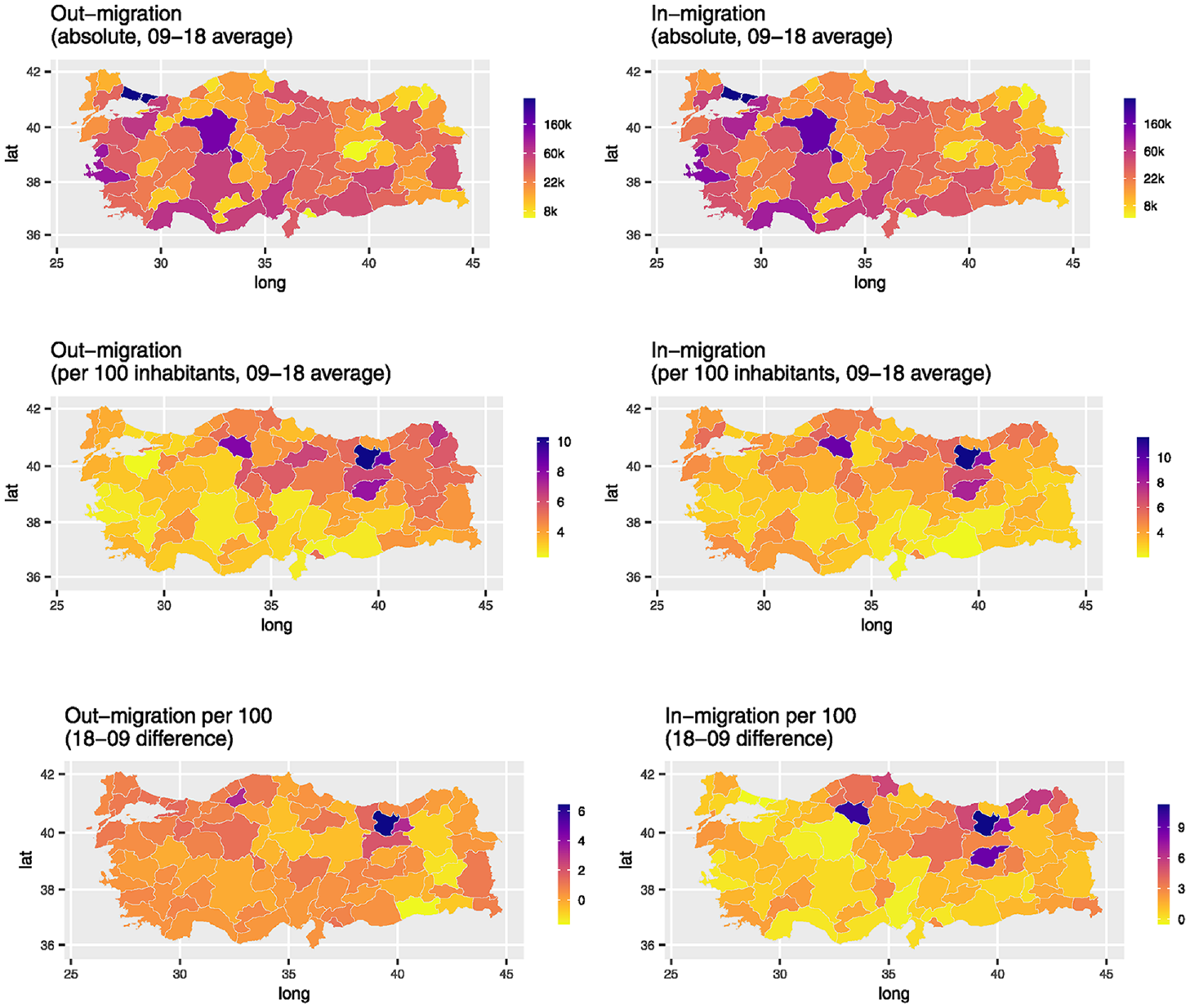
Absolute, per 100, and change in per 100 between 2018 and 2009 in out-migration and in-migration per province.
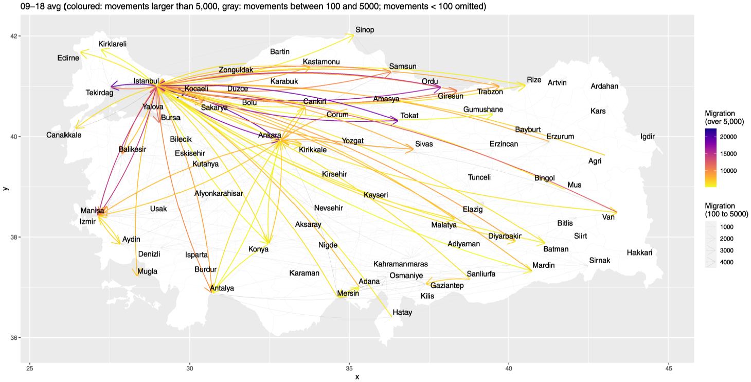
Migration flows between provinces.
Migration as a percentage of the number of inhabitants, however, shows a different pattern. Proportional to their populations, large provinces (e.g., İstanbul, Ankara, İzmir, Adana, and Antalya) have relatively low migration. Smaller provinces in the center-east, such as Gümüşhane and Tunceli, have the highest migration per capita. The difference between absolute and relative migration will become important when we present our model estimates. The bottom panels of Figure 2 show that on average, the change in out-migration per capita is rather stable. However, it is slightly negative in some places and slightly positive in others; the largest change is in Gümüşhane.
Figure 2 shows only the origins and destinations of migration. Figure 3 shows absolute migration flows. In Figure 3, we omit small flows for clarity. These small flows will be part of the analyses in the next section. Figure 3 shows that İzmir, Anlatya, Tekirdağ, Ordu, Tokat, and Ankara are popular destinations, especially for individuals from İstanbul. Local clusters, such as Şanlıurfa, Konya, Gaziantep, Adana, and Mersin, also attract and send migrants. Finally, Figure 4 shows the bivariate correlations for the one-way (i.e., variables defined for a province, “node” characteristics) and two-way (i.e., variables defined for a pair of provinces, “edge” characteristics) factors. As expected, many predictors are correlated.
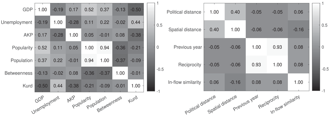
Sample correlation matrix for the one-way and two-way factors.
Results
We now provide the results of the implementation of our methodology using the migration data described in the previous section. We performed the experiments in MATLAB, version R2021b. All data and the code that produce the results are available (anonymized for peer review) at https://github.com/SocNetMigration/MigNet-MATLAB-code.git. This replication package also includes guidelines for preparing other data for our model.
Model Estimates
We implemented the sampling method in algorithm 1 to estimate
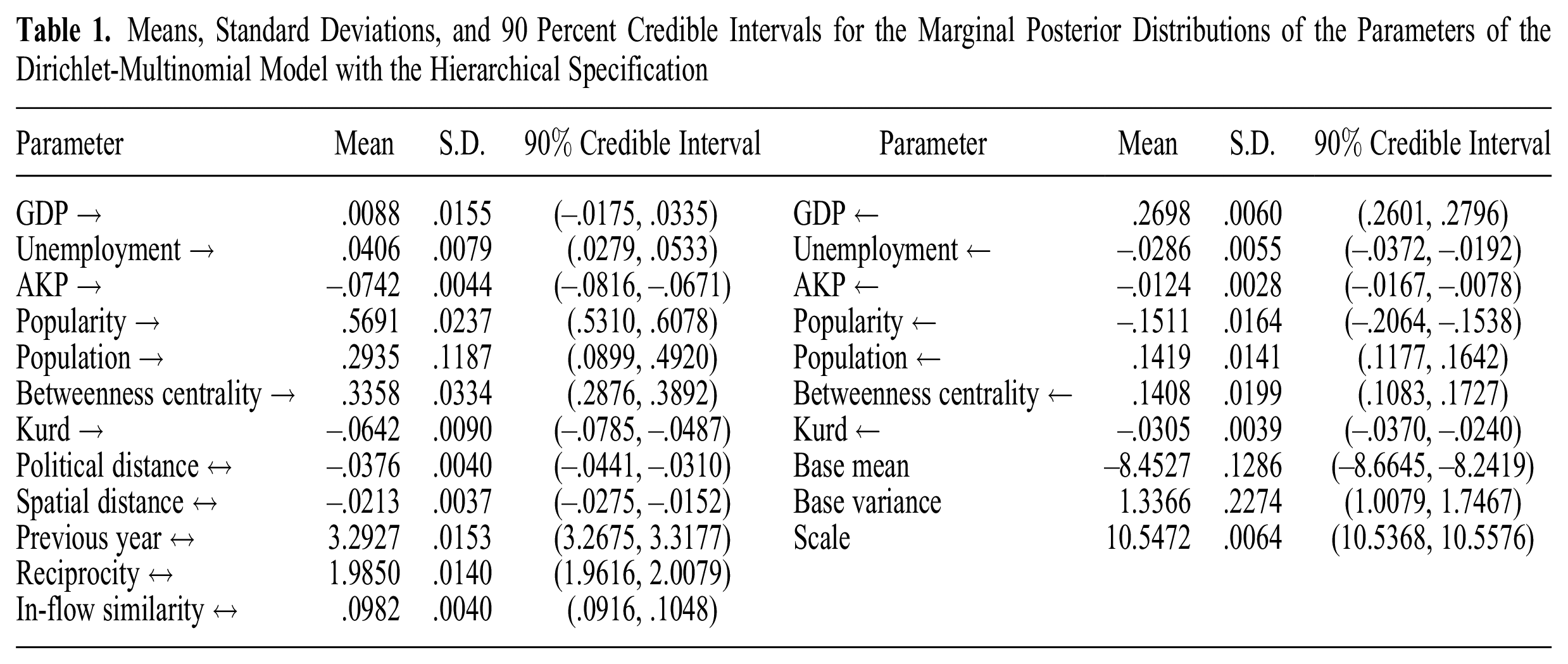
Figure 5 shows the box plots for the estimated marginal posterior distributions of the coefficients for our predictors of migration. Table 1 displays the means, standard deviations, and 90 percent credible intervals of those parameters and of the random intercept and the “scale” parameter of the Dirichlet-multinomial model (see equations [2] and [4]). The correlation structure in the posterior distribution for
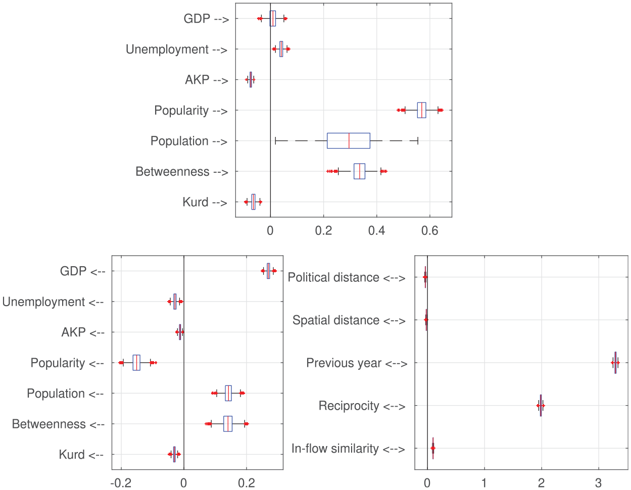
Box plots of marginal posterior distributions of factor coefficients in the hierarchical (random intercepts across provinces) Dirichlet-multinomial model.
Means, Standard Deviations, and 90 Percent Credible Intervals for the Marginal Posterior Distributions of the Parameters of the Dirichlet-Multinomial Model with the Hierarchical Specification
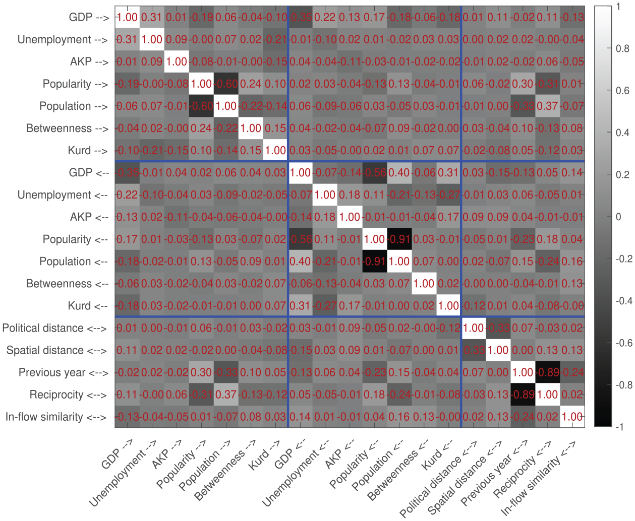
Posterior correlation matrix.
The correlation structure in the posterior in Figure 6 is in line with the correlation matrix of the predictors given in Figure 4. A comparison of these two figures shows the typical trend that a positive correlation between two predictors yields a negative correlation between their coefficients in the posterior and vice versa, as expected. This justifies the general cautionary rule, which applies to almost all multivariate models, that the effects of correlated predictors should not be considered in isolation from each other.
The results are mostly in line with theory. Unemployment (→) in the sender province is positively associated with out-migration, and unemployment (←) in the target has a negative association with in-migration. GDP (→) in the sending province does not seem to have a strong association with out-migration, whereas GDP (←) in the target is strongly and positively associated with in-migration.
Regarding the elements of the gravity law, a large population (→) is associated with a higher probability of out-migration: the posterior mean of its coefficient is .29. Population (←) in the target also has a very strong positive association with in-migration. We also find a negative association between spatial distance (↔) and migration. These results are in line with the gravity law. We also find a negative association between provincial political distance (↔) and migration. Interestingly, the size of the coefficient for political distance is slightly higher than that for spatial distance.
As expected, network characteristics are strongly associated with migration. Migration from
We find that the strength of the AKP in a province is negatively associated with both out-migration (→) and in-migration (←), although its coefficient is small in both cases. This shows that migration out of and into AKP-dominated regions is low. Together with the strong negative coefficient for political distance, this finding further indicates the negative association of political divides with migration.
Finally, the proportion of Kurds in a province is associated negatively with both out-migration (→) and in-migration (←). Although its coefficients are low in the absolute sense, negative values are inconsistent with the common belief that migration is a Kurdish phenomenon. Note, however, that the outcome is all migration from and to a province, Kurdish or otherwise. Hence, the evidence here is indirect. Nevertheless, if Kurds were much more mobile than Turks and other ethnicities, as the common belief suggests, one would expect a positive effect of the proportion of Kurds in a province on out-migration.
The coefficients for ← and ↔ factors can be interpreted in terms of relative probabilities of attracting migration from a given province. For example, suppose the maximum observed GDP value is normalized to
Table 1 also shows the mean and the variance of the intercept, which is random across provinces. We see considerable variability in the levels of out-migration probabilities across provinces, the largest in Bayburt and the smallest in Istanbul. Figure 7 shows the posterior distribution of the intercepts per province, estimated with our hierarchical specification. These provincial variations somewhat match the descriptive statistics given in Figure 2, although they are not equal because these intercepts are obtained after controlling for the predictors of migration.
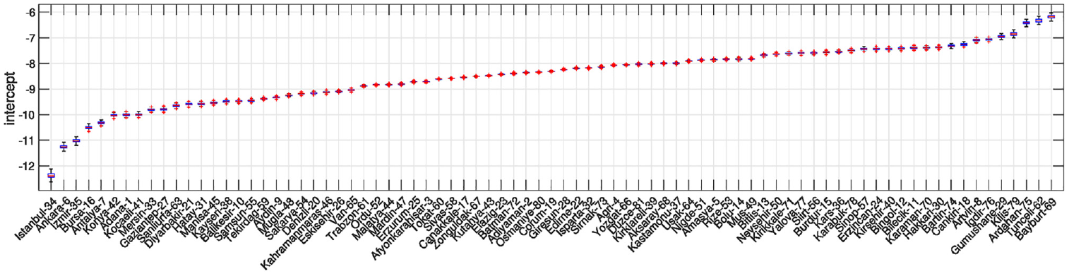
Box plots of the marginal posterior distributions of random intercepts for provinces in the hierarchical specification of the Dirichlet-multinomial model.
Additional estimation results
Some scholars argue that controlling for the lagged dependent variable accounts for path dependency or autocorrelation of residuals in panel regressions, although it may also bias downward the coefficients for other explanatory variables (Keele and Kelly 2006). This issue has been shown to apply to temporal ERGMs, too (Block et al. 2018). To address this potential issue, we fitted our models after excluding variables that are calculated from past migrations: popularity, betweenness, previous year, reciprocity, and in-flow similarity. The results after excluding these variables are given in Appendix B.2.
These additional results show that including the measures based on migration in the previous year generally does not suppress the coefficients of the other variables. In fact, for some variables, the estimated coefficients are somewhat smaller after excluding the lagged measures (e.g., AKP ←). Coefficients do increase, in absolute value, for some variables (e.g., GDP →, Kurd ←) after excluding lagged variables. But because of a lack of general suppression of coefficients due to including measures based on lagged values of migration, we conclude that this issue is not particularly problematic in our case. Note that one expects differences in the coefficients of variables that are estimated before and after the inclusion of lagged migration variables due to the conditional nature of the Dirichlet-multinomial regression, which we observe. Additionally, as shown in Appendix Table B1, the exclusion of lagged measures reduces the predictive performance substantially, further suggesting the need for including them in the model.
Comparison with the Gravity Model in Terms of Predictive Power
The gravity model assumes a linear regression for the nondiagonal log-migration counts. The essential factors of the gravity model are population and distance, but one could easily include other one-way and two-way factors. Therefore, for fairness in comparison, we constructed a gravity model that includes all the factors considered in our model. This corresponds to the following relation for

where the sum on the right side serves as the base parameter as before;
We compared the gravity model and the Dirichlet-multinomial model in terms of their out-of-sample predictive performances with the following process. Recall that the total data consist of 10 consecutive years between 2009 and 2018. For every year, we excluded its migration data and used the rest of the years to train the model. The training results are then used to predict the migrations in the excluded year. For the Dirichlet-multinomial model, we ran algorithm 1 (or variants of this for the global and random effects intercepts) to obtain samples from the posterior distribution of
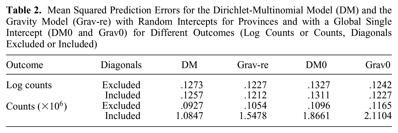
The results (see Table 2) show that the Dirichlet-multinomial model has better performance than the gravity model in predicting migration counts. Prediction errors for the Dirichlet-multinomial for count outcomes are consistently lower than that for the gravity model both when we include and exclude the diagonal (nonmigration) values in the predicted outcome. When the log-counts are considered, the gravity model performs slightly better than the Dirichlet-multimonial. This suggests the gravity model is generally mispredicting large flows. As an aside, the mean absolute error of our hierarchical model for all counts including nonmigration is only 108.6, which corresponds to less than .05 percent of the standard deviation of migration counts. This shows that our model predicts migration flows reasonably well. Also note that random province-specific intercept parameters improve the performance, and hence the random effects do not lead to overfitting.
Mean Squared Prediction Errors for the Dirichlet-Multinomial Model (DM) and the Gravity Model (Grav-re) with Random Intercepts for Provinces and with a Global Single Intercept (DM0 and Grav0) for Different Outcomes (Log Counts or Counts, Diagonals Excluded or Included)
We also compared the predictive performance of our method with that of a simpler variant that excludes variables based on the previous year’s migration flows (see Appendix Table B1). The results show that the exclusion of lagged measures hampers predictive performance substantially, pointing to the need to include them in the model as we do.
Baseline Probability of Migration and the Predictive Accuracy of the Gravity Model
The aforementioned results show that our model outperforms the gravity model in predicting migration counts. We conjecture that one of the main reasons for the relatively poor performance of the gravity model in predicting migration counts is because the gravity model fails to capture the mechanistic relationship between migration out-flows to different targets from the same origin (e.g., due to competition between different targets for a constant number of possible migrants from a given origin). This drawback increases as the share of a population that migrates relative to those that do not increases. This is because the smaller the share of people in an origin that do not migrate (hence the larger the share of those who migrate), the larger the (negative) correlation between migration flows to different destinations, and because the gravity model does not capture those correlations naturally, the predictive accuracy of the gravity model will be lower.
To demonstrate the mechanism explained so far and help understand the predictive performance of the gravity model vis-a-vis ours better, we carry out a Monte Carlo simulation, where we test the predictive performances of the Dirichlet-multinomial model and the gravity model on simulated data sets. In our simulation, we randomly generate migration flows using two separate processes. In the first process, we generate migration flows from the Dirichlet-multinomial model with
In this simulation, our aim is to better understand how the predictive accuracy of the gravity model depends on the baseline probability of out-migration, rather than comparing our model with the gravity model in all possible data-generation scenarios. Nevertheless, because we generate the migration counts from a Dirichlet-multinomial model, one may argue that the data-generation process does not do justice to the gravity model. Hence, in a second process, we generate migration counts from a multivariate normal distribution obtained by randomly “perturbing” the Dirichlet-multinomial model. Specifically, for every

that is, we distort the covariance matrix to deviate from the Dirichlet-multinomial model while still keeping the negative correlation among the counts. The counts drawn from the multivariate normal distribution are then rounded to the nearest integers and truncated at the zero lower bound. Finally, we readjust the population according to the final values of the counts. As in the first process, in this second process,
Figure 8 shows the results of our Monte Carlo simulations. The figure confirms our conjecture as to the reasons for the gravity model’s relatively poor predictive performance. As the baseline probability of migration increases (corresponding to larger
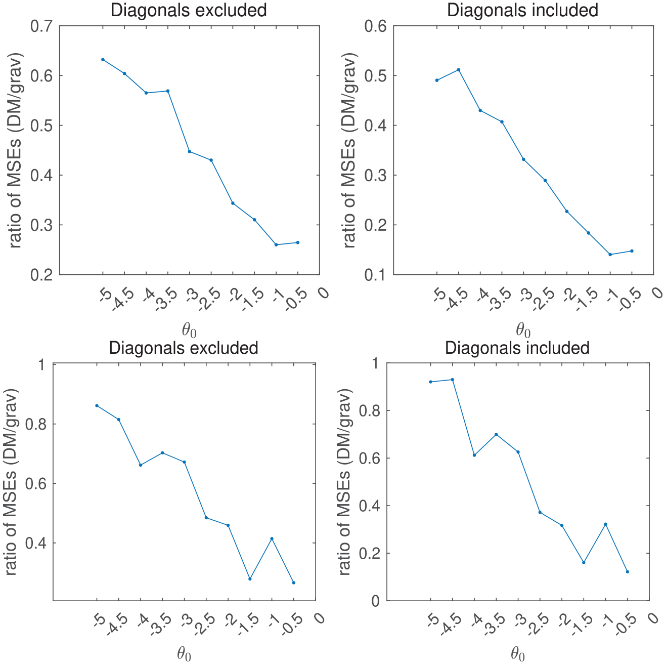
Predictive performance of the gravity model relative to the Dirichlet-multinomial model on simulated data.
Discussion and Conclusions
In this study, we proposed a Dirichlet-multinomial model and a Bayesian inference method to analyze the interdependent flows. We applied the developed methodology to analyze the dynamic migration flows of the 81 provinces of Turkey from 2009 to 2018. Our study offers methodological and substantive contributions to the literature.
On the methodological front, our Dirichlet-multinomial model alleviates several shortcomings of the popular models applied to migration flows. First, our model naturally captures systemic effects. That is, unlike the gravity model, our model incorporates the effects of the characteristics of all alternative destinations on a decision to migrate to a specific destination. Second, our model accounts for nonmigration. The alternative to ignoring nonmigration and conditioning the results on migration having taken place, which is a common practice in the literature, results in selection on the dependent variable. Third, our model adheres to the natural boundary of migration and the mechanistic relationship between migration and nonmigration. That is, out-migration and in-migration change the populations of the origin and the destination, and the total number of out-migration cannot exceed the population of the origin in a given period. Our model naturally incorporates these phenomena. Fourth, our model lends itself to an estimation method that is computationally much simpler than many of its alternatives. The computational simplicity allows us to expand our model with a hierarchical specification that captures variations in the baseline of, and potentially also longitudinal changes in, migration probabilities.
To demonstrate these advantages, we carried out an out-of-sample prediction comparison of our model vis-a-vis the gravity model, one of the most common models used in the migration literature. The gravity model ignores systemic effects, and it typically ignores nonmigration and the mechanistic relationship between populations, nonmigration, and migration flows. We showed that our model consistently outperforms the gravity model in predicting migration flow counts.
We also showed through Monte Carlo simulations that the predictive accuracy of the gravity model worsens as the ratio of migrants to nonmigrants increases. Conversely, as the ratio of migrants to nonmigrants approaches zero, the predictive accuracy of the gravity model converges with that of our model. This implies that when migration is a much rarer event compared to nonmigration, the gravity model would perform reasonably well.
Note that while we framed our model within a migration setting, and indeed we developed it to understand migration flows and their determinants, the model is more general. It can be applied to any setting that involves discrete dynamic flows between a finite number of origins and destinations.
Several models developed in the social networks literature, which are very general and flexible, can, in principle, be applied to dynamic flows with some adjustments. These include ERGMs and their various extensions for count data or longitudinal data, REMs, DyNAMs, SAOMs, and latent space and latent factor models. We discussed those models in detail and compared them with ours. While they are indeed very powerful and flexible, we argued they may be too general for our problem at hand. Our method provides a straightforward approach to model dynamic flows while offering computational simplicity and at the same time taking into account key features of and dependencies in the data.
The computational simplicity of our model rests on the assumption that migrations from different origins at a given time point are independent, conditional on the covariates, which can include those based on previous migration flows. Note that this conditional independence assumption is about decisions in different provinces, and our model incorporates possible positive correlations between migration decisions within the same province. We believe this assumption is not unrealistic in our longitudinal context. When individuals are deciding whether to migrate in a given time point, they may not consider or indeed be aware of the migration decisions of others outside their provinces at the same time point. Moreover, dependencies among migration probabilities that may violate this assumption can be explained away, to a certain degree, by including in the model the predictors that are the likely causes of that dependence. For example, if one expects a “herding” dynamic for migration (i.e., people in different provinces imitating each other in migrating to a specific destination), this factor can be added to the model by adding a destination popularity factor based on previous migration flows into the destination, as we do in our analysis. In other words, because we have longitudinal data, we can condition current flows on earlier flows, which makes the conditional independence assumption more plausible.
Our model allows for further extensions. In particular, in our hierarchical specification, we include random intercepts for out-migration (i.e., for sending provinces). One can include such random effects for the receiving provinces, too. This would result in a cross-classified model (Snijders and Bosker 2011). In fact, we fitted this cross-classified version. The parameter estimates and the predictive performance of our model hardly changed. Yet the receiver random effects increased the computational complexity of the model substantially. This is because in a cross-classified model, each of the n random intercepts of the receiving provinces would affect the Dirichlet-multinomial probabilities for all provinces. Thus, the acceptance probability in the estimation, which is needed to accept or reject a proposed update for each of those parameters, would require the computation of the whole product in equation (6). Note that this is in stark contrast with the update of the intercept of the sending provinces, for which we calculate a single Dirichlet-multinomial probability for each
Overall, we contribute to the literature methodologically by providing a viable alternative for analyzing migration and other types of flows. Our study also offers substantive contributions to the migration literature. Far greater shares of populations are affected by internal migration than by international migration. Most past research, however, focuses on the latter. Using a new data set and a model, we analyze interprovincial migration in Turkey. Our results largely confirm the existing theories of migration: economic prospects, population, spatial distance, and network characteristics shape the flow of internal migration in Turkey. We also offer several novel findings.
First, we register that political distance between provinces (measured using electoral results) is negatively associated with migration flows. This negative association is even stronger than that between spatial distance and migration. Moreover, we find that the strength of the AKP (Justice and Development Party) in a province is negatively associated with out-migration and in-migration. These findings imply that political divisions in the country contribute to the sorting of province populations. This association between politics and migration, in turn, may accelerate the political polarization between Turkey’s provinces, which is already rife.
We also provide, to our knowledge, the first systematic test of whether the proportion of Kurds in a province is associated with migration. Kurds are affected by higher levels of unemployment and poverty and have higher fertility rates. These factors are traditionally associated with migration. Indeed, there has been large-scale Kurdish migration to western parts of Turkey. Our analysis, however, shows that conditional on the factors we include in our model, the share of Kurds in a province has a small negative association with migration. While these findings should be interpreted with caution, as the independent variable is the share of Kurds in a province and the outcome is migration across all ethnic groups, a lack of a positive coefficient suggests internal migration in Turkey is not a predominantly “Kurdish phenomenon.”
Footnotes
Appendix
Acknowledgements
We thank Zsofia Boda and Burak Sönmez for their comments on earlier drafts.
Authors’ Note
The authors contributed equally to the manuscript.
Funding
The authors disclosed receipt of the following financial support for the research, authorship, and/or publication of this article: Aksoy acknowledges financial support from the British Academy (Grant No. SRG20/200045).