Sage Journals: Discover world-class research

Abstract

Researchers increasingly use aggregate relational data to learn about the size and distribution of survey respondents’ weak-tie personal networks. Aggregate relational data are collected by asking questions about respondents’ connectedness to many different groups (e.g., “How many teachers do you know?”). This approach can be powerful, but to use aggregate relational data, researchers must locate external information about the size of each group from a census or administrative records (e.g., the number of teachers in the population). This need for external information makes aggregate relational data difficult or impossible to collect in many settings. Here, the authors show that relatively simple modifications can overcome this need for external data, significantly increasing the flexibility of the method and weakening key assumptions required by the associated estimators. The key idea is to estimate the size of these groups from the sample of survey respondents, rather than relying on external sources of information. These methods are appropriate for using a sample survey to study the size and distribution of weak-tie network connections. They can also be used as part of the network scale-up method to estimate the size of hidden populations. The authors illustrate this approach with two empirical studies: a large simulation study and original household survey data collected in Hanoi, Vietnam.

Keywords

aggregate relational data network scale-up networks sampling

Many population-level insights about social networks come from surveys that investigate relatively strong ties, such as the ones produced by name generators (e.g., Fischer 1982; Marsden 2005; Perry, Pescosolido, and Borgatti 2018). Comparatively few studies have examined weaker ties, but there are several reasons why weak ties can be important: first, information about weak ties is needed to understand homophily, segregation, and social capital (e.g., DiPrete et al. 2011; Lubbers, Molina, and Valenzuela-García 2019; McCormick, Salganik, and Zheng 2010; Zheng, Salganik, and Gelman 2006); second, weak ties are hypothesized to play a critical role in important social processes, such as social support, information diffusion, and social influence (Granovetter 1973; Lubbers et al. 2019); and third, reports about weak ties can be instrumentally useful in trying to measure the size and composition of hidden and hard to reach populations through network scale-up and related methods (e.g., Bernard et al. 2010; Feehan and Salganik 2016a; Maltiel et al. 2015).

Researchers have developed several methods to try and estimate the size of weak-tie networks from a sample of people, but this has proved to be a challenging problem (de Sola Pool and Kochen 1978; Killworth, Johnsen, et al. 1998; Killworth, McCarty, et al. 1998; McCarty et al. 1997, 2001). One promising approach is based on collecting aggregate relational data. A growing number of studies have collected aggregate relational data, typically with one of two goals: (1) using aggregate relational data to study patterns of connectedness and segregation in weak-tie networks themselves (DiPrete et al. 2011; Lubbers et al. 2019; McCormick et al. 2010; Zheng et al. 2006) or (2) using aggregate relational data in conjunction with the network scale-up method to estimate the size and composition of hidden populations, such as people who have died, people who use drugs, men who have sex with men, women who have had an abortion, and so on (Bernard et al. 1989, 2010; Feehan et al. 2016; Killworth, McCarty, et al. 1998; Salganik et al. 2011; Sully, Giorgio, and Anjur-Dietrich 2020; Teo et al. 2019).

Collecting aggregate relational data starts from a probability sample, typically respondents to a survey. Respondents are asked a series of questions such as “How many people do you know who are in group X?” where X typically ranges over several different kinds of groups, possibly including names, occupations, membership in civic organizations, or other salient characteristics. We call these probe groups, because they are used to probe the size and composition of survey respondents’ networks. The idea is that respondents’ reported connections to these probe groups contain information about the structure of the population’s network; for example, survey respondents who have large personal networks will tend to report more connections to these probe groups.

The known population method combines aggregate relational data with information about the size of each probe group to produce estimates for the size of respondents’ personal networks. The known population method has several appealing features: it can easily be added to standard social science surveys, it permits researchers to conduct internal consistency checks that can help detect problems with data collection or methodological assumptions (Bernard et al. 2010; Feehan et al. 2016; Killworth, McCarty, et al. 1998), it produces a simple and easy-to-use estimator whose assumptions are clear (Feehan and Salganik 2016a), and it can serve as the basis for more complex models that estimate features of the social network from which the aggregate relational data were drawn (Maltiel et al. 2015; McCormick et al. 2010; Zheng et al. 2006).

Despite its advantages, the known population method can be difficult to use in practice because it requires researchers to locate a set of probe groups that satisfy several criteria. Standard practice requires the following:

The true size of each probe group is accurately known from censuses or administrative records (Killworth, Johnsen, 1998; McCarty et al. 1997); typically, this information about size needs to distinguish between children and adults, and it needs to coincide with the geography of the study.

Survey respondents are able to understand who is and who is not a member of each probe group; so, for example, if researchers find administrative records that have the number of public school teachers in a city, then survey respondents must be asked to report about only public school teachers (i.e., the school teachers in the administrative records, rather than all school teachers).

There are at least 20 probe groups (Bernard et al. 2010).

The probe groups are just the right size. If they are too small, then many respondents will report no connections to any probe group members (a small group will have a small chance of being connected to the survey respondents); on the other hand, if they are too large, then respondent may “guesstimate” the number they know, rather than carefully counting. Currently, the recommendation is that probe groups should be between about 0.1 percent to 4 percent of the population (Bernard et al. 2010).

Together, the set of probe groups is representative of the general population (in a sense we make precise in part B of the online supplement) (Feehan and Salganik 2016a; Killworth et al. 1990; McCormick et al. 2010).

To date, important work in helping address these challenges has focused on statistical innovations, including approaches that aim to understand possible sources of bias in the known population method analytically (Feehan and Salganik 2016a; Killworth et al. 2003; Salganik et al. 2011) and approaches that propose statistical models that aim to make more efficient use of aggregate relational data (Habecker, Dombrowski, and Khan 2015; Maltiel et al. 2015; McCormick et al. 2010; Zheng et al. 2006).

In this study, our goal is to complement these statistical advances by proposing changes in how aggregate relational data are collected. Our strategy is based on the fact that aggregate relational data are collected from a probability sample (often, a household survey or random digit dialing phone survey). With a probability sample, researchers can directly estimate the size of the probe groups by asking respondents whether they are themselves members of the probe groups. As we demonstrate, researchers can then use these survey-based estimates for the size of the probe groups in place of known population sizes, thus removing the need to use only probe groups whose size can reliably be determined from censuses or administrative records. We argue that this relatively simple change to the way data are collected has the potential to greatly increase the flexibility of the method.

As a secondary goal, we also explore the hypothesized quantity/quality trade-off in reports about personal network members (Feehan et al. 2016). To do so, in our second empirical example, a household survey, we asked respondents to report about aggregate relational connections through more than one network. The idea is that researchers can learn about the size and distribution of network connections through multiple weak-tie networks using a single survey module. This approach builds on previous work that uses survey experiments to investigate how asking respondents about different types of networks may affect the accuracy of respondents’ network reports, as well as the inferences made from using network reports to estimate the size of hidden populations (Feehan et al. 2016), and work that investigates segregation in patterns of network connectivity (DiPrete et al. 2011). In the survey we study here, each respondent was asked about her connections to probe groups through more than one network (instead of randomizing respondents to report about one of several possible networks). In the context of estimating the size of hidden populations, our approach allows us to produce multiple estimates for hidden population size, one estimate for each tie definition respondents are asked about. As we show, the results can reveal interesting patterns that may help improve the method in the future.

New Approach

We propose a simple change to the way aggregate relational data are usually collected: in addition to collecting information about survey respondents’ personal network connections to the probe groups, we propose that researchers also ask about respondents’ own membership in each probe group. This change in data collection means that, instead of requiring external information about the size of these probe groups, we can estimate the total size of the probe groups directly from our sample.

Asking respondents to report about their own membership in the probe groups has several advantages: (1) it can be applied in settings in which there are few sources of administrative information or in which sources of administrative information do not match the geography of the study; (2) a much wider range of probe groups can potentially be used, including groups about which no administrative information exists; and (3) because probe group size and reported connections to the probe groups are estimated from the same respondents using the same question wording, this approach may be more robust in situations where there is ambiguity about what group membership means (e.g., who counts as a “teacher”?). Thus, by relaxing several key requirements of the traditional known population estimator, our approach can yield a more flexible method for estimating the size and distribution of weak-tie personal network connections.

Of course, these advantages come at a cost: first, our proposed approach requires us to ask at least some respondents whether they are members of the probe groups, which increases respondent burden. We expect that in many cases, this increase in respondent burden is a price worth paying to be able to choose probe groups that are most understandable to survey respondents and most likely to satisfy the conditions required by the estimators.

Second, because the size of the probe groups is now estimated, rather than assumed to be known, we expect our proposed approach will add sampling variance to our estimate. Part B of the online supplement contains a mathematical discussion of this issue that confirms this expectation and formally describes how the sampling variance will be increased when probe group sizes are estimates from survey respondents. However, empirical results from the two studies we discuss suggest this increase in sampling variance is not a major concern, at least for the sample sizes we investigate here.

Finally, changing how the data are collected will also require researchers to change how they analyze aggregate relational data: the size of the probe groups can no longer be treated as given, but now become an additional quantity to estimate. In the remainder of this section, we focus on this third issue by illustrating how standard statistical estimators can be adapted when probe group sizes are estimated from the survey, rather than being known from external sources.

There are two approaches to producing estimates from aggregate relational data: design based (e.g., Feehan 2015; Feehan and Salganik 2016a; Habecker et al. 2015) and model based (e.g., Killworth, McCarty, et al. 1998; Maltiel et al. 2015; McCormick et al. 2010; Zheng et al. 2006). There are strengths and weaknesses to each of these approaches, and our goal here is not to advocate for one or the other; instead, we illustrate the usefulness of our proposed changes in data collection by developing estimators that can be used under each perspective.

Design-Based Estimators

The design-based approach assumes that characteristics of the population are fixed but observed only for people who are sampled and interviewed (see, e.g., Särndal, Swensson, and Wretman 2003). Uncertainty in an estimate comes from the random selection of survey respondents, and population-level inferences are based on analyzing this random selection mechanism. Design-based estimates typically use survey weights to account for complex sampling designs. Uncertainty intervals are intended to capture sampling variation, that is, the variation expected to result from only observing a random sample of respondents, instead of a census of everyone.

Formally, in the design-based framework, we start with a probability sample $s$ taken from a frame population $F$ . For each sampled respondent $i \in s$ , there is an associated weight $w_{i} = \frac{1}{π_{i}}$ , where $π_{i}$ is the known probability of inclusion for unit $i$ . Feehan and Salganik (2016a) showed that the original known population estimator of Killworth, McCarty, et al. (1998) can be written in the design-based framework as

{\hat{\bar{d}}}^{kp} = \frac{\sum_{i \in s} \sum_{A_{j} \in A} w_{i} y_{i, A_{j}}}{N_{A}},

(1)

where ${\hat{\bar{d}}}^{kp}$ is an estimator for ${\bar{d}}_{F, F}$ , the average number of network connections that frame population members have to other frame population members; $s$ is the sample, which is randomly selected from the frame population $F$ ; $i$ indexes respondents in the sample $s$ ; $A$ is the set of all the probe groups; $A_{j} \in A$ is a specific probe group (e.g., police, bus drivers); $y_{i, A_{j}}$ is the number of connections respondent $i$ reports to probe group $A_{j}$ (e.g., how many bus drivers the respondent reports knowing); and $N_{A}$ is the total size of the set of probe groups (see also part A of the online supplement).

In the classic known population estimator (equation 1), $N_{A}$ is assumed to be known from some external source, often an administrative database or a census. In our new approach, $N_{A}$ is not known; thus, a simple modification of equation 1 is needed. Let $z_{i, A_{j}}$ be an indicator variable for whether respondent $i \in s$ reports being a member of group $A_{j} \in A$ . Then we can estimate the average size of respondents’ networks using

{\hat{\bar{d}}}^{new} = \frac{\sum_{i \in s} \sum_{A_{j} \in A} w_{i} y_{i, A_{j}}}{\sum_{i \in s} \sum_{A_{j} \in A} w_{i} z_{i, A_{j}}} = \frac{\sum_{i \in s} \sum_{A_{j} \in A} w_{i} y_{i, A_{j}}}{{\hat{N}}_{A}} .

(2)

Equation 2 substitutes an estimator for the probe group sizes, ${\hat{N}}_{A} = \sum_{i \in s} \sum_{A_{j} \in A} w_{i} z_{i, A_{j}}$ for the known value $N_{A}$ but it is otherwise the same as equation 1. Part A of the online supplement makes explicit the conditions that must hold for the estimator to be design consistent and essentially unbiased, and part B provides two different derivations to motivate the design-based estimator in equation 2. In particular, this analysis reveals that a probe group condition is needed by both the new estimator and the known population estimator. The probe group condition says the average network size of probe group members should be the same as the average network size in the frame population.

Design-Based Scale-Up Estimator

Many studies collect aggregate relational data with the goal of using the network scale-up method to estimate the size of a hidden population; we now explain how our approach can be adapted with this goal in mind. Feehan and Salganik (2016a) showed that a design-based estimator for hidden population size is given by

{\hat{N}}_{H} = \frac{{\hat{y}}_{F, H}}{{\hat{\bar{d}}}^{kp}} = \frac{\sum_{i \in s} w_{i} y_{i, H}}{\sum_{i \in s} \sum_{A_{j} \in A} w_{i} y_{i, A_{j}}} \times N_{A},

(3)

where $y_{i, H}$ is the number of connections survey respondent $i$ reports to people in the hidden population $H$ (e.g., “How many people do you know who inject drugs?”). To use the network scale-up estimator with data collected using our proposed approach, we replace the known population estimator ${\hat{\bar{d}}}^{kp}$ in equation 3 with the new estimator ${\hat{\bar{d}}}^{new}$ from equation 2:

{\hat{N}}_{H}^{new} = \frac{{\hat{y}}_{F, H}}{{\hat{\bar{d}}}^{new}} = \frac{(\sum_{i \in s} w_{i} y_{i, H}) \times (\sum_{i \in s} \sum_{A_{j} \in A} w_{i} z_{i, A_{j}})}{\sum_{i \in s} \sum_{A_{j} \in A} w_{i} y_{i, A_{j}}} .

(4)

Part A of the online supplement derives the precise conditions that need to hold for equation 4 to be design consistent and essentially unbiased for the hidden population size.

Model-Based Estimators

Under the model-based approach, researchers develop a stochastic model that is intended to describe or approximate how the observed data were generated. Then, these data are used to make inferences about values of model parameters and the data-generating mechanism. Uncertainty intervals are based on the variation expected under the model.

The original scale-up model, proposed by Killworth, Johnsen, et al. (1998), assumed that each respondent $i$ ’s reported connections to probe group $A_{j}$ , $y_{i, A_{j}}$ , are given by

y_{i, A_{j}} | d_{i}, p_{j} ~ Binomial (d_{i}, p_{j}),

where $p_{j} = \frac{N_{A_{j}}}{N}$ is the prevalence of probe group $A_{j}$ , and $d_{i}$ is respondent $i$ ’s network size. By further assuming that connections to all subgroups are independent and by taking probe group prevalences $p_{j}$ to be known, Killworth, Johnsen, et al. (1998) derived a maximum likelihood estimator for respondent $i$ ’s personal network size:

{\hat{d}}_{i}^{ML} = \frac{\sum_{A_{j} \in A} y_{i, A_{j}}}{\sum_{A_{j} \in A} N_{A_{j}}} .

Averaging these estimated ${\hat{d}}_{i}^{ML}$ values across $n$ respondents results in an estimator¹ for the average network size, ${\hat{\bar{d}}}^{ML} = n^{- 1} \sum_{i = 1}^{n} {\hat{d}}_{i}^{ML}$ .

Subsequent research has expanded Killworth, Johnsen, et al.’s (1998) original model to make it more flexible, with the goal of using aggregate relational data to estimate structural features of weak-tie networks (McCormick et al. 2010; Zheng et al. 2006) and to produce scale-up estimates of hidden population size (Maltiel et al. 2015).

Our goal here is to illustrate how a model-based approach can be adapted to our strategy for collecting aggregate relational data. We first present a relatively simple base model for aggregate relational data when probe group sizes are known (Figure 1, left); we call this the KP (known population) model. This KP model is closely related to previously developed models. Next, we show how to modify the model to account for the fact that probe group size is not known, but instead estimated from respondents’ reported probe group memberships (Figure 1, right).

Figure 1.

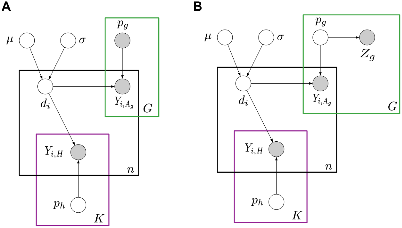
(a) The KP (known population) model, with probe group sizes assumed to be known. (b) The new model, with probe group sizes estimated from respondent reports.

KP Model for Probe Groups Whose Size Is Known

The KP model can be described in three parts. First, we model the size of respondent $i$ ’s personal network, $d_{i}$ , using a log-normal distribution; this approach is similar to previous aggregate relational data models (Maltiel et al. 2015; McCormick et al. 2010; Zheng et al. 2006):

\begin{matrix} μ ~ Uniform (1, 8) \\ σ ~ Uniform (0.25, 2) \\ d_{i} | μ, σ ~ Log - Normal (μ, σ), \end{matrix}

where $μ$ is the mean degree (on the log scale) and $σ$ is the standard deviation in degree (on the log scale).²

Next, the number of reported connections to each probe group is modeled as a function of the probe group size and the respondent’s degree:

\begin{matrix} y_{i, A_{g}} | d_{i}, p_{g} ~ Poisson (d_{i} p_{g}), \end{matrix}

where $y_{i, A_{g}}$ is the number of connections respondent $i$ reports to probe group $A_{g}$ ; $p_{g}$ is the prevalence of probe group $A_{g}$ ; $g$ ranges from $1$ to $G$ ; and $G$ is the total number of probe groups.

Finally, when the goal is to estimate the size of one or more hidden populations, in addition to personal network size, the model has a third component. Reported connections to hidden population $h$ can be modeled as

\begin{matrix} p_{h} ~ Uniform (0, 1) \\ Y_{i, h} | d_{i}, p_{h} ~ Poisson (d_{i} p_{h}), \end{matrix}

where $p_{h}$ is the prevalence of the hidden population. Thus, reported connections to the hidden population are modeled in the same way as reported connections to the probe groups, except information about respondent’s membership in the hidden population is not used.

Incorporating Unknown Probe Group Sizes

To adapt this model-based approach to situations in which the size of the probe groups is not known, we propose modeling the total number of survey respondents who report being members of probe group $g$ , $Z_{g} = \sum_{i \in s} z_{i, g}$ , as a function of the size of the sample, $n = | s |$ , and the population prevalence of probe group, $p_{g}$ :

\begin{matrix} p_{g} ~ Uniform (0, 1) \\ Z_{g} | p_{g}, n ~ Binomial (n, p_{g}) . \end{matrix}

We adopt an uninformative $Uniform (0, 1)$ prior for $p_{g}$ .

This model appears to work well in our empirical examples in the following sections; however, we emphasize that our goal here is keep the model relatively simple by adding just enough complexity to illustrate how estimating the size of the probe groups could be incorporated into a model-based framework. Future work could make this model more elaborate by accounting for possible overdispersion in reported connections to each group and by using a model-based adjustment for errors in recalling reported connections to each group (Maltiel et al. 2015; McCormick et al. 2010; Zheng et al. 2006).

Simulation Study

We created a simulation study as the first empirical test of the estimators proposed above. The goal of the simulation study is to investigate the sampling properties of our new estimators and the previous estimators in controlled environments where the true population values are known. We study the properties of both the design- and model-based degree estimators.

To conduct our simulation study, we start with the Facebook100 (fb100) data set, which is a collection of complete Facebook friendship relationships recorded from the first 100 schools to participate in the social network Facebook (Traud, Mucha, and Porter 2012).³ The fb100 data set is useful because (1) it contains 100 different networks, allowing us to explore a range of real-world patterns of connectivity without resorting to a hypothetical model of network structure, and (2) in addition to network structure, it contains information about several characteristics for each person in the 100 school populations. We use these characteristics to explore the effect of choosing different types of probe groups.

Specifically, for each school, we create candidate probe groups out of the following characteristics: status (distinguishes students, staff members, and faculty members), gender, year, dorm, and major. We treat these characteristics as categorical variables, and we convert each level of each categorical variable (including missingness) into an indicator. For example, there is an indicator variable for whether each person in the school network is a student, an indicator variable for whether each person in the school network is a faculty member, and so forth. We then make a list of all the indicator variables whose prevalence is between 0.1 percent and 10 percent of the population of the school’s network.⁴ We call the groups that satisfy this size requirement the candidate probe groups for each school. Table 1 summarizes these candidate probe groups across all 100 schools. In our simulation study, we investigate many combinations of candidate groups to ensure our results are not overly dependent on one randomly selected candidate group.

Table 1.

Characteristics of the 100 School Networks in Our Sample (N = 100 Schools)

School Characteristic	Median (25th Percentile, 75th Percentile)
Number of people in network	9,950 (4,444, 17,033)
Number of available traits	182 (132, 230)
Number of candidate probe groups	42 (38, 47)
Average candidate group prevalence	.028 (.025, .033)

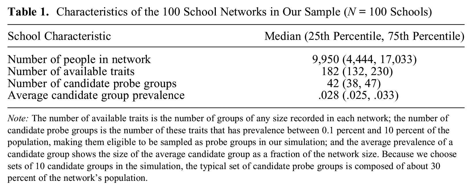
Note: The number of available traits is the number of groups of any size recorded in each network; the number of candidate probe groups is the number of these traits that has prevalence between 0.1 percent and 10 percent of the population, making them eligible to be sampled as probe groups in our simulation; and the average prevalence of a candidate group shows the size of the average candidate group as a fraction of the network size. Because we choose sets of 10 candidate groups in the simulation, the typical set of candidate probe groups is composed of about 30 percent of the network’s population.

In each of the 100 networks in the fb100 data set, we choose $G = 20$ different sets of candidate groups, with each set of candidate groups having a random subset of $10$ of the possible probe groups for the school. We simulate $M = 250$ surveys using each of the possible sets of candidate groups, meaning we simulate a total of $100 \times 20 \times 250 = 500, 000$ surveys. Each simulated survey has a sample size of $N = 500$ .

For each school, the simulation proceeds as follows:

For $g$ in $1, \dots, G = 20$ :

– Draw a set of probe groups A_g by randomly selecting 10 groups from the set of candidate probe groups for the school.

– For $m$ in $1, \dots, M = 250$ :

Simulate a survey sample by choosing a simple random sample (without replacement) of size $N = 500$ people from the school network.

Simulate questions about whether each respondent is a member of each of the 10 groups in A_g.

Simulate aggregate relational data questions (i.e., questions about network connections to members of each of the 10 groups in A_g).

To produce consistent and essentially unbiased estimates of average personal network size, the set of probe groups must satisfy the probe group condition (see part A of the online supplement); this condition says the average network size of probe group members should be the same as the average network size in the population. Note that, according to the design of this simulation, there is no guarantee the probe groups will satisfy the probe group condition; instead, the simulation mimics the reality most researchers face: they must try to pick probe groups without knowing for sure whether the probe group condition is satisfied. Finally, note that taking a simple random sample produces design weights that are equal for all respondents in each simulated survey.

Simulation Results

We first investigate the design-based estimator. For each simulated survey, we calculated two estimates for the average network size: one based on the known population method (which uses information about the size of probe groups; equation 1) and one based on our new estimator (which does not; equation 2). We summarize the accuracy of each estimate by calculating its relative error:

rel - err (\hat{\bar{d}}) = \frac{\hat{\bar{d}} - \bar{d}}{\bar{d}},

(5)

where $\hat{\bar{d}}$ is an estimate for the average network size, and $\bar{d}$ is the true average network size. The relative error will be close to zero when the estimate is accurate, and it will be far from zero when it is inaccurate.

The left-hand panel of Figure 2 and Table 2 compare the distribution of relative errors across all 500,000 simulated surveys for the known population method and for the new estimator. Two findings emerge from the figure: first, the distributions of relative errors from both methods appear to be centered around 0; second, the distribution of relative errors from the known population method is more tightly concentrated around zero than the distribution of relative errors from the new method. Table 2 confirms these observations using quantitative summaries of the two distributions of relative errors shown in the left-hand panel of Figure 2. The table reveals that the average of the relative errors is very close to zero in both cases, suggesting that both estimators have little to no bias. However, the standard deviation of the relative errors, which captures sampling variation, is slightly larger for the new estimator. This is to be expected: because the new method is based on estimating an additional quantity (i.e., the size of the probe groups), it has additional sampling variance (see part B of the online supplement).

Figure 2.

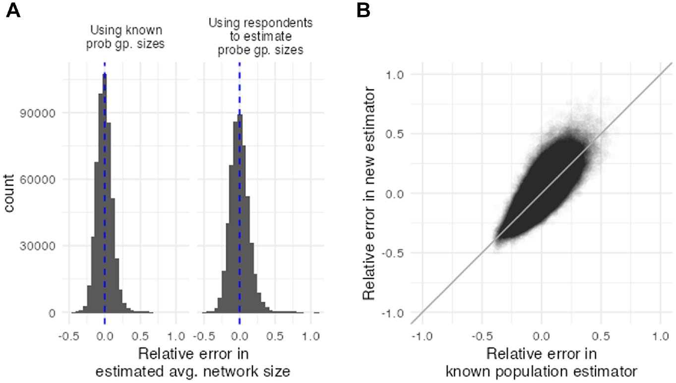
(a) The distribution of relative errors in estimated average network size for the known population method (left) and for the new estimator (right). (b) Comparison of the relative error in estimated average network size using the known population estimator (x-axis) and the new estimator (y-axis).

Table 2.

Mean and Standard Deviation in the Relative Error across All Simulations for Estimating the Average Network Size Using the Known Population Estimator and the New Estimator (Equation 2)

Estimator	Mean (Relative Error)	SD (Relative Error)
Known population (design based)	–.01	.10
New (design based)	.00	.12

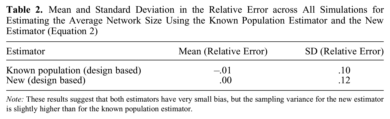
Note: These results suggest that both estimators have very small bias, but the sampling variance for the new estimator is slightly higher than for the known population estimator.

The right-hand panel of Figure 2 shows the relationship between the relative errors for each method; each point in the scatterplot shows the result from one of the 500,000 simulated surveys. The figure shows the relative errors are highly correlated (the correlation coefficient is $ρ = 0.78$ ), meaning that, for a given set of probe groups and a given sample, the known population estimator and the new estimator produce errors that tend to be in the same direction and tend to have the same magnitude.

Next, we investigate model-based estimates for the average network size from the same simulations. The computational burden required to fit the model for every survey we simulated was prohibitive; therefore, we fit the model to a subset of 10 simulated surveys from each of the 100 universities in our sample. The results shown here summarize these 1,000 model fits. 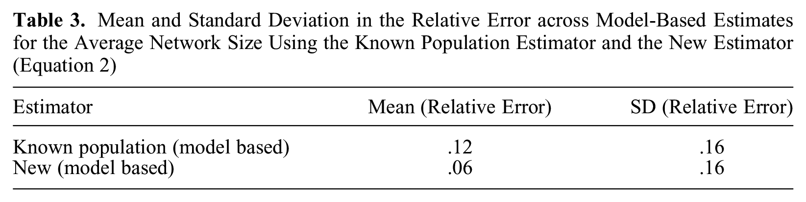We evaluate the model-based point estimates by using the median of the posterior distribution for the estimated average of the degree distribution; in other words, we take as our estimator for $\bar{d}$ the posterior median of the parameter $μ$ in the models above.

Parallel to the results for the design-based estimators, we investigate the relative errors of the model-based fits for (1) the KP model, which requires information about probe group sizes (Figure 1a), and (2) the new model, which estimates the size of the probe groups (Figure 1b). The left-hand panel of Figure 3 shows the distribution of relative errors for the KP model and for the new model. The distributions look qualitatively similar, with both showing evidence of a slight positive bias. This finding is confirmed by Table 3, which reveals that the KP estimator has a moderate positive bias, although with a lot of sample to sample variation. Again, these results are not surprising: model-based estimates would be expected to be unbiased on data generated by the model, but not necessarily on data from a real-world network. The table also suggests that estimating the probe group size from the respondents may slightly reduce the bias, although the sample to sample variation is again considerable. The right-hand panel of Figure 3 compares the relative error for the KP model to the relative error for the new model. 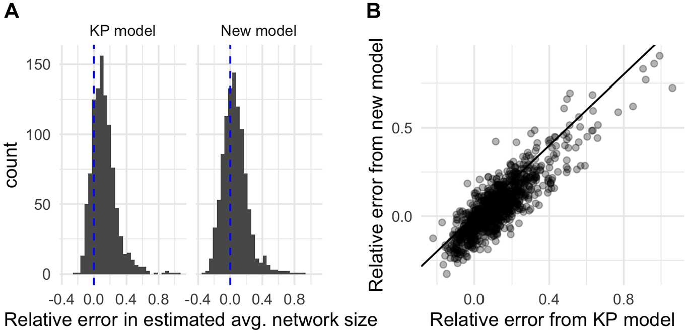Similar to the design-based estimators, there is a high correlation between these two sets of relative errors ( $ρ = 0.86$ ), and the slight reduction in bias from the new model’s estimates is revealed by the fact that points are shifted downward from the diagonal $y = x$ line.

Figure 3.

(a) The distribution of relative errors in estimated average network size for the model with probe group sizes assumed known (left) and with probe group sizes simultaneously estimated (right). (b) Comparison of the relative error in estimated average network size using the model with probe group sizes assumed known (x-axis) and the model with probe group sizes simultaneously estimated (y-axis).

Table 3.

Mean and Standard Deviation in the Relative Error across Model-Based Estimates for the Average Network Size Using the Known Population Estimator and the New Estimator (Equation 2)

Estimator	Mean (Relative Error)	SD (Relative Error)
Known population (model based)	.12	.16
New (model based)	.06	.16

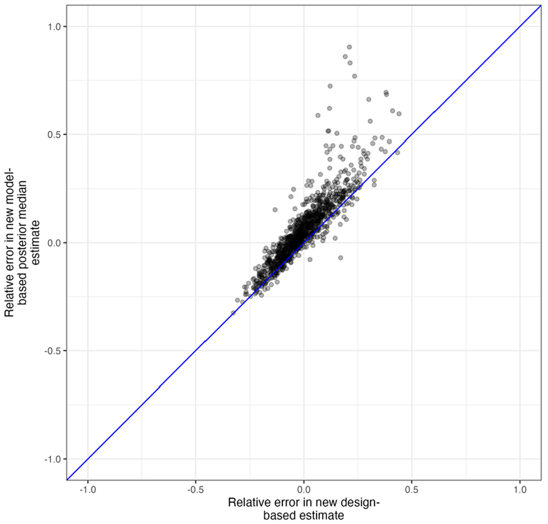
Finally, we assess how similar relative errors from the new design-based estimator are to relative errors from the new model-based estimator. Figure 4 shows the relationship between the relative error in the design-based estimate and the relative error in the model-based posterior median estimate for $μ$ across the 1,000 surveys in our subsample. On average, relative errors from the model-based estimator are about 0.06 higher than relative errors from the design-based estimator, and the correlation coefficient is $ρ = 0.89$ . These findings suggest that, in a given survey, the accuracy of the estimate from the new design-based estimator is quite similar to the accuracy of the estimate from the new model-based estimator.

Figure 4.

Comparison between relative error in the design-based estimate (x-axis) and the model-based estimate (y-axis) for the subsample of 1,000 simulated surveys we fit the model to.

To wrap up, the simulation study shows that our proposed change in data collection requires relatively simple modifications to both design-based and model-based approaches to estimating average personal network size. In the case of design-based estimators, our simulation results suggest that estimating probe group size from respondents adds a modest amount of sampling variation to the estimates. For model-based estimators, our simulation results suggest there is not a cost, and there may even be modest benefits to estimating probe group sizes from respondents.

Household Survey in Hanoi, Vietnam

The simulation study discussed in the prior section helps illustrate the behavior of our proposed data collection strategy and our new estimators in networks in which the true average network size is known. Of course, this simulation cannot provide direct evidence about how well our proposed methods work in a real-world survey. Thus, we now turn to our second empirical illustration: a household survey we conducted in Hanoi, Vietnam. The goal of the survey was to use the network scale-up method to estimate the size of four hidden populations at elevated risk for HIV/AIDS: female sex workers, men who have sex with men, people who use drugs, and people who inject drugs. For our purposes, this study serves as a field test of estimating probe group size from survey respondents’ reported membership in the probe groups. This survey also allows us to illustrate how design- and model-based scale-up estimators—which aim to use aggregate relational data to estimate the size of a hidden population, rather than just the average network size—can be adapted when probe group sizes are estimated from the sample.

A secondary goal of the survey was to investigate the quantity/quality trade-off, which is hypothesized to be at play when asking respondents to report about people they are connected to through network ties of varying strength (Feehan et al. 2016). When moving from estimates based on a weak-tie definition to estimates based on a stronger tie definition, the quantity/quality hypothesis predicts that two important things will happen. First, because weak-tie networks tend to be bigger than strong-tie networks, we expect to learn about fewer people through strong-tie networks; thus, sampling error should increase when estimates are based on strong-tie networks compared with weak-tie networks. Second, because we expect people to have more accurate information about others whom they are connected to through strong ties, we expect nonsampling errors will decrease in strong-tie networks, compared with weak-tie networks.

Previous empirical work has found support for the quantity/quality trade-off hypothesis when survey respondents report about groups that are not expected to be stigmatized (Feehan and Cobb 2019; Feehan et al. 2016). In our survey, we wished to investigate what effect tie strength might have on reports about potentially stigmatized groups. Thus, our survey asked each respondent questions about their connections to probe groups under four different tie definitions (see Table 4). These tie definitions were designed to be nested inside of one another and to lie on a continuum from very weak ties (any people the respondent knows at all) to relatively strong ties (people the respondent shared a meal with in the past month).

Table 4.

Tie Definitions Used in the Hanoi Survey

Tie Name	Wording
Any	How many taxi drivers do you KNOW who are age 18-54; who currently live in Hanoi; who you know by sight AND name; and who also know you by sight and name? (Note: You should not consider famous people that you know about, but who do not know about you.)
Interaction	How many taxi drivers have you interacted with—through face-to-face conversation, chat, SMS, or email—in the past 12 months?
Meal 12mo	Among [Interaction alters], how many did you share a meal or drink (coffee, tea, beer, etc.) with in the last 12 months?
Meal 1mo	Among [Meal 12mo alters], how many did you share a meal or drink with in the last month?

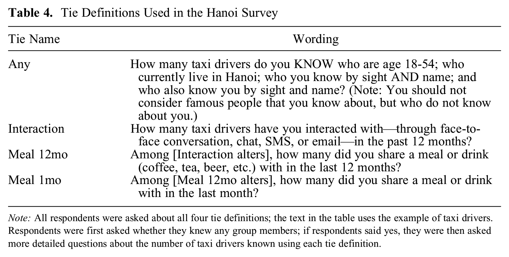
Note: All respondents were asked about all four tie definitions; the text in the table uses the example of taxi drivers. Respondents were first asked whether they knew any group members; if respondents said yes, they were then asked more detailed questions about the number of taxi drivers known using each tie definition.

Probe Groups

Our new approach to data collection gave us great flexibility in considering different types of probe groups for our study. After pilot-testing several different possibilities, we decided to use occupations as our probe groups (see Table 5). Importantly, we were able to focus on how effectively respondents would be able to understand and reply to questions about the probe groups, rather than being constrained to groups whose totals existed in administrative records. For example, motorcycle taxis called xe om are common in Hanoi. It is clear to people in Hanoi who xe om drivers are, so they could answer a survey question about how many xe om drivers they were connected to. But we were not able to locate any administrative data about the total number of xe om drivers in the city. Even if some administrative data existed, official tallies might not include xe om drivers in the informal sector. So it would not have been possible to use xe om drivers as a probe group in conjunction with the known population method. Our approach enabled us to use xe om drivers as a probe group despite the lack of administrative information: by asking survey respondents if they are themselves xe om drivers, we can estimate the total number of xe om drivers in Hanoi from our probability sample.

Table 5.

Probe Groups Used in the Hanoi Survey

Probe Group
Doctor
Lawyer
Primary teacher
Bank worker
Taxi driver
Xe om driver
Hairdresser
Nurse
Coffee shop owner
Farmer (rice grower only)
Builder/mason
Security guard
Student

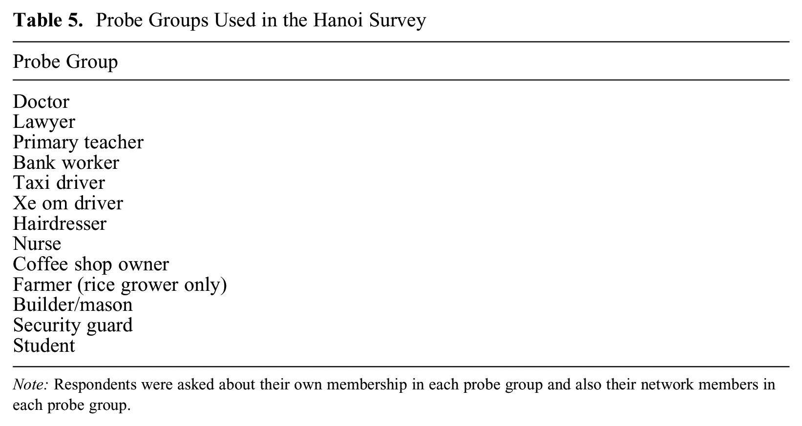
Note: Respondents were asked about their own membership in each probe group and also their network members in each probe group.

Estimating probe group sizes from the survey allowed us to circumvent similar challenges for several other occupations, for which we also found no Hanoi-specific administrative data. Previous experience designing network scale-up studies suggests this situation is not unusual: it can be difficult to get accurate administrative data about the number of people in different occupations, particularly for a specific geographic area and for occupations that are often largely informal. Even when administrative data can be located, it can be difficult to ascertain how complete and accurate they are.

Results

We partnered with Vietnam’s national statistical agency, GSO, to obtain a probability sample of households in Hanoi as part of the Vietnam Health and Living Standards (VHLS) survey. The VHLS was collected using a complex, multistage design that produced a representative sample of adults living in Hanoi. We obtained our sample of $n = 595$ respondents from a randomly selected subset of the households interviewed as part of VHLS in Hanoi. To account for the complex sampling design, all of the design-based analyses use the sampling weights, and sampling uncertainty is estimated using the rescaled bootstrap (Feehan and Salganik 2016b; Rao and Wu 1988; Rao, Wu, and Yue 1992). Our model-based estimates do not use the sampling weights, which is consistent with previous studies that use the model-based approach in this context (e.g., Killworth, McCarty, et al. 1998; Maltiel et al. 2015; McCormick et al. 2010; Zheng et al. 2006). Part E of the online supplement provides additional information about the sampling design.

Our survey instrument had three parts. First, each respondent was asked some basic demographic questions, including whether they were personally a member of any of the occupational groups listed in Table 5.⁵ Responses to these survey questions enable us to estimate the size of the probe groups. Next, each survey respondent was asked questions about their connections to people in the probe groups through each of the four network ties. Responses to these questions allowed us to estimate the average network size of each respondent in each of the four networks using the design-based estimator (equation 2) and the model (Figure 1). Finally, each survey respondent was asked additional aggregate relational data questions about hidden populations whose size we wished to estimate. Again, we use responses to these questions together with the adapted design-based scale-up estimator (equation 4) and the adapted model-based estimator (Figure 1) to produce two sets of estimated hidden population sizes.

About 26 percent of respondents reported being a member of one of the probe groups.⁶ Figure 5 shows the resulting size estimates. Several of the probe groups are estimated to be quite small, around 10,000 to 20,000 people. But these small groups do not necessarily pose a problem for the estimators: the denominator of the design-based estimator (equation 2) reveals that estimating the size of respondents’ personal networks requires the total probe group size, and not the size of each individual probe group. Figure 5 shows this quantity is estimated to be much larger, approximately a fifth of the adult population in Hanoi.

Figure 5.

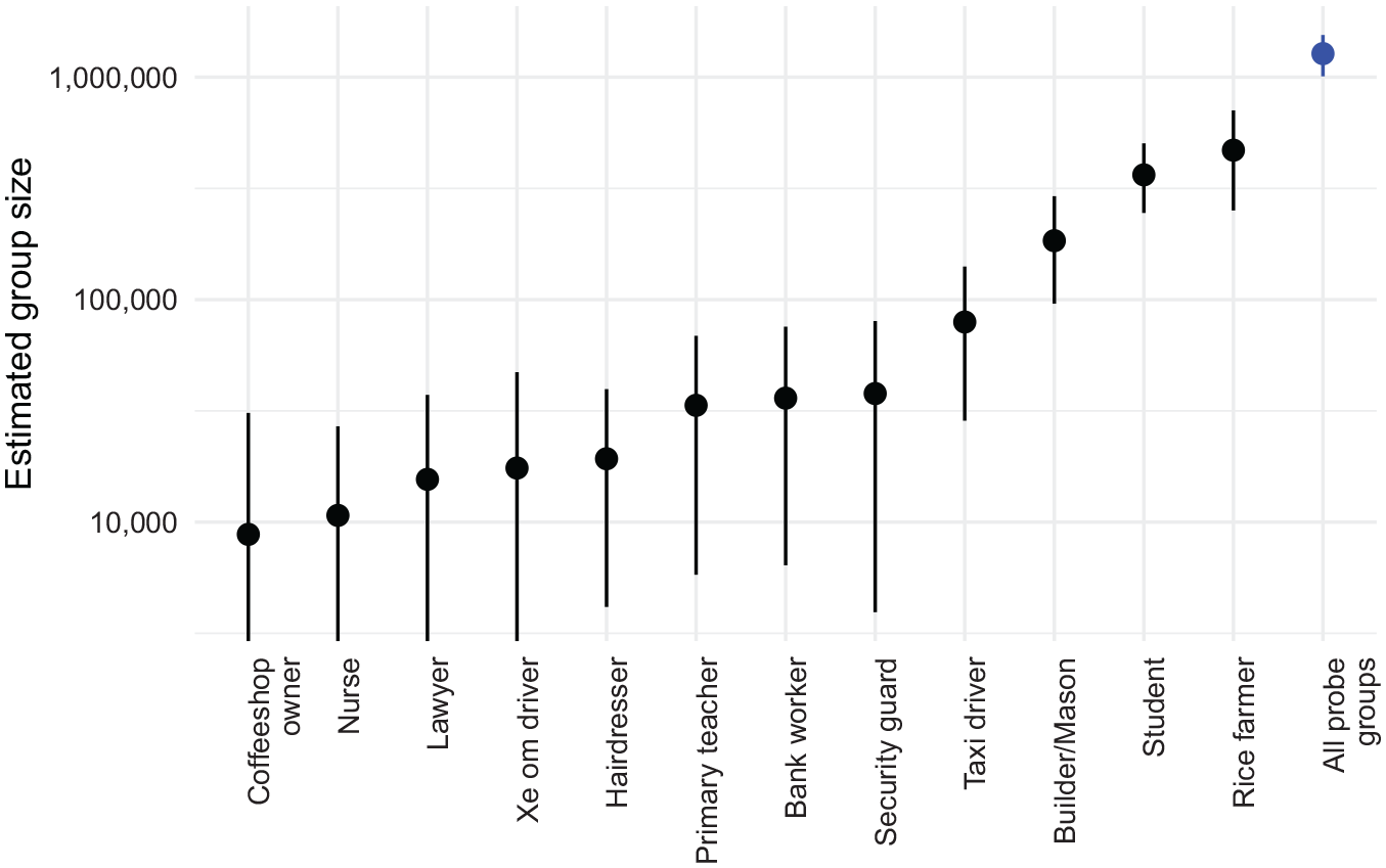
Estimated size of each probe group population and estimated total size of all probe group populations (in blue).

After reporting about their own membership in the probe groups, respondents were asked how many connections they had to each probe group using each of the four tie definitions shown in Table 4. Figure 6 summarizes the responses by showing the average number of reported connections for each probe group and for each tie definition. (Note that the y-axis of the figure is on a log scale.) Two important features emerge from Figure 6. First, for all groups, the average number of reported contacts decreases as tie definitions move from weaker to stronger. This is consistent with what we would expect from the design of the tie definitions, and from the way questions were asked in the survey: respondents first reported “any contact” and were then asked about each of the stronger tie definitions in turn. Second, the order of probe groups is quite stable across tie definitions: for each pair of tie definitions, we calculated the rank correlation coefficient between the average number of reported connections to each probe group; the smallest of these correlation coefficients was 0.89. Thus, groups that have relatively large numbers of reported connections for one tie tend to have relatively large numbers of reported contacts for another.

Figure 6.

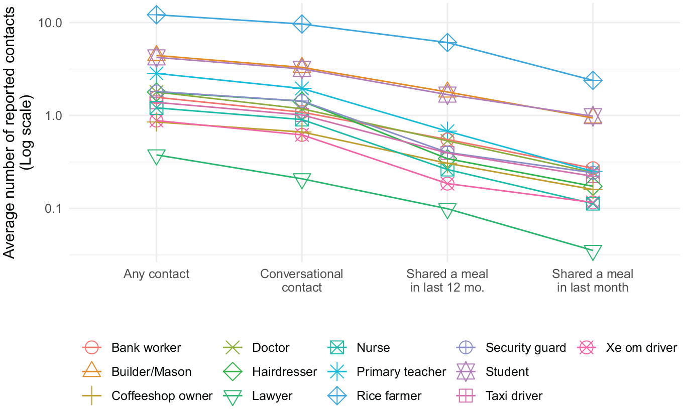
Average number of reported connections to each probe group for each of the four network ties used in the Hanoi survey.

Figure 7 shows the estimated average network size among adult residents of Hanoi for each tie definition using the design-based and model-based estimators. These estimated network sizes are based on combining the information shown in Figures 5 and 6 using the design-based (red) and model-based (blue) estimators. The design-based estimates have 95 percent confidence intervals, which capture sampling uncertainty and were calculated using the rescaled bootstrap (Feehan and Salganik 2016b; Rao and Wu 1988; Rao et al. 1992). Model-based estimates are 95 percent credible intervals based on MCMC draws from the model posterior. Three salient features emerge from Figure 7. First, as expected, estimated average network size decreases as the tie definition becomes stronger. Second, the estimated average personal network sizes from the design-based estimator are very similar to the estimated average personal network sizes from the model-based estimator. This was somewhat surprising: it was not obvious, ex ante, that the two estimates would agree. The design-based estimate uses the sampling weights, together with the relatively simple estimator in equation 2; the model-based estimator, on the other hand, requires more complexity to estimate, and it disregards the sampling weights altogether. Third, the estimated uncertainty in each set of estimates is also quite similar between the two methods. Again, it was not obvious this would be the case: the design-based intervals show an estimate of the sampling variance, incorporating the sampling weights and the sampling design, whereas the model-based intervals show uncertainty estimated using the stochastic assumptions encoded in the model.

Figure 7.

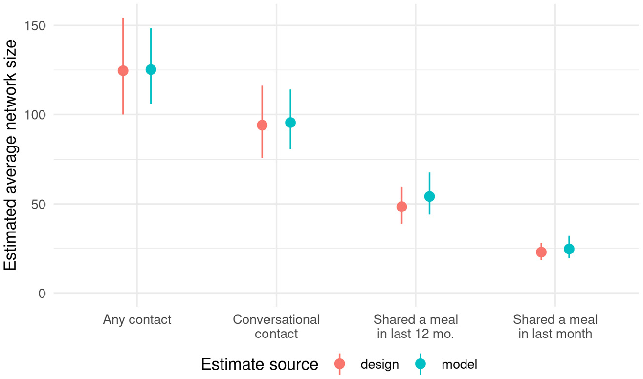
Estimated average personal network size of adult residents of Hanoi, Vietnam.

At the end of the survey, respondents were asked about their connections to four hidden populations that are at elevated risk for HIV/AIDS: female sex workers, men who have sex with men, people who inject drugs, and people who use drugs. These questions were framed in the same way as the questions about connections to the probe groups; however, rather than reporting their responses to the interviewer, respondents were asked to self-administer the responses to these more sensitive questions using a separate form. (These groups are socially stigmatized in many populations, and the goal was to try to mitigate the effects of social desirability bias; for more detail, see part F of the online supplement.) We also wanted to compare patterns of reported connections to the potentially stigmatized hidden populations to patterns of connections to groups we did not expect to be stigmatized. Thus, as part of the self-administered questionnaire, respondents were asked to report their connections to two additional groups: women who smoke and women who had babies in the past 12 months.

Figure 8 shows the estimated size of each group using the model-based and design-based estimators. Again, design-based estimates are shown with 95 percent confidence intervals, which capture sampling uncertainty and were calculated using the rescaled bootstrap (Feehan and Salganik 2016b; Rao and Wu 1988; Rao et al. 1992). Model-based estimates have 95 percent credible intervals based on Markov-chain Monte Carlo draws from the model posterior.

Figure 8.

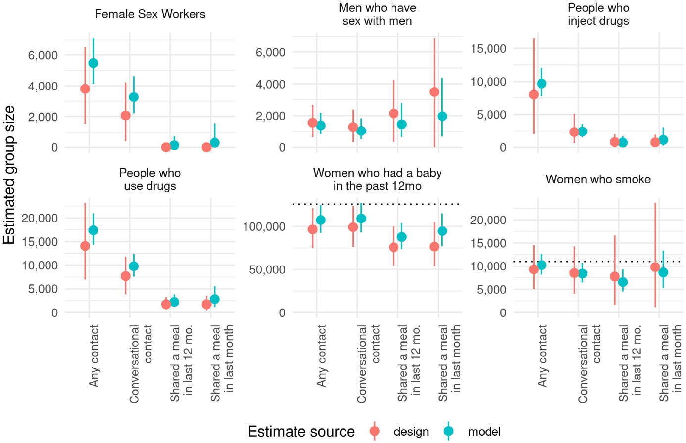
Network scale-up estimates for the size of four hidden populations (female sex workers, men who have sex with men, people who inject drugs, and people who use drugs), and two other populations (women who smoke and women who had babies in the past 12 months).

We use differences in size estimates across the four different network ties shown in Figure 8 to assess the predictions of the quantity/quality trade-off hypothesis. The results in Figure 8 are generally consistent with the first prediction of the quantity/quality trade-off hypothesis: in these estimates, the relative sampling error increases as the tie definition gets stronger (see Table 10 in the online supplement). However, Figure 8 shows that support for the second prediction, that nonsampling error decreases as tie definition gets stronger, is less clear. For one group, men who have sex with men, we see modest increases in estimated size as the tie definition gets stronger. As discussed in part F of the online supplement, this pattern is consistent with what we would expect if people are more likely to be aware that their strong-tie network connections are men who have sex with men, which is in turn consistent with the quantity/quality trade-off hypothesis’s prediction that reports from stronger ties will have lower nonsampling error. But for the other three groups—female sex workers, people who inject drugs, and people who use drugs—the highest estimates came from the weakest tie definition. Taking people who use drugs as an example, we can think of three plausible explanations for these patterns: first, when asked to report about connections to these groups, people may be more likely to speculatively include weak-tie connections as drug users; second, people may be more aware that weak-tie connections are drug users because people who use drugs make an effort to hide their status from stronger tie connections; and third, stigma associated with drug use may lead respondents to be unwilling to disclose that close network connections are drug users but more willing to disclose that weaker tie network connections are drug users. In part F of the online supplement, we discuss these possibilities in greater detail. Of course, it is also possible that these factors interact with each other to produce the patterns observed here.

One way to better understand the mechanism behind the cross-tie patterns in size estimates from Figure 8 would be to compare the estimates with high-quality reference data on the size of these hidden populations. Unfortunately, for most groups shown in Figure 8, no high-quality reference estimates were available. However, we were able to find approximate comparison estimates for the groups we did not expect to be stigmatized: women who smoke and women with babies younger than 1 year. We approximate the number of women who had babies younger than 1 year by simply taking GSO’s population projection for people ages 0 to 4 in Hanoi and dividing it by 5; this is roughly the number of babies younger than 1 year, which is in turn roughly the number of women who had babies in the past 12 months. For women who smoke, we were able to obtain point estimates from an epidemiological study that estimated the prevalence of smoking among women in Hanoi. (See part F of the online supplement for more information on how we calculated these comparison estimates.) The horizontal dotted lines in Figure 8 show these alternative estimates in comparison with the scale-up estimates from each tie definition. The scale-up estimates agree well with the approximate comparison for women who smoke and are somewhat lower than the rough number of women who had babies in the past year.

Discussion

We propose a simple change in how aggregate relational data can be collected on a survey: rather than requiring that the size of probe groups be known from administrative records or census data, we show that researchers can estimate the size of probe groups directly from survey respondents. By eliminating the need to find data about probe groups, this change can greatly increase the flexibility of these methods. We show how to adapt existing design- and model-based estimators for network size to use data collected in this way.

To test our new approach in a controlled setting in which true population values were known, we conducted a simulation study. The results of the simulation study suggest estimating the size of probe groups from information about respondents performs well: it appears to add little or no bias. The new approach increases sampling uncertainty a small amount for the design-based estimator, and it may reduce errors a little bit for the model-based estimator.

To test our new approach in the field, we conducted a household survey in Hanoi, Vietnam. We showed how our approach enabled occupations to be used as probe groups, despite the lack of administrative data on the size of each occupational group. We also experimented with asking survey respondents to simultaneously report about more than one different type of network tie. Asking about different ties enabled us to simultaneously estimate the size of several different networks; it also allowed us to use the scale-up method to produce multiple estimates for the size of four hidden populations.

Our results show that asking about ties of different strength can produce informative patterns, and we interpret these cross-tie patterns in size estimates in light of the previously hypothesized quantity/quality trade-off. The results suggest mixed support for the predictions of the quantity/quality trade-off hypothesis: in all cases, sampling error increased as respondents reported about stronger ties. However, we also expected respondents would omit fewer hidden population members from reports about stronger network ties; if this were the case, we would expect to see stronger ties produce larger size estimates for each hidden population. We only find this pattern for one of the groups, men who have sex with men. This suggests that further work is needed to fully understand the trade-offs at play when respondents are asked to report about hidden populations that may be stigmatized. In part F of the online supplement, we develop formal models that can be useful in reasoning about these potential trade-offs.

Our results allow us to update some recommendations for future studies that collect aggregate relational data. First, our findings demonstrate that researchers need not be restricted to probe groups whose size can be found in administrative or census data. We recommend that rather than focusing on probe groups for whom administrative data are available, researchers instead focus on finding (1) probe groups that are most likely to satisfy the probe group condition, that is, probe groups whose members are typical of frame population members, in terms of their average network size, and (2) probe groups that are easy for survey respondents to understand and report about.

Best practices currently suggest that 20 probe groups are needed to effectively estimate personal network size using the known population method (Bernard et al. 2010); in our study, we found a smaller number of probe groups could also work well: we used 10 probe groups in the simulation study and 13 probe groups in the Hanoi survey. Future work could explore which factors are most important in choosing an effective number of probe groups; we expect the optimal number will depend on the tie definition, as well as the size and nature of the probe groups.

Our simulation results showed quite similar performance for the design- and model-based estimators, with the design-based estimators achieving slightly lower errors. We expect that in situations with moderate to large sample sizes and known probabilities of inclusion, the design-based estimator may be simpler and more transparent to use. On the other hand, when sample sizes are small, or when researchers wish to incorporate additional information in the estimation, the model-based estimators may be more appealing. Here, we showed that both approaches can successfully be adapted to work with probe group sizes that are estimated from the survey respondents; we leave a more thorough comparison of these two approaches to future work.

Our study had several important limitations, and these limitations help outline potential directions for future research. In our empirical studies, we used only probe groups whose size was estimated from survey respondents. Future studies could investigate the potential benefits of combining questions about probe groups whose size is known with questions about probe groups whose size is estimated from respondents. This approach could also permit internal consistency checks to be used with our new approach to data collection (see part B of the online supplement for a discussion of this topic).

In the Hanoi survey, we estimated the size of four hidden populations at elevated risk for HIV/AIDS using a scale-up survey alone. Previous research shows that the conditions required by the scale-up estimator can be relaxed if researchers also obtain parallel samples among members of each hidden population (e.g., Feehan and Salganik 2016a; Salganik et al. 2011). These data would be especially valuable here because they could potentially help explain the mechanisms behind the cross-tie pattern of estimates shown in Figure 8. Future studies could combine information from a probability sample of the population with additional samples of members of the hidden population for multiple ties to help provide empirical evidence about possible mechanisms driving differences in tie-specific size estimates.

It would also be valuable to develop study designs to disentangle mechanisms that could lead to the cross-tie patterns we found in our Hanoi study results. Our results suggest different tie definitions can produce different estimates for the size of a hidden population. The context-specific relationship between the tie definition and the hidden population being studied may play an important role in determining which network tie will produce the best size estimate. Future studies could explore novel approaches to empirically quantifying the effect that stigma might have as a function of tie strength; for example, future work might explore incorporating list experiments (e.g., Blair and Imai 2012; Glynn 2013) or randomized response designs (e.g., Warner 1965) to scale-up studies.

In this study, we used a relatively simple model to illustrate how to adapt model-based estimators to our methods. Future work could expand the model to incorporate innovations that have been previously developed in the scale-up literature, such as regression-based adjustments for recall errors (e.g., McCormick et al. 2010) and estimated barrier effects (Maltiel et al. 2015).

In our estimators, both model based and design based, we did not explicitly address the concern of missing data. In the Hanoi survey, there was no missingness on respondents’ membership in the probe groups, and missingness was very low in reported connections to probe groups (see Table 11 in the online supplement). However, we expect that if our methods are applied in other settings, there may be more missingness. Understanding how to best account for this missingness in the analysis is an important direction for future work.

Our survey in Hanoi was conducted on paper, so we do not have precise data on how long each question took to administer. Future work could collect data such as these electronically, for example using tablets. Careful measurements of the time spent on each question would be useful for planning future studies.

Finally, the point estimates from our simulation study and from our field test in Hanoi both revealed that estimates from the model- and design-based approaches were strikingly similar. This was somewhat surprising: the Hanoi study was based on a complex sampling design, and the model-based estimator ignored the survey weights. It would be useful to better understand when the model-based estimators can safely ignore the sampling design and, more generally, how to incorporate survey weights into complex models.

Supplemental Material

sj-pdf-1-smx-10.1177_00811750221109568 – Supplemental material for Survey Methods for Estimating the Size of Weak-Tie Personal Networks

Supplemental material, sj-pdf-1-smx-10.1177_00811750221109568 for Survey Methods for Estimating the Size of Weak-Tie Personal Networks by Dennis M. Feehan, Vo Hai Son and Abu Abdul-Quader in Sociological Methodology

Footnotes

Acknowledgements

We thank Ashton Verdery, Casey Breen, and Jess Kunke for helpful comments on drafts of this manuscript. We are also grateful to Nga Nguyen and Ali Safarnejad of UNAIDS Hanoi for help during data collection and to Hanh Bui of the University of California, Berkeley, for research assistance. D.M.F. thanks the Berkeley Population Center, which is funded by the Eunice Kennedy Shriver National Institute of Child Health and Development (grant P2C HD 073964), and the Berkeley Center for the Economics and Demography of Aging, which is funded by the National Institute on Aging (grant 5P30AG012839). The views and opinions expressed in this paper are those of the authors and not of the organizations or agencies where the authors are employed. Replication code and data are available at

ORCID iD

Dennis M. Feehan

Supplemental Material

Supplemental material for this article is available online.

Notes

Author Biographies

Dennis M. Feehan is an assistant professor in the Department of Demography at the University of California, Berkeley.

Vo Hai Son is a medical doctor, an epidemiologist, and a senior in the Vietnam Authority of HIV/AIDS Control, Ministry of Health.

Abu Abdul-Quader is an epidemiologist with the Division of Global HIV and TB Prevention at the Centers for Disease Control and Prevention in Atlanta, Georgia.

References

Bernard

H. Russell

Hallett

Tim

Iovita

Alexandrina

Johnsen

Eugene C.

Lyerla

Rob

McCarty

Christopher

Mahy

Mary

, et al. 2010. “Counting Hard-to-Count Populations: The Network Scale-Up Method for Public Health.” Sexually Transmitted Infections 86(Suppl. 2):ii11–15.

Bernard

H. Russell

Johnsen

Eugene C.

Killworth

Peter D.

Robinson

Scott

. 1989. “Estimating the Size of an Average Personal Network and of an Event Subpopulation.” Pp. 159–75 in The Small World, edited by Kochen

Norwood, NJ: Ablex.

Blair

Graeme

Imai

Kosuke

. 2012. “A Statistical Analysis of List Experiments.” Political Analysis 20(1):47–77.

Carpenter

Bob

Gelman

Andrew

Hoffman

Matthew D.

Lee

Daniel

Goodrich

Ben

Betancourt

Michael

Brubaker

Marcus

, et al. 2017. “Stan: A Probabilistic Programming Language.” Journal of Statistical Software 76(1).

de Sola Pool

Ithiel

Kochen

Manfred

. 1978. “Contacts and Influence.” Social Networks 1(1):5–51.

Deville

Jean-Claude

Särndal

Carl-Erik

. 1992. “Calibration Estimators in Survey Sampling.” Journal of the American Statistical Association 87(418):376–82.

DiPrete

Thomas A.

Gelman

Andrew

McCormick

Tyler

Teitler

Julien

Zheng

Tian

. 2011. “Segregation in Social Networks Based on Acquaintanceship and Trust.” American Journal of Sociology 116(4):1234–83.

Feehan

Dennis M.

2015. “Network Reporting Methods.” PhD dissertation, Princeton University. Retrieved June 17, 2022. http://gradworks.umi.com/37/29/3729745.html.

Feehan

Dennis M.

Cobb

Curtiss

. 2019. “Using an Online Sample to Estimate the Size of an Offline Population.” Demography 56(6):2377–92.

10.

Feehan

Dennis M.

Salganik

Matthew J.

2016a. “Generalizing the Network Scale-Up Method: A New Estimator for the Size of Hidden Populations.” Sociological Methodology 46(1):153–86.

11.

Feehan

Dennis M.

Salganik

Matthew J.

2016b. “Surveybootstrap: Tools for the Bootstrap with Survey Data.” Retrieved June 17, 2022. https://CRAN.R-project.org/package=surveybootstrap.

12.

Feehan

Dennis M.

Umubyeyi

Aline

Mahy

Mary

Hladik

Wolfgang

Salganik

Matthew J.

2016. “Quantity versus Quality: A Survey Experiment to Improve the Network Scale-Up Method.” American Journal of Epidemiology 183(8):747–57.

13.

Fischer

Claude S.

1982. To Dwell among Friends. Chicago: University of Chicago Press.

14.

Glynn

Adam N.

2013. “What Can We Learn with Statistical Truth Serum? Design and Analysis of the List Experiment.” Public Opinion Quarterly 77(S1):159–72.

15.

Granovetter

Mark S.

1973. “The Strength of Weak Ties.” American Journal of Sociology 78(6):1360–80.

16.

Habecker

Patrick

Dombrowski

Kirk

Khan

Bilal

. 2015. “Improving the Network Scale-Up Estimator: Incorporating Means of Sums, Recursive Back Estimation, and Sampling Weights.” PLoS ONE 10(12):e0143406.

17.

Killworth

Peter D.

Johnsen

Eugene C.

Bernard

H. Russell

Shelley

Gene Ann

McCarty

Christopher

. 1990. “Estimating the Size of Personal Networks.” Social Networks 12(4):289–312.

18.

Killworth

Peter D.

Johnsen

Eugene C.

McCarty

Christopher

Shelley

Gene A.

Russell Bernard

1998. “A Social Network Approach to Estimating Seroprevalence in the United States.” Social Networks 20(1):23–50.

19.

Killworth

Peter D.

McCarty

Christopher

Bernard

H. Russell

Johnsen

Eugene C.

Domini

John

Shelly

Gene A.

2003. “Two Interpretations of Reports of Knowledge of Subpopulation Sizes.” Social Networks 25(2):141–60.

20.

Killworth

Peter D.

McCarty

Christopher

Bernard

H. Russell

Shelley

Gene A.

Johnsen

Eugene C.

1998. “Estimation of Seroprevalence, Rape, and Homelessness in the United States Using a Social Network Approach.” Evaluation Review 22(2):289–308.

21.

Lubbers

Miranda J.

Luis Molina

José

Valenzuela-García

Hugo

. 2019. “When Networks Speak Volumes: Variation in the Size of Broader Acquaintanceship Networks.” Social Networks 56:55–69.

22.

Lumley

Thomas

. 2010. Complex Surveys: A Guide to Analysis Using R. Hoboken, NJ: John Wiley.

23.

Lumley

Thomas

. 2019. “Survey: Analysis of Complex Survey Samples.” Retrieved June 17, 2022. http://r-survey.r-forge.r-project.org/survey/.

24.

Maltiel

Rachael

Raftery

Adrian E.

McCormick

Tyler H.

Baraff

Aaron J.

2015. “Estimating Population Size Using the Network Scale up Method.” Annals of Applied Statistics 9(3):1247–77.

25.

Marsden

Peter V.

2005. “Recent Developments in Network Measurement.” Pp. 8–30 in Models and Methods in Social Network Analysis, edited by Carrington

P. J.

Scott

Wasserman

Cambridge, UK: Cambridge University Press.

26.

McCarty

Chris H.

Bernard

Russell

Killworth

Peter D.

Shelley

Gene A.

Johnsen

Eugene C.

1997. “Eliciting Representative Samples of Personal Networks.” Social Networks 19(4):303–23.

27.

McCarty

Christopher

Killworth

Peter D.

Bernard

H. Russell

Johnsen

Eugene C.

Shelley

Gene A.

2001. “Comparing Two Methods for Estimating Network Size.” Human Organization 60(1):28–39.

28.

McCormick

Tyler H.

Salganik

Matthew J.

Zheng

Tian

. 2010. “How Many People Do You Know? Efficiently Estimating Personal Network Size.”Journal of the American Statistical Association 105(489):59–70 (https://doi.org/10.1198/jasa.2009.ap0851810.1198/jasa.2009.ap08518).

29.

Perry

Brea L.

Pescosolido

Bernice A.

Borgatti

Stephen P.

2018. Egocentric Network Analysis: Foundations, Methods, and Models. Cambridge, UK: Cambridge University Press.

30.

Rao

J.N.K.

Pereira

Norma P.

1968. “On Double Ratio Estimators.” Sankhyā: The Indian Journal of Statistics, Series A 30(1):83–90.

31.

Rao

J.N.K.

C.F.J.

1988. “Resampling Inference with Complex Survey Data.” Journal of the American Statistical Association 83(401):231–41.

32.

Rao

J.N.K.

C.F.J.

Yue

1992. “Some Recent Work on Resampling Methods for Complex Surveys.” Survey Methodology 18(2):209–17.

33.

Salganik

Matthew J.

Mello

Maeve B.

Abdo

Alexandre H.

Bertoni

Neilane

Fazito

Dimitri

Bastos

Francisco I.

2011. “The Game of Contacts: Estimating the Social Visibility of Groups.” Social Networks 33(1):70–78.

34.

Särndal

Carl Erik

Swensson

Bengt

Wretman

Jan

. 2003. Model Assisted Survey Sampling. Berlin, Germany: Springer Verlag.

35.

Sully

Elizabeth

Giorgio

Margaret

Anjur-Dietrich

Selena

. 2020. “Estimating Abortion Incidence Using the Network Scale-up Method.” Demographic Research 43(56):1651–84.

36.

Teo

Alvin Kuo Jing

Prem

Kiesha

Chen

Mark I. C.

Roellin

Adrian

Wong

Mee Lian

Hanh Hao

Cook

Alex R.

2019. “Estimating the Size of Key Populations for HIV in Singapore Using the Network Scale-Up Method.” Sexually Transmitted Infections 95(8):602–607.

37.

Traud

Amanda L.

Mucha

Peter J.

Porter

Mason A.

2012. “Social Structure of Facebook Networks.” Physica A: Statistical Mechanics and Its Applications 391(16):4165–80.

38.

Valliant

Richard

Dever

Jill A.

Kreuter

Frauke

. 2013. Practical Tools for Designing and Weighting Survey Samples. New York: Springer.

39.

Warner

Stanley L.

1965. “Randomized Response: A Survey Technique for Eliminating Evasive Answer Bias.” Journal of the American Statistical Association 60(309):63–69.

40.

Wolter

Kirk

. 2007. Introduction to Variance Estimation. 2nd ed. New York: Springer.

41.

Zheng

Tian

Salganik

Matthew J.

Gelman

Andrew

. 2006. “How Many People Do You Know in Prison? Using Overdispersion in Count Data to Estimate Social Structure in Networks.” Journal of the American Statistical Association 101(474):409–23.

Supplementary Material

Please find the following supplemental material available below.

For Open Access articles published under a Creative Commons License, all supplemental material carries the same license as the article it is associated with.

For non-Open Access articles published, all supplemental material carries a non-exclusive license, and permission requests for re-use of supplemental material or any part of supplemental material shall be sent directly to the copyright owner as specified in the copyright notice associated with the article.

0.00 MB

1.20 MB