Sage Journals: Discover world-class research

Abstract

Panel data analysis is common in the social sciences. Fixed effects models are a favorite among sociologists because they control for unobserved heterogeneity (unexplained variation) among cross-sectional units, but estimates are biased when there is unobserved heterogeneity in the underlying time trends. Two-way fixed effects models adjust for unobserved time heterogeneity but are inefficient, cannot include unit-invariant variables, and eliminate common trends: the portion of variance in a time-varying variable that is invariant across cross-sectional units. This article introduces a general panel model that can include unit-invariant variables, corrects for unobserved time heterogeneity, and provides the effect of common trends while also allowing for unobserved unit heterogeneity, time-varying coefficients, and time-invariant variables. One-way and two-way fixed effects models are shown to be restrictive forms of this general model. Other restrictive forms are also derived that offer all the usual advantages of one-way and two-way fixed effects models but account for unobserved time heterogeneity. The author uses the models to examine the increase in state incarceration rates between 1970 and 2015.

Keywords

panel data fixed effects random effects time heterogeneity mass incarceration

Panel and pooled time-series data are common in the social sciences. Panel data allow researchers to examine temporal change and disentangle causal order (Halaby 2004; Vaisey and Miles 2016). Fixed effects¹ models are an especially popular method for panel data analysis because they control for unobserved heterogeneity (unmeasured variation) among cross-sectional units. Unobserved unit heterogeneity is typically caused by measurement error in a stable unit characteristic or by an omitted time-invariant variable. If an analyst is concerned that some characteristic of the cross-sectional units has gone unmeasured, he or she can control for confounding with a fixed effects model. For this reason, fixed effects is often regarded as the “gold standard” in panel data analysis (Allison 2009; Vaisey and Miles 2016; Wooldridge 2010).

However, fixed effects models assume that there is no unobserved heterogeneity between time periods. Unobserved time heterogeneity can be produced by an unmeasured period effect or because of an unmeasured interaction with time (Bruderl and Ludwig 2015). Two-way fixed effects models that allow for covariance with unmeasured period effects are the dominant approach for addressing time heterogeneity (Imai and Kim forthcoming; Wooldridge 2010), but two-way fixed effects models eliminate common trends: the portion of variance in a time-varying variable that is invariant across cross-sectional units. This is useful in quasi-experimental research designs in which treatment effects cannot produce a common trend (e.g., Angrist and Pischke 2009; Baltagi 2013; Bertrand, Duflo, and Mullainathan 2004), but observational studies often analyze data for which common trends are substantively informative. Common trends typically manifest when cohort effects are sizable (e.g., Yang, Fu, and Land 2004). If there is a universal shift toward for-profit health care in a country, health outcomes are likely to decline in the population at large (Zheng and George 2018). If people tend to consume more crime news media over time, public support for tough crime policies is likely to increase (Enns 2016). In these cases, models that eliminate common trends might misrepresent the sociological relationship of interest.

In this article, I introduce a general panel model that provides the effect of common trends while allowing for covariance with unmeasured period effects. Prior studies have proposed panel models that allow for unobserved unit heterogeneity (Allison 2009; Arellano 1993; Baltagi 2006; Bollen and Brand 2010; Mundlak 1978; Neuhaus and Kalbfleisch 1998), but these models do not address unobserved time heterogeneity. The model introduced here offers a number of important utilities unavailable in other panel models. First, the model provides the effect of common trends, which is not provided by other panel models. Second, the model can include unit-invariant and time-invariant variables, which cannot be included in other models that allow for covariance with unmeasured period effects, such as the two-way fixed effects model. Third, the model allows for time-varying coefficients. Fourth, the two-way fixed effects coefficient is provided by the general model, so the relative advantages of the model come without losing any of the utility of the two-way fixed effects model in terms of causal inference. The model can also be estimated in a multilevel framework and therefore should be familiar to most sociologists and easy to implement in current software.

I begin by introducing terminology and the problem of unobserved time heterogeneity. I then introduce the general model and discusses its relationship to alternative panel models. I derive restrictive forms and discuss estimation and model selection. I next provide an empirical example using state incarceration rates, which shows that substantive conclusions are often affected by model selection. I provide an open-source R package to implement the models.

Modeling Panel Data

Overview and Terminology

Table 1 is a reference table for all notation used in this article. Panel data are represented by repeated observations of cross-sectional units. The pooled panel model is

y_{it} = X_{it}^{'} β + e_{it} .

(1)

where y is a continuous response variable, X is a data matrix of time-varying variables, β is a k vector of coefficients, e is the error, and it is the time-varying observation of cross-sectional unit i at time t for all i = 1, 2, . . ., N and t = 1, 2, . . ., T. We may, for instance, be interested in academic achievement among students. The characteristics of each student are measured repeatedly over time and used to predict their school performance. The coefficients in the pooled model thus represent a blend of the effect of student-level differences, within-student changes, and common trends among students.

Table 1.

Notation and Terminology

Terminology	Notation	Explanation
Units of analysis
Cross-sectional unit or “unit”	i	The unit of analysis to be measured repeatedly across time, for instance, counties, people, or organizations
Time period	t	A particular moment in time, wave, or survey panel
Observation	it	The measurement of each unit at each time period
Input variables
Time-varying variables	X	A matrix of independent variables that vary across time and across units
Time-invariant variables	Z	Variables that vary between units but do not vary over time
Unit-invariant variables	C	Variables that vary between time periods but do not vary between units
Between transformed variables	$\bar{X_{i .}}$	The cross-sectional means, $\bar{X_{i .}} = \frac{\sum_{i} X}{N_{i}}$
Within-transformed variables	$\tilde{X}$	The deviations from the cross-sectional means, $\tilde{X_{it}} = X - \bar{X_{i .}}$
Common trends	$\bar{\bar{X}}$	The time period means of the within variation, $\bar{\bar{X_{. t}}} = \frac{\sum_{t} \tilde{X}}{N_{t}}$
Idiosyncratic transformed variables	$\overset{⌣}{X}$	The deviations from the common trends, ${\overset{⌣}{X}}_{it} = \tilde{X_{it}} - \bar{\bar{X_{it}}}$
Coefficients
Pooled coefficient	$β$	The effect of X on y
Within coefficient	$β^{W}$	The effect of X controlling for all time-invariant variation (the effect of $\tilde{X}$ on $\tilde{y}$ )
Between effect	$β^{B}$	The effect of X controlling for all temporal variation (the effect of $\bar{X_{i .}}$ on $\bar{y_{i .}}$ )
Idiosyncratic effect	$β^{I}$	The effect of X controlling for all unit-invariant variation and all time-invariant variation simultaneously (the effect of $\overset{⌣}{X}$ on $\overset{⌣}{y}$ )
Homogenous-within effect	$β^{HW}$	The effect of common trends (the effect of $\bar{\bar{X}}$ on $\bar{\bar{y}}$ )
Unit fixed effects	$δ$	The coefficients for each unit-specific dummy variable when Z is specified as a matrix of unit-indicator variables
Time fixed effects	$γ$	The coefficients for each time period–specific dummy variable when B is specified as a matrix of time period indicator variables
Error terms
Error	e	The total error in a panel model
Unmeasured between effect	a	The effect of unmeasured time-invariant variables
Unmeasured period effect	$ε$	The effect of unmeasured unit-invariant variables
Idiosyncratic error	u	The random error after removing unmeasured between effects and unmeasured period effects, $u_{it} = e_{it} - a_{i .} - ε_{. t}$
Within error	$ψ$	The error after removing unmeasured between effects, $ψ_{it} = e_{it} - ε_{. t}$

Panel data are distinct from exchangeable data in that there are three sources of variation in the error term:

e_{it} = u_{it} + a_{i .} + ε_{. t},

(2)

where $a_{i .}$ is the unmeasured between effect, $ε_{. t}$ is the unmeasured period effect, and $u_{it}$ is the idiosyncratic error that varies across both time and units. Each component of the error is assumed to have a normal sampling distribution with zero means and normal variance. The unmeasured between effect, for instance, may contain an unmeasured time-invariant student characteristic, such as gender, that influences students’ school performance. The unmeasured period effect $ε_{. t}$ represents the effect of unmeasured unit-invariant variables. For instance, the performance of all students within a school district may decrease over time because of districtwide budget cuts.

The pooled model in equation (1) assumes no unobserved unit heterogeneity. We can relax this assumption using a random effects model:

y_{it} = X_{it}^{'} β + a_{i .} + e_{it} .

(3)

The random effects model allows for an unmeasured between effect but assumes the unmeasured between effect does not correlate with the time-varying variables. For instance, we may assume there are between-student differences in parental education but that these differences in parental education are uncorrelated with the time-varying variables of interest, such as students’ study habits.

When the unmeasured between effect correlates with the time-varying variables, the random effects coefficients are biased and inconsistent (Arellano 1993; Hausman 1978). The most common correction is to control for unmeasured time-invariant characteristics using one-way fixed effects. One-way fixed effects models allow for covariance with unmeasured between effects by controlling for unit-level differences:

y_{it} = X_{it}^{'} β^{W} + Z_{i .}^{'} δ + ψ_{it} .

(4)

$Z_{i .}^{'}$ is a matrix of time-invariant variables, here specified as N– 1 indicator variables for each cross-sectional unit, δ is the N– 1 vector of coefficients representing the effect of each unit, and $ψ_{it}$ is the within-unit error term ( $ψ_{it} = u_{it} + ε_{. t}$ ). $β^{W}$ is the within effect representing the within-unit change in y associated with a within-unit change in X. The inclusion of Z as a matrix of dummy variables absorbs the unmeasured between effect into the unit fixed effect coefficients (δ). Because the within coefficients use only within variation, the model can be reexpressed without the vector of indicator variables by using the within transformation that centers all variables on their cross-sectional means ( ${\tilde{y}}_{it} = y_{it} - {\bar{y}}_{i .}$ ):

{\tilde{y}}_{it} = {\tilde{X}}_{it}^{'} β^{W} + ψ_{it} .

(5)

Fixed effects is unbiased and consistent when X correlates with an unmeasured between effect, but the model is inefficient because it eliminates all time-invariant variation. We could not, for instance, use one-way fixed effects to evaluate how gender influences students’ school performance. Mundlak (1978) introduced a model that allows for time-invariant variables while also allowing for covariance with unmeasured between effects. We can stack the model in equation (5) with a model for the between effects, ${\bar{y}}_{i .} = {\bar{X}}_{i .}^{'} β^{B} + a_{i .}$ , where ${\bar{X}}_{i .}$ are the cross-sectional means for X and $β^{B}$ is the between effect of ${\bar{X}}_{i .}$ on ${\bar{y}}_{i .}$ Combining equation (5) with the model for the between effects gives the between-within model (Arellano 1993; Baltagi 2006):

y_{it} = {\tilde{X}}_{it}^{'} β^{W} + {\bar{X}}_{i .}^{'} β^{B} + a_{i .} + ψ_{it} .

(6)

In balanced panel data, the within effects are equivalent to the estimates obtained from one-way fixed effects. But the model also provides the between effects and can include time-invariant variables. Using the model in equation (6), we could examine the effects of time-invariant variables like gender, as well as the within effect of time-varying variables, such as the effect of within-student changes in study habits on within-student changes in school performance.

Dealing with Time Heterogeneity

The one-way fixed effects model and the between-within model allow for covariance with unmeasured between effects, but both models assume there is no unobserved time heterogeneity (Halaby 2004:532–35; Morgan and Winship 2007:262–71; Wooldridge 2010:269).² This assumption is violated when an unmeasured period effect influences time trends for all units. In our example of school performance, for instance, if districtwide budget cuts decreased students’ school performance but were not included in our model, the within coefficients from our one-way fixed effects model of students’ school performance would be biased and inconsistent.

Two-way fixed effects models are the most widely used model for addressing unobserved time heterogeneity. They allow for covariance with unmeasured period effects by including indicator variables for both cross-sectional units and time periods. Let C be a matrix containing unit-invariant variables, here specified to be indicator variables for each time period, and $γ$ be the “fixed effect” coefficients for each time period. We write the two-way fixed effects model as a function of the within-transformed variables³:

{\tilde{y}}_{it} = {\tilde{X}}_{it}^{'} β^{I} + C_{. t}^{'} γ + u_{it} .

(7)

$β^{I}$ replaces $β^{W}$ because all unit-invariant and time-invariant variation is controlled (i.e., $ε_{. t} = 0$ and $a_{i .} = 0$ ). Because the coefficient only uses the idiosyncratic variation, I refer to $β^{I}$ as the “idiosyncratic” effect. The inclusion of the time indicator variables means that the model is unbiased and consistent even when there is an unmeasured period effect. However, the model is inefficient and cannot include time-invariant or unit-invariant variables. We could not use two-way fixed effects to evaluate the effect of districtwide budget cuts on students’ school performance.

Sources of Time Heterogeneity and Problems with Corrections

In addition to the inability to include unit-invariant variables, there are two primary issues with the two-way fixed effects correction for unobserved time heterogeneity. First, two-way fixed effects models eliminate common trending. Common trending is informative when all units shift in a similar direction over time. We may want to know, for instance, whether the decrease in the national crime rate during the 1990s was driven partly by an increase in antiviolence organizations in major cities (Sharkey, Torrats-Espinosa, and Takyar 2017). Because a national decline in crime is plausible only if we expect that there was a strong over-time shift toward anticrime organizations in most major cities, this explanation is one of common trends.

In this example and similar ones in which we expect that the common trend has a sizable effect, the two-way fixed effects model can provide misleading results. To see this, let $β^{HW}$ be the homogenous-within effect of a common trend. Common trends are invariant across units, representing the average within-variation at each time period. Let $\bar{\bar{X_{. t}^{'}}}$ denote the common trend of X obtained by calculating the average value of $\tilde{X}$ at each time period and ${\bar{\bar{y}}}_{. t}$ be the common trend for y. The model for the common trends is

{\bar{\bar{y}}}_{. t} = \bar{\bar{X_{. t}^{'}}} β^{HW} + ε_{. t} .

(8)

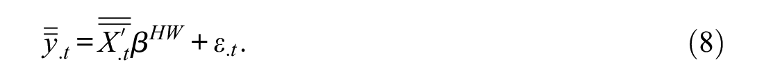
Because the common trend represents a portion of the within variation, we can regard the model in equation (8) as an implied component of the one-way fixed effects model. In two-way fixed effects, however, we aim to set the unmeasured period effect to 0 by replacing $ε_{. t}$ with $C_{. t}^{'} γ$ . As a result, two-way fixed effects overidentifies the model in equation (8).

The second issue is that two-way fixed effects coefficients are biased if there is an unmeasured interaction with time. To correct this, researchers often include interactions between a variable of interest and the time period. This approach, however, grows increasingly inefficient as the number of time periods increases, because each interaction decreases degrees of freedom. Interpretation can also easily become complicated as the number of time periods increases (e.g., Tian et al. 2014). And including many interactions, as is the case in large-T studies, without adjustment produces downwardly biased standard errors (Green and Kern 2012).

Depending on how much variation exists in the common trends, the coefficients provided by two-way fixed effects models may be misleading. If we have a quasi-experimental design in which the primary goal is identification, two-way fixed effects is appropriate because a treatment cannot produce common trends among treated and untreated groups (Angrist and Pischke 2009; Bertrand et al. 2004). However, in many observational studies, common trending is produced by a social process that influences all observations equally. In these cases, common trends are not a nuisance to be eliminated, but an important component of the analysis.

A General Panel Model for Unobserved Time Heterogeneity

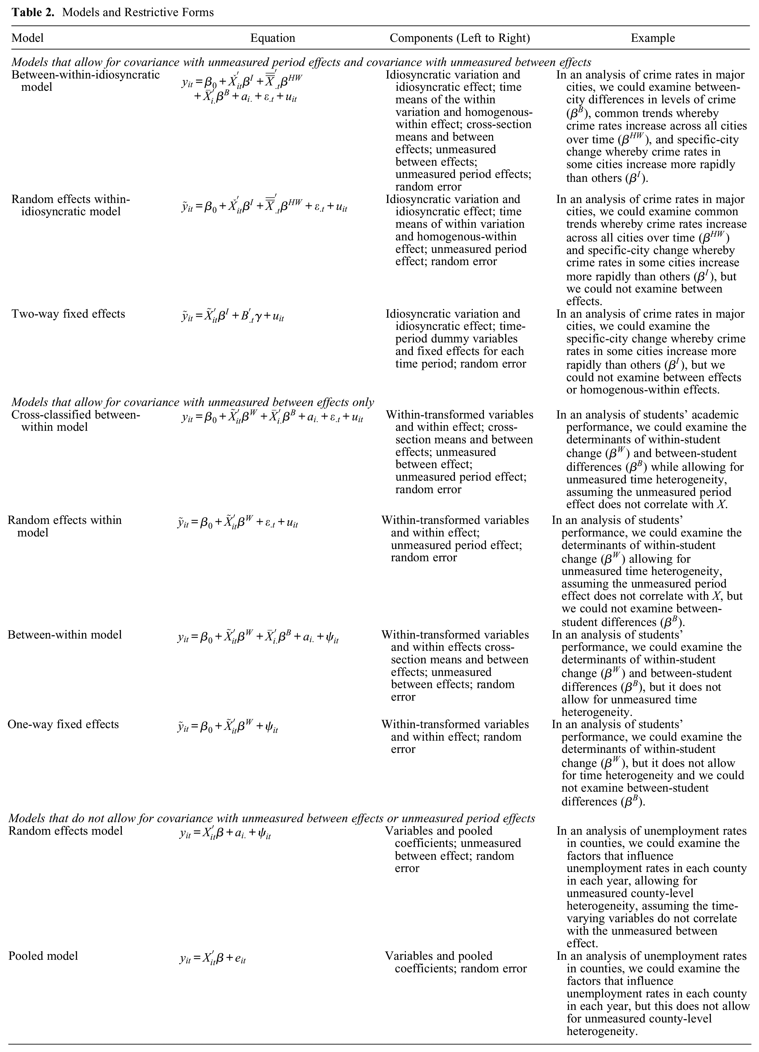
I now introduce a panel model for unobserved time heterogeneity that provides the homogenous-within effect of common trends, the between effect of unit differences, and the idiosyncratic effect usually provided by two-way fixed effects models. The model can also include time-invariant and unit-invariant variables and allows for covariance with unmeasured period effects and unmeasured between effects. I begin by introducing the most general case of the model. The second subsection recasts the model as a multilevel model that allows for time-varying coefficients. The third subsection regards the model as an extension to Bollen and Brand’s (2010) general panel model. The fourth subsection discusses restrictive forms. The remaining subsections are dedicated to estimation, model selection, and exploratory analysis. Table 2 provides the details for each model and hypothetical applications.

Table 2.

Models and Restrictive Forms

Model	Equation	Components (Left to Right)	Example
Models that allow for covariance with unmeasured period effects and covariance with unmeasured between effects
Between-within-idiosyncratic model	$y_{it} = β_{0} + {\overset{⌣}{X}}_{it}^{'} β^{I} + {\bar{\bar{X}}}_{. t}^{'} β^{HW} + {\bar{X}}_{i .}^{'} β^{B} + a_{i .} + ε_{. t}$ + $u_{it}$	Idiosyncratic variation and idiosyncratic effect; time means of the within variation and homogenous-within effect; cross-section means and between effects; unmeasured between effects; unmeasured period effects; random error	In an analysis of crime rates in major cities, we could examine between-city differences in levels of crime ( $β^{B})$ , common trends whereby crime rates increase across all cities over time ( $β^{HW})$ , and specific-city change whereby crime rates in some cities increase more rapidly than others ( $β^{I})$ .
Random effects within-idiosyncratic model	${\tilde{y}}_{it} = β_{0} + {\overset{⌣}{X}}_{it}^{'} β^{I} + {\bar{\bar{X}}}_{. t}^{'} β^{HW} + ε_{. t} + u_{it}$	Idiosyncratic variation and idiosyncratic effect; time means of within variation and homogenous-within effect; unmeasured period effect; random error	In an analysis of crime rates in major cities, we could examine common trends whereby crime rates increase across all cities over time ( $β^{HW})$ and specific-city change whereby crime rates in some cities increase more rapidly than others ( $β^{I})$ , but we could not examine between effects.
Two-way fixed effects	${\tilde{y}}_{it} = {\tilde{X}}_{it}^{'} β^{I} + B_{. t}^{'} γ + u_{it}$	Idiosyncratic variation and idiosyncratic effect; time-period dummy variables and fixed effects for each time period; random error	In an analysis of crime rates in major cities, we could examine the specific-city change whereby crime rates in some cities increase more rapidly than others ( $β^{I})$ , but we could not examine between effects or homogenous-within effects.
Models that allow for covariance with unmeasured between effects only
Cross-classified between-within model	$y_{it} = β_{0} + {\tilde{X}}_{it}^{'} β^{W} + {\bar{X}}_{i .}^{'} β^{B} + a_{i .} + ε_{. t} + u_{it}$	Within-transformed variables and within effect; cross-section means and between effects; unmeasured between effect; unmeasured period effect; random error	In an analysis of students’ academic performance, we could examine the determinants of within-student change ( $β^{W})$ and between-student differences ( $β^{B}$ ) while allowing for unmeasured time heterogeneity, assuming the unmeasured period effect does not correlate with X.
Random effects within model	${\tilde{y}}_{it} = β_{0} + {\tilde{X}}_{it}^{'} β^{W} + ε_{. t} + u_{it}$	Within-transformed variables and within effect; unmeasured period effect; random error	In an analysis of students’ performance, we could examine the determinants of within-student change ( $β^{W})$ allowing for unmeasured time heterogeneity, assuming the unmeasured period effect does not correlate with X, but we could not examine between-student differences ( $β^{B}$ ).
Between-within model	$y_{it} = β_{0} + {\tilde{X}}_{it}^{'} β^{W} + {\bar{X}}_{i .}^{'} β^{B} + a_{i .} + ψ_{it}$	Within-transformed variables and within effects cross-section means and between effects; unmeasured between effects; random error	In an analysis of students’ performance, we could examine the determinants of within-student change ( $β^{W})$ and between-student differences ( $β^{B}$ ), but it does not allow for unmeasured time heterogeneity.
One-way fixed effects	${\tilde{y}}_{it} = β_{0} + {\tilde{X}}_{it}^{'} β^{W} + ψ_{it}$	Within-transformed variables and within effect; random error	In an analysis of students’ performance, we could examine the determinants of within-student change ( $β^{W})$ , but it does not allow for time heterogeneity and we could not examine between-student differences ( $β^{B}$ ).
Models that do not allow for covariance with unmeasured between effects or unmeasured period effects
Random effects model	$y_{it} = X_{it}^{'} β + a_{i .} + ψ_{it}$	Variables and pooled coefficients; unmeasured between effect; random error	In an analysis of unemployment rates in counties, we could examine the factors that influence unemployment rates in each county in each year, allowing for unmeasured county-level heterogeneity, assuming the time-varying variables do not correlate with the unmeasured between effect.
Pooled model	$y_{it} = X_{it}^{'} β + e_{it}$	Variables and pooled coefficients; random error	In an analysis of unemployment rates in counties, we could examine the factors that influence unemployment rates in each county in each year, but this does not allow for unmeasured county-level heterogeneity.

The Between-Within-Idiosyncratic Model

Consider the model in the following equation:

y_{it} = β_{0} + \overset{⌣}{X}_{it}^{'} β^{I} + {\bar{\bar{X^{'}}}}_{. t} β^{HW} + {\bar{X}}_{i .}^{'} β^{B} + a_{i .} + u_{it} + ε_{. t} .

(9)

Common trends are included via the time averages of the within variation ${\bar{\bar{X}}}_{. t}$ . Between-unit differences in the time-varying variables are represented with the cross-section averages ${\bar{X}}_{i .}$ . ${\overset{⌣}{X}}_{it}$ is the idiosyncratic variation of X obtained from the idiosyncratic transformation, ${\overset{⌣}{X}}_{it} = X_{it} - {\bar{\bar{X}}}_{. t} - {\bar{X}}_{i .} .$ The model provides the between effect, homogenous-within effect, and idiosyncratic effect for each time-varying variable. Like two-way fixed effects models, the model allows for covariance with unmeasured between effects and with unmeasured period effects. Unlike two-way fixed effects models, the model can include unit-invariant and time-invariant variables. Because of its similarity to the between-within model (equation 6), I refer to the model in equation (9) as the “between-within-idiosyncratic” (BWI) model.

At the heart of the BWI model is a data transformation. By decomposing $X_{it}$ into ${\overset{⌣}{X}}_{it}, {\bar{\bar{X}}}_{. t},$ and ${\bar{X}}_{i .}$ , we ensure that $ε_{. t}$ and ${\overset{⌣}{X}}_{it}$ are uncorrelated. To see this, we momentarily set aside the between variation. Next, we center the within variation on time using the idiosyncratic transformation. This gives us two orthogonal equations (see Appendix for proof), one for the common trends and one for the idiosyncratic variation:

{\overset{⌣}{y}}_{it} = \overset{⌣}{X}_{it}^{'} β^{I} + u_{it}

(10)

and

{\bar{\bar{y}}}_{. t} = {\bar{\bar{X}}}_{. t}^{'} β^{HW} + ε_{. t} .

(11)

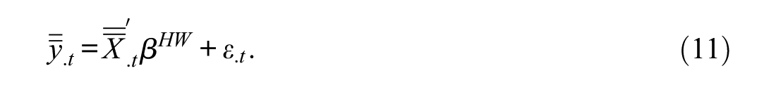
The reader will recognize equation (11) from earlier: it is the model for common trends. We can see from the above equations that $ε_{. t}$ cannot correlate with ${\overset{⌣}{X}}_{it}$ , because the equations are orthogonal. In fact, the model in equation (10) is a two-way fixed effects model, so it is impossible for unmeasured period effects to correlate with ${\overset{⌣}{X}}_{it}$ . To see this, we write the traditional two-way fixed effects estimator as follows (Imai and Kim forthcoming):

{\hat{β}}^{I} = argmi n_{β} \sum_{i = 1}^{N} \sum_{t = 1}^{T} [{(y_{it} - \bar{y}) - ({\bar{y}}_{i .} - \bar{y}) - ({\bar{y}}_{. t} - \bar{y})} - {(X_{it} - \bar{X}) - ({\bar{X}}_{i .} - \bar{X}) - ({\bar{X}}_{. t} - \bar{X})}' β^{I}]^{2} .

(12)

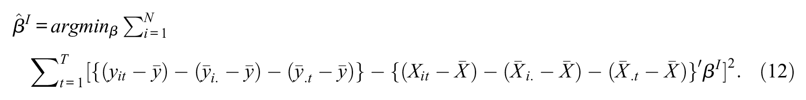
The expression is simplified by centering all variables on cross-sectional units:

{\hat{β}}^{I} = argmi n_{β} \sum_{i = 1}^{N} \sum_{t = 1}^{T} [{({\tilde{y}}_{it} - \bar{\tilde{y}}) - ({\bar{\bar{y}}}_{. t} - \bar{\tilde{y}})} - {({\tilde{X}}_{it} - \bar{\tilde{X}}) - ({\bar{\bar{X}}}_{. t} - \bar{\tilde{X}})}' β^{I}]^{2} .

(13)

We can simplify again by centering on time to eliminate period effects:

{\hat{β}}^{I} = argmi n_{β} \sum_{i = 1}^{N} \sum_{t = 1}^{T} [{({\overset{⌣}{y}}_{it} - \bar{\overset{⌣}{y}})} - {({\overset{⌣}{X}}_{it} - \bar{\overset{⌣}{X}})}' β^{I}]^{2},

(14)

which is the ordinary least squares estimate of equation (10). A technical derivation of the models in equations (10) and (11) using system estimation is provided in the Appendix.

Because ${\tilde{y}}_{it} = {\overset{⌣}{y}}_{it} + {\bar{\bar{y}}}_{. t},$ combining equations (10) and (11) produces a simultaneous equation of the two-way fixed effects model and the model for common trends:

{\tilde{y}}_{it} = \overset{⌣}{X}_{it}^{'} β^{I} + {\bar{\bar{X}}}_{. t}^{'} β^{HW} + u_{it} + ε_{. t} .

(15)

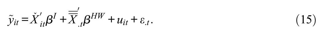
Because the within and between variation are orthogonal, we obtain the general BWI model by stacking equation (15) with the equation for the between model, which gives $y_{it} = β_{0} + {\overset{⌣}{X}}_{it}^{'} β^{I} + {\bar{\bar{X}}}_{. t}^{'} β^{HW} + {\bar{X}}_{i .}^{'} β^{B} + a_{i .} + u_{it} + ε_{. t}$ . Thus, we can regard the equation for the BWI model as a simultaneous equation for three uncorrelated models: the two-way fixed effects model (equation 10), the model for common trends (equation 11), and the between model presented earlier.

There are four primary benefits of the BWI model. First, it provides the homogenous-within effect of common trends, which is not provided in any other model. Second, the model allows for covariance with unmeasured period effects and unmeasured between effects. Third, in contrast to two-way fixed effects models, the model can include time-invariant and unit-invariant variables. Fourth, the model offers these benefits at little cost, as it provides the same idiosyncratic effect as the two-way fixed effects model, and thus it can be used for causal inference in the same way as two-way fixed effects.

Returning to our example of decreasing crime rates in major cities, the BWI model would allow us to evaluate several processes for the decline. $β^{HW}$ would tell us whether a common trend toward antiviolence organization mobilization in major cities contributed to a mean reduction in crime across major cities. $β^{I}$ would tell us whether within-specific-city changes in community organization mobilization contributed to within-specific-city changes in crime rates. $β^{B}$ would tell us whether cities that have, on average, more anticrime community organizations have, on average, lower crime rates. By focusing explicitly on $β^{HW}$ , we would be able to determine whether a common trend toward anticrime organization mobilization had an effect on crime rates in most major cities, producing the national decline in crime during the 1990s.

From a Multilevel Perspective

As mentioned earlier, the BWI model can be regarded as a single equation for three stacked models. We can show this more explicitly by regarding the BWI model as a cross-classified multilevel model. Each it observation is “nested in” cross-sections and time periods. The level 1 equation is $y_{it} = β_{it 0} + {\overset{⌣}{X}}_{it}^{'} β^{I} + u_{it}$ , where $β_{it 0}$ is a random intercept that varies across units and time. We write the level 2 equation to account for both the unmeasured between effect and the unmeasured period effect: $β_{it 0} = β_{0} + {\bar{\bar{X}}}_{. t}^{'} β^{HW} + {\bar{X}}_{i .}^{'} β^{B} + a_{i .} + ε_{. t}$ . Here, we obtain the grand intercept ( $β_{0}$ ), the random variation across units ( $a_{i .}$ ), and the random variation across time $(ε_{. t}$ ). As before, we assume that $a_{i .}$ and $ε_{. t}$ have zero means and normal variances. Plugging the level 2 equation into the level 1 equation yields the BWI model presented above.

An advantage of the multilevel framework is the ability to include random slopes. Including a random slope is equivalent to including a vector of interactions, but random slopes are more efficient (Gelman and Hill 2011:282–83; Heisig, Schaeffer, and Giesecke 2017). This means we can obtain time-varying coefficients without having to rely on interaction coefficients, as in two-way fixed effects models. This reduces the complexity of interpreting time-varying slopes in the BWI model, increases efficiency relative to the interaction-coefficient approach, and helps minimize the risk for type I error. An extended discussion of random slopes is not possible here, but readers can find details on random slope models in Gelman and Hill (2011), Heisig et al. (2017), and Raudenbush and Bryk (2002).

Relation to Bollen and Brand’s Model

It can be shown that the BWI model extends the general panel model introduced by Bollen and Brand (2010). Bollen and Brand’s model is

y_{it} = X_{it}^{'} β_{yt}^{X} + Z_{i .}^{'} β_{yt}^{Z} + λ_{t} a_{i} + e_{it} .

X is a matrix of time-varying variables, which may include within-transformed variables. Z is a matrix of time-invariant variables, which may include cross-sectional unit means. The t subscript indicates that coefficients are allowed to vary across time periods. $λ_{t}$ provides time-varying coefficients for $a_{i}$ . This is a general model in that many panel models are special cases of the general model. For instance, if we specify Z to be a matrix of unit-indicator variables and we assume that there are no time-varying coefficients, we obtain a one-way fixed effects model.

Bollen and Brand’s (2010) model allows for unobserved between effects, but it does not include unobserved period effects or unit-invariant variables. We can expand the model to include unit-invariant variables and unmeasured period effects:

y_{it} = X_{it}^{'} β_{yt}^{X} + Z_{i .}^{'} β_{yt}^{Z} + C_{. t}^{'} β_{yt}^{C} + λ_{t} a_{i} + λ_{i} ε_{. t} + e_{it} .

C is a matrix of unit-invariant variables, which may include common trends. We now include the unmeasured period effect, which was not present in Bollen and Brand’s (2010) model, where $λ_{i}$ is the unit-specific coefficient for the unmeasured period effect. If we specify X to include the idiosyncratic transformation of the time-varying variables, Z to include the between transformation, and C to include the common trends, the model becomes a case of the BWI model with random slopes for all coefficients and a unit-varying unmeasured period effect. If we assume the coefficients and unmeasured between effect do not vary across time, and the unmeasured period effect does not vary across units, then the model is the BWI model introduced earlier. Hence, the BWI model can be viewed as an extension to Bollen and Brand’s (2010) model that allows for unit-invariant variables and unmeasured period effects.

Restrictive Forms

The BWI model implies several restrictive forms that are not currently in use in the applied literature but may be useful to researchers concerned with time heterogeneity.

Case 1: The Cross-Classified Between-Within Model

A first restrictive form exists in cases in which the unmeasured period effect is uncorrelated with X. If the unmeasured period effect does not correlate with X, we can use the within transformation rather than the idiosyncratic transformation. This yields a special case of the between-within model that includes an unmeasured period effect:

y_{it} = β_{0} + {\tilde{X}}_{it}^{'} β^{W} + {\bar{X}}_{i .}^{'} β^{B} + a_{i .} + u_{it} + ε_{. t} .

(16)

This model is identical to the standard between-within model, with the sole exception that now we allow for unobserved time heterogeneity. However, unlike the BWI model, we assume the unmeasured period effect is uncorrelated with the within-transformed variables. When there is no unmeasured period effect ( $ε_{. t}$ = 0), the cross-classified between-within (ccBW) model in equation (16) and the standard between-within model in equation (6) are equivalent.

Case 2: The Random Effects Within Model

A second restrictive form provides an extension to the one-way fixed effects model that allows for unobserved time heterogeneity. Imagine we are not interested in time-invariant variables but are concerned with time heterogeneity. Then we can replace $\bar{X}$ in the ccBW model with a vector of unit-indicator variables, as in a one-way fixed effects model. Because the between variation is eliminated, we can simplify this expression using the within transformation. This gives us the “within equation” for the ccBW model introduced earlier:

{\tilde{y}}_{it} = β_{0} + {\tilde{X}}_{it}^{'} β^{W} + u_{it} + ε_{. t} .

(17)

The only difference between this model and the ccBW model is that we removed the between component. The model in equation (17) is almost identical to the standard one-way fixed effects model (see equation 5), but we now include an unobserved period effect. Hence, the model allows for unobserved time heterogeneity, whereas one-way fixed effects does not. Like ccBW, we assume that $ε_{. t}$ is uncorrelated with $\tilde{X}$ . Because the model in equation (17) is equivalent to the model in equation (5) but allows random variation across time periods, I refer to it as the “random effects within model” (REWM).

Case 3: The Random Effects Within-Idiosyncratic Model

A third restrictive form allows unmeasured period effects to correlate with the within-transformed variables. As before, consider a case in which we are interested only in the over-time variation. Then we can replace $\bar{X}$ in the BWI model with unit-indicator variables. We can regard this model as only using the “within component” of the BWI model. We can express the equation using the within transformation on y and the idiosyncratic transformation on X:

{\tilde{y}}_{it} = \overset{⌣}{X}_{it}^{'} β^{I} + {\bar{\bar{X}}}_{. t}^{'} β^{HW} + u_{it} + ε_{. t} .

(18)

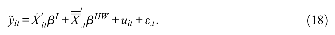
We arrived at this model earlier in equation (15). It is exactly equivalent to the BWI model, minus the between variation. The model allows for covariance with unmeasured period effects, provides the effect of common trends, and can include unit-invariant variables, but it cannot include time-invariant variables. The model therefore offers all the usual benefits of the two-way fixed effects model, while also providing the homogenous-within effect of common trends. I refer to this model as the “random effects within-idiosyncratic model” (REWIM).

Estimation and Covariance Matrix

It is possible to estimate the BWI model and its restrictive forms using generalized least squares (GLS). However, estimates are generally improved with empirical Bayes estimation. Empirical Bayes estimation is more efficient than GLS for nested data structures (Snijders and Bosker 2008:58–59). Furthermore, the estimation framework introduces shrinkage, whereby coefficients are pulled toward the grand mean as a function of sample size and variability, increasing the reliability of otherwise unreliable estimates (Gelman and Hill 2011:477; Gill 2014:138; Raudenbush and Bryk 2002:39–40). The empirical Bayes estimates of random time intercepts also provide a parameter for serial correlation in repeated measurement models (Goldstein, Healy, and Rabash 1994), and so standard errors are intrinsically adjusted for serial correlation, which is not true of least squares estimates.

Using generic notation, the covariance matrix of the estimator is

Ω_{\hat{β}} = (X' V^{- 1} X)^{- 1},

(19)

where X is a matrix of preprocessed data, V is a block-diagonal matrix of variance components, and the empirical Bayes estimator is $\hat{β} = (X' V^{- 1} X)^{- 1} X' V^{- 1} y$ . The BWI covariance matrix is block-diagonal, where the diagonal blocks are the covariance matrices for each estimator and the off-diagonal entries are 0 matrices:

Ω_{\hat{β}}^{BWI} = [\begin{matrix} Ω_{{\hat{β}}^{B}} & 0 & 0 \\ 0 & Ω_{{\hat{β}}^{HW}} & 0 \\ 0 & 0 & Ω_{{\hat{β}}^{I}} \end{matrix}] .

In practice, empirical Bayes estimation can be implemented using standard strategies of restricted maximum likelihood estimation and Gibbs sampling (Gelman and Hill 2011:392–98; Raudenbush and Bryk 2002:44–48). Thus, the models can be implemented using existing multilevel modeling software packages such as Stata, SAS, and R. The open-source R software package rewie provides functionality to implement the models (Duxbury 2020).

Model Selection

A two-stage Hausman testing procedure can be used to aid in model selection (Arellano 1993; Hausman 1978; Wooldridge 2010). The Hausman test evaluates the equivalence of an efficient but possibly inconsistent estimator to an inefficient but consistent estimator. It is commonly used to evaluate whether a one-way fixed effects model is preferred to a random effects model, in which a significant result favors one-way fixed effects. Because one-way fixed effects is more efficient than two-way fixed effects but is inconsistent when there is an unmeasured period effect, we can use the test to adjudicate between the two models. First, we test whether one-way fixed effects is preferred to random effects. If the result is significant, we should favor models that rely on the within transformation (one-way fixed effects, REWM, ccBW). Second, we test two-way fixed effects against one-way fixed effects. If the result is significant, we should prefer models that rely on the idiosyncratic transformation (two-way fixed effects, REWIM, BWI).

Hausman tests are widely used for panel model selection, but they tend to produce significant results in large sample spaces even when gains in consistency are minor. One option in these instances is to evaluate improvements in model fit. Bollen and Brand (2010:12–14) recommended several model fit criteria that can aid in model selection, the most familiar of which from a multilevel modeling perspective are the root mean squared error of approximation and Bayesian information criteria. In general, the best fitting model should be preferred. However, note that models that use different transformations of the response variable cannot be compared. For instance, if we first within transform our variables before estimating a REWM, we cannot compare the fit criteria with BWI, because BWI pools all variation in the response, whereas REWM only examines within variation.

In cases in which two competing models use different dependent variable transformations, we can use between-model comparisons of coefficients to inform model selection. When an unmeasured period effect correlates with the within-transformed variables, REWM coefficients will typically be noticeably smaller than one-way fixed effects coefficients because of shrinkage to the grand mean. If one-way fixed effects and REWM provide noticeably different estimates for the same coefficients, this is evidence that the unmeasured period effect correlates with the within-transformed variables. Hence, models that allow for correlation with unmeasured period effects should be preferred.

Intraclass correlations coefficients (ICC) can be used for exploratory analysis. The ICC gives the proportion of variance at each level (Raudenbush and Bryk 2002). If the within variation is far greater than between variation, which is often true of large-T data, then REWM and REWIM are likely appropriate. If the between variation is sizable, as in large-N data, BWI and ccBW are appealing choices. If the idiosyncratic variation is sizable, either REWIM or BWI are likely necessary.

Summary

I introduced a model that provides the effect of common trends and allows for covariance with unmeasured period effects. The BWI model can include unit-invariant and time-invariant variables and time-varying coefficients, and it allows for covariance with unmeasured between effects without sacrificing any of the utility of two-way fixed effects for causal inference. Restrictive forms offer alternatives to one-way fixed effects (REWM), two-way fixed effects (REWIM), and between-within models (ccBW) by allowing for unobserved time heterogeneity. I will now illustrate use of the BWI model and its restrictive forms in an empirical analysis of state incarceration rates.

Empirical Example: Time-Varying Politics of Mass Incarceration

In 1972, the national incarceration rate began an upward march that would not ebb until 2008. Accounts seeking to explain this rise emphasize the national character of mass incarceration (Garland 2001; Gottschalk 2006; Simon 2007; Western 2006) and differences in state trajectories (Campbell and Schoenfeld 2013; Lynch 2009; Page 2011; Schoenfeld 2018). Although the United States at large experienced a uniform increase in incarceration, roughly 90 percent of the growth in the prison population was within state prisons and, as shown in Figure 1, there was sizable state heterogeneity in incarceration trajectories (Campbell 2018). Prior analyses focus on change within states using either one-way fixed effects models (Enns 2016; Greenberg and West 2001; Western 2006) or two-way fixed effects models (Keen and Jacobs 2009; Muller 2012). However, because neither model can simultaneously account for unmeasured period effects and the effect of common trends, it is unclear whether results from studies using one-way fixed effects analyses are biased, or whether results from studies using two-way fixed effects are misleading because they eliminate common trends.

Figure 1.

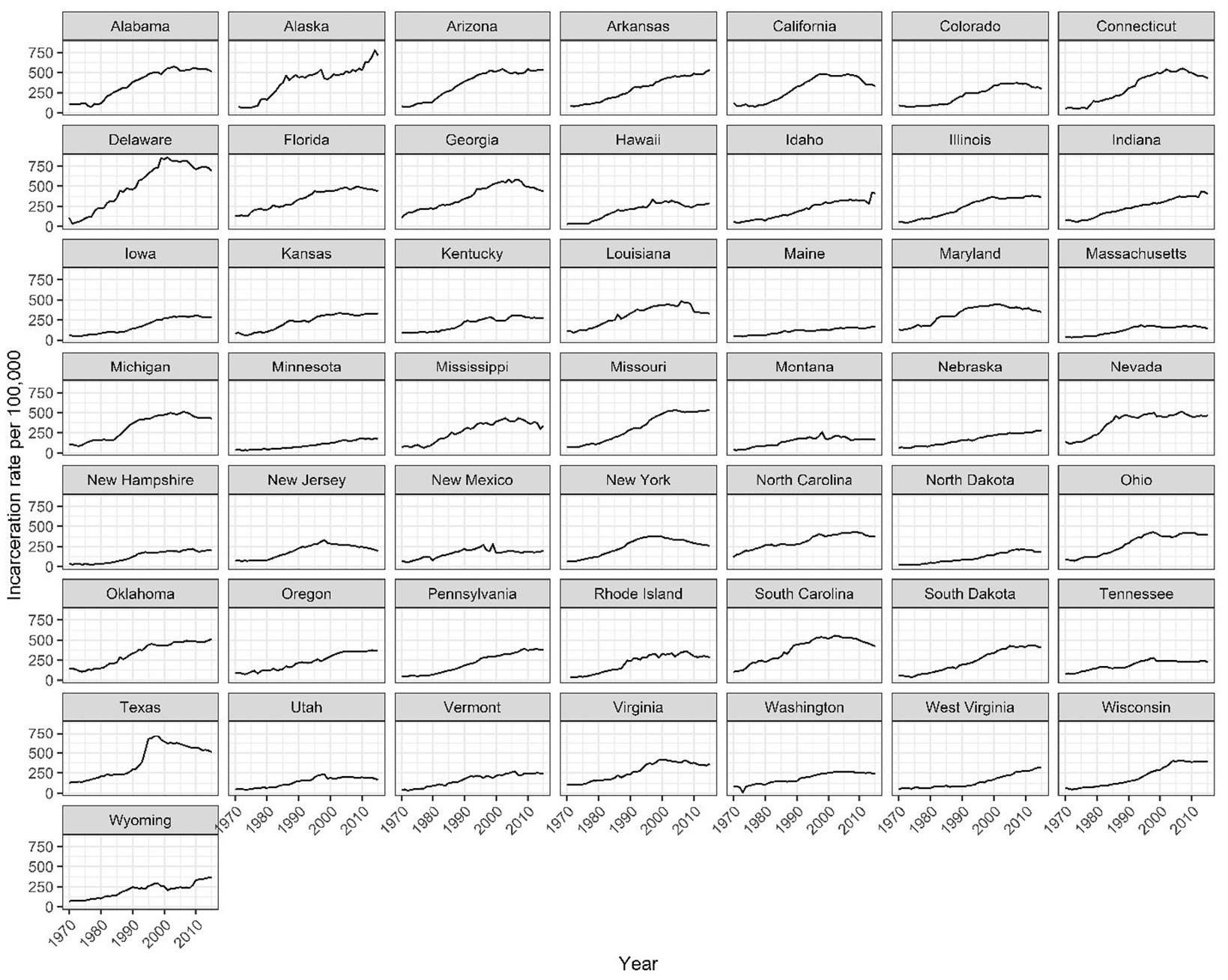
Incarceration rate in 50 states, 1970 to 2015.

To illustrate this point, Table 3 presents linear models predicting state incarceration rates between 1970 and 2015 including only state fixed effects, only time fixed effects, and both state and time fixed effects. The R² value in model 1 is .36, meaning that, despite large-T data, 36 percent of the variation is between variation. Model 2 includes only time fixed effects, showing that 51 percent of the variation influenced all states equally; that is, half the variation in state incarceration rates, and 79 percent of the within variation, can be attributed to common trending. Model 3 includes both time and state fixed effects. The R² value is an impressive .87, indicating that without accounting for any theoretically informative variables, we eliminated almost 90 percent of the variation in state incarceration rates. Studies using two-way fixed effects can therefore only estimate the idiosyncratic effects that explain a minority of the variation in incarceration.⁴

Table 3.

Intercept-Only Models of Incarceration Rates in 50 States, 1970 to 2015 (NT = 2,300)

	Model 1: State FE	Model 2: Year FE	Model 3: State and Year FE
R ²	.355	.513	.868
1 –R²	.645	.487	.132
Within R²	0	.793	.793
F	25.33***	52.62***	153.40***
Intercept	363.135*** (18.355)	79.374*** (15.780)	196.010*** (11.765)

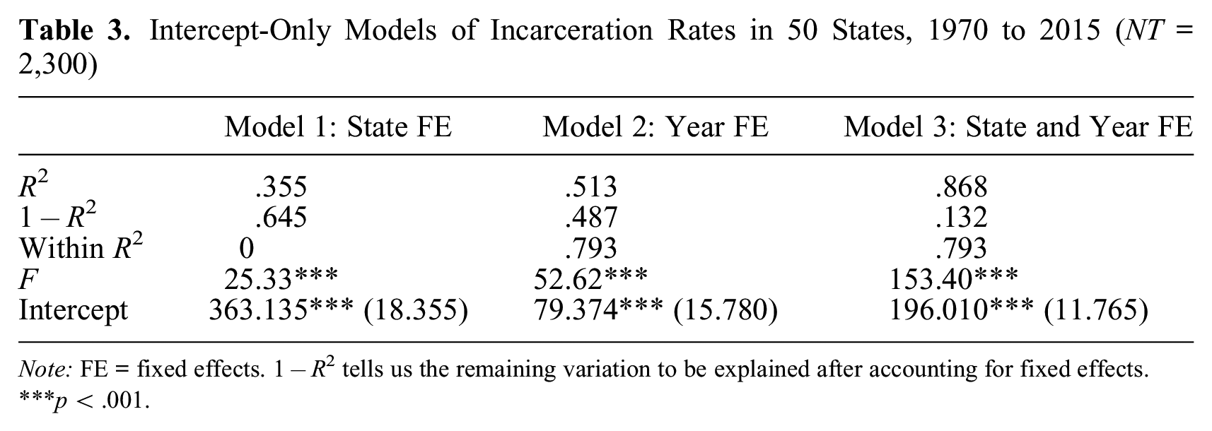
Note: FE = fixed effects. 1 –R² tells us the remaining variation to be explained after accounting for fixed effects.

***

p < .001.

I now examine determinants of state incarceration rates, with a focus on how attention to the level of variation affects conclusions about the politics of mass incarceration. Political accounts argue that Republican politics drove up the incarceration rate (Alexander 2010; Beckett 1997; Weaver 2007). Yet it is unclear at what level Republican politics mattered most, whether the influence of Republican politics was top down or bottom up, and whether the effects of Republican politics were consistent across the entirety of mass incarceration.

Regarding level of variation, accounts emphasizing state heterogeneity suggest that conservative alliances with penal actors in certain states contributed to state heterogeneity in the pacing and timing of mass incarceration (Campbell 2018; Campbell and Schoenfeld 2013; Lynch 2009; Page 2011; Schoenfeld 2018). Other scholars emphasize how tough-on-crime politics vaulted the Republican Party to national dominance, leading to a flurry of tough-on-crime national legislation (Beckett 1997; Simon 2007; Weaver 2007). Regarding direction of political influence, some accounts of national politics argue that public influence was largely ignorable (Beckett 1997; Simon 2007), whereas others suggest that penal actors were driven to tough-on-crime politics by highly punitive conservative constituencies that were most influential at local levels (Enns 2016). Regarding temporal variation, some scholars characterize mass incarceration as a Republican effort (Beckett 1997; Weaver 2007), yet others highlight the “purpling” of punishment in the 1990s (Gottschalk 2006; Page 2011; Simon 2007), when both Republican and Democratic political leaders began to advance tough-on-crime agendas.

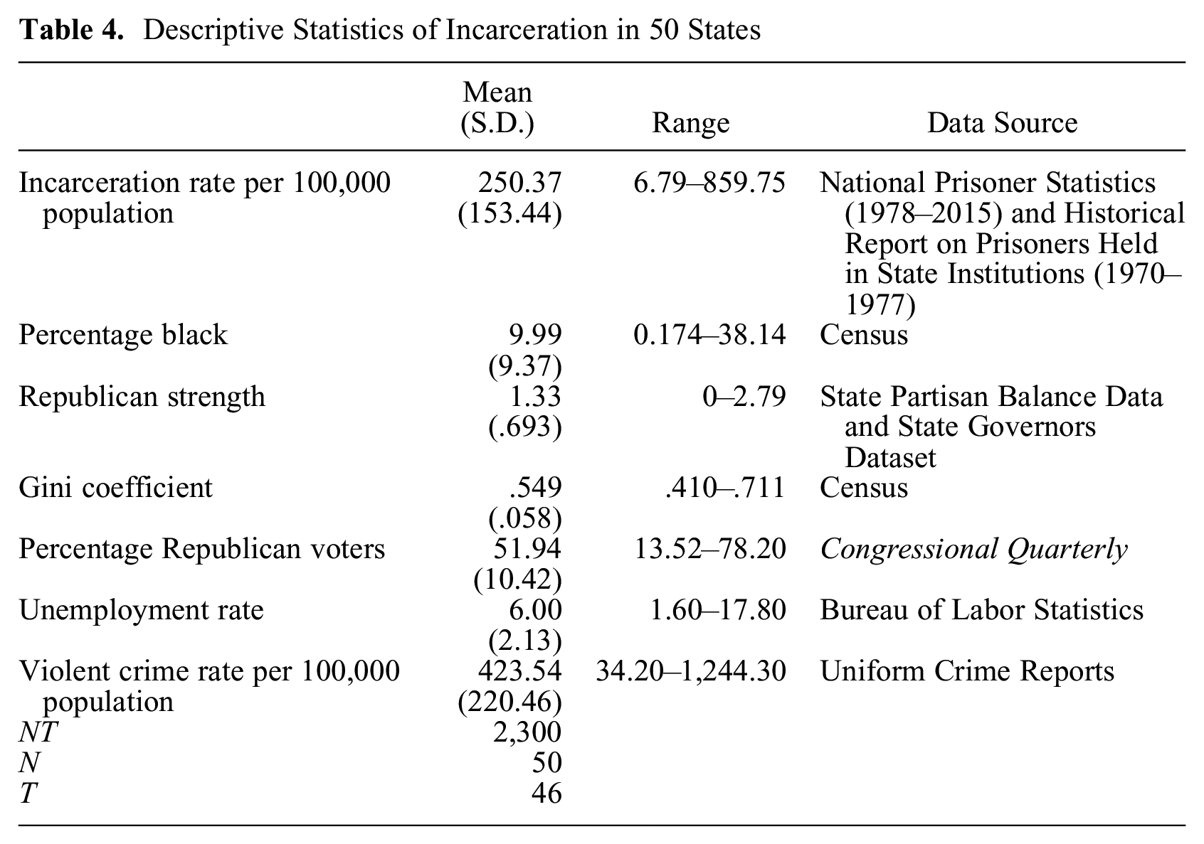
The BWI model and its restrictive forms offer the ability to examine each possibility. The homogenous-within effect of Republican influence offers insight to common trends among states, and the idiosyncratic effect gives insight to state-specific over-time trajectories. Random slopes also provide a strategy to assess whether the effect of Republican influence varied over time. I examine these possibilities by constructing a data set of state incarceration rates. The dependent variable is the incarceration rate per 100,000 population. I measure Republican Party strength as the proportion of Republican seats in the state house plus the proportion of Republican seats in the state senate plus a value of 1 if the governor is Republican. I measure bottom-up Republican support as the percentage of Republican Party voters in the most recent national election. The violent crime rate, unemployment rate, black population size, and Gini coefficient are also included. Table 4 describes each variable and data source.

Table 4.

Descriptive Statistics of Incarceration in 50 States

	Mean(S.D.)	Range	Data Source
Incarceration rate per 100,000 population	250.37(153.44)	6.79–859.75	National Prisoner Statistics (1978–2015) and Historical Report on Prisoners Held in State Institutions (1970–1977)
Percentage black	9.99(9.37)	0.174–38.14	Census
Republican strength	1.33(.693)	0–2.79	State Partisan Balance Data and State Governors Dataset
Gini coefficient	.549(.058)	.410–.711	Census
Percentage Republican voters	51.94(10.42)	13.52–78.20	Congressional Quarterly
Unemployment rate	6.00(2.13)	1.60–17.80	Bureau of Labor Statistics
Violent crime rate per 100,000 population	423.54(220.46)	34.20–1,244.30	Uniform Crime Reports
NT	2,300
N	50
T	46

The next step is to determine which model best represents the data. To do so, I first assess how much variation exists at each level of the response. The ICC results are equivalent to results in Table 3, but I present them here to build intuition. The ICC for states is .352, meaning that 35 percent of the variance is among states. The ICC for time is .512, and the idiosyncratic ICC is .136. Of the within variation, 79 percent is unit-invariant trending (ICC = .790), and only 21 percent is idiosyncratic (ICC = .210). Random effects, ccBW, and BWI are therefore appealing choices, as the between-variation is sizable. An auxiliary Hausman test (Wooldridge 2010) of random effects against one-way fixed effects is significant (χ² = 285.63, p < .001), meaning random effects coefficients are inconsistent. The test also returns a significant result when comparing REWM with two-way fixed effects (χ² = 59.52, p < .001), meaning that models that use the idiosyncratic transformation should be preferred. Thus, the BWI model is the clear choice.

Table 5 presents results from panel models. Models 1 and 2 present one-way and two-way fixed effects models. The one-way model shows positive effects for percent black, Republican Party strength, the Gini coefficient, unemployment rate, and violent crime rate but an insignificant effect for percentage Republican voters. Model 2 presents the two-way fixed effects results. Here, the percentage black population, Gini coefficient, and violent crime rate are again significant, but Republican Party strength and the unemployment rate are insignificant. Furthermore, the percentage Republican voters is now positive and significant, and the coefficients for percentage black, the Gini coefficient, and violent crime rate are substantially attenuated.

Table 5.

Panel Models of Incarceration Rates in 50 States

	Model 1: One-Way FE	Model 2: Two-Way FE	Model 3: REWM	Model 4: REWIM	Model 5: ccBW	Model 6: BWI
β^W
Percentage black	20.53***		8.71***		8.53***
	(1.76)		(1.57)		(1.59)
Republican strength	24.44***		5.79*		5.67*
	(2.74)		(2.45)		(2.47)
Gini coefficient	1,436.71***		436.99***		444.34***
	(39.67)		(63.97)		(64.29)
Percentage Republican voters	.176		1.64***		1.68***
	(.193)		(.268)		(.272)
Unemployment rate	−4.91***		−1.22		−1.22
	(.842)		(1.17)		(1.17)
Violent crime rate per 100,000 population	.086***		.062***		.059***
	(.014)		(.014)		(.014)
β^I
Percentage black		7.68***		7.88***		7.69***
		(1.60)		(1.57)		(1.60)
Republican strength		4.41		4.56		4.42
		(2.48)		(2.46)		(2.48)
Gini coefficient		346.58***		340.14***		346.59***
		(66.33)		(65.97)		(66.32)
Percentage Republican voters		1.74***		1.70***		1.74***
		(.275)		(.271)		(.278)
Unemployment rate		−.862		−.872		−.873
		(1.19)		(1.19)		(1.19)
Violent crime rate per 100,000 population		.057***		.060***		.057***
		(.014)		(.014)		(.014)
β^HW
Percentage black				85.13***		85.07***
				(19.14)		(19.14)
Republican strength				61.14*		61.15*
				(26.00)		(25.99)
Gini coefficient				388.20		388.19
				(317.84)		(317.72)
Percentage Republican voters				.579		.573
				(.611)		(.611)
Unemployment rate				−7.43*		−7.43*
				(2.91)		(.291)
Violent crime rate per 100,000 population				.360***		.361***
				(.087)		(.087)
β^B
Percentage black					2.67	2.67
					(1.59)	(1.59)
Republican strength					−3.42	−3.41
					(40.32)	(40.33)
Gini coefficient					1,143.74*	1,148.58*
					(573.50)	(573.51)
Percentage Republican voters					4.61	4.60
					(2.46)	(2.46)
Unemployment rate					1.38	1.36
					(13.59)	(13.59)
Violent crime rate per 100,000 population					.250***	.250***
					(.077)	(.078)
Intercept			14.81	2.43	−733.67*	−748.24*
			(11.84)	(3.34)	(364.67)	(364.57)
Variance components (S.D.)
Idiosyncratic (level 1)			51.24	51.20	51.23	51.19
Time (level 2)			74.36	18.79	74.27	18.78
States (level 2)					51.23	73.45
R² (total)	.67	.89	.31	.52	.43	.65
$R_{φ}^{2}$ (within)	.70	.80	.47	.81	.48	.81
$R_{u}^{2}$ (idiosyncratic)		.07	.19	19	.19	.19
$R_{ε}^{2}$ (time)			.55	.97	.55	.97
$R_{a}^{2}$ (between)					.36	.36
AIC			18,770	18,636	18,925	18,791
BIC			18,819	18,718	19,012	18,912

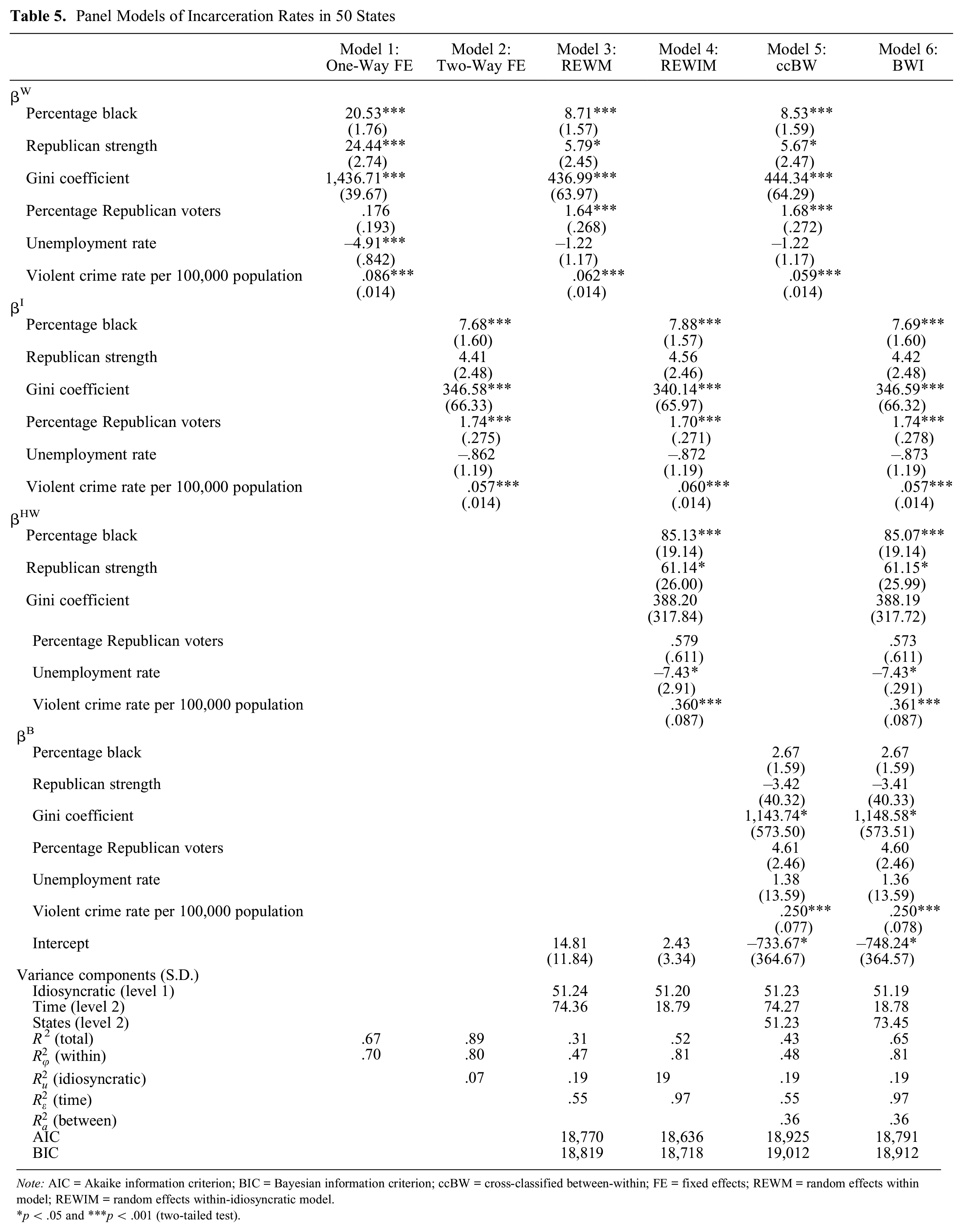
Note: AIC = Akaike information criterion; BIC = Bayesian information criterion; ccBW = cross-classified between-within; FE = fixed effects; REWM = random effects within model; REWIM = random effects within-idiosyncratic model.

p < .05 and ***p < .001 (two-tailed test).

How do we account for these differences? Are the effect sizes and significance in model 1 an artifact of time heterogeneity? Or are the attenuated coefficients in model 2 a result of purging common trends? Model 3 presents results from REWM. The coefficients in REWM are far smaller than the one-way fixed effects coefficients. In fact, the REWM coefficients are more similar in size to the two-way fixed effects coefficients. Percentage black, Republican strength, the Gini coefficient, and violent crime rate coefficients are positive and significant. However, the percentage of Republican voters is now positive and significant, and the unemployment rate is insignificant. Consistent with Hausman test results, shrinkage in the REWM coefficients provides additional evidence that there is covariance with an unmeasured period effect.

Model 4 allows for covariance with unmeasured period effects using REWIM. Specifying separate models for the idiosyncratic variables and common trends yields a substantial gain in model fit, whereby both the Akaike information criterion (AIC) and Bayesian information criterion (BIC) decline between models 3 and 4, and the within R² value increases from .47 to .81. As expected, estimates of β^I are (approximately) equal in models 2 and 4. However, we now also obtain estimates of β^HW. The percentage black population has a positive homogenous-within effect. A 1 percent mean increase in the percentage black population increases the mean state incarceration rate by 85 people per 100,000 population. We further see both an idiosyncratic and a homogenous-within effect of violent crime on the incarceration rate. The homogenous-within effect for the unemployment rate is negative and significant, indicating the significance of the unemployment rate in model 1 can be attributed to national, rather than idiosyncratic, declines in unemployment, which has been documented elsewhere (Garland 2001; Western 2006).

We also see a positive homogenous-within effect for Republican Party strength. This result indicates that the within effect of Republican Party strength can be attributed entirely to the dominance of conservative politics in the national political arena, as Republican Party strength has no significant idiosyncratic effect on state-specific change. Turning to bottom-up politics, the homogenous-within effect for percent Republican voters is insignificant, but the idiosyncratic effect is positive and significant. Thus, national trends in incarceration were driven by Republican leadership, but state trajectories were moved by conservative voters.

Models 5 and 6 present results from ccBW and BWI. Consistent with theoretical results, the ccBW within coefficients are close approximates of the REWM coefficients, and the idiosyncratic and homogenous-within coefficients of BWI are identical to REWIM. The between coefficients in both ccBW and BWI are equivalent. Interpreting the between coefficients, we see that states with more income inequality (higher Gini coefficients), on average, have higher incarceration rates. States with higher mean violent crime rates also tend to have higher incarceration rates. Both Republican politics variables have insignificant between effects. This means that although Republican politics played an important role in the time-varying politics of mass incarceration, partisanship mattered little for differences in state averages.

Comparing between models, we see that BWI is the most informative, with lower AIC and BIC compared with ccBW. Although we cannot compare AIC and BIC between REWIM and BWI, because the response variables are a different transformation, we can compare the total variation explained. The inclusion of between effects in BWI increases the total R² value from .52 in REWIM to .65 in BWI. Furthermore, decomposing the within effect increases the within R² value from .7 in model 1 to .81 in models 4 and 6. Including a time intercept also dramatically improves the idiosyncratic variation explained, increasing the idiosyncratic R² value from .07 in two-way fixed effects to .19 in models 3 to 6.

The next step is to allow for time-varying Republican Party strength coefficients using random slopes. Because the interest is in temporal variation rather than between variation, I present results only from REWIM in Table 6. The variance component for the Republican strength slope is .51, indicating that there is variance across time in the effect of Republican leadership. The AIC and BIC decline compared with model 4, meaning that information is gained by including random slopes. After accounting for time-varying coefficients, the Republican Party strength idiosyncratic coefficient is positive and significant. This means that there is temporal variation in the idiosyncratic effect of Republican leadership, which aligns with prior accounts of the “purpling” of punishment in the 1990s (Page 2011; Simon 2007).

Table 6.

Random Slopes REWIM of Incarceration Rates in 50 States

	Model 7: Random Slopes REWIM
β^I
Percentage black	7.90*** (1.57)
Republican strength	4.52* (2.26)
Gini coefficient	340.44*** (65.98)
Percentage Republican voters	1.69*** (.271)
Unemployment rate	−.878 (1.19)
Violent crime rate per 100,000 population	.060*** (.014)
β^HW
Percentage black	84.71*** (19.13)
Republican strength	60.99* (25.99)
Gini coefficient	399.01 (317.68)
Percentage Republican voters	.550 (.611)
Unemployment rate	−7.43* (2.91)
Violent crime rate per 100,000 population	.359*** (.087)
Intercept	2.39 (3.34)
Variance components (S.D.)
Idiosyncratic (level 1)	51.20
Time (level 2)	18.79
Republican strength time slope	.51
R² (total)	.53
$R_{φ}^{2}$ (within)	.81
$R_{u}^{2}$ (idiosyncratic)	.19
$R_{ε}^{2}$ (time)	.98
AIC	18,640
BIC	18,733

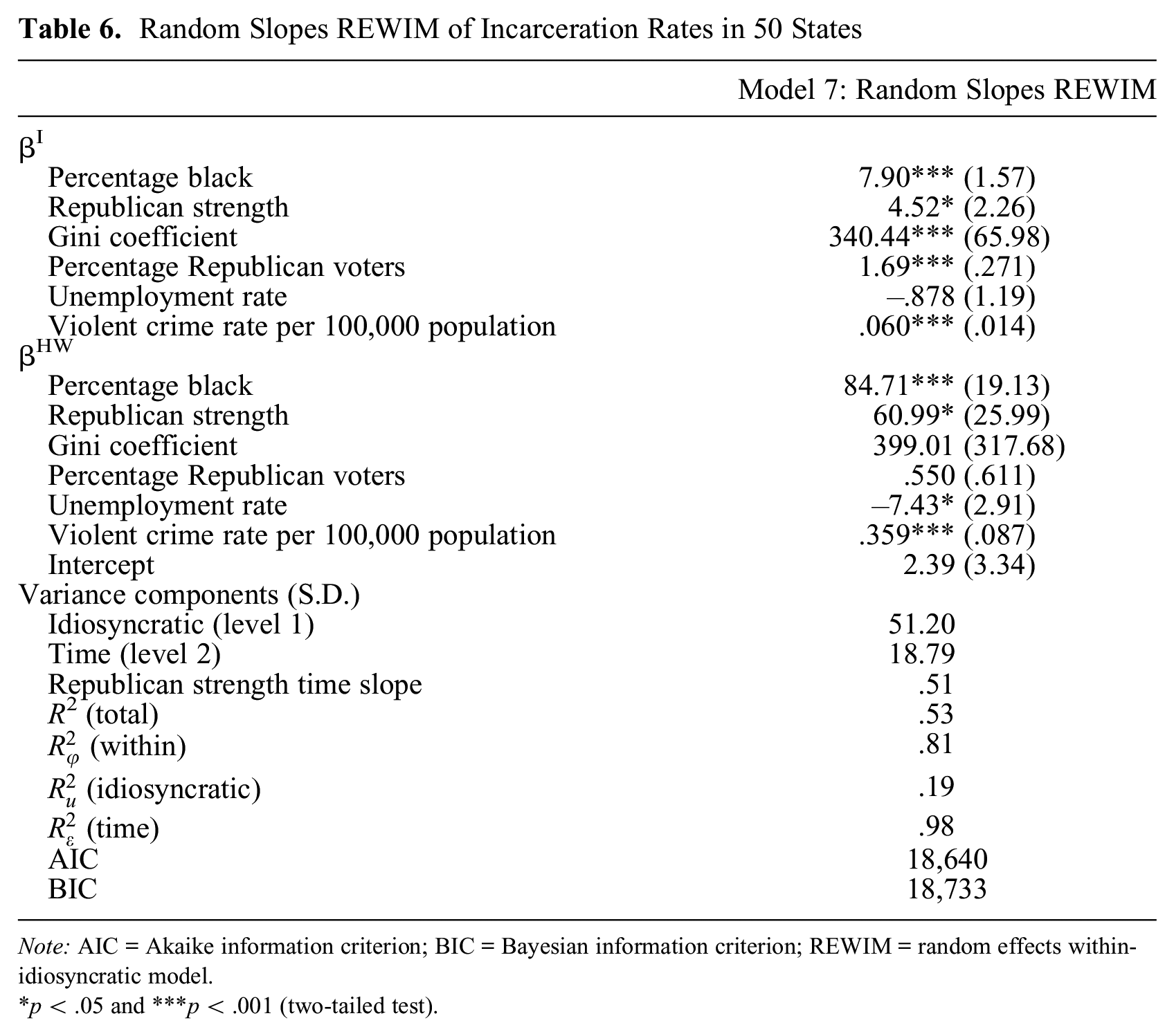
Note: AIC = Akaike information criterion; BIC = Bayesian information criterion; REWIM = random effects within-idiosyncratic model.

p < .05 and ***p < .001 (two-tailed test).

Collectively, these results illustrate how attention to the level of variation can shape substantive conclusions. The only coefficient that yields the same conclusion regardless of modeling strategy is the crime rate. By paying attention to the level of variation, we get a more nuanced story about the politics of mass incarceration. Past research emphasizes the role of conservative politics, but results reveal that top-down conservative politics had its largest effect on common trends, and the local effect of Republican leadership varied across time. By contrast, bottom-up support for Republican politics mattered little for common trends but had a sizable effect on state-specific change. We learn that Republican leadership shaped the national character of mass incarceration, yet Republican voters contributed to the “varieties of mass incarceration” experienced across states (Campbell 2018).

Conclusion

This study introduced a general panel model for unobserved time heterogeneity that also allows for covariance with unmeasured between effects, can include time-invariant and unit-invariant variables, and provides the coefficient for common trends. The two-way fixed effects model can control for unmeasured period effects and unmeasured between effects, but it cannot include unit-invariant and time-invariant variables or be used to examine common trends. Common trends may be substantively informative in many research settings. As we saw in the case of mass incarceration, even though 90 percent of the growth in incarceration was in state prisons, 51 percent of the variance in the incarceration rate was common trending. A two-way fixed effects model would lead us to conclude that Republican voters drove state incarceration rates, yet accounting for common trends tells us that, in fact, the common trend in incarceration rates is explained by Republican leadership, not Republican constituencies.

Future work would benefit from examining common trends in panel data analysis. A great appeal of the BWI framework is that common trends can be examined while still estimating the idiosyncratic effect typically provided by two-way fixed effects models. Common trends may be especially informative in studies in which cohort effects are suspected. Student grade point averages may correlate with a trend toward “helicopter parenting,” where parents increasingly enforce longer study hours and barter with teachers for better grades (Calarco 2020). National crime declines may be associated with an increase in antiviolence organizations in major cities (Sharkey et al. 2017). Increases in tenure standards may correlate with increased publishing frequency among scientists (Weisshaar 2017). All of these possibilities can be explored by examining common trends.

Along with the benefits elaborated here, the BWI model offers several other utilities. First, in addition to time interactions, idiosyncratic coefficients are biased if there is an unmeasured interaction with a cross-sectional unit. The models introduced here can address this possibility in a straightforward fashion by including random slopes that vary across cross-sections rather than across time. Cross-sectional random slopes can also be included in REWIM and REWM, although there will be no random cross-section intercept because the cross-section means are zero.

Second, the BWI model allows more efficient analysis of heterogeneous treatment in studies concerned with causal inference. Analysts typically stratify two-way fixed effects models by group to account for heterogeneous treatment effects, but this strategy is inefficient because each interaction decreases degrees of freedom and is prone to false discovery (Green and Kern 2012; Tian et al. 2014). Because the BWI model provides the idiosyncratic effect in a multilevel set up, it is straightforward to specify a random slope on a treatment effect to allow it to vary randomly across a group of interest. This allows for heterogeneous treatment but is more efficient than the interaction-coefficient approach.

To be sure, there are situations in which the BWI model and its restrictive cases are not appropriate. The models rely on within-unit change, so in scenarios in which the within-transformed or idiosyncratic-transformed data are not strictly exogenous, neither the BWI model nor its restrictive forms should be applied. For instance, the models are not appropriate if the transformed data are nonstationary (see Wooldridge 2010). Nor should the models be used if there is evidence of simultaneous causality, for which instrumental variables or dynamic panel models may be necessary (e.g., Arellano and Bond 1991).

Future research might extend this framework to discrete outcomes. Although it is straightforward to preprocess the data and estimate one of the models described in Table 2 with a discrete outcome, the behaviors of such models are not well understood. Estimates from between-within models can be biased when used to model discrete outcomes (Allison 2009). Hence, there may be comparable biases in BWI models.

In summary, other panel models allow for unobserved unit heterogeneity, but few alternative models exist for unobserved time heterogeneity. The two-way fixed effects model is the most widely used model for unobserved time heterogeneity, but the model is inefficient, limited in the types of variables that can be included, and cannot be used to explore common trends. The BWI model offers all the benefits of two-way fixed effects models, but it can also include time-invariant and unit-invariant variables, and it provides the effect of common trends. The BWI model is thus a useful and relatively familiar model for panel data analysis in the presence of unobserved time heterogeneity, and it provides greater utility for the analysis of common trends than do other available models.

Footnotes

Appendix

This Appendix applies Baltagi’s (2006) derivation of the Mundlak (1978) model to show that the model in equation (15) is a reexpression of the one-way fixed effects model in equation (5). Consider the following one-way fixed effects equation:

(A1)

{\tilde{y}}_{it} = \tilde{X}'_{it} β^{W} + ψ_{it} .

The time effects are a linear function of the averages of all explanatory variables across observations:

(A2)

ε_{. t} = \bar{\bar{X_{. t}^{'}}} π + ϵ_{. t},

where $ϵ_{. t}$ and $u_{it}$ are independent and identically distributed, normal variables with mean zero and normal variance, $ϵ_{. t} ~ N (0, σ_{ϵ}^{2})$ , $u_{it} ~ N (0, σ_{u}^{2})$ , and $\bar{\bar{X_{. t}^{'}}}$ is a vector of time means of the within variation for the explanatory variables.

We write the one-way fixed effects model in vector form:

(A3)

\tilde{y} = \tilde{X} β^{W} + P \tilde{X} π + τ,

where P is a matrix that averages the observations for each time period, and $τ = A_{ε} ϵ + u$ , $A_{μ} = I_{N}$ ⊗ $l_{T}$ , where $I_{N}$ is an identity matrix with N dimensions and $l_{T}$ is a vector of ones of dimension T. P is the projection matrix, $P = A_{ε} (A_{ε}' A_{ε})^{- 1} A_{ε}'$ .

Because $P^{2} = P$ and $P A_{ε} = A_{ε}$ , premultiplying equation (A4) by P yields

(A4)

P \tilde{y} = P \tilde{X} (β^{W} + π) + P τ .

GLS on equation (A4) yields $(\hat{β^{W} + π}) = (\tilde{X}' P \tilde{X})^{- 1} \tilde{X}' P \tilde{y}$ , which is the GLS estimator of $β^{HW}$ in equation (11). We obtain $β^{I}$ by premultiplying by Q, where $Q = I_{NT} - P$ is a matrix that obtains deviations from the time-means of the within variation:

(A5)

Q \tilde{y} = Q \tilde{X} β^{W} + Q τ

because QP = 0. GLS on equation (A6) obtains $\hat{β^{I}} = ({\tilde{X}}^{'} Q \tilde{X})^{- 1} \tilde{X}' Q \tilde{y}$ , which is the usual two-way fixed effects estimator.

Stacking the system of equations yields

(A6)

(\begin{matrix} P \tilde{y} \\ Q \tilde{y} \end{matrix}) = (\begin{matrix} P \tilde{X} \\ Q \tilde{X} \end{matrix}) β^{W} + (\begin{matrix} P \tilde{X} \\ 0 \end{matrix}) π + (\begin{matrix} P τ \\ Qu \end{matrix}),

with a mean zero for the system error vector and covariance matrix:

(A7)

Ω = (\begin{matrix} σ_{φ}^{2} P & 0 \\ 0 & σ_{u}^{2} Q \end{matrix}),

where $σ_{φ}^{2} = σ_{u}^{2} + σ_{ϵ}^{2}$ . Because $I_{NT} = P + Q$ , GLS on equation (A7) yields

(A8)

\tilde{X}' \tilde{y} = {\tilde{X}}^{'} \tilde{X} β^{W} + \tilde{X}' P \tilde{y} π,

and

(A9)

{\tilde{X}}^{'} P \tilde{y} = {\tilde{X}}^{'} P \tilde{X} β^{W} + {\tilde{X}}^{'} P \tilde{X} π .

Subtracting equation (A9) from equation (A8), we obtain $\tilde{X}' Q \tilde{y} = ({\tilde{X}}^{'} Q \tilde{X}) β^{W} \to^{yields}$ $\hat{β^{I}} = ({\tilde{X}}^{'} Q \tilde{X})^{- 1} \tilde{X}' Q \tilde{y}$ . Solving equation (A9) yields $\hat{β^{HW}} = (\hat{β^{W} + π}) = (\tilde{X}' P \tilde{X})^{- 1} \tilde{X}' P \tilde{y}$ .

Similarly, GLS on equation (A6) yields

(A10)

(\frac{\tilde{X}' P \tilde{y}}{σ_{φ}^{2}} + \frac{\tilde{X}' Q \tilde{y}}{σ_{u}^{2}}) = (\frac{\tilde{X}' P \tilde{X}}{σ_{φ}^{2}} + \frac{\tilde{X}' Q \tilde{X}}{σ_{u}^{2}}) β^{W} + (\frac{\tilde{X}' P \tilde{X}}{σ_{φ}^{2}}) π,

and

(A11)

\frac{\tilde{X}' P \tilde{y}}{σ_{φ}^{2}} = (\frac{\tilde{X}' P \tilde{X}}{σ_{φ}^{2}}) (β^{W} + π) .

Equation (A11) yields $\hat{β^{HW}} = (\tilde{X}' P \tilde{X})^{- 1} \tilde{X}' P \tilde{y}$ . Furthermore, by subtracting equation (A11) from equation (A10), we obtain $\tilde{X}' Q \tilde{y} = ({\tilde{X}}^{'} Q \tilde{X}) β^{W}$ and $\hat{β^{I}} = ({\tilde{X}}^{'} Q \tilde{X})^{- 1} \tilde{X}' Q \tilde{y}$ . This system derivation proves that the model in equation (15) is a reexpression of the one-way fixed effects model.

Acknowledgements

I thank Ken Bollen for helpful comments on an earlier draft of this article. I also thank Hui Zheng, John Casterline, and Lora Phillips for helpful conversations that sparked this study.

ORCID iD

Scott W. Duxbury

Notes

Author Biography

Scott W. Duxbury is an assistant professor of sociology at the University of North Carolina at Chapel Hill. His substantive research investigates racial disparities in the criminal justice system, public opinion, and the network dynamics of criminal markets. His methodological research develops statistical methods for panel data and network analysis. His work has appeared in outlets such as American Sociological Review, the American Journal of Sociology, and Social Forces.

References

Alexander

Michelle

. 2010. The New Jim Crow: Mass Incarceration in the Age of Colorblindness. New York: New Press.

Allison

Paul

. 2009. Fixed Effects Regression. Thousand Oaks, CA: Sage.

Angrist

Joshua

Pischke

Jorn-Steffen

. 2009. Mostly Harmless Econometrics: An Empiricist’s Companion. Princeton, NJ: Princeton University Press.

Arellano

Manuel

. 1993. “On the Testing of Correlated Effects with Panel Data.” Journal of Econometrics 59(1):87–97.

Arellano

Manuel

Bond

Stephen

. 1991. “Some Test of Specification for Panel Data: Monte Carlo Evidence and an Application to Employment Equations.” Review of Economic Studies 58(2):277–97.

Baltagi

Badi H.

2006. “An Alternative Derivation of Mundlak’s Fixed Effects Results Using System Estimation.” Econometric Theory 22(6):1191–94.

Baltagi

Badi H.

2013. Econometric Analysis of Panel Data. West Sussex, UK: John Wiley.

Beckett

Katherine

. 1997. Making Crime Pay: Law and Order in Contemporary American Politics. Oxford, UK: Oxford University Press.

Bertrand

Marianne

Duflo

Esther

Mullainathan

Sendhil

. 2004. “How Much Should We Trust Differences-in-Differences Estimators?” Quarterly Journal of Economics 119(1):249–75.

10.

Bollen

Kenneth A.

Brand

Jennie E.

2010. “A General Panel Model with Random and Fixed Effects: A Structural Equation Approach.” Social Forces 89(1):1–34.

11.

Bruderl

Josef

Ludwig

Volker

. 2015. “Fixed-Effects Panel Regression.” Pp. 327–57 in Sage Handbook of Regression Analysis and Causal Inference, edited by Best

Wolf

Thousand Oaks, CA: Sage.

12.

Calarco

Jessica McCrory

. 2020. “Avoiding Us versus Them: How Schools’ Dependence on Privileged ‘Helicopter’ Parents Influences Enforcement of Rules.” American Sociological Review 82(2):223–46.

13.

Campbell

Michael C.

2018. “Varieties of Mass Incarceration: What We Learn from State Histories.” Annual Review of Criminology 1:219–34.

14.

Campbell

Michael C.

Schoenfeld

Heather

. 2013. “The Transformation of America’s Penal Order: A Historicized Political Sociology of Punishment.” American Journal of Sociology 118(5):1375–1423.

15.

Duxbury

Scott

. 2020. “rewie: Data Preparation and Diagnostics for Random Effects Within Estimator.”Comprehensive R Archive Network. Retrieved May 10, 2021. https://cran.r-project.org/web/packages/rewie/index.html.

16.

Enns

Peter K.

2016. Incarceration Nation: How the United States Became the Most Punitive Democracy in the World. Cambridge, UK: Cambridge University of Press.

17.

Freese

Jeremy

Kavern

J. A.

2013. “Types of Causes.” Pp. 27–41 in Handbook of Causal Analysis for Social Research. Berlin: Springer.

18.

Garland

David

. 2001. Culture of Control: Crime and Social Order in Contemporary Society. Oxford, UK: Oxford University Press.

19.

Gelman

Andrew

Hill

Jennifer

. 2011. Data Analysis Using Regression and Multilevel/Hierarchical Models. Cambridge, UK: Cambridge University Press.

20.

Gill

Jeffrey

. 2014. Bayesian Methods: A Social and Behavioral Sciences Approach. New York: Chapman & Hall/CRC.

21.

Goldstein

Healy

Rabash

1994. “Multilevel Time Series with Applications to Repeated Measures Data.” Statistics in Medicine 13(6):1632–55.

22.

Gottschalk

Marie

. 2006. The Prison and the Gallows: The Politics of Mass Incarceration. Cambridge, UK: Cambridge University Press.

23.

Green

Donald P.

Kern

Holger L.

2012. “Modeling Heterogenous Treatment Effects in Survey Experiments Using Bayesian Additive Trees.” Public Opinion Quarterly 76(3):491–511.

24.

Greenberg

David F.

West

Valerie

. 2001. “State Prison Populations and Their Growth, 1971–1991.” Criminology 39(3):615–54.

25.

Halaby

Charles

. 2004. “Panel Models in Sociological Research: Theory into Practice.” Annual Review of Sociology 30:507–44.

26.

Hausman

Jerry

. 1978. “Specification Tests in Econometrics.” Econometrica 46(6):1251–71.

27.

Heisig

Jan Paul

Schaeffer

Marline

Giesecke

Johannes

. 2017. “The Cost of Simplicity: Why Multilevel Models May Benefit from Accounting for Cross-Cluster Differences in the Effects of Controls.” American Sociological Review 82(4):796–827.

28.

Holland

Paul W.

1986. “Statistics and Causal Inference.” Journal of the American Statistical Association 81(396):945–60.

29.

Imai

Kosuke

Kim

In Song

. Forthcoming. “On the Use of Two-Way Fixed Effects Regression Models for Causal Inference with Panel Data.” Policy Analysis.

30.

Keen

Bradley

Jacobs

David

. 2009. “Racial Threat, Partisan Politics, and Racial Disparities in Prison Admissions: A Panel Analysis.” Criminology 47(1):209–38.

31.

Lynch

Mona

. 2009. Sunbelt Justice: Arizona and the Transformation of American Punishment. Stanford, CA: Stanford University Press.

32.

Morgan

Stephen L.

Winship

Christopher

. 2007. Counterfactuals and Causal Inference: Methods and Principles for Social Research. Cambridge, UK: Cambridge University Press.

33.

Muller

Christopher

. 2012. “Northward Migration and the Rise of Racial Disparity in American Incarceration, 1880–1950.” American Journal of Sociology 118(2):281–326.

34.

Mundlak

Yair

. 1978. “On the Pooling of Times Series and Cross Section Data.” Econometrica 46(1):69–85.

35.

Neuhaus

J. M.

Kalbfleisch

J. D.

1998. “Between- and Within-Cluster Covariate Effects in the Analysis of Clustered Data.” Biometrics 54(2):638–45.

36.

Page

Joshua

. 2011. The Toughest Beat: Politics, Punishment, and the Prison Officers Union in California. Oxford, UK: Oxford University Press.

37.

Raudenbush

Steven W.

Bryk

Anthony S.

2002. Hierarchical Linear Models: Applications and Data Analysis Methods. Thousand Oaks, CA: Sage.

38.

Schoenfeld

Heather

. 2018. Building the Prison State and the Politics of Mass Incarceration. Chicago: University of Chicago Press.

39.

Sharkey

Patrick

Torrats-Espinosa

Gerard

Takyar

Delaram

. 2017. “Community and the Crime Decline: The Causal Effect of Local Non-profits on Violent Crime.” American Sociological Review 82(6):1214–40.

40.

Simon

Jonathan

. 2007. Governing through Crime: How the War on Crime Transformed American Democracy and Created a Culture of Fear. Oxford, UK: Oxford University Press.

41.

Snijders

Tom A. B.

Bosker

Roel

. 2008. Multilevel Analysis: An Introduction to Basic and Advanced Multilevel Modeling. Oxford, UK: Oxford University Press.

42.

Tian

Alizadeh

Ash A.

Gentles

Andrew J.

Tibshirani

Robert

. 2014. “A Simple Method for Estimating Interactions between Treatment and a Large Number of Covariates.” Journal of the American Statistical Association 109(508):1517–32.

43.

Vaisey

Stephen

Miles

Andrew

. 2016. “What You Can—and Can’t—Do with Three-Wave Panel Data.” Sociological Methods and Research 46(1):44–67.

44.

Weaver

Vesla M.

2007. “Frontlash: Race and the Development of Punitive Crime Policy.” Studies in American Political Development 21(2):230–65.

45.

Weisshaar

Katherine

. 2017. “Publish and Perish? An Assessment of Gender Gaps in Promotion to Tenure in Academia.” Social Forces 96(2):529–60.

46.

Western

Bruce

. 2006. Punishment and Inequality in America. New York: Russell Sage.

47.

Wooldridge

Jeffrey M.

2010. Econometric Analysis of Cross Section and Panel Data. Cambridge, MA: MIT Press.

48.

Yang

Wenjiang J.

Land

Kenneth

. 2004. “A Methodological Comparison of Age-Period-Cohort Models: The Estimator and Conventional Generalized Linear Models.” Sociological Methodology 34(1):75–110.

49.

Zheng

Hui

George

Linda K.

2018. “Does Medical Expansion Improve Population Health?” Journal of Health and Social Behavior 59(1):113–32.