Sage Journals: Discover world-class research

Abstract

In this article, the author proposes a methodology for the validation of sequence analysis typologies on the basis of parametric bootstraps following the framework proposed by Hennig and Lin (2015). The method works by comparing the cluster quality of an observed typology with the quality obtained by clustering similar but nonclustered data. The author proposes several models to test the different structuring aspects of the sequences important in life-course research, namely, sequencing, timing, and duration. This strategy allows identifying the key structural aspects captured by the observed typology. The usefulness of the proposed methodology is illustrated through an analysis of professional and coresidence trajectories in Switzerland. The proposed methodology is available in the WeightedCluster R library.

Keywords

sequence analysis cluster analysis typology validation parametric bootstrap life course

Sequence analysis (SA) was introduced to the social sciences by Abbott and Forrest (1986), and it has become an increasingly popular tool for studying trajectories. It is consistently identified as one of the most promising methods for life-course research (e.g., Brzinsky-Fay 2014; Liefbroer and Toulemon 2010; Mayer 2009; Shanahan 2000). SA’s main strength is that it provides a holistic view of processes described as a sequence, namely, a succession of states (Abbott 1995).

The method is used mostly in conjunction with cluster analysis to create a typology of trajectories. The aim is to identify recurrent patterns in sequences or, in other words, typical successions of states through which the trajectories run. The individual sequences are distinguished from one another by a multitude of small differences. The construction of a typology of sequences aims to ignore these small differences to identify types of trajectories. Ideally, these types should be homogeneous and distinct from one another.

The success of the SA methodological framework can be explained by several typical uses and interpretations of SA typologies. Some authors, such as Levy, Gauthier, and Widmer (2006), make a “structural” interpretation of the typology resulting from SA, following an institutional approach (Bernardi, Huinink, and Settersten 2019). They assume that the typology reveals regularities that result from the most important sociostructural forces. In a way, the typology is interpreted as an indicator of key social constraints. Legal, economic, or social constraints might coerce trajectories into a few possible types and hinder some theoretically possible trajectories that are in fact almost never observed. For instance, the absence of childcare services and gender norms might bend women’s professional trajectories toward “at home” or “part-time employment” patterns. Temporal dependencies between different stages might also result in regularities in the observed trajectories. Such patterns might be frequent, because some steps are mandatory to attain a given professional position, for instance.

As Abbott and Hrycak (1990) noted, typical patterns might be widely known in the population of interest. Actors might even use these typical patterns as a model to build their own trajectories, because they anticipate their own future. This interpretation is close to the image of the “trodden trail” developed in life-course theory (Brückner and Mayer 2005; Shanahan 2000). Some paths become well known; individuals follow these paths because they were previously followed by many others, resulting in types of trajectories being repeatedly followed.

Finally, other authors make more descriptive uses of SA typologies, without interpreting the underlying social process resulting in the identified regularities. They regard the types mainly as a convenient way to describe, measure, or operationalize the diversity of the observed trajectories. This typically allows the inclusion of the complex concept of trajectories in further analysis. For instance, we might be interested in measuring how previous trajectories influence health in old age. In this case, SA allows us to reduce the complexity of trajectories into a few types and use this simplification in subsequent analysis. This is generally justified by considering that describing the complex social world requires a certain degree of simplification.

A key criticism of SA relates to the lack of a validation procedure for the resulting typology. As already raised by Levine (2000) (cf. Abbott 2000; Abbott and Tsay 2000; Warren et al. 2015), cluster analysis always produces a typology, which might or might not be relevant.¹ The cluster analysis procedure works by reducing information into a few types of sequences. However, this reduction might be too great, or we might fail to identify distinct types of trajectories. Each of the abovementioned uses and interpretations makes the implicit assumption that the typology reveals a significant structure of the observed trajectories. The “institutional” approach interprets the typology as an indicator of the influence of the social structure on individual trajectories. The “descriptive” approach implicitly assumes the trajectories can be fully described by the typology as soon as it is used in subsequent analysis. Therefore, both interpretations require a suitable validation procedure to assess the relevance of the obtained typology.

Cluster quality indexes (CQIs) are the most commonly used tool for validating a typology in SA (for a review, see Studer 2013). They generally measure clustering quality from a statistical point of view by combining indicators of within-cluster homogeneity and between-cluster separation. These indexes can thus be used to compare the results of clustering algorithms and guide the choice of the number of groups. However, they have three main weaknesses.

First, most of them cannot be computed for one-cluster solutions (i.e., no clustering). Therefore, it is impossible to check whether it would have been better to avoid clustering. CQIs thus provide no indication of the statistical relevance of a typology.

Second, these indexes lack clear interpretation thresholds. Their values are indicative and meaningful only when compared with another typology built using the same data set and distance matrix. Therefore, it is impossible to know whether the identified structure is strong or weak, except for extreme cases that are theoretically defined.

Finally, their behavior when the number of types varies is unknown. For instance, Milligan and Cooper (1985) showed that Hubert’s C (HC) index (Hubert and Levin 1976) is among the best for recovering the true underlying number of groups, but it tends to show a slight decrease when the number of groups increases. Therefore, small variations in this index should not be interpreted. However, what are small variations? The same concern applies to the average silhouette width (ASW) (Kaufman and Rousseeuw 1990), which tends to favor the two-group solution and disadvantage larger numbers of groups. Without well-defined interpretation thresholds, the results cannot be validated, and we cannot be confident that a significant structure was found in the data.

The lack of a statistical validation procedure may be explained by the fact that the usual statistical machinery cannot be used for that purpose. Indeed, in the cluster analysis phase, groups are built to be as different as possible from each other. Therefore, even in the absence of structure in the data, the groups would be significantly different from one another compared with the usual independence case. As Hennig and Lin (2015) pointed out, there have been some attempts to define an independence model for cluster analysis. However, the resulting tests often reject the independence model because of the nonclustering structure found in the data. Therefore, we lack a well-defined and relevant independence model to test the significance of the typology, as we do in most statistical tests.

Second, SA builds a typology by comparing sequences, without assuming any model of how the data were generated. This is a strength because it might capture the patterns resulting from complex constraints that would have been caught only by complex models. Yet it is also a weakness: without a model, we cannot check whether the results can be safely generalized to the whole population, as statistical tests generally do. In other words, we lack a “full” model that would allow us to judge clustering quality.

In this study, I propose a new validation procedure for SA on the basis of parametric bootstrap methods for cluster homogeneity, a framework for cluster validation recently introduced in the cluster analysis literature (Hennig and Liao 2013; Hennig et al. 2015). This procedure provides a null model to SA that overcomes the limitations identified above. I discuss several adaptations of this procedure for SA and study of the life course. I conclude by highlighting the added value of each adaptation and show how the validation procedure can be used and interpreted in future research using SA.

Sample Issue

Before presenting the method, I introduce a sample issue that serves as an illustration throughout this article. I am interested in the construction of professional and family trajectories in Switzerland, following the work of Levy et al. (2006). I use data from the biographical retrospective survey conducted by the Swiss Household Panel (http://www.swisspanel.ch) in 2002. I focus on the demographically and professionally dense period between 20 and 45 years of age. I retain all cases without missing data, that is, 1,237 trajectories. The occupational trajectory, which is measured yearly, allows me to distinguish the following states: full-time work, part-time work, nonworking, and education. Figure 1 presents the chronogram and index plot of these trajectories.

Figure 1.

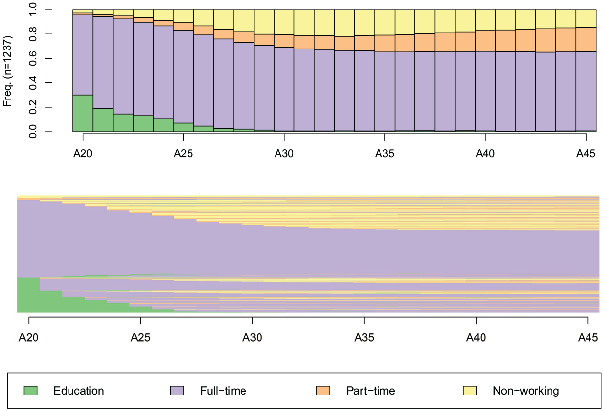
Chronogram and index plot of professional trajectories.

From Levy et al. (2006), we know that men’s trajectories are relatively homogeneous and exhibit three main phases: education, full-time work, and retirement. Women’s trajectories are much more varied, partly because of the lack of childcare services in Switzerland. Women’s average curve of working rates has a camel shape, with a decrease in working rates when children are young and a recovery thereafter. However, this average curve results from distinct types of trajectories. Some women stop working or reduce their working rates after childbirth, others return to work afterward, and some women go back and forth between work and home activities. Therefore, we can expect a strong clustering structure in the professional trajectory, distinguishing two types, one for men and one for women, or more if different types of women’s trajectories need to be characterized.

The coresidence trajectories presented in Figure 2 are coded using seven states: living with two biological parents, one parent, alone, a partner, a partner and at least one child, at least one child but no partner (i.e., a single parent), and other situations. I anticipate less structured coresidence trajectories but still centered on a few types. Previous studies show the coresidence trajectories of these cohorts are highly standardized (Levy et al. 2006) regarding the timing and sequencing of states in the trajectories.

Figure 2.

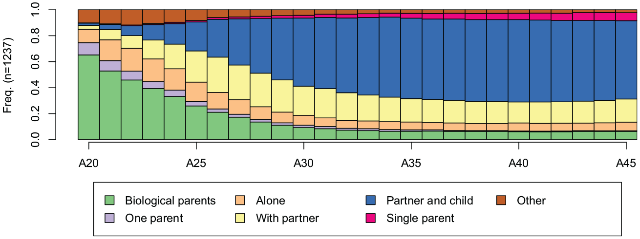
Chronogram of coresidence trajectories.

For all subsequent analyses, I use the Ward clustering algorithm without squaring distances (Batagelj 1988) and optimal matching distance with constant costs. This distance measure takes duration and sequencing into account while measuring dissimilarities between sequences (Studer and Ritschard 2016). However, the proposed procedure can be used with any clustering algorithm and distance measure. I now present the proposed method.

Parametric Bootstrap Test for Cluster Homogeneity

Hennig and Liao (2013) and Hennig and Lin (2015) proposed a new method for providing interpretation thresholds for CQIs. Building on the work of Gordon (1999), their generic framework is based on parametric bootstraps to compare the quality of the typology with that obtained by clustering similar but nonclustered data. In other words, we aim to measure the extent to which the quality of the obtained typology surpasses the one we would obtain for data with no clustering structure. If this is the case, we can be confident our typology captures a relevant clustering structure when compared with the “null case.” This comparison also provides a baseline value for interpreting CQI values and describing their behavior with a varying number of groups.

As Hennig (2015) noted, this generic framework needs to be adapted to each field of study. This adaptation requirement is a strength that guarantees the meaningfulness of the results for a specific field. In this study, I propose several adaptations of this framework to SA, each providing distinct information on the quality of the obtained clustering.

The Generic Framework

As mentioned, the general idea is to compare the quality of the obtained clustering with the quality obtained by clustering similar but nonclustered data. If the quality of our clustering falls within the range of what we usually observe for nonclustered data, we can conclude that the structure found by our clustering is weak. If our clustering quality is much higher, we can be confident and assess the relevance of our typology.

I use bootstrapping to estimate the CQI values of nonclustered data. Specifically, the parametric bootstrap procedure works by repeating n times the following operations: (1) generate similar but nonclustered data using a “null” model, (2) cluster the generated data, and (3) compute the value of the CQI of interest. The result of this bootstrap procedure is the n CQI values that we obtain by clustering the nonclustered data. We can then compare these n values with those of our clustering.

In usual statistical reasoning, these procedures allow us to estimate the null distribution of the CQI, where the null model refers to the absence of any clustering structure in the data. This strategy can overcome the lack of an independence model in cluster analysis, as we identified earlier. Following usual statistical reasoning, we use this information to derive a testlike framework to assess the clustering structure of the obtained typology.

This generic framework requires us to specify two important points. First, we need a null model to generate similar but nonclustered data. Therefore, we need to define what “similar” and “nonclustered” mean in the context of SA. As Hennig (2015) noted, there is no universal definition of the absence of a clustering structure; it should be defined according to the aims of the analysis, and this depends on the use and interpretation of the results. Second, we need to define how to measure clustering quality by choosing a CQI. However, different CQIs exist, each emphasizing a different aspect of the clustering structure (Hennig 2017).

The need to define these two points leads to the same question: what is a clustering structure? This is a sociological rather than a statistical question. Here, I propose answering it on the basis of the life-course paradigm.

Choosing a CQI

Several CQIs are available, and each measures a slightly different aspect of the statistical quality of a given typology (Hennig 2017). To choose among them, we must decide which aspects of the structure we are most interested in.

First, we need to clarify the kind of latent structure in which we are interested. Let us take the simple sociological example of Hennig and Liao (2013) to illustrate this aspect. Suppose we would like to create a typology of economic resources using income (x axis) and wealth (y axis), as shown in Figure 3.

Figure 3.

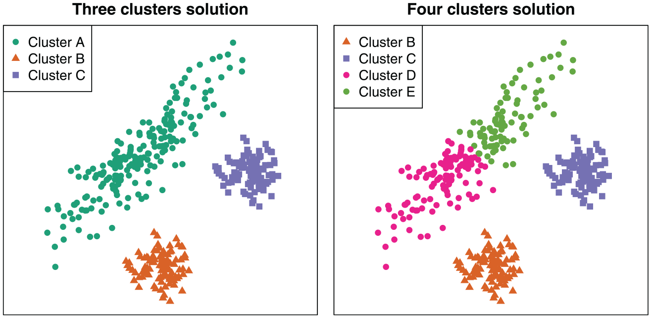
Scatterplot of the distribution of income on the x axis and wealth on the y axis for the three- and four-cluster solutions.

In this example, we can identify three groups, which are represented using different colors and symbols (see the online article for color figures). Clusters B and C seem to be homogeneous and well separated from each other; cluster A requires more discussion. If we are interested in the latent underlying structure measuring the relationship between income and wealth, cluster A is well defined, because it shows a different relationship between income and wealth than do the other two clusters. However, if we are interested in different average combinations of income and wealth, this cluster is badly defined, as it regroups different social realities. In the latter case, the four-group solution would be better.

Transposing this discussion to SA, we should decide whether we are most interested in the difference in the average trajectory or in the transition rates along these trajectories. The aim of SA is to identify frequently observed trajectories. In this sense, we are most interested in the difference in the “average” location. Latent Markov models, in contrast, would be more suited to capturing the differences in transition rates (for a review, see Piccarreta and Studer 2019).²

When building a typology focusing on different locations (i.e., “average”) between clusters, two statistical aspects could be of interest: between-cluster separation and within-cluster homogeneity. Figure 4 provides a schematic graphical representation. Between-cluster separation refers to the extent to which types differ from one another. Within-cluster homogeneity refers to the homogeneity of each type, or the extent to which each type regroups a single trajectory.

Figure 4.

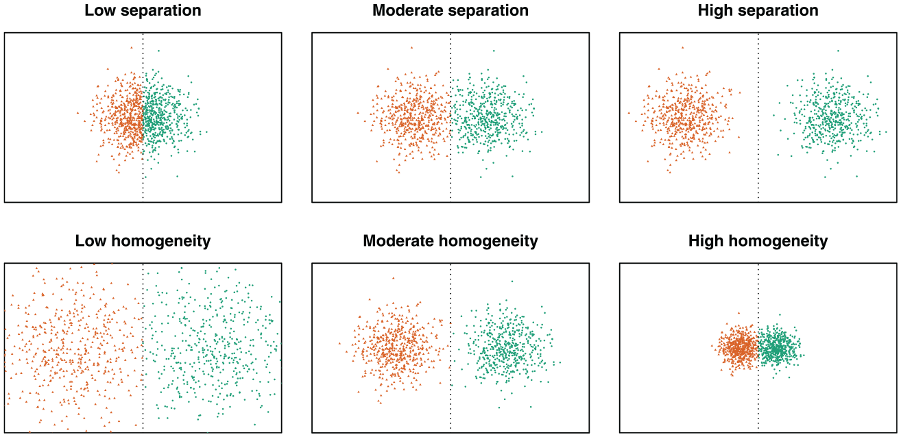
Examples of different levels of separation and homogeneity.

Separation is an important aspect when providing a structural interpretation of the resulting typology. To look for the underlying structural reasons for observing different types of trajectories, we need to observe types that are sufficiently different or well separated. Separation is also important when using the typology in subsequent analyses, such as multinomial regression, even from a descriptive perspective. Having many sequences between two types might create or hinder statistical relationships with other covariates of interest in this case (for a detailed discussion, see Studer 2013).

Yet a strong structural interpretation of the typology also requires high within-cluster homogeneity. If strong social constraints are at work, we should expect homogeneous sequences within each type. The same applies to the “trodden trail” interpretation (Shanahan 2000). Homogeneity is also important when the typology is used in subsequent analysis, because all sequences grouped into the same type are assumed to be equal in this case (for a detailed discussion, see Studer 2013).³

To conclude, we are generally interested in both aspects. Therefore, I focus here on the ASW that combines both aspects into a single index (Kaufman and Rousseeuw 1990). The ASW measures clustering quality by relating for each sequence the distances to the center of its own cluster (capturing homogeneity) to the distance to the closest other type (capturing separation). Although Kaufman and Rousseeuw (1999) provided some interpretation thresholds of ASW values, these values are only indicative, and their validity for SA is unknown. Furthermore, in many cases, the ASW index tends to favor two-group solutions (Hennig and Liao 2013).

Other indexes might be of interest. Pseudo-R² aims to measure information reduction by computing the share of the variability of the trajectories explained by the clustering (Studer et al. 2011). Researchers usually avoid this index because it lacks interpretation thresholds, even though it provides a clear interpretation. The procedure developed here provides such threshold values, so the index can be used. The same applies to the HC index, which computes the gap between the best theoretically possible clustering and the obtained one (Hubert and Levin 1976). This is among the best indexes for retrieving the correct number of groups, even though small variations should not be interpreted (Milligan and Cooper 1985). The proposed method provides a way to identify ignorable variations. Here, I focus on the ASW and HC indexes to keep the presentation simple and present a generic method.

Null Model Requirements

Aside from the choice of a CQI, we also need to define a null model. Recall that this model aims to provide a typical value of the CQI when the data should not be clustered by generating data with the null model before clustering them and computing the associated CQI.

The null model should generate similar but nonclustered data (Hennig and Lin 2015). By similar, I mean the model should reproduce the “structural features of their data sets that do not indicate clustering” (Hennig and Lin 2015:822). In most applications, some structured information should not be interpreted as a clustering structure. Therefore, this information should be reproduced by the null model. However, we should also generate nonclustered data. Data produced by the null model should not convey any information that we consider to be a clustering structure.

These two aspects require us to define the kind of structure for which we are looking. As noted earlier, this is a sociological question, not a statistical one. Here, I propose answering it on the basis of the life-course paradigm to provide a generic SA framework. This requirement has been one of the key criticisms of this framework (see the comments on Hennig and Liao 2013). Yet I regard this as one of the framework’s main strengths, as it guarantees the interpretability and usefulness of the results in specific applications (Hennig 2015).

Nonclustered Data

Generally, two broad cases of nonclustered data should lead us to avoid clustering our data. Figure 5 presents these cases schematically. First, only one type of trajectory might exist in the data. As such, any clustering would create unneeded distinctions and should be avoided. This case is uncommon in the social sciences, where individuals tend to follow diverse trajectories. Furthermore, many visualization tools are available in SA that could be used to identify it.

Figure 5.

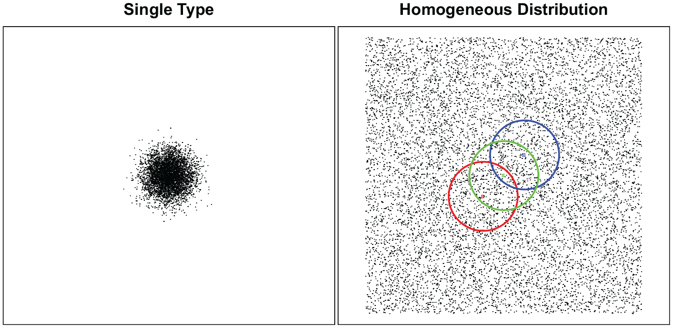
Schematic representation of homogeneously distributed data.

Second, the trajectories might be homogeneously distributed in the sequence spaces, as represented on the right-hand side of Figure 5. In this case, we have several reasons to avoid clustering the data. First, the clusters are not homogeneous or well separated, and as discussed earlier, this might raise concerns about most of the uses and interpretations of the SA typology. Second, the type assigned to a given observation is dubious. In Figure 5, blue, red, and green clustering are equally well defined; however, these regroupings might have different interpretations. The interpretation of the type of trajectory for the green point is dubious, as it depends on the choice between blue, red, and green clustering. The same reasoning could apply to any observation. Finally, in most clustering algorithms, the choice among these possibilities is not robust. Partitioning around medoids (Kaufman and Rousseeuw 1990) relies on the overall layout and, ultimately, on the borders of the sample. The bottom-up approach of many hierarchical clustering methods, such as Ward, is influenced by the small variation in pairwise distances. Thus, in all cases, the results might depend on sampling, because the cluster is not defined according to a strong regularity of the type itself.

In this study, I focus on homogeneously distributed observations for two reasons. First, this case is trickier to identify using standard descriptive and visualization tools. Second, it is common.

The null model should generate homogeneous data, but on which aspects? I base my reasoning on the life-course framework. Extending the work of Settersten and Mayer (1997) and Billari, Fürnkranz, and Prskawetz (2000), Studer and Ritschard (2016) identified three regularities of interest when using SA in life-course research.

The sequencing of states shows the path taken by individuals. This is often thought to be crucial, as many social norms or structural constraints relate to the ordering of stages in a trajectory. For instance, having a child before or after marriage is not interpreted in the same way in many countries (Hogan 1978). Sequencing also captures the dynamics of the trajectory. Observing unemployment before or after employment reveals opposite professional integration dynamics, even if the same states are observed. A recurrent ordering of the stage might also result from the steps required to access some positions.

A strong sequencing structure is found in the data when we observe only a few, but recurrent, orderings of states. In this case, a typology is an efficient way to summarize the main orderings. Homogeneous clustering is found when all paths are likely, as a sequence typology might regroup different orderings in the same types, and many sequences might lie between types.

The timing of the states or transitions (i.e., when an individual is in each state or experiences a transition) is also an important regularity in trajectories. Many studies emphasize the meaningful role of age norms over the life course (Widmer et al. 2003). Going further, Lesnard (2010) claimed that social interpretation of a state depends on when it is observed. For instance, being unemployed at age 25 or 60 has different causes and implications that should be studied on their own. Similarly, in epidemiology, the “critical period” model states that some events or states might trigger an effect only if they occur at a specific time (Kuh et al. 2003). A timing structure is found whenever some states or transitions are specific to a certain age range, or if distinct timings are found for different types.

Finally, the duration, namely, the time spent in each state or the duration of spells, is also of interest in many applications. The pattern of time spent in unemployment is a key indicator in many studies of professional integration. Spell duration also captures the relative timing, sometimes called the spacing (Settersten and Mayer 1997), between main transitions (e.g., the time between marriage and having one’s first child). In epidemiology, the concept of duration can be linked to “exposure” to a certain situation (Kuh et al. 2003). A duration structure is found when a spell in a given state typically lasts for a specific duration (e.g., when individuals tend to stay for either a long or a short time in a given type of spell, such as living alone).

These three aspects are strongly interrelated. For instance, the first and last states of a sequence partially define the timing and sequencing of a trajectory. A very long time spent in a state usually implies simpler sequencing. Therefore, it is impossible to isolate each aspect from the others. However, in many applications, understanding the specific differences stemming from each aspect is of interest, as it might lead to a more precise interpretation of the results (Studer and Ritschard 2016).

I aim to capture the clustering structure of the data arising from these three aspects. Therefore, the null model should not reproduce it. In fact, it should generate data showing the timing, sequencing, or duration as nonclustered as possible. However, it might also be of interest to measure the extent to which the data are structured according to each aspect separately.

Similar Data

The null model should reproduce any data structure that should not be interpreted as clustering. Generally, sequence data have two strongly structured characteristics that do not reflect clustering in most life-course applications.

First, and most important, trajectories are generally organized by spells (Elzinga and Studer 2015). When studying professional or family trajectories, we typically observe sequences comprising a few spells, some of them lasting for several time units. For instance, the sequence “education/4–full-time/10–inactive/6” is composed of only three spells, even if the sequence describes a trajectory of 20 years. This is a very strong structure. However, we are not particularly interested in it, because we already know about it. Therefore, our null model should also generate data organized by spells.

Second, we are rarely interested in the fact that some states or spells are more common than others. Indeed, even if there was only one type of sequence in the data (i.e., no clustering structure), we might expect different frequencies for each spell or state. For this reason, we do not consider spell or state frequency to be a structuring aspect of the sequences. Again, this means our null models should reproduce spell or state frequency, at least to some extent.

Aside from these two generic characteristics of sequence data in life-course research, one might be interested in accounting for additional nonclustering structures. Establishing a complete list is impossible, as they are mostly application specific. However, nonclustering aspects in the sequencing, timing, or duration of sequences are of special interest. Indeed, such a nonclustering structure might wrongly lead us to conclude that a significant sequencing, timing, or duration clustering structure has been found in the data.

First, some transitions might be impossible. This is generally well known, and therefore, we are not usually interested in uncovering it using a typology. For instance, when studying civil status trajectories, we know that no transition exists between divorced and single status. These impossible transitions result in regularities in the sequencing of states that should not be identified as a “clustering structure.” Therefore, it should be reproduced by our null model.

Second, some states might occur only for a predefined duration. For example, when studying school-to-work transition using monthly data, education spells typically last for a multiple of 12 months (or another fixed duration) as soon as they are observed. Here again, predefined durations might structure the data and therefore might be identified as a “clustering structure.” Reproducing it in the null model avoids such risk.

Finally, some states might occur only at predefined ages. For instance, retirement can be observed starting only from the set age of 64 years in Switzerland (without considering early retirement). This might again structure the data and result in an incorrect identification of a “timing clustering structure.”

Thus, two generic structuring aspects of sequence data should be reproduced by our null model when using SA: spell organization of the data, and state/spell frequency. I discuss three additional characteristics of sequencing (impossible transitions), duration (specific duration), and timing (specific ages). Whether these last three characteristics should be counted as a nonclustering structure is application, and even context, specific. For instance, age at first marriage, duration of education spells, and retirement age, to name just a few, can all be governed by country-specific laws. One therefore needs a careful evaluation of the type of clustering structure one aims to find in the data.

Statistical Test

The generic framework aims to provide a baseline interpretation of the CQI by computing the value obtained by clustering similar but nonclustered data. Hennig and Lin (2015) used the computed null CQI values to derive a test against clustering homogeneity in a given number of clusters. Let m be the number of bootstraps, k the number of clusters, $x_{0, k}$ the observed CQI values for the clustering in k groups, and $x_{i, k}$ the CQI of the ith bootstrap. Then, the p value is estimated using

{\hat{P}}_{k} = \frac{\sum_{i}^{m} I (x_{i, k} \geq x_{0, k}) + 1}{m + 1},

where $I (\cdot)$ is the indicator function.

In a standard application, ${\hat{P}}_{k}$ is typically evaluated for a varying number of clusters k. This might imply a high number of tests, and therefore, we need to account for multiple testing. I propose to do so by using the “Max T” approach (Westfall and Troendle 2008; Westfall and Young 1993).⁴ The “Max T” approach estimates a single null distribution of the test statistics by recording, for each bootstrap, the maximum value of this statistic among the different number of groups k. By doing so, the null distribution accounts for multiple testing and correlations between the tests (Westfall and Young 1993).⁵

Looking at the maximum of the CQI values is meaningful only if these CQI values are comparable for different numbers of groups k. Hennig and Lin (2015) proposed improving the comparability of these values by standardizing them using the average and standard deviation of the null distribution of the CQI for a given number of groups k. Romano and Wolf (2005) also advocated this approach in their more general discussion on the “Max T” approach.

As a result, we can distinguish three approaches to build a statistical test against cluster homogeneity. First, the p values might be computed for a given number of groups. Second, a general test can be computed, accounting for multiple testing, using the “Max T” approach either with or without standardization. In this study, I present all these approaches, as they might be useful in some applications. However, I favor the standardized “Max T” approach, as it controls for multiple testing and does not assume CQI values are comparable across different numbers of groups. I now turn to the null models and show more practically the differences between these approaches.

Null Models for Sequence Analysis

Earlier, I presented several properties that should be fulfilled by the null model. In life-course research, we are interested in capturing the structure stemming from sequencing, timing, and duration, either globally or in the specific structure in each aspect. At the same time, we would like to avoid taking into account the spell organization of sequences and the state or spell frequencies. In some applications, we would also like to consider impossible transitions, specific duration, and ages as nonclustering structures. Finally, the null model depends on the aim of the analysis. In this section, I present five null models for SA, each following a different goal and providing different information.

I start by discussing three spell-based null models that aim to reproduce the spell organization of sequences, before presenting a state independence model, a model generating sequence position by position, and a transition rate–based model. All these models are complementary, as each provides specific information on the type of clustering structure revealed (or not) by the created typology.

Spell-Based Null Models

Sequences in the social sciences are generally organized by spells and can be represented as such (Elzinga and Studer 2015). For example, the professional trajectory of a woman working full-time (F) for 5 years before working part-time (P) for 20 years is usually represented as a sequence of 25 positions, such as

\underset{5}{\underset{︸}{FF \dots F}} \underset{20}{\underset{︸}{PP \dots P \dots P}} .

(1)

However, it can also be represented as a spell sequence in the form $(F, 5) (P, 20)$ . In the latter case, the sequence is described by a state vector $x = (F, P)$ and an attached duration vector $t = (5, 20)$ . Such a representation emphasizes two dimensions of the sequences: the sequencing of the state (state vector) and the time spent in each state (duration vector). Contrary to the usual representation of sequences, the timing dimension is downgraded.

Using this spell representation, we can create sequence data by generating two vectors, one for the states and another for the durations, emphasizing sequencing and duration. By doing so, we reproduce one of the strongest regularities in the sequences used in the social sciences, its organization by spells.

I propose three models, each providing specific information on the quality of the obtained typology. Whereas “randomized sequencing” measures the added value of the typology compared with the situation in which all paths are likely, “randomized duration” measures the captured structure in the data that results from the time spent in each state. Finally, the first model presented, “combined randomization,” combines these two dimensions.

Combined Randomization

Following the spell representation of sequences presented earlier, I create two vectors for each sequence. The state vector is created by sampling states among all the spells. To avoid impossible transitions, I use the following procedure. I start by randomly sampling the first state. The next states are sampled among possible states given the previous one. In all cases, the sampling is weighted by the relative frequencies of states among all possible spells. The sequencing is as random as possible, although the spell frequency of the original data is maintained.

The duration vector is created by sampling duration among all the observed spells. Because we do not attach duration to the state, the durations are completely random, even if they are typically observed in the data. If our sequences are generally composed of long spells, this will be reproduced by the null model. This procedure can easily be extended to account for the specific spell duration in some states (e.g., multiple of 6 or 12). Finally, the sequences are cut to match the observed length in the data.⁶

This null model reproduces the spell structure of sequences and a spell state’s frequencies and durations, while randomizing sequencing, duration, and, as a result, timing. Figure 6 presents the sequences generated using this null model for professional career data. The chronogram shows the sequences generated among all bootstraps, and the index plot represents only one bootstrap to avoid overplotting. As expected, timing, duration, and sequencing are not reproduced, but the spell organization of sequences is. The state frequency at each time point is not reproduced because the durations are not attached to states. Nonetheless, the full-time (violet) state is still the most frequent.

Figure 6.

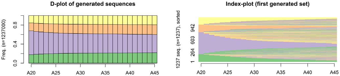
Chronogram and index plot of some of the sequences generated by the combined randomization null model.

As a reminder, the aim of this procedure is to generate sequences, cluster them, and compute the CQI. These CQI values are then recorded and used to provide a baseline value for the CQI of our own clustering. The clustering algorithm and distance measures should be the same as in our original analysis. Figure 7 shows two density plots of this null distribution for clustering between 2 and 10 clusters. The plot on the left presents the null distribution of the raw CQI values using the “Max T” approach. The colored area under the curve represents the 95 percent observed interval of these values. The values obtained in the original data are represented using a vertical black line labeled with the number of groups.

Figure 7.

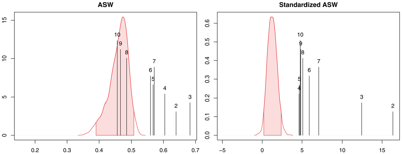
Distribution of the raw and standardized ASW null values for 2 to 10 clusters using the “Max T” approach.

The central 95 percent ASW values lie in the interval $[0.39; 0.51]$ according to the “Max T.” This interval is close to the inconclusive interval $[0.25; 0.5]$ proposed by Kaufman and Rousseeuw (1990). However, this is application specific. For the coresidence trajectory, the bootstrapped 95 percent “Max T” interval is $[0.29; 0.37]$ , which is below these standard values. This result illustrates it is not possible to define generic CQI value thresholds, thereby calling for the proposed framework.

By construction, any ASW value in the 95 percent interval $[0.39; 0.51]$ is comparable with a situation in which no clustering structure exists. Therefore, we can exclude the solutions in 8 to 10 groups. The ASW values obtained with two to seven groups are well outside this range. Therefore, we can consider that they reveal a clustering structure in the data. Following the testlike interpretation of the results presented in the “Statistical Test” section, we can reject the assumption of our null model on the basis of our data of homogeneous sequencing and spell durations. Thus, our typology reveals a timing, duration, or sequencing structure if we consider two to seven groups.

The right-hand plot of Figure 7 presents the same null distributions for the standardized value of the CQI (ASW). Recall that the aim of standardization is to account for the changing behavior of the CQI measure and clustering algorithm for a different number of clusters. A high standardized value can then be interpreted as a high relative gain in the structure found for a given number of groups. Using standardized values leads to slightly different conclusions, as all numbers of groups are flagged as significant.

We can also examine the null CQI according to the number of groups. Following the presentation proposed by Hennig and Lin (2015), the left-hand side of Figure 8 presents the ASW of our typology for a varying number of groups using a solid black line. The 1,000 bootstrapped CQI values are represented with individual gray lines, and a 95 percent interval is computed and represented using a gray polygon. The horizontal red dotted line shows the upper bound of the null confidence interval using the “Max T” approach. The right-hand side of the figure represents the standardized ASW values. According to this analysis, the two- or three-group solutions seem particularly well suited. If we want to favor a larger number of groups, the seven-cluster solution seems to be a good compromise.

Figure 8.

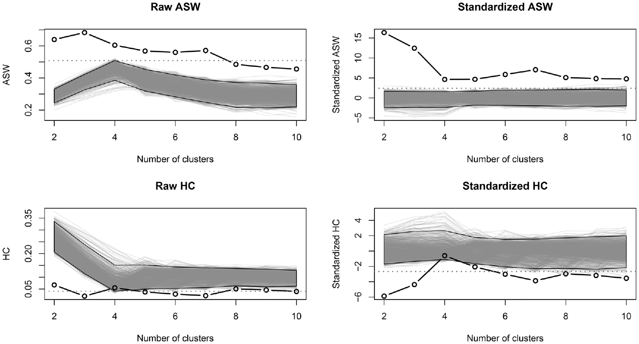
Observed and bootstrapped values of the ASW and HC values for a varying number of clusters using the combined (sequencing and duration) randomization null model.

Figure 8 also describes the evolution of the CQI with a varying number of groups when no clustering should be found in the data. In this case, we tend to observe the highest ASW values with four groups corresponding to the number of states in the alphabet.

This visualization is of special interest when using a CQI that cannot be directly compared for a different number of groups, such as pseudo-R² or the HC index. Recall that the HC index, which should be minimized, is among the best indexes for selecting the correct number of groups, according to Milligan and Cooper (1985), if small decreases are not taken into account. The proposed procedure allows us to consider the expected decrease. Figure 8 also presents the bootstrapped and observed values of the HC index, which leads us to consider the same number of groups (i.e., two, three, or seven).

Randomized Sequencing

The previously introduced null model is generic, as timing, duration, and sequencing are randomized. Here, I propose focusing on sequencing and measuring the clustering structure arising from the ordering of the state. We achieve this by randomly generating the state vector using the same procedure as for the previously presented “combined” approach. However, the durations are sampled among the spell of a given state. Here, again, the sequences are cut to match the observed length in the data. Under such a strategy, the sequencing is completely randomized, but the time spent in each state is maintained as in the original data. As a result, any duration clustering structure (i.e., specific duration) is taken into account. Comparing this clustering with that obtained by randomized sequencing, we can measure the differences in the structured sequencing in the data.

Figure 9 presents a chronogram of the sequences generated among all bootstraps and an index plot of one of the generated data sets. The generated sequences are likely, in the sense they could have been observed. The frequencies of each state are reproduced, but the timing is not.

Figure 9.

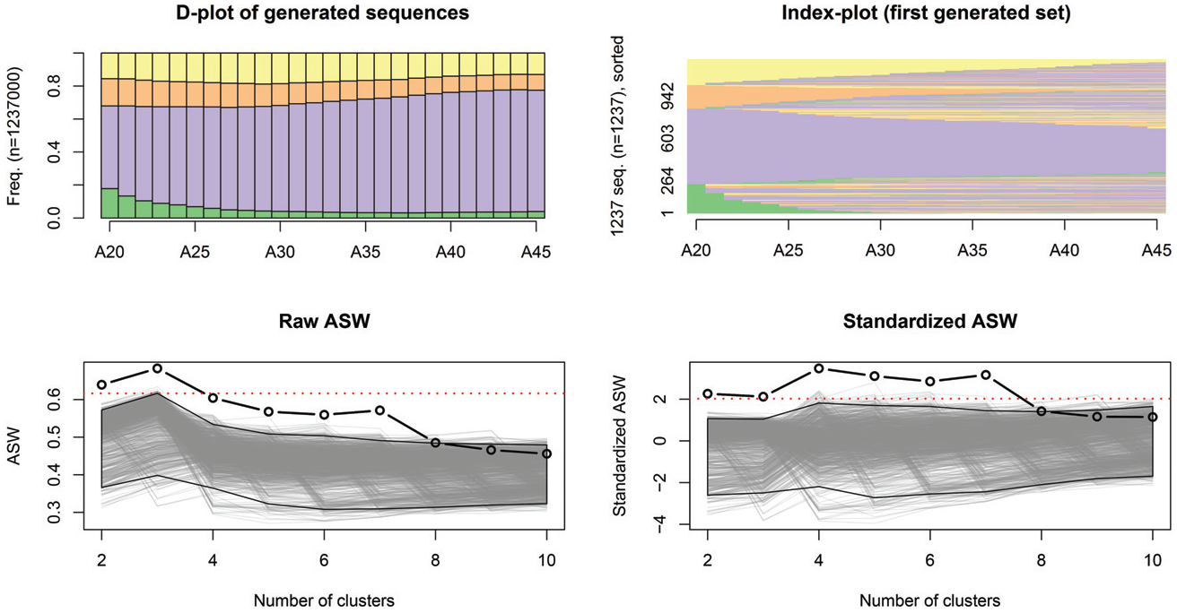
Randomized sequencing simulation results.

Figure 9 also presents the bootstrapped and observed ASW values for the number of clusters. The observed ASW values are higher than the null values with fewer than eight groups, meaning our typology reveals a structured state’s ordering in the sequences. The highest “relative” gain is found for the four- and seven-cluster solutions if we examine the normalized ASW. Further interpretations can be drawn by comparing these results with the combined randomization ones, which favor two- or three-group solutions. Because this is not the case for “randomized sequencing,” it means the structures identified for two or three groups mostly relate to the time spent in each state.

Randomized Duration

Instead of focusing on sequencing, I focus here on duration. I generate sequences by keeping the same observed sequencing but randomizing the associated duration in each state. To do so, I randomly draw a proportion of the trajectory spent in each state using a uniform distribution. By keeping the same ordering, “impossible transitions” are automatically taken into account. This strategy allows us to measure the structure arising from the duration in sequences comprising more than one spell, but sequences with only one spell are fully reproduced. Indeed, the proportion of time spent when there is only one spell must be 100 percent.

Figure 10 presents a chronogram and an index plot of some of the sequences generated using this null model. The sequences could have been observed, but we observe sequences with a long time spent in education, which is unlikely. As expected, the sequences in full-time employment are fully reproduced, and therefore are counted as nonclustering structure of the data.

Figure 10.

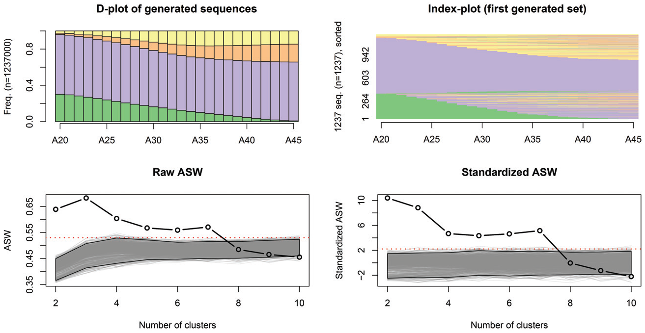
Randomized duration simulation results.

As before, Figure 10 presents the observed and bootstrapped ASW values for our typology. We observe a high value of the bootstrapped CQI for the four-cluster solution (i.e., one cluster for each possible state in the sequences). This is probably because a clustering solution according to the dominant state in each sequence tends to be a good one. According to this null model, there is no added value of going beyond eight groups. Confirming our previous interpretation, we see a high relative gain (i.e., standardized value) for two- and three-cluster solutions, which should, therefore, be primarily linked to the time spent in each state.

Position-Based Null Models

Sequences can also be generated position by position using transition rates. Starting from a given first state, the sequences are then built position by position by examining the previous state. Technically, a very general framework can be defined by using a time-dependent transition matrix. Such a matrix typically allows one to take into account impossible transitions (by setting the corresponding transition rate to zero) or age-specific states, such as retirement. Therefore, all position-based null models can consider these two aspects as nonclustering structures.

This solution is appealing, as it is possible to reproduce many timing, sequencing, and duration structures depending on the transition matrix. However, two objections can be made. First, as I already argued, we are not interested in the difference in the relationships between variables, such as transition rates, but in the difference in the “average” observed sequence. Second, a transition matrix is not necessarily a good candidate for a null model, as it might reproduce many kinds of clustering structures of the data. This can be exemplified using the following transition matrix:

[\begin{matrix} A & B & C \\ A & 0 & . 5 & . 5 \\ B & 0 & 1 & 0 \\ C & 0 & 0 & 1 \end{matrix}] .

Additionally, suppose all sequences start in state A. With such a transition matrix, we would end up with two observed sequences: a sequence with the pattern $AB \dots B$ and another with $AC \dots C$ . As a result, the observed sequences are strongly structured in two groups, even if we use a single transition matrix. Therefore, we need to choose a suitable transition matrix. Hennig and Lin (2015) used time-varying observed transition rates. However, with such a number of parameters, we can almost fully reproduce the original data, including its potential clustering structure. I tested this option and found the observed CQI always lies in the confidence interval of the bootstrapped CQI values.⁷

The question, therefore, is which transition matrix to use. I investigate two possibilities, each corresponding to a model-based approach. First, I discuss the state independence model, which is strongly related to the underlying assumptions of latent class analysis (Piccarreta and Studer 2019). Second, I discuss the use of homogeneous transition rates, an assumption underlying certain (hidden) Markov models (Piccarreta and Studer 2019). However, as already mentioned, the framework is very generic and can easily be adapted for specific applications.

State Independence

In the state independence model, the state at a given position is independent of the previous one. To recognize the basic properties of the data, the state distribution at each time point is respected. Technically, this can be simply achieved using the time-varying distributions of the states, independently of the previous state, in our time-varying transition matrix. By definition, this procedure considers any age-specific state as a nonclustering structure. This null model is roughly equivalent to the conditional state independence assumption that underlies latent class analysis.

Figure 11 presents a chronogram and an index plot of some of the sequences generated using this null model. The chronogram seems plausible with the time-varying state distribution perfectly reproduced, but the index plot presents many sequences we would never observe in the social sciences, with far too many transitions. Therefore, the spell organization of the observed sequences is not reproduced by the model.

Figure 11.

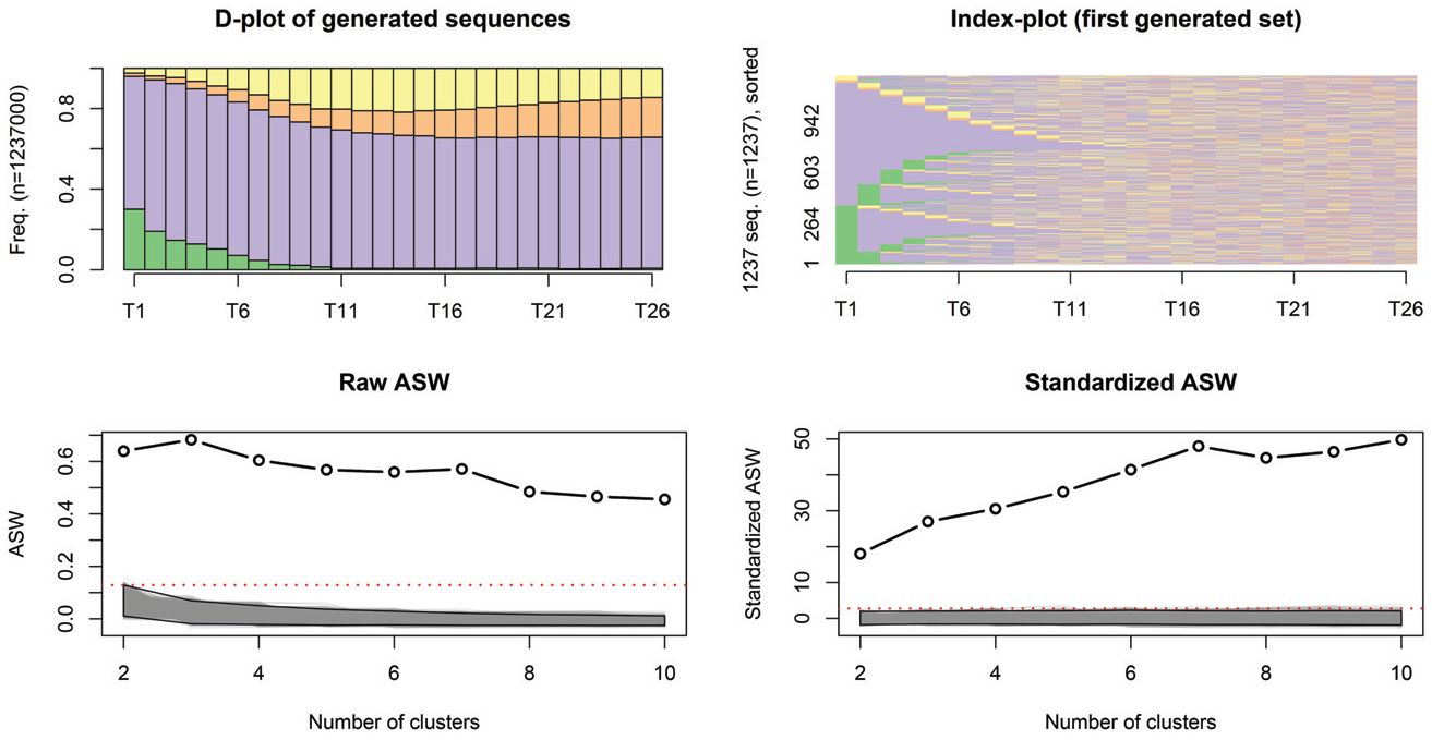
State independence simulation results.

As a result, the bootstrapped CQI values are low and decreasing (see Figure 11). We always find a significant clustering structure in the data. However, this is most likely related to the spell structure of the sequences in the social sciences, which is not respected here. Therefore, I do not recommend it for testlike interpretations. Nonetheless, it might be useful to guide the choice of the number of groups. The standardized CQI indicates a solution in 7 or 10 groups.

First-Order Markov Null Model

In the first-order Markov null model, we use the time-homogeneous transition rates. These transition rates are computed over the whole sequence, independently of the position. This is often called a Markov assumption, where the state depends only on the previous one.

More formally, the transition rate $p (b | a)$ between states a and b is estimated using the formulae given in Gabadinho et al. (2011). Let $N (a_{t})$ be the number of times we observe state a at time t and any state at time t+1. Let $N (a_{t}, b_{t + 1})$ be the number of times we observe state a at time t and state b at t+1. Then,

p (b | a) = \frac{\sum_{t = 1}^{L - 1} N (a_{t}, b_{t + 1})}{\sum_{t = 1}^{L - 1} N (a_{t})},

with $L$ the maximal observed sequence length.

We then generate the sequence by randomly selecting the first state in the sequence according to the observed proportion of each state at time one. The rest of the sequence is then generated position by position using the time-homogeneous transition rates. Therefore, this null model considers impossible transition as a nonclustering structure by definition.

Under the life-course paradigm, the notion of timing can refer to either the states within the process, as discussed earlier or the timing of the transitions between states. Using a first-order Markov null model, we assume the transition rates are not time varying. Therefore, in our framework, a strong structure would be found if the timing of transitions differed among clusters.

Figure 12 presents a chronogram of all the generated sequences and an index plot of one of the generated data sets. The generated sequences are similar to the observed ones, except we see less transition out of full-time employment at the beginning of the sequences and more at the end. As a result of this similarity, the observed ASW is not much higher than the bootstrapped ones (see Figure 12). Here, the highest standardized value is found for the seven-cluster solution. This leads us to think the seven-cluster solution captures significant structured timing in the data.

Figure 12.

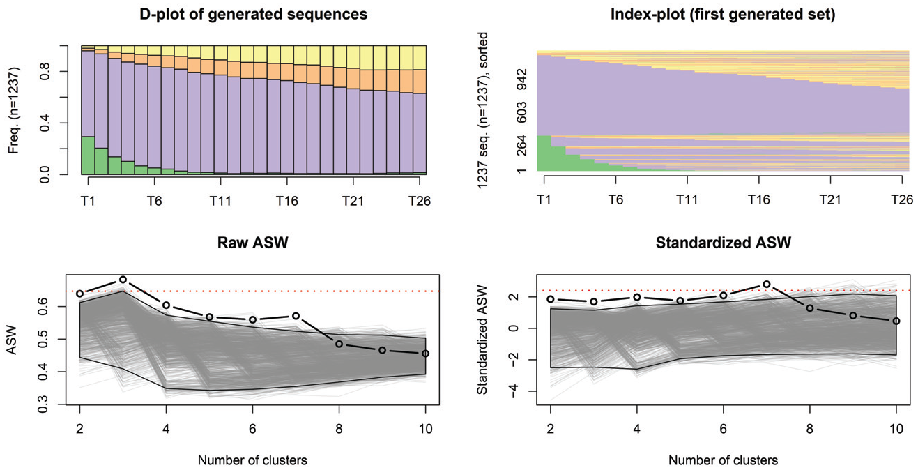
First-order Markov null model simulation results.

Choosing a Null Model

So far, I have presented five null models centered around the three central aspects of trajectories for life-course research: sequencing, duration, and timing. In this subsection, I take a broader perspective and discuss their added value and typical uses. I highlight how their results complement each other and how they could be used simultaneously to make a better informed choice.

Let us start by recalling their main properties, as summarized in Table 1. The first three columns present the clustering structure of the sequence data the null models aim to capture—sequencing, timing, and duration. The next four columns show the nonclustering structure reproduced by the null model, which is therefore not counted as clustering (see the “Similar Data” subsection). In these columns, a check mark in parentheses denotes an aspect that can optionally be reproduced by the model.

Table 1.

Main Properties of the Null Models.

	Clustering Structure			Nonclustering Structure
Null Model	Sequence	Duration	Timing	Spell	Impossible Transitions	Specific Duration	Specific Age
Spell-based models
Combined randomization	✓	✓	✓	✓	(✓)^c	(✓)^c
Randomized sequencing	✓		✓^a	✓	(✓)^c	✓
Randomized duration			✓^a	✓	✓
Position-based models
State independence	✓	✓			(✓)^c		✓
First-order Markov model			✓^b	✓	✓		(✓)^c

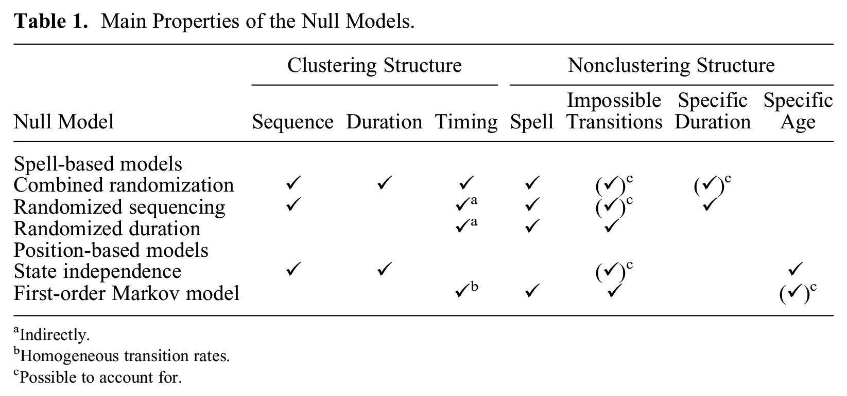
Indirectly.

Homogeneous transition rates.

Possible to account for.

The “combined” model randomizes the duration and the sequencing of the states, and therefore, their timing as well. Impossible transitions or specific durations can optionally be taken into account. It is a generic null model reproducing the structuration of sequences in spells.

The “sequencing” null model randomizes the sequencing of the states while maintaining spell duration (and therefore, specific durations). As a consequence, this null model also randomizes, although to a lesser extent, the timing of the state and transitions. Impossible transitions can be considered.

The “duration” null model retains the original sequencing of the data (and therefore, impossible transition) but randomizes the duration vectors, and, to a lesser extent, the timing of the states. As discussed, this null model is less well suited when many individuals stay in the same single state for the whole sequence, because these sequences are not randomized. For this reason, this null model should be primarily used when such sequences are infrequent.

The “state independence” model reproduces the sequence position by position while randomizing their sequencing and durations. Impossible transitions can be taken into account. Because it does not reproduce the spell structure of the sequences, it might generate highly unlikely sequences for most life-course research applications. Therefore, this null model should be used with caution.

In our example, the “first-order Markov model” produced the most similar sequences for every aspect except the time-varying transition rates. Age-specific states can be taken into account if needed. It is a reasonable null model when we are interested in the timing structure of transitions within the sequences. However, as discussed in the “Position-Based Null Models” section, models based on transition rates might produce highly clustered data. Therefore, I recommend closely examining the transition rates before using it.

Having five null models implies making a choice. I propose to do so on the basis of the research questions and data characteristics. For some research questions, one of the three aspects of sequencing, timing, or duration are of primary interest. For instance, in their study of professional integration of people who reach the end of unemployment benefits, Studer, Hadziabdic, and Ritschard (2015) focused on the ordering of social policies and their possible consequences. In these situations, null models that randomize the primary aspect of interest should be favored.

The characteristics of the data should also be considered. In some applications, one of these three aspects might vary only slightly between observations. In this case, null models focusing on the randomization of this specific aspect are irrelevant. Indeed, the baseline would be the maximal variation of this aspect. For instance, Gabadinho and Ritschard (2013) studied sequences of childbirth histories where the states were defined using women’s parity at a given age. Here, the ordering of the state is almost constant, as having two children can only follow having one (or zero in the case of twins). There would be almost no interest in comparing our clustering with the situation in which all orderings are possible.

The proposed null models randomize each aspect as much as possible. This has several advantages. First, they are generic and can be used in most applications. Second, they provide a common baseline across applications. Finally, because they are generic, they can be made readily available in statistical software, and it is in the WeightedCluster R library (Studer 2013).

However, in some applications, it might be beneficial to take into account additional nonclustering structures of the data by adapting the null models. This is particularly useful in a testlike interpretation of the result, as the corresponding null model fully accounts for the specificity of the data. Aside from the spell structure of the data and spell (or state) frequencies, several application-specific aspects might be taken into account, namely, impossible transitions, specific durations, and specific ages. For instance, in a study of lifelong professional careers, one might want to account for the nonclustering structure of the timing of retirement, that is, the fact that retirement cannot occur at the beginning of the trajectory. In these situations, a strict testlike interpretation of the generic null model result is at risk of detecting a “significant” clustering structure, precisely because of the nonclustering structure of age at retirement. Therefore, specifying these nonclustering structures in the null models that can handle them is recommended. In some cases, it might even be necessary to adapt the null models further or to develop a new one. However, the generic null models should provide useful baseline values for the CQI for most applications, as long as interpretation of the results takes this nonclustering structure into account.

In summary, the choice of a null model should be grounded in the research question and the data at hand. Some aspects might not be of primary interest, and therefore their associated null models would not bring any relevant information. However, most of the time, we are interested in the three aspects taken together. In this situation, I suggest using all the null models, as they might each illustrate some of the strengths and weaknesses of each clustering solution.

Let us illustrate this by summarizing the results of our empirical example. Generally, clustering between two and seven groups is found to be significant by all null models, except the “first-order Markov,” which flags only the seven-cluster solution. We can also look at the number of groups favored by each null model. The “combined” and “duration” null models, which both randomize duration, opt for the two- and three-cluster solutions. The “sequencing,”“first-order Markov,” and “state independence” model, which randomize timing and sequencing, lead to the choice of the seven-cluster solution. This last solution is also the third “choice” of the “combined” null model.

Figure 13, which presents the three- and seven-cluster solutions, confirms this interpretation. The three-cluster solution mainly distinguishes the patterns according to the overall time spent in the three most frequent states: full-time, part-time, and nonworking. The seven-cluster solution makes further distinctions according to timing and sequencing. For instance, clusters 3 and 4 distinguish the timing of the transition between full-time and part-time employment. A similar distinction is found between clusters 2 and 6. Clusters 6 and 7 make a distinction according to the sequencing of the states by separating individuals going back to part-time employment.

Figure 13.

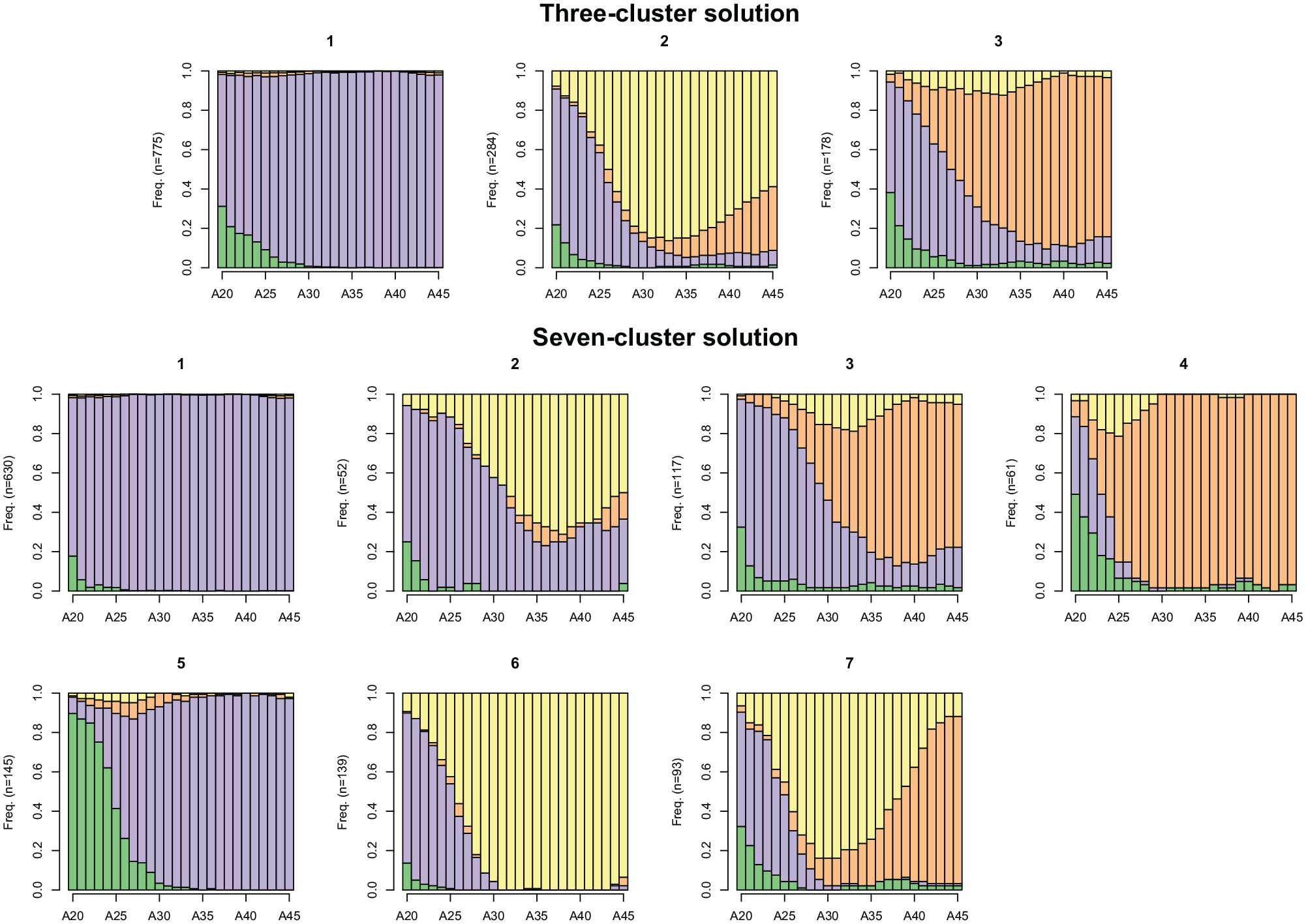
Final typologies of professional trajectories in Switzerland.

Comparison of the results across null models provides useful information on the type of structure identified by the observed typology. Here, they all lead to the same conclusion that a significant timing, duration, or sequencing structure is found in the data. However, such interpretation requires some caution, as it implies multiple testing. This is particularly true if only one of the null models provides significant results, as one would generally expect an agreement between some of these tests because they are, by construction, highly correlated.

The ultimate choice between all these solutions should not be based on statistical criteria. These solutions are validated by the proposed procedure as were all the cluster solutions with fewer than eight groups. The choice should be made according to the application and theories being tested. Is it worth having seven categories representing professional trajectories? Should we distinguish according to timing and sequencing, or mainly the time spent in each state? The aim of the validation procedure is to avoid drawing wrong conclusions about the structure of the data and not to replace the theory of the domain under study.

Conclusion

In this study, I proposed a method for the validation of SA typologies on the basis of parametric bootstraps. The method works by comparing the quality of the obtained clustering with the quality obtained by clustering similar but nonclustered data. If the quality of our clustering lies in the range of what we usually observe for nonclustered data, we can conclude that the structure captured by our clustering is weak. If our clustering quality is higher, our typology identifies a relevant clustering structure.

To use the framework, we need a null model to generate similar but nonclustered data. I proposed five null models to test the different structuring aspects of the sequences important in life-course research, namely, sequencing, timing, and duration. The use of parametric bootstrap provides the expected behavior of CQIs for different types of structures. It offers a better interpretation of clustering quality and the type of structure found in the data. It also supports a testlike interpretation. Finally, the proposition of several specific null models forces us to think about the kind of structure we are looking for in the data. This is one of the key strengths of the generic framework proposed by Hennig and Lin (2015). This question should be answered on the basis of social science arguments and therefore will always be application specific. However, the proposed null models provide some directions for thinking about it on the basis of the life-course paradigm.

The proposed methods are a great addition to SA. It is a first step toward an integrated approach for the evaluation and validation of SA typologies. The lack of a suitable methodology is among the long held criticisms of SA. However, a typology might be useful even if it is not validated by the proposed method. As Hennig and Lin (2015) pointed out, in some applications, there is a need to reduce the information into a few types, even if it does not reveal a clustering structure of the data. However, even in this case, the proposed method provides useful information by revealing that no clustering structure has been found according to the tested dimensions.

The proposed method focuses on two aspects of the validation of a typology from a statistical perspective, namely, within-cluster homogeneity and between-cluster separation. However, other aspects are also important. Han, Liefbroer, and Elzinga (2017) stressed that a good typology should reproduce known associations with other key variables, such as education and gender. Hennig (2007, 2008) emphasized the stability of clustering across several samples. Finally, many studies stress the importance of the interpretability and theoretical soundness of the results (see, e.g., Piccarreta and Studer 2019). All these aspects are important and should be considered. However, we still lack a well-defined integrated approach to do so. This is probably one of the most important challenges facing SA.

Footnotes

Acknowledgements

I would like to thank the anonymous reviewers for their careful reading and their insightful comments and suggestions. I also gratefully acknowledge benefiting from the support of the Swiss National Centre of Competence in Research LIVES’s Overcoming Vulnerability: Life Course Perspectives (NCCR LIVES), which is financed by the Swiss National Science Foundation (grant 51NF40-160590).

ORCID iD

Matthias Studer

Notes

Author Biography

Matthias Studer is an associate professor in the Faculty of Social Sciences of the University of Geneva and at the LIVES Centre. His research interests include sequence analysis, gendered career inequalities, and labor market studies and social policy evaluation. He is one of the developers of the TraMineR R library and the maintainer of the WeightedCluster R library, both for sequence analysis. He recently published on time-varying covariates in sequence analysis in Sociological Methodology, on discrepancy analysis in Sociological Methods & Research, and a comparison of sequence analysis distance measures in the Journal of the Royal Statistical Society: Series A.

References

Abbott

Andrew

. 1995. “Sequence Analysis: New Methods for Old Ideas.” Annual Review of Sociology 21:93–113.

Abbott

Andrew

. 2000. “Reply to Levine and Wu.” Sociological Methods & Research 29(1):65–76.

Abbott

Andrew

Forrest

John

. 1986. “Optimal Matching Methods for Historical Sequences.” Journal of Interdisciplinary History 16(3):471–94.

Abbott

Andrew

Hrycak

Alexandra

. 1990. “Measuring Resemblance in Sequence Data: An Optimal Matching Analysis of Musician’s Careers.” American Journal of Sociology 96(1):144–85.

Abbott

Andrew

Tsay

Angela

. 2000. “Sequence Analysis and Optimal Matching Methods in Sociology, Review and Prospect.” Sociological Methods and Research 29(1):3–33.

Batagelj

Vladimir

. 1988. “Generalized Ward and Related Clustering Problems.” Pp. 67–74 in Classification and Related Methods of Data Analysis, edited by Bock

H. H.

Amsterdam, the Netherlands: North-Holland.

Bernardi

Laura

Huinink

Johannes

Settersten

Richard A.

2019. “The Life Course Cube: A Tool for Studying Lives.” Advances in Life Course Research 41:100258.

Billari

Francesco C.

Fürnkranz

Johannes

Prskawetz

Alexia

. 2000. “Timing, Sequencing, and Quantum of Life Course Events: A Machine Learning Approach.” Working Paper 010. Rostock, Germany: Max Planck Institute for Demographic Research.

Brückner

Hannah

Mayer

Karl Ulrich

. 2005. “De-standardization of the Life Course: What It Might Mean? And if It Means Anything, Whether It Actually Took Place?” Advances in Life Course Research 9(1):27–53.

10.

Brzinsky-Fay

Christian

. 2014. “The Measurement of School-to-Work Transitions as Processes.” European Societies 16(2):213–32.

11.

Elzinga

Cees H.

Studer

Matthias

. 2015. “Spell Sequences, State Proximities and Distance Metrics.” Sociological Methods and Research 44(1):3–47.

12.

Gabadinho

Alexis

Ritschard

Gilbert

. 2013. “Searching for Typical Life Trajectories Applied to Childbirth Histories.” Pp. 287–312 in Gendered Life Courses: Between Individualization and Standardization, A European Approach Applied to Switzerland, edited by Levy

Widmer

Vienna, Austria: LIT-Verlag.

13.

Gabadinho

Alexis

Ritschard

Gilbert

Müller

Nicolas S.

Studer

Matthias

. 2011. “Analyzing and Visualizing State Sequences in R with TraMineR.” Journal of Statistical Software 40(1):1–37.

14.

Gordon

A. D.

1999. Classification. New York: Chapman & Hall/CRC.

15.

Han

Liefbroer

Aart

Elzinga

Cees

. 2017. “Comparing Methods of Classifying Life Courses: Sequence Analysis and Latent Class Analysis.” Longitudinal and Life Course Studies 8(4):319–41.

16.

Hennig

Christian

. 2007. “Cluster-Wise Assessment of Cluster Stability.” Computational Statistics and Data Analysis 52(1):258–71.

17.

Hennig

Christian

. 2008. “Dissolution Point and Isolation Robustness: Robustness Criteria for General Cluster Analysis Methods.” Journal of Multivariate Analysis 99(6):1154–76.

18.

Hennig

Christian

. 2015. “What Are the True Clusters?” Pattern Recognition Letters 64(1):53–62.

19.

Hennig

Christian

. 2017. “Cluster Validation by Measurement of Clustering Characteristics Relevant to the User.” arXiv. Retrieved April 30, 2021. https://arxiv.org/abs/1703.09282.

20.

Hennig

Christian

Liao

Tim F.

2013. “How to Find an Appropriate Clustering for Mixed-Type Variables with Application to Socio-economic Stratification.” Journal of the Royal Statistical Society: Series C (Applied Statistics) 62(3):309–69.

21.

Hennig

Christian

Lin

Chien-Ju

. 2015. “Flexible Parametric Bootstrap for Testing Homogeneity against Clustering and Assessing the Number of Clusters.” Statistics and Computing 25(4):821–33.

22.

Hennig

Christian

Meila

Merina

Murtagh

Fionn

Rocci

Roberto

, eds. 2015. Handbook of Cluster Analysis. New York: Chapman & Hall/CRC.

23.

Hogan

Dennis P.

1978. “The Variable Order of Events in the Life Course.” American Sociological Review 43(4):573–86.

24.

Hubert

Lawrence J.

Levin

Joel R.

1976. “A General Statistical Framework for Assessing Categorical Clustering in Free Recall.” Psychological Bulletin 83(6):1072–80.

25.

Kaufman

Leonard

Rousseeuw

Peter J.

1990. Finding Groups in Data: An Introduction to Cluster Analysis. New York: John Wiley.

26.

Kuh

Ben-Shlomo

Lynch

Hallqvist

Power

2003. “Life Course Epidemiology.” Journal of Epidemiology & Community Health 57(10):778–83.

27.

Lesnard

Laurent

. 2010. “Setting Cost in Optimal Matching to Uncover Contemporaneous Socio-temporal Patterns.” Sociological Methods and Research 38(3):389–419.

28.

Levine

J. H.

2000. “But What Have You Done for Us Lately.” Sociological Methods & Research 29(1):35–40.

29.

Levy

René

Gauthier

Jacques-Antoine

Widmer

Eric

. 2006. “Entre Contraintes Institutionnelle et Domestique: Les Parcours de vie Masculins et Féminins en Suisse.” Cahiers Canadiens de Sociologie 31(4):461–89.

30.

Liefbroer

Aart C.

Toulemon

Laurent

. 2010. “Demographic Perspectives on the Transition to Adulthood: An Introduction.” Advances in Life Course Research 15(1):53–58.

31.

Mayer

Karl Ulrich

. 2009. “New Directions in Life Course Research.” Annual Review of Sociology 35:413–33.

32.

Milligan

Glenn

Cooper

Martha

. 1985. “An Examination of Procedures for Determining the Number of Clusters in a Data Set.” Psychometrika 50(2):159–79.

33.

Piccarreta

Raffaella

Studer

Matthias

. 2019. “Holistic Analysis of the Life Course: Methodological Challenges and New Perspectives.” Advances in Life Course Research 41:100251.

34.

Romano

Joseph P.

Wolf

Michael

. 2005. “Stepwise Multiple Testing as Formalized Data Snooping.” Econometrica 73(4):1237–82

35.

Settersten

Richard A.

Jr. Mayer

Karl Ulrich

. 1997. “The Measurement of Age, Age Structuring, and the Life Course.” Annual Review of Sociology 23:233–61.

36.

Shanahan

Michael J.

2000. “Pathways to Adulthood in Changing Societies: Variability and Mechanisms in Life Course Perspective.” Annual Review of Sociology 26:667–92.

37.

Studer

Matthias

. 2013. “WeightedCluster Library Manual: A Practical Guide to Creating Typologies of Trajectories in the Social Sciences with R.” LIVES Working Paper 2013/24. NCCR LIVES, Switzerland. Retrieved April 30, 2021. https://www.lives-nccr.ch/sites/default/files/pdf/publication/24_lives_wp_studer_weightedcluster.pdf.

38.

Studer

Matthias

Hadziabdic

Sinisa

Ritschard

Gilbert

. 2015. “Chômeurs en Fin de Droits dans le Canton de Genève.” Rapport Final. Geneva, Switzerland: Institut d’Études Démographiques et du Parcours de Vie, Université de Genève.

39.

Studer

Matthias

Ritschard

Gilbert

. 2016. “What Matters in Differences between Life Trajectories: A Comparative Review of Sequence Dissimilarity Measures.” Journal of the Royal Statistical Society, Series A 179(2):481–511.

40.

Studer

Matthias

Ritschard

Gilbert

Gabadinho

Alexis

Müller

Nicolas S.

2011. “Discrepancy Analysis of State Sequences.” Sociological Methods and Research 40(3):471–510.

41.

Warren

John Robert

Luo

Liying

Halpern-Manners

Andrew

Raymo

James M.

Palloni

Alberto

. 2015. “Do Different Methods for Modeling Age-Graded Trajectories Yield Consistent and Valid Results?” American Journal of Sociology 120(6):1809–56.

42.

Westfall

Peter H.

Troendle

James F.

2008. “Multiple Testing with Minimal Assumptions.” Biometrical Journal 50(5):745–55.

43.

Westfall

Peter H.

Young

S. Stanley

. 1993. Resampling-Based Multiple Testing: Examples and Methods for p-Value Adjustment. Hoboken, NJ: John Wiley.

44.

Widmer

Eric D.

Levy

René

Pollien

Alexandre

Hammer

Raphaël

Gauthier

Jacques-Antoine

. 2003. “Between Standardisation, Individualisation and Gendering: An Analysis of Personal Life Courses in Switzerland.” Swiss Journal of Sociology 29(1):35–65.

Validating Sequence Analysis Typologies Using Parametric Bootstrap

Abstract

Keywords

Sample Issue

Parametric Bootstrap Test for Cluster Homogeneity

The Generic Framework

Choosing a CQI

Null Model Requirements

Nonclustered Data

Similar Data

Statistical Test

Null Models for Sequence Analysis

Spell-Based Null Models

Combined Randomization

Randomized Sequencing

Randomized Duration

Position-Based Null Models

State Independence

First-Order Markov Null Model

Choosing a Null Model

Conclusion

Footnotes

Acknowledgements

ORCID iD

Notes

Author Biography

References