Sage Journals: Discover world-class research

Abstract

Multidomain/multichannel sequence analysis has become widely used in social science research to uncover the underlying relationships between two or more observed trajectories in parallel. For example, life-course researchers use multidomain sequence analysis to study the parallel unfolding of multiple life-course domains. In this article, the authors conduct a critical review of the approaches most used in multidomain sequence analysis. The parallel unfolding of trajectories in multiple domains is typically analyzed by building a joint multidomain typology and by examining how domain-specific sequence patterns combine with one another within the multidomain groups. The authors identify four strategies to construct the joint multidomain typology: proceeding independently of domain costs and distances between domain sequences, deriving multidomain costs from domain costs, deriving distances between multidomain sequences from within-domain distances, and combining typologies constructed for each domain. The second and third strategies are prevalent in the literature and typically proceed additively. The authors show that these additive procedures assume between-domain independence, and they make explicit the constraints these procedures impose on between-multidomain costs and distances. Regarding the fourth strategy, the authors propose a merging algorithm to avoid scarce combined types. As regards the first strategy, the authors demonstrate, with a real example based on data from the Swiss Household Panel, that using edit distances with data-driven costs at the multidomain level (i.e., independent of domain costs) remains easily manageable with more than 200 different multidomain combined states. In addition, the authors introduce strategies to enhance visualization by types and domains.

Keywords

sequence analysis optimal matching multichannel domain association joint typology dissimilarities life-course Swiss data interlocked domains

Much social science work studies the relationships between trajectories followed in different domains, such as family formation, professional career, and health, or between trajectories of linked people, such as partners or parent-child dyads. This is known as “multidomain” (MD; see Appendix A for a list of all abbreviations used) or “multichannel” analysis. The need to address empirically how the life-courses of different individuals are linked or how trajectories in different life domains jointly unfold is motivated by the life-course principle of linked lives, that is, “lives are lived interdependently and socio-historical influences are expressed through this network of shared relationships” (Elder, Johnson, and Crosnoe 2003:13). The need also arises more generally from the idea that the life-course can be seen as a multidimensional process shaped by interdependencies and interactions not just across time but also across domains (Bernardi, Huinink, and Settersten 2019).

In recent years, applications of MD sequence analysis have proliferated in the social sciences across a range of disciplines to analyze various substantive topics, such as employment and health (Eisenberg-Guyot et al. 2020), immigrants’ childbearing and partnership (Delaporte and Kulu 2023), couples’ life-course and income in later life (Möhring and Weiland 2021), health and labor market inequalities (Kang 2022), and patient care consumption (Roux et al. 2022).

According to Abbott and Tsay (2000), typical sequence analysis consists in coding life narratives as sequences of successive lived states, measuring pairwise dissimilarities between sequences, and building a typology of the sequences from their pairwise dissimilarities. The dissimilarity between sequences can be measured in different ways (Studer and Ritschard 2016), the most common one being the optimal matching (OM) edit distance, in which the costs of the edit operations (substitution, insertion, and deletion of states in one sequence to align or match with another sequence) may vary with the states involved.

In fact, sequences considered in social sciences are often already MD with state elements in the sequences representing combinations of state tokens (see the next section for definitions of terms) of different domains. For example, when studying family formation, we may consider sequences where elements such as “married with children” combine marital status with parenthood status. Likewise, professional careers often combine educational levels, qualification levels, types of employment contracts, levels of responsibility, and activity rates.

By considering combined state tokens as single regular tokens, MD sequences can be analyzed as regular sequences as if in a single domain. However, if they are MD, we may want to explore the relationship between domains, for example, between family and work trajectories, or between the linked lives of two partners. Polyadic data are a special case of MD sequence data, where the domains correspond to roles (e.g., child, mother, father) and each domain is based on the same alphabet. In these cases, an aspect of interest besides the relationship between domains is the measure of the (dis)similarity between polyadic members. We refer interested readers to Liefbroer and Elzinga (2012) and Liao (2021) for this latter aspect, and focus here on the analysis of the parallel unfolding of related domain sequences for the same individuals as well as for linked individuals.

The parallel unfolding of related sequences is typically analyzed by building a joint MD typology with clustering methods and by examining the combination of domain-specific sequence patterns within the MD groups (or types). In this process, the joint typology plays a key role, and the core objective of this article is to critically review the approaches to building such joint typologies considered in the literature.

Referring to the three steps of a conventional sequence analysis as described by Abbott and Tsay (2000)—coding narratives as sequences of possible states, measuring dissimilarities between sequences, and building a typology—and considering the additional step of setting the costs entailed by most edit distances, Figure 1 depicts four distinct strategies for building a joint typology. The first possibility (orange path) expresses the MD sequences in terms of the combined domain tokens, and it treats the resulting sequences as regular sequences: costs are set directly at the MD level, distances are computed at the MD level, and clustering is performed at the MD level. In other words, costs, distances, and typology have independence from domain costs and distances (IDCD). The second possibility (magenta path) is similar to the first, except MD costs are derived from costs set at the domain level. In the third strategy (green path), the distances between MD sequences are derived from distances computed at the domain level. Finally, the fourth strategy (blue path) consists in deriving the joint MD typology from typologies constructed for each domain (merged combined domain types [CombT]). Our evaluations of the four strategies depicted in Figure 1 form the backbone of this article. Therefore, the figure serves as a guide to the entire analysis.

Figure 1.

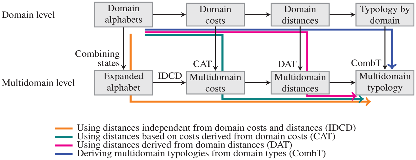
Strategies for building a joint typology.

The first path in the figure has been followed, for example, by Eisenberg-Guyot et al. (2020). With this strategy, the number of costs that must be set may become very large because the number of combinations of domain state tokens increases multiplicatively with the numbers of tokens in each domain. Therefore, some authors (Gauthier et al. 2010; Pollock 2007; Stovel, Savage, and Bearman 1996) prefer to derive MD costs additively from domain costs, which is path 2. Currently, this “cost additive trick” (CAT) is perhaps the most frequently adopted strategy; it is also the only method explicitly implemented in the TraMineR sequence analysis software (Gabadinho et al. 2011); it was used, for example, by Delaporte and Kulu (2023), Möhring and Weiland (2021), and Kang (2022). Regarding the third path, some authors (e.g., Han and Moen 1999) propose that MD distances may be defined by additively combining distances computed separately for each domain. We call this method the “distance additive trick” (DAT). One can also use more elaborate methods based on numerical representations of sequences to derive MD distances from domain distances (e.g., Robette, Bry, and Lelièvre 2015). The fourth strategy—cross-classifying the typologies of the different domains—is not very popular because it produces rapidly too many and often sparse MD types when the number of types per domain increases (Raab and Struffolino 2022:chap. 5).

As we will show, the four approaches can produce very different or even misleading results. Therefore, it is important to understand the assumptions behind a chosen method and the consequences of using it when the assumptions are not satisfied. In particular, we will show that summing domain distances—the DAT strategy—assumes that the trajectories followed in the different domains are independent of each other and that deriving MD costs by adding domain costs—the CAT strategy—assumes state independence across domains.

Analyzing the relationship between domains is of interest only when domains are linked. Therefore, one should evaluate the strength of the association between domains before conducting an MD sequence analysis. The degree of association between domains is useful because it reveals how far we are from the independence condition that CAT and DAT strategies implicitly assume. Because of the importance of the measurement of between-domain association, we briefly address this aspect before discussing the pros and cons of the various strategies with which to build MD typologies.

The main contributions of this article concern the measurement of dissimilarities between MD sequences and the construction of MD typologies. First, with regard to measuring MD dissimilarities, we show that the two most common approaches—computing edit distances with costs additively derived from domain costs, and linear combination of domain distances—implicitly assume independence between domains, and we make explicit the consequences of using such additive procedures when the independence assumption does not hold. We also demonstrate the applicability of the first strategy (IDCD, orange path in Figure 1) with data-driven costs for a large number of combined states by means of an application on real data with three interlocked domains. Second, regarding the combination of domain types, we propose an algorithm to optimally reduce the number of combined types and thereby improve their substantive interpretation. Finally, by applying the various methods to biographic data from the Swiss Household Panel (SHP), we underscore the high sensitivity of the results to the strategy chosen to build the typology. In addition to these key aspects, we introduce the distinction of between-state association between domains from between-trajectory association between domains, which, among other things, proves useful for understanding the difference between the independence assumptions behind the two additive tricks—that is, summing costs (CAT) and summing distances (DAT). We also introduce rules to enhance the visualization by groups/types and domains and help with interpreting typologies of MD sequences.

All calculations in the article were performed within the R platform using the packages TraMineR (Gabadinho et al. 2011) to compute dissimilarities and plot sequences, WeightedCluster (Studer 2013) for clustering, clv (Nieweglowski 2020) for the Rand index, and a user-written seqdomassoc package (available from the first author) for other specific operations, such as domain associations and the optimal merging of joint MD types.

Terminology Used and an Illustrative Toy Example

We consider sequences in which the elements are states assumed by the units of analysis during successive time intervals: for example, employment states experienced by individuals. Each position in a sequence refers to a time interval, such as a year or a month in life-course analysis, or an hour in time-use studies. The set of possible states or tokens forms the alphabet. For clarity, we use the terms token to denote an item in the alphabet and state to refer to an element of the sequence. For instance, a person’s marriage sequence over 20 years from age 20 can be represented by a sequence consisting of five years of singlehood or five “s” (i.e., sssss), five years of cohabitation or five “h,” and 20 years of marriage or 20 “m.” This sequence comprises three state tokens, s, h, and m; the three tokens together form the alphabet for the sequence. Another domain could be parenthood, with, for example, the alphabet of tokens n for no child, and c for having one or more children.

Dissimilarity measures are used to quantify differences between two sequences. We use the terms dissimilarity and distance interchangeably, even though the latter generally refers to measures of differences in Cartesian spaces.

We use OM distances in the data examples we provide in the article. OM measures the dissimilarity between two sequences as the minimal cost for transforming one sequence into the other by means of substitutions, insertions, and deletions of states. OM distances depend on the costs of the basic substitution and indel (insertion or deletion) operations. We opted for data-driven costs, which are user-independent, unlike, for example, theory-based costs. More specifically, we use INDELSLOG (frequency-based method for estimating indel and substitution costs) costs (the term used in the R package TraMineR for a method introduced by Studer and Ritschard 2016:492). INDELSLOG costs are based on the frequency of tokens in the sequences. First, indel costs are set as the logarithm of the inverse of the relative frequency of the tokens—more precisely as log[2/(1 +f)], where f is the relative frequency of the token, to avoid issues with zero frequency—and then the substitution costs between two tokens are derived by summing their indel costs. With such costs, inserting or deleting rare tokens is more costly than inserting or deleting frequent tokens; and substituting rarely observed tokens costs more than substituting common tokens. In addition, INDELSLOG costs are not prone to the limitations of data-driven costs based on transition rates, that is, TRATE (transition rate–based method for estimating substitution costs) costs (Studer and Ritschard 2016:491).

The term multidomain that we use here is equivalent to the term multichannel or multidimensional sometimes used in the sequence analysis literature (e.g., Gauthier et al. 2010; Robette et al. 2015). The alphabet of MD sequences, that is, the set of possible combined domain tokens, is called the “expanded alphabet.” For example, married with children, m+c, is a token of the expanded alphabet of the two domains marriage and parenthood.

To illustrate the issues addressed, we consider the five MD sequences shown in Figure 2 as an example, and we code parenthood state tokens as c for parent and n for no-child, marital status tokens as s for single and m for married, and work tokens as u for no-work and w for work. In this example, the expanded alphabet contains only seven out of the 2³ = 8 possible token combinations because one combination (c+s+u, i.e., parent/single/no-work) does not occur among the five sequences considered.

Figure 2.

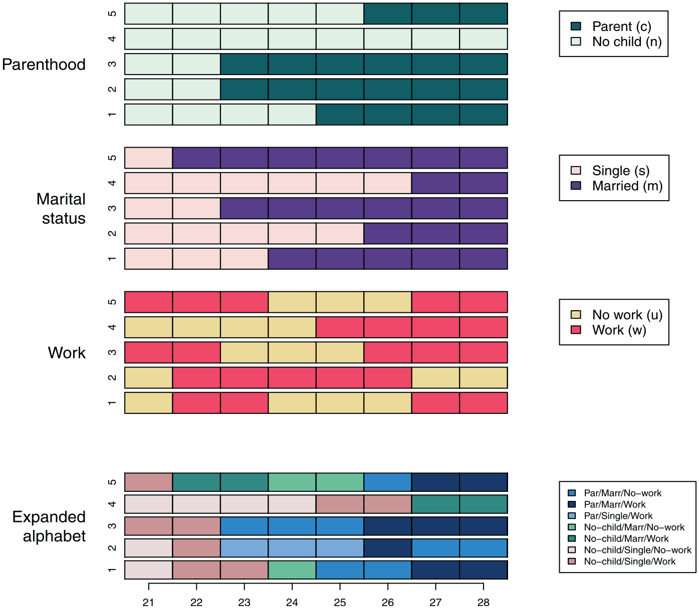
Five multidomain toy sequences over three domains: parenthood, marital status, and work.

Strength of Association between Domains

The hypothetical example in Figure 2 illustrates individual life experiences observed as a series of trajectories unfolding over time in different domains. Clearly, the two domains parenthood and marital status are associated, even though some individuals become a parent without getting married.

The association between domains can be measured and tested at different levels and in different manners. In particular, we introduce the distinction between the association between states and the association between sequences or trajectories. For example, letting living arrangement be a domain with the alphabet {a: alone; b: with both parents; p: with partner; o: with friends} and work be a domain with alphabet {f: full-time work; ℓ: long part-time; s: short part-time; u: unemployed}, consider the two four-time-interval-long MD sequences

\begin{matrix} 1 . (a + f, b + u, p + f, o + u) \\ 2 . (p + f, o + u, a + f, b + u), \end{matrix}

where the notation a+f, for instance, denotes the combination of tokens a of the first domain and f of the second domain, that is, living alone and working full-time. Here we observe state association because full-time, f, in the second domain only occurs with either alone, a, or with partner, p, in the first domain, and unemployed, u, only occurs when living with both parents, b, or with friends, o, and the trajectories, which exhibit a different order in the first domain and are identical in the second domain, do not appear to be associated. Inversely, considering the two MD sequences

\begin{matrix} 3 . (a + ℓ, b + s, p + f, o + u) \\ 4 . (a + u, b + ℓ, p + s, o + f), \end{matrix}

we observe an association between domain trajectories because the relatively long subsequence (ℓ, s, f) of the second domain occurs in both MD sequences together with the same sequence (a, b, p, o) in the first domain. However, there is no state association because the same states of the second domain do not occur at the same positions in the two sequences.

Association between States

The association between the states in two domains measures the tendency of a token in the first domain to co-occur with a token in the second domain. This association can be evaluated by cross-tabulating the states observed in the two domains and computing a categorical association measure, such as Cramer’s v. Here, we can envisage two approaches: (1) cross-tabulating the states of the two domains and (2) cross-tabulating the states of the two domains for each MD sequence, followed by averaging the measured associations over all MD sequences. The second approach, which Piccarreta and Elzinga (2013) considered, is of interest when sequence lengths differ across individuals, because it avoids overweighting individuals with longer sequences.

Table 1 shows the three contingency tables obtained by cross-tabulating two by two the three domains of the example in Figure 2. The three pairs of domains considered are parenthood × marital status, parenthood × work, and marital status × work. The association is quite strong between parenthood and marital status with a Cramer’s v of 0.51 (p = .001). Between parenthood and work, Cramer’s v is as low as 0.0076 and is not statistically significant (p = .96). Likewise, the association between marital status and work is not significant (v = 0.13, p = .43).

Table 1.

Toy Multidomain Sequences; Contingency Tables of State Occurrences

	s	m		u	w		u	w
c	3	16	c	8	11	s	6	11
v = .51**			v = .0076			v = .13
n	14	7	n	9	12	m	11	12

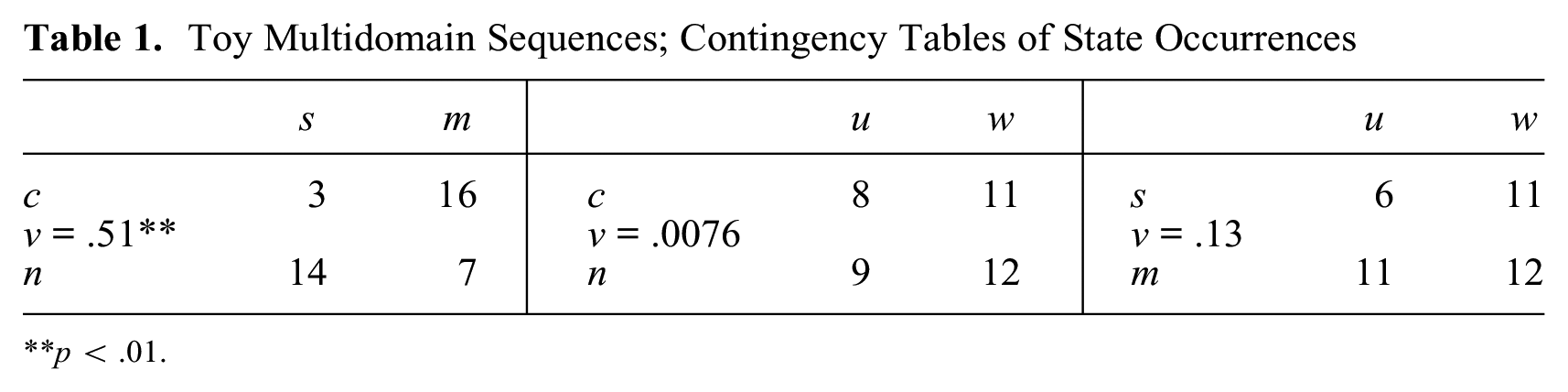
p < .01.

Association between Sequences

The association between sequences in two domains measures how the characteristics of a sequence in the first domain (e.g., states visited, timing, duration, and sequencing) is related to the same characteristics of the sequence in the other domain for the same unit of analysis. Piccarreta (2017) proposed one strategy to quantify the domains’ association: that is, to use Pearson’s or Spearman’s correlation between sequence dissimilarities computed independently for each domain. The dissimilarity between sequences reflects differences in timing, duration, and sequencing of the states. Hence, the correlation between dissimilarities also takes these timing, duration, and sequencing aspects into account. Depending on the metric chosen to measure dissimilarity, each aspect can assume more (or less) importance (Studer and Ritschard 2016).

For the five individuals whose trajectories are displayed in Figure 2, there are 5(5 − 1)/2 = 10 pairwise dissimilarity values for each domain. The association between two domains, parenthood and marital status, for example, is obtained by computing the correlation between the 10 values of these two domains.

Table 2 shows Pearson’s and Spearman’s correlations between pairwise OM distances computed for each domain with INDELSLOG costs. For this and the following analytic steps, we obtain similar results with TRATE-based OM distances, that is, OM distances with costs based on observed transition frequencies (results not shown, available from the authors).

Table 2.

Toy Multidomain Sequences; Association between Domains; State Association (Cramer’s v) and Trajectory Association (Pearson’s r and Spearman’s ρ Correlation between Pairwise INDELSLOG-Based Optimal Matching Distances in Each Domain)

	Cramer’s v	p(v)	Pearson’s r	p(r)	Spearman’s ρ	p(ρ)
Parent with married	.51	.00	.08	.83	.13	.72
Parent with work	.01	.96	.05	.88	.02	.95
Married with work	.13	.43	.35	.32	.37	.30

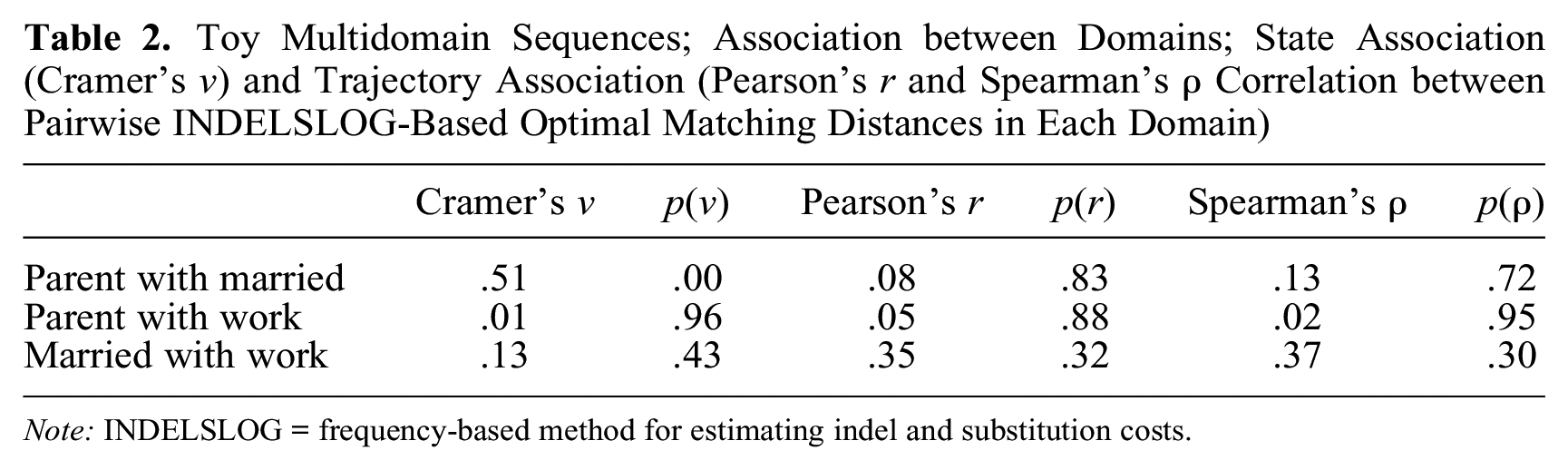
Note: INDELSLOG = frequency-based method for estimating indel and substitution costs.

The highest trajectory association is between married and work. Correlations between both other pairs of domains are very low. In particular, the correlation 0.08 between parenthood and marital trajectories contrasts with the quite strong state association (v) between states of those two domains. This illustrates that state association and trajectory association are distinct concepts. With five cases, there are only 10 pairwise distances for each of the three pairs of domains, which explains why none of the Pearson’s and Spearman’s correlations differs significantly from zero.

Dissimilarities between MD Sequences

In Figure 1, three of the four paths to build MD typologies use MD distances. With the first (orange) strategy, MD distances are computed either using a metric that does not use costs or using IDCD costs, that is, costs set directly at the MD level. With the second (green) strategy, MD distances are computed using costs derived from domain costs. In the third (magenta) path, MD distances are derived from distances within the individual domains. This section examines the pros and cons of these three different strategies to determine MD distances.

IDCD Dissimilarities

Once we have expressed the MD sequences in terms of the expanded alphabet, the first strategy (orange path in Figure 1) is straightforward. Distances are computed as in regular sequence analysis of a single domain by using, if applicable, IDCD costs. However, too large an alphabet size may result from the combination of tokens from the different domains. For instance, three domains with 10 tokens each would lead to an extended alphabet of size 10³ = 1,000. In turn, such a large alphabet dramatically increases the number of indel and substitution costs to set for OM-like edit distances. For the three domains with 10 tokens each, there would be 499,500 substitution costs, and determining them would be a particularly onerous task computationally, if not intractable theoretically.

One solution is to merge nonfrequent states, unless nonfrequent states are the substantive focus of the analysis. This method was used to build the “biofam” sequence data set (Müller, Studer, and Ritschard 2007) of the R package TraMineR (Gabadinho et al. 2011), which was created from three domains: parenthood (child, no child), living with parents (yes, no), and marital status (single, married, divorced). The 12 combined tokens were reduced to eight by grouping together all combined tokens with “yes” for living with parents and all combined tokens with “divorced” as marital status. However, it is difficult to automate this solution and apply it to very large expanded alphabets.

Nonetheless, as we demonstrate with the application in the “Interlocked Domains in Swiss Life-Courses” section, setting substitution and indel costs with data-driven methods and computing the distance matrix requires only a few minutes of computation with alphabets comprising more than 200 tokens after elimination of nonobserved combined ones.

An Additive Trick for MD Costs

Because of the issues raised by large expanded-MD alphabets, some authors have proposed the CAT to determine MD costs from individual domain costs (green path in Figure 1) (see Gauthier et al. 2010; Pollock 2007; Stovel et al. 1996). For the indel, these authors consider only the case of a single state independent indel value, and they determine it by means of the same additive trick. This can be extended to vectors of state dependent indels.

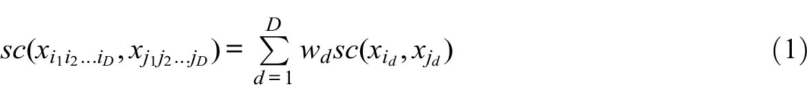
Formally, CAT sets the MD costs as the (weighted) sum of the domain costs of the involved tokens. Let $x_{i_{d}}$ be the ith token of the dth domain, $x_{i_{1} i_{2} \dots i_{D}} = (x_{i_{1}}, x_{i_{2}}, \dots, x_{i_{D}}) \in d_{1} \times d_{2} \dots d_{D}$ , a combined token of the D domains, sc(x_i, x_j) the substitution cost between x_i and x_j, and indel(x_i) the cost of inserting or deleting x_i. The additive substitution and indel costs are

sc (x_{i_{1} i_{2} \dots i_{D}}, x_{j_{1} j_{2} \dots j_{D}}) = \sum_{d = 1}^{D} w_{d} sc (x_{i_{d}}, x_{j_{d}})

(1)

and

indel (x_{i_{1} i_{2} \dots i_{D}}) = \sum_{d = 1}^{D} w_{d} indel (x_{i_{d}}),

(2)

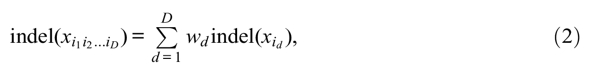
where w_d≥ 0 is the weight attributed to domain d. Such CAT costs verify the triangle inequality when domain costs satisfy the inequality (see Appendix B).

CAT concerns substitution and indel costs and does not apply to distances that do not take into account token dissimilarities, such as the nonaligning distance based on the number of matching subsequences (Elzinga 2003), and the Euclidean and chi-square distances between token distributions.

When substitution costs are set to 1 in all domains and all domain weights w_d equal 1, substitution costs computed by means of CAT correspond to the number of domains on which the combined tokens differ. More generally, when the substitution costs are identical whatever the tokens and domains, the resulting CAT substitution costs are proportional—twice if all substitution costs are 2—to the number of domains on which the two combined tokens differ. This provides a straightforward interpretation. Regarding the indel cost of inserting or deleting a state, in the case of a same unique indel among domains (i.e., the same cost whatever the token and domain), the CAT indel is this unique indel times the number of domains D.

The adequacy of CAT depends on what costs should reflect. For example, if one can justify constant costs for each domain, and if MD costs should reflect the number of domains on which two combined tokens differ, then CAT is the right choice. However, one must ensure that the logic of the strategies for determining costs is consistent between the domain and MD levels. For instance, when using CAT, if one domain is itself MD (e.g., family formation sequences combining parenthood and marital status) and we choose constant costs for it, we must justify a different logic—the CAT logic—for costs when combining that domain with another one (e.g., employment). Likewise, if we opt for INDELSLOG costs at the domain level and want to use the CAT logic for MD costs, a justification for why this state-frequency-based INDELSLOG logic is not adopted at the MD level is necessary.

Independence Assumption behind CAT

CAT has important consequences because it implicitly assumes that states occur independently in each domain. For example, considering the domains parenthood and marital status, CAT sets the same substitution cost between “no child + single” and “child + married” as that between “child + single” and “no-child + married.” In other words, it assumes the state observed at a given position in a given domain is independent from the states occurring at the same position in other domains. This would signify, for instance, that being a parent is independent of marital status. This independence is a strong assumption that has so far been ignored in the literature.

The assumption appears to contradict the objective of MD analysis, which is precisely to study the dependence between domains. However, MD analysis is primarily concerned with the relationships between trajectories in different domains, whereas the independence assumption of CAT concerns states occurrences. As discussed earlier, these are different types of association. The trajectories of two domains may be related even in the case of independence between states of the two domains and, conversely, states of the two domains may be related in the case of independence between domain trajectories.

Nevertheless, whatever the logic used for the domain costs, the CAT cost between the combined tokens $(x_{i_{1}}, x_{i_{2}}, \dots, x_{i_{D}})$ and $(x_{j_{1}}, x_{j_{2}}, \dots, x_{j_{D}})$ will be the same for any pair of combined tokens obtained by exchanging position by position elements between the two original combined tokens, that is, by exchanging i and j indexes at one or more positions d. When the combined tokens differ on all domains, there are $\sum_{d = 1}^{D - 1} (\begin{matrix} D \\ d \end{matrix})$ other pairs that would receive the same CAT substitution cost.

To illustrate the distinctive nature of CAT costs, we compare CAT costs derived from domain-specific INDELSLOG costs (INDELSLOG applied at the domain level) with MD INDELSLOG costs (INDELSLOG applied at the MD level). Consider the five sequences of the domains “parent” and “married” in Figure 2. Table 3 shows the MD INDELSLOG costs and Table 4 the CAT costs.

Table 3.

Toy Multidomain Sequences, Domains Parent and Married; INDELSLOG Costs for Sequences of Combined States

	c+m	c+s	n+m	n+s
c+m	.000	.978	.889	.750
c+s	.978	.000	1.153	1.014
n+m	.889	1.153	.000	.925
n+s	.750	1.014	.925	.000
Indel	.357	.621	.532	.393

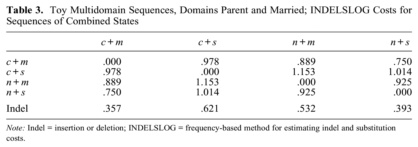
Note: Indel = insertion or deletion; INDELSLOG = frequency-based method for estimating indel and substitution costs.

Table 4.

Toy Multidomain Sequences, Domains Parent and Married; Cost Additive Trick Costs Derived from the Domain-Specific INDELSLOG Costs

	c+m	c+s	n+m	n+s
c+m	.000	.578	.576	1.154
c+s	.578	.000	1.154	.576
n+m	.576	1.154	.000	.578
n+s	1.154	.576	.578	.000
Indel	.543	.643	.510	.610

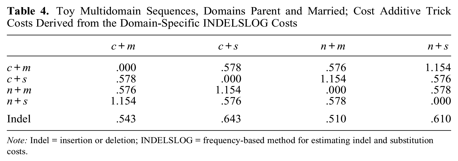
Note: Indel = insertion or deletion; INDELSLOG = frequency-based method for estimating indel and substitution costs.

The symmetry along the second diagonal—sc(c+m, n+s) = sc(c+s, n+m), for example—holds for CAT costs (Table 4) but not for MD INDELSLOG costs (Table 3). Moreover, the CAT substitution costs between combined tokens that differ on both items (on the second diagonal) are about twice the substitution costs between tokens that differ on only one item; this is not true for MD INDELSLOG costs (Table 3). The total number of unique costs in Table 4 is halved when CAT is applied, that is, reduced from six to three. As regards indels, values for frequent combined states (n+s and c+m) are clearly lower than values for less frequent combined states in Table 3 (MD INDELSLOG), whereas CAT indels (Table 4) are much more similar. This example shows that the two approaches may yield very different outcomes. The differences in the results can lead to consequentially different conclusions in empirical research. Therefore, it is important to justify the logic behind setting the costs, and especially CAT costs, in order to justify the assumption of independence between states of different domains.

Appendix C reports results of a simulation analysis of the effects of the independence constraint imposed by CAT. The results of the simulation show that the bias—departure from unconstrained costs—increases with the strength of the state association between domains. More specifically, for the simulated situations, the square root of the computed distortion index—sum of the squared difference between each substitution cost and all the costs that should equal it under the independence assumption—increases linearly with Cramer’s v.

Deriving MD Distances from Domain-Based Distances

A simple method to assess dissimilarities between MD sequences from distances within domains (magenta path in Figure 1) is the DAT (see, e.g., Han and Moen 1999). The DAT consists in summing, or combining linearly, dissimilarities computed separately among the sequences of each domain.

Alternative ways to derive MD distances from domain distances, such as Robette et al. (2015) GIMSA method, are based on principal coordinates of the sequences derived from the dissimilarity matrix in each domain. Unlike additive tricks, such methods do not require any independence assumption, but they are hard to calibrate because of their high sensitivity to the number of principal coordinates retained for each domain. Moreover, GIMSA, for example, applies to the case of two domains only. Instead of principal coordinates of the domains, we could consider numerical indicators of the sequences, such as the mean spell duration, entropy, complexity, turbulence, and, when applicable, integrative capability or insecurity (for details on these indicators, see Ritschard 2021). We do not further detail these approaches here; instead, we focus on DAT.

The DAT strategy assumes that dissimilarity in one domain is independent of the dissimilarity measured in other domains, which implies, for example, that the distance between sequences (c+s, c+s, . . ., c+s), remaining single with children, and (n+m, n+m, . . ., n+m), remaining married without children, is the same as between (n+s, n+s, . . ., n+s), remaining single without children, and (c+m, c+m, . . ., c+m), remaining married with children.

Independence between domain distances can be partially assessed by means of the linear correlation between dissimilarities proposed by Piccarreta (2017). A statistically significant correlation provides evidence for a lack of independence. However, a nonsignificant correlation is not sufficient to support independence, because it does not exclude a nonlinear relationship. To detect nonlinear relationships, one could categorize the distances in each domain into a few classes and test the association between the resulting classes with a nominal association measure, such as Cramer’s v.

An advantage of DAT over CAT is that it works with any distance measure; CAT, in contrast, is limited to edit distances that use indel and substitution costs. Computationally, summing dissimilarities is simple, but it requires first computing and storing dissimilarities for each domain. Computing distance matrices by domain necessitates more memory and computation time than does deriving MD costs with CAT and then computing a single distance matrix with the CAT costs. When the generalized Hamming (i.e., OM without indels) metric is used at the domain and MD levels, the CAT and DAT MD distances are identical (demonstration in Appendix D).

In Table 5 and Figure 3, the sum of domain distances is compared with IDCD (INDELSLOG-based OM distances between MD sequences) and CAT distances for each pair of domains of the toy example. Figure 3 shows the correlation between IDCD, CAT, and DAT distances for the combination of the three domains and each of the three combinations of two domains. In these examples, none of the CAT and DAT distances systematically correlate more strongly with IDCD distances. Surprisingly, the pairwise CAT and DAT distances are identical when we combine the parent and married domains of the toy data. The reason is that here OM distances are equal to the generalized Hamming distances (HAMs) at both the domain and MD levels, that is, the minimal cost for transforming one sequence into the other is achieved for all pairs of sequences with substitutions only. The equality also holds when using TRATE-based costs or a unique substitution cost of 2 with an indel of 1 (results not shown, available from the authors). However, the equivalence with Hamming does not apply for variants of OM, such as OM of spell sequences (Omspell), localized OM (Omloc), OM sensitive to spell length (Omslen), and OM of sequences of transitions (Omstran). For a description of these variants, see Studer and Ritschard (2016).

Table 5.

Pairwise Distances between the Five Toy MD Sequences

	Parent-Married			Parent-Work			Married-Work
	IDCD	CAT	DAT	IDCD	CAT	DAT	IDCD	CAT	DAT
1-2	3.14	2.31	2.31	3.62	3.56	2.68	2.64	2.69	2.69
1-3	1.64	1.73	1.73	1.94	1.73	1.73	.98	1.16	1.16
1-4	3.14	4.04	4.04	4.74	4.34	3.26	3.01	3.77	2.69
1-5	2.74	1.73	1.73	1.92	1.15	1.15	1.87	1.73	1.73
2-3	2.93	1.73	1.73	3.93	3.47	2.03	3.63	3.84	3.77
2-4	5.57	4.03	4.03	5.59	5.39	5.39	3.89	2.99	2.51
2-5	4.38	4.04	4.04	4.65	4.24	3.36	3.65	3.94	3.94
3-4	4.78	5.77	5.77	5.71	5.05	4.51	3.99	4.05	3.37
3-5	3.59	2.30	2.30	2.88	2.20	2.20	1.74	1.53	1.06
4-5	4.10	4.62	4.62	4.78	4.34	3.26	4.88	4.42	4.42

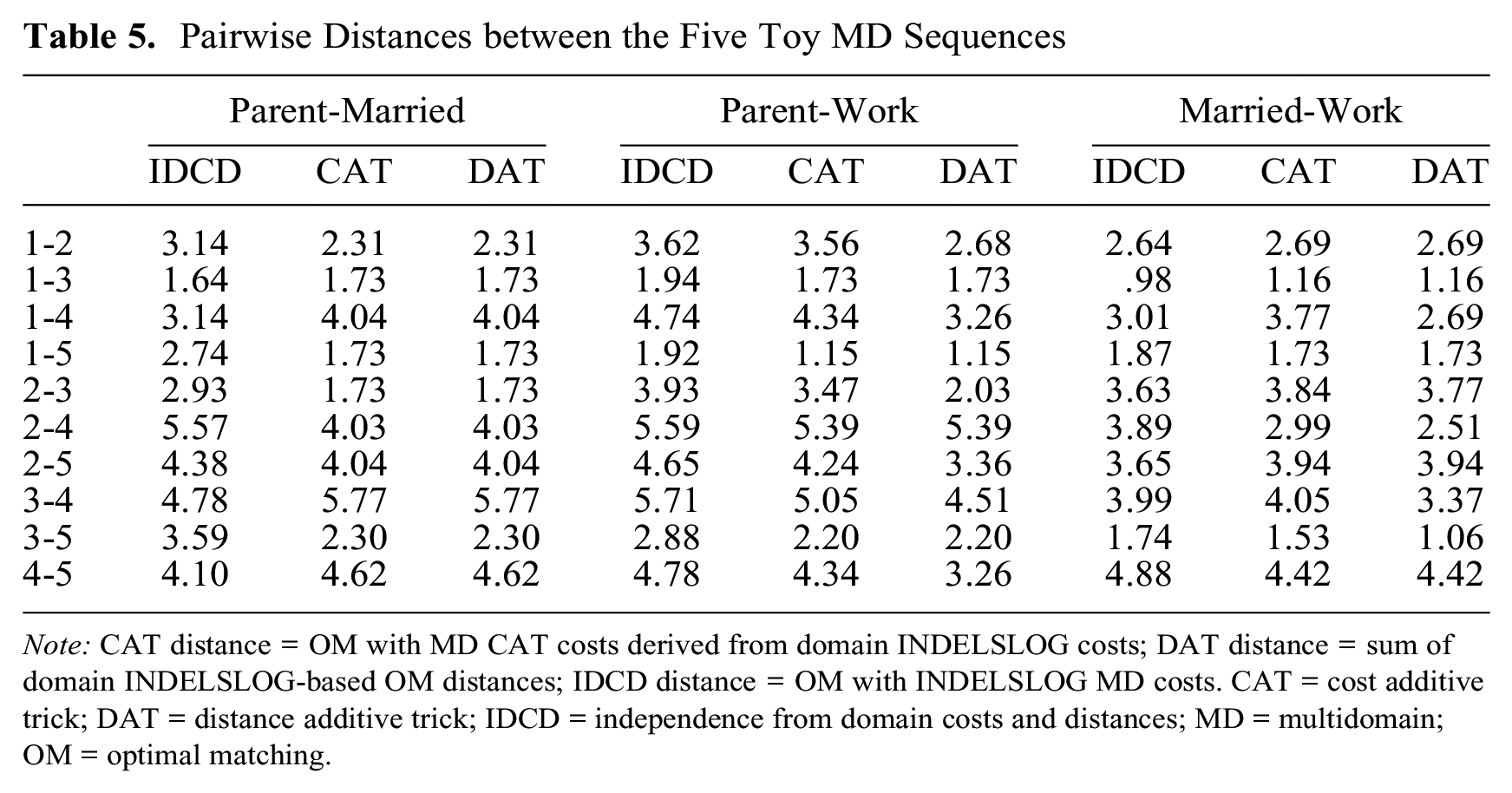
Note: CAT distance = OM with MD CAT costs derived from domain INDELSLOG costs; DAT distance = sum of domain INDELSLOG-based OM distances; IDCD distance = OM with INDELSLOG MD costs. CAT = cost additive trick; DAT = distance additive trick; IDCD = independence from domain costs and distances; MD = multidomain; OM = optimal matching.

Figure 3.

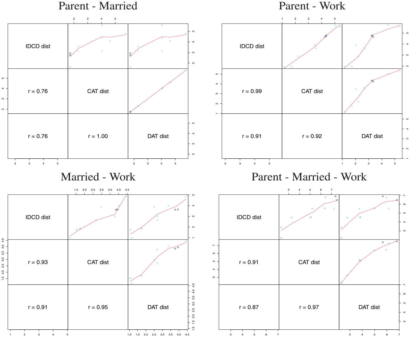
Toy multidomain sequences; correlation between three different measures of multidomain dissimilarities.

Combining Domain Typologies

With the first three strategies (IDCD, CAT, and DAT), the joint MD typology is obtained by clustering the MD sequences from their pairwise MD distances. The difference between these three strategies consists in the method used to compute the MD distances. The fourth strategy (CombT, blue path in Figure 1) bypasses the computation of MD distances and derives the joint typology directly from the typologies built within each separate domain.

The basic principle of this fourth strategy consists in cross-classifying across domains the types identified for each domain. An important issue with such cross-classification is that it results in an unnecessarily large number of groups, including many scarce groups (Raab and Struffolino 2022:chap. 5). Therefore, we recommend supplementing such an operation with an aggregation mechanism that merges poorly represented groups with other groups. For this purpose, we propose an agglomerative method that aims to obtain groups with a user-defined minimum group size, and to minimize the quality loss of the partition.

The proposed algorithm works as follows. If any group is smaller than the wanted minimum group size, first apply the merger that minimizes the quality loss (as judged by a clustering quality criterion) among all possible mergers of the smallest group with another group, and repeat the operation until all group sizes satisfy the size limit. Once no group is smaller than the wanted minimum size, apply the merger that minimizes quality loss among all possible mergers of two groups. Repeat the last operation until the quality loss exceeds a user-defined threshold, which can be set with reference to the quality at the initial partition, at the partition at the previous iteration, or at each iteration to the maximum quality hitherto reached. Alternatively, the process can be stopped when a wanted number of groups is attained.

Any quality measure can be used, such as point biserial correlation, Hubert’s gamma, average silhouette width (ASW), or pseudo R² (for a more complete list, see Studer 2013). Note that pairwise distances between MD sequences are necessary to compute the values of such quality measures, and one should choose among the strategies described in the prior section to compute the distances. The use of MD dissimilarities is necessary to assess the resemblance between the groups to be merged. Ignoring the MD dissimilarities—by choosing, for example, mergers that maximize the agreement of the resulting partition with the initial partition—could lead to the merging of groups with very different profiles.

Visualizing Typologies of MD Sequences

Once an MD typology is identified, the various groups are typically explored using graphics. A first possibility is to render the MD sequences by group using the expanded alphabet, that is, considering the MD sequences as regular sequences. The main problem with this approach is the large size of the extended alphabet, which makes it difficult, if not impossible, to find contrasting colors for the combined tokens and complicates the display of the color legend. The solution we propose is to assign a standard palette of light colors to the entire extended alphabet and then replace the colors of the k most frequent combined tokens—with k being a number between, say, 8 and 12—with a contrasting palette. Restricting the color legend to these k main tokens is often sufficient to identify the salient characteristics of the plots. Moreover, the most frequent combined tokens, together with their frequencies, provide interesting information about the links between the tokens of the different domains.

For a more detailed analysis of the parallel unfolding of the trajectories in the different domains, plotting the sequences separately for each domain is preferable. Such plotting by domain is straightforward for chronograms (or “state distribution plots”), that is, the display of the successive cross-sectional distributions of the states. When the plot depends on choices that themselves depend on the plotted sequence sample, such as the order of the sequences in index plots (where every trajectory is plotted) (Scherer 2001), the selected representative trajectories in plots of representative sequences (Gabadinho and Ritschard 2013), and the sequence order to build equally spaced groups and identify their medoids in relative frequency plots (where a number of medoid sequences efficiently summarize the sample of sequences) (Fasang and Liao 2014), these choices must be made at the MD level and applied to all domains. For example, in Figure 2, the same case order is used for the sequences expressed with the expanded alphabet and for the sequences in each of the three domains, which makes it possible to match sequences by their position. Thus, in the figure, sequence 5 corresponds to the same individual in all index plots shown.

Considering the MD typology, MD analysis consists in exploring the domain-trajectory patterns within each MD type. This requires plotting sequences by type and by domain, as in Figures 4 to 6, which depict the clustering results of the illustrative three-domain analysis of Swiss life-courses (see the next section). In Figures 4 and 5, the plots are organized by three domains (in rows) and four types (in columns). In Figure 5, the sequences in the index plots are sorted by the first principal coordinate vector of the MD distance matrix. Thus, for example, the top sequences in the three plots for the full-timer group (first column) all correspond to the same cases. The representative-sequence plots in Figure 6 are organized with types in rows and domains in columns. The displayed sequences are the domain sequences corresponding to the representative MD sequences of the type. For example, if the fourth MD sequence is a representative sequence of the full-timers, we display, in the full-timers row, the fourth sequence of each domain. The representative sequences of each type are displayed using the same order for each domain. Likewise, the bar heights, which reflect the number of MD sequences assigned to the representative sequences, are also the same for the domain plots of a same type.

Figure 4.

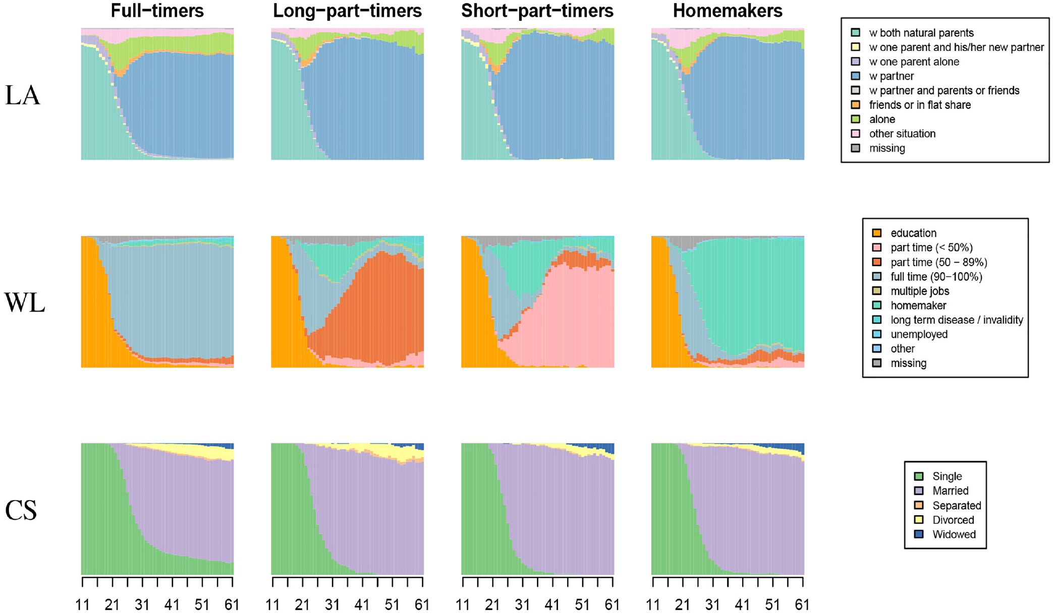
Chronograms of multidomain types (columns) by domain.

Figure 5.

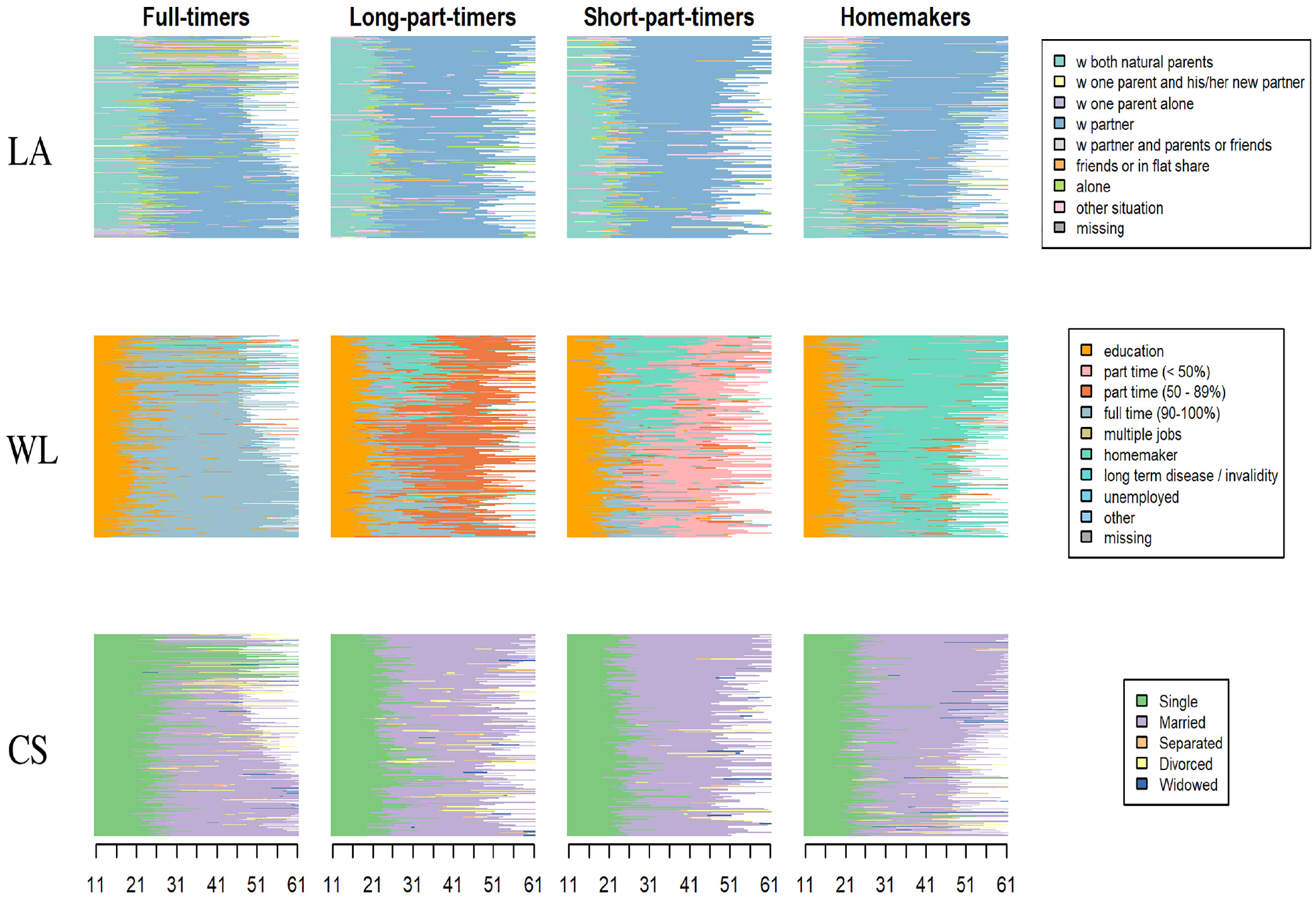
Index plots of multidomain types (columns) by domain.

Figure 6.

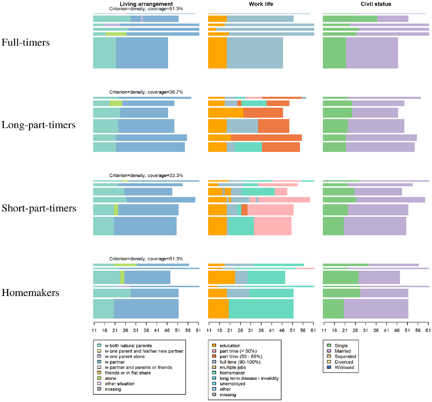
Representative sequences of multidomain types (rows) by domain.

Interlocked Domains in Swiss Life-Courses

To provide an illustrative example, we analyze relationships between different life domains using biographic data from the SHP. This application addresses a core question in life-course research: how do the living arrangement, partnership, and employment trajectories jointly unfold from adolescence to the end of the working life?

Notwithstanding important changes in the course of the past century, Switzerland has been classified as a conservative-liberal welfare state (Esping-Andersen 1990; Scruggs and Allan 2006; Tabin 2002). Several traditionalist elements have continued to characterize the country’s institutional arrangements and social norms: for example, limited childcare options and a traditional gender division of labor have persistently favored a male breadwinner model.

However, Switzerland has experienced trends characterizing the second demographic transition (Lesthaeghe 2010): a more widespread experience of multiple living arrangements after leaving the parental home and before entering a union (typically marriage for the older cohorts, more likely cohabitation for the youngest ones), the postponement of marriage and cohabitation, increased divorce rates, and delayed transition to parenthood.

These demographic dynamics are coupled with transitions out of education into the labor market, which has become more differentiated in recent decades, partly because of the increasing availability of employment arrangements other than full-time jobs (e.g., part-time work) and second jobs (Perrenoud 2020). Temporary contracts and the unemployment rate have remained relatively low compared with most European countries, although long-term unemployment is more widespread than the OECD mean (Lalive and Lehmann 2020). Covering the age span 20 to 45, previous research shows that in Switzerland, employment trajectories have become more destandardized across cohorts in a highly gendered manner (Widmer and Ritschard 2009).

Data

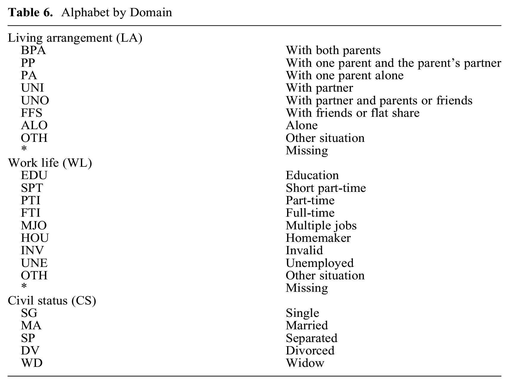
For this illustrative application, we extracted life trajectory sequences from the SHP biographic data collected in 2001 and 2002. We considered three domains: living arrangement (LA), work life (WL), and civil status (CS). For WL, we assume that missing values before the first valid state correspond to education. We reduced—via state merging—the size of the alphabet from 11 to 8 states (plus the missing token) for LA and from 19 to 9 states (plus the missing token) for WL. There are no missing values for CS, and we retained all five valid tokens. Table 6 reports the alphabet for each domain.

Table 6.

Alphabet by Domain

Living arrangement (LA)
BPA	With both parents
PP	With one parent and the parent’s partner
PA	With one parent alone
UNI	With partner
UNO	With partner and parents or friends
FFS	With friends or flat share
ALO	Alone
OTH	Other situation
*	Missing
Work life (WL)
EDU	Education
SPT	Short part-time
PTI	Part-time
FTI	Full-time
MJO	Multiple jobs
HOU	Homemaker
INV	Invalid
UNE	Unemployed
OTH	Other situation
*	Missing
Civil status (CS)
SG	Single
MA	Married
SP	Separated
DV	Divorced
WD	Widow

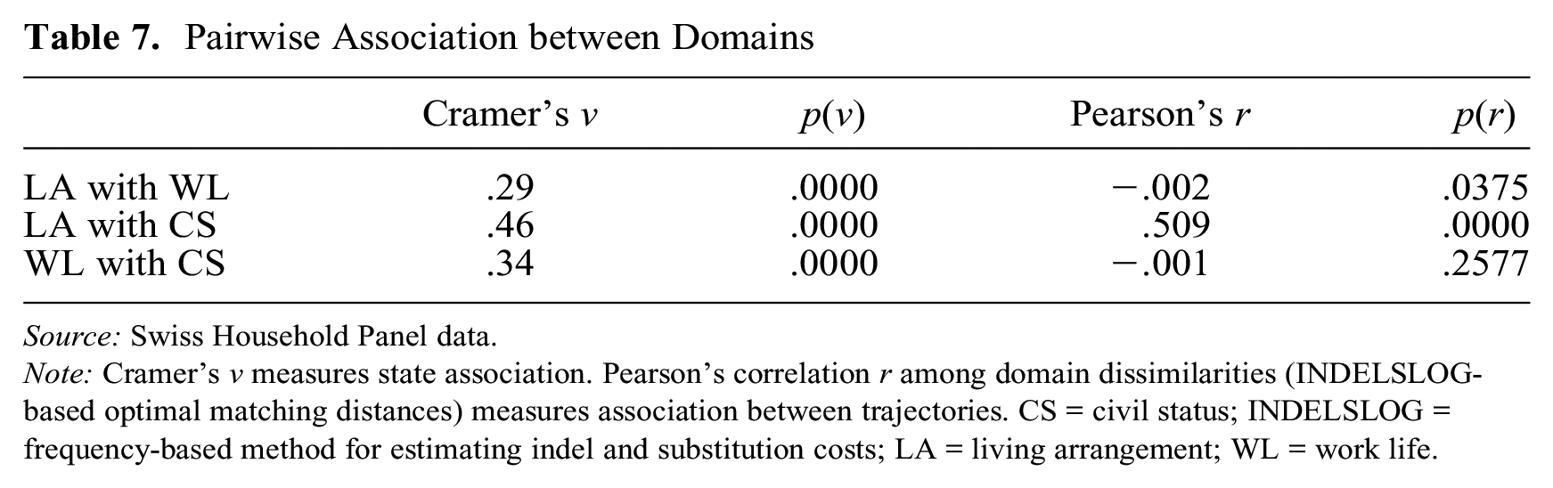
We truncated sequences from the left at age 11 and from the right at age 61 and then dropped sequences with fewer than 36 valid states. The analyzed data comprised 1,903 life sequences between 36 and 51 years’ length of individuals born between 1909 and 1957. This means we had to compute $\frac{n (n - 1)}{2} = 1, 809, 753$ pairwise dissimilarities. The expanded alphabet for the three-domain sequences included 229 observed combined tokens, for which we needed 26,106 substitution costs and 229 indel costs.

Table 7 shows pairwise between-state and between-trajectory association measures for the three domains considered. State association is reflected by Cramer’s v, and trajectory association by Pearson’s correlation r between within-domain dissimilarities. Dissimilarities within each domain are measured with INDELSLOG-based OM distances. We see a clear state association between all three pairs of domains. Regarding trajectory association, the linear correlation between LA and CS is quite strong. The (negative) correlation between LA and WL has poor statistical significance, and the correlation between WL and CS is statistically insignificant. Unsurprisingly, LA and CS are the most tightly linked domains in terms of both state association and trajectory association. These results justify a joint MD analysis. They also provide evidence that using additive tricks, especially CAT, would impose severe restrictions on the resulting MD distances. Therefore, we proceeded with the IDCD strategy, that is, we set costs directly at the MD level.

Table 7.

Pairwise Association between Domains

	Cramer’s v	p(v)	Pearson’s r	p(r)
LA with WL	.29	.0000	−.002	.0375
LA with CS	.46	.0000	.509	.0000
WL with CS	.34	.0000	−.001	.2577

Source: Swiss Household Panel data.

Note: Cramer’s v measures state association. Pearson’s correlation r among domain dissimilarities (INDELSLOG-based optimal matching distances) measures association between trajectories. CS = civil status; INDELSLOG = frequency-based method for estimating indel and substitution costs; LA = living arrangement; WL = work life.

MD Analysis Using IDCD Distances

We now conduct an MD analysis of the three domains LA, WL, and CS, using INDELSLOG-based OM distances between the MD sequences (IDCD distances, orange path in Figure 1). Figures 4 to 6 show chronograms, index plots, and representative sequence plots, respectively, of a partitioning around medoids (PAM) clustering into four groups. In Figure 6, the representative sequences have been searched among the MD sequences using the density criterion with a neighborhood radius of 20 percent of the greatest observed pairwise distance between MD sequences. For each group, the six nonredundant densest MD sequences (i.e., sequences with the densest neighborhood that do not lie in the neighborhood of another densest representative) are displayed separately for each domain. The height of the bars is proportional to the number of sequences assigned to the representative, with each sequence assigned to its closest representative.

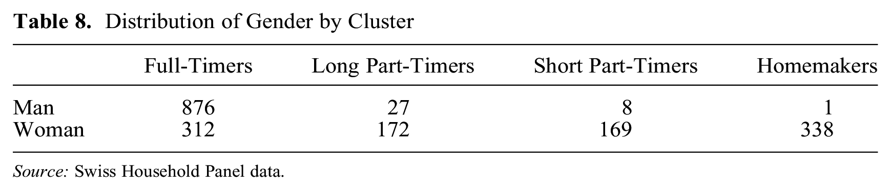
Looking at Figures 4 to 6, it is apparent the clustering is driven by the WL domain. The first group contains trajectories with a long spell of full-time work following education; the second group corresponds to trajectories with an important spell of long part-time employment starting after either education, a full-time job, or a spell at home as a homemaker. The third group comprises people who have short part-time employment after either a period at home, directly after a full-time job, or after a long part-time job. The last group comprises people who stay at home as homemakers after education or after a short period of full-time work. In the Swiss context, where childcare options are limited and social norms as well as the institutional setting have persistently favored the male breadwinner model, women are more likely to experience employment trajectories as identified by the last three clusters. Table 8 confirms that the great majority of men belong to the full-time worker group, whereas women are more equally distributed across the four MD clusters.

Table 8.

Distribution of Gender by Cluster

	Full-Timers	Long Part-Timers	Short Part-Timers	Homemakers
Man	876	27	8	1
Woman	312	172	169	338

Source: Swiss Household Panel data.

There are fewer variations across groups when we consider the other two domains. Nevertheless, we see that living alone is more frequent among full-timers (third group) and almost none of the short part-timers live alone between the ages of 25 and 50; short part-timers are more likely to live with a partner during this age interval. Looking at the CS, full-timers tend to enter marriage later, and the proportion of divorced people is higher among long part-timers and full-timers than in the other two groups.

Clustering Results Based on Alternative Strategies

The foregoing analysis was based on the cluster solution derived from IDCD distances, that is, the first strategy (orange path) in Figure 1. We now examine how the cluster solution would change if we used alternative strategies, namely CAT costs (green path), DAT distances (magenta path), or the merging of combined domain cluster solutions (the CombT solution, blue path). We start with cluster solutions obtained with alternative MD distances.

Figure 7 shows the correlations among IDCD, CAT, and DAT distance measures. CAT and DAT distances are similar (r = .99), but they differ significantly from the IDCD distances used in the previous section. Therefore, we can expect that the typologies obtained using CAT and DAT distances will significantly differ from the typology on the basis of IDCD distances.

Figure 7.

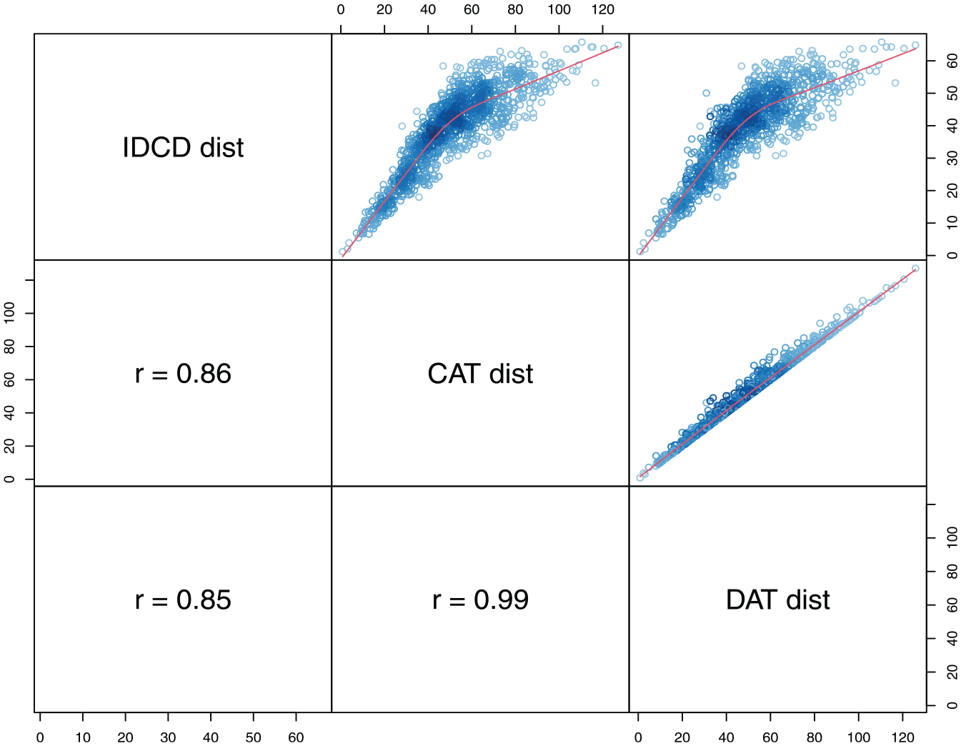
Correlation between different MD measures of dissimilarities between the three-domain sequences.

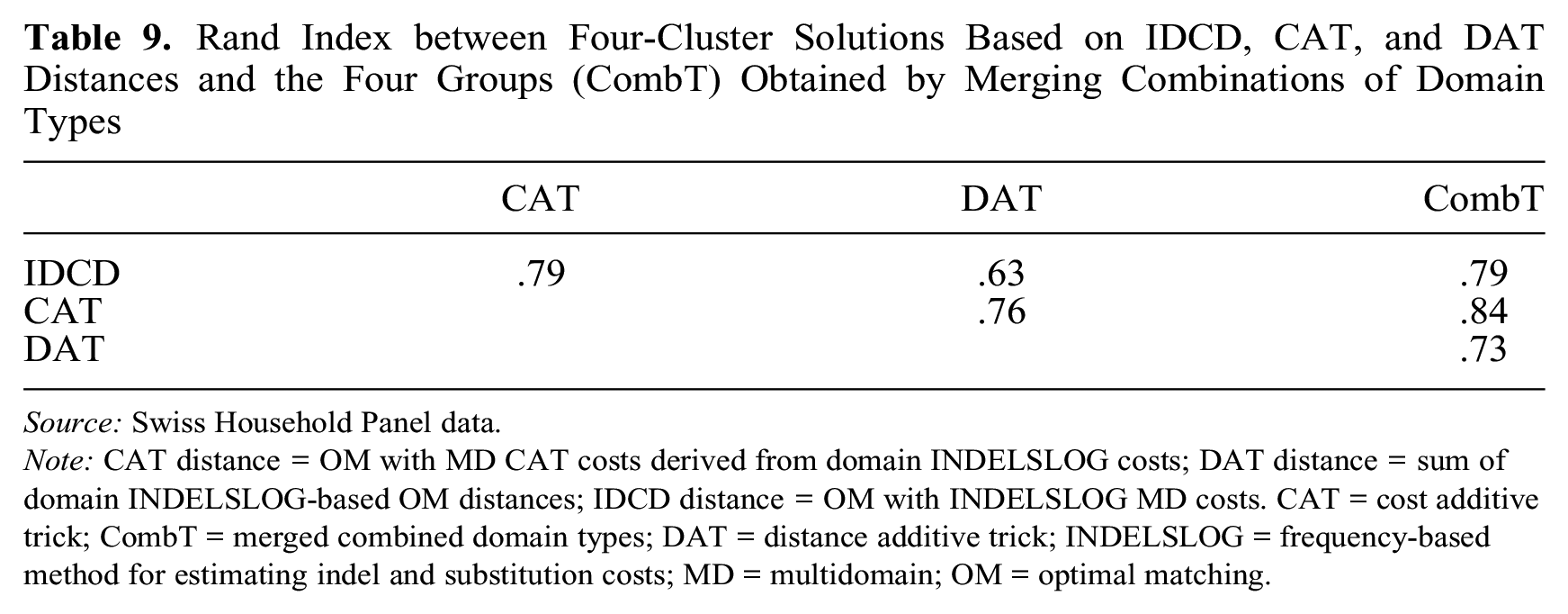
Figure 8 shows chronograms of the three-cluster solutions. Chronograms are displayed using the expanded alphabet of the MD sequences, but the color legend lists only the main (the 12 most frequent) state tokens out of the 229 tokens of the alphabet. The first row in the figure corresponds to the solution based on IDCD distances used in the previous section. The IDCD solution, in which a combined token clearly dominates each type, appears to be the easiest to interpret. The figure shows that the cluster solutions obtained using CAT or DAT distances significantly differ from the IDCD solution. In particular, the content of the third cluster of the CAT and DAT solutions looks very different from the third cluster (short part-timers) of the IDCD solution, and the content of the second cluster of the DAT solution strongly differs from the second cluster (long part-timers) of the IDCD solution. The values of the Rand index in Table 9 confirm that the agreement between IDCD and CAT solutions is closer than between IDCD and DAT solutions.

Figure 8.

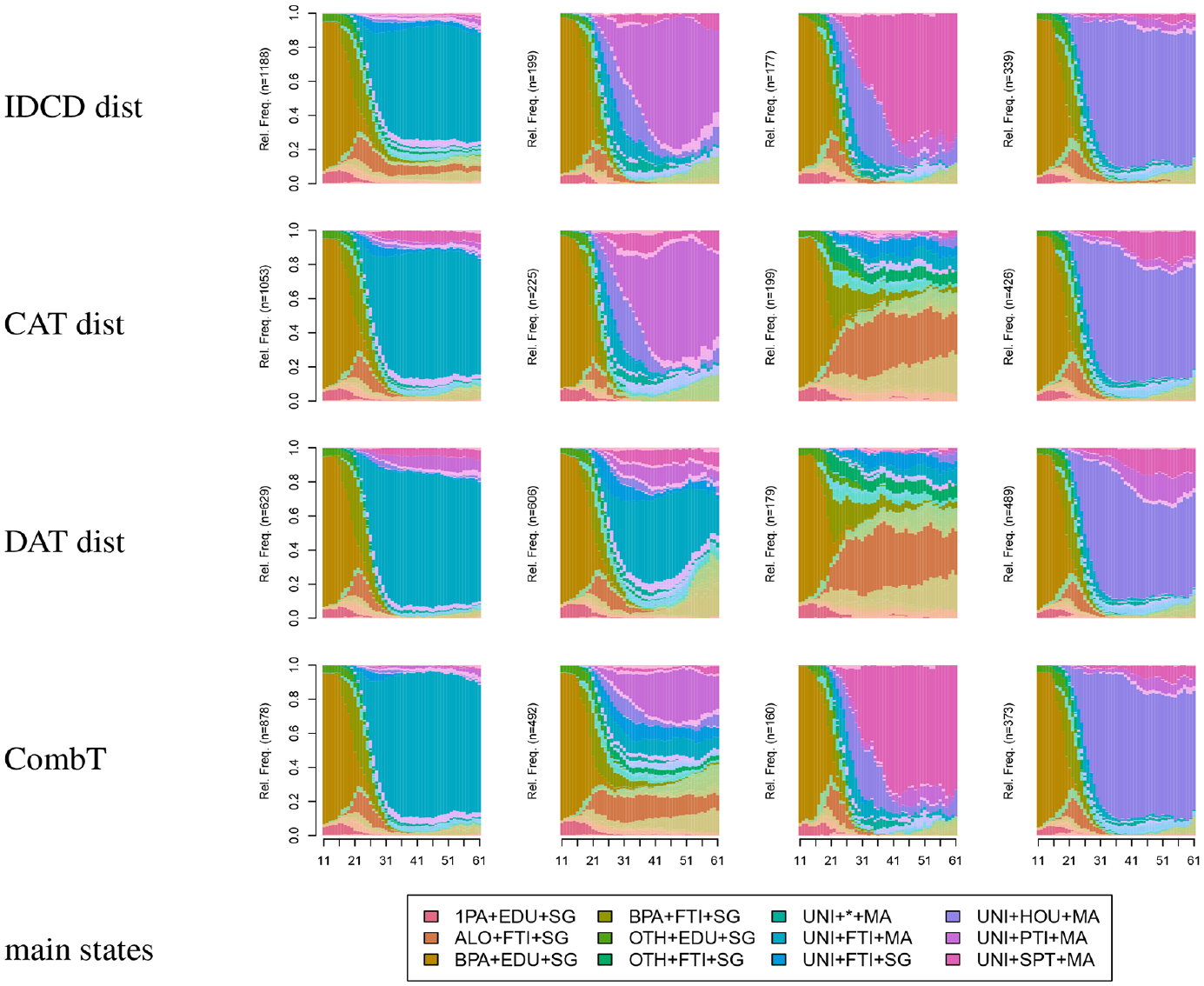
Multidomain sequences combining living arrangement, work life, and civil state domains.

Table 9.

Rand Index between Four-Cluster Solutions Based on IDCD, CAT, and DAT Distances and the Four Groups (CombT) Obtained by Merging Combinations of Domain Types

	CAT	DAT	CombT
IDCD	.79	.63	.79
CAT		.76	.84
DAT			.73

Source: Swiss Household Panel data.

Note: CAT distance = OM with MD CAT costs derived from domain INDELSLOG costs; DAT distance = sum of domain INDELSLOG-based OM distances; IDCD distance = OM with INDELSLOG MD costs. CAT = cost additive trick; CombT = merged combined domain types; DAT = distance additive trick; INDELSLOG = frequency-based method for estimating indel and substitution costs; MD = multidomain; OM = optimal matching.

We now examine the approach on the basis of the ex post combination of the typologies identified by independent clustering of the different domains. From the results displayed in Figures 4 to 6, the MD clustering seems driven mainly by the WL sequences. Therefore, we cluster (using INDELSLOG-based OM distances) the WL domain into four groups, and the two other domains, LA and CS, into two groups. Combining the resulting domain clusters defines a partition into 2 · 4 · 2 = 16 groups. The Rand agreement index with the 16-group cluster solution of the MD sequences is 0.77, indicating that 23 percent of all pairs of sequences that are in the same group of one partition are in different groups of the other partition.

To facilitate comparison with the cluster solutions from the three strategies based on MD distances that we discussed earlier, we reduced the 16 groups of combined domain types to four by successively merging the two groups whose merger maximized the gain in cluster quality—or minimized quality loss in the case of quality deterioration. We selected the ASW as the clustering quality criterion and merged groups until we had four (CombT solution). The last column of Table 9 shows that the agreement with the three solutions based on MD distances ranged from 0.73 (DAT) to 0.84 (CAT). These values indicate that while there is some similarity with the previous solutions, the partition derived from combined domain types markedly differs from the three solutions obtained by clustering MD sequences from their pairwise MD distances. This is confirmed by comparing the last row (CombT) in Figure 8 with the first three rows.

Conclusions

MD sequence analysis examines the relationship between parallel trajectories in several domains. The usual approach consists in building a typology at the MD level and then examining how sequence patterns defined by this joint typology in one domain are related to sequence patterns in other domains. As we have illustrated, the outcomes from this approach are very sensitive to the strategy used to build the MD typology. Like any dissimilarity-based analysis, MD sequence analysis is sensitive to the dissimilarity measure chosen. However, the issue is exacerbated in MD sequence analysis, where one needs dissimilarities at the MD level in addition to dissimilarities measured at the individual domain levels. Such MD dissimilarities can be obtained by applying usual sequence dissimilarity measures to the MD sequences defined with the expanded alphabet (IDCD distances) or by using the tricks proposed in the literature to derive MD dissimilarities from domain characteristics (domain costs for CAT and domain dissimilarities for DAT).

A further approach to building MD typologies is the cross-classification of the types identified at the domain level. A cross-classification of this kind does not require MD dissimilarities. However, it generally generates too many types, so it is frequently unusable. Consequently, we proposed an aggregation process with which to optimally merge cross-classified types. The process uses MD dissimilarities to account for the resemblance between groups, making the outcome also dependent on the strategy chosen to determine MD dissimilarities.

What strategy should be chosen in light of our critical review and assessment? IDCD distances, that is, MD distances computed by considering MD sequences as regular sequences, can be used when their logic makes sense at the MD level. For instance, OM with MD INDELSLOG costs would be justified when one prefers inserting, deleting, and substituting frequently occurring combined tokens to align pairs of MD sequences. The only limitation of edit distances based on substitution and indel costs concerns theory-based costs, which may be difficult, if not impossible, to set and justify when the expanded alphabet becomes very large. Feature-based and data-driven costs remain applicable in any case, and likewise distances that do not use costs such as chi-square distances or distances based on the number of matching subsequences.

The additive tricks (CAT and DAT) furnish simple specific interpretations and can be of interest to sequence researchers. For example, CAT may be justified if one wants to use MD costs to reflect the number of domains on which combined states differ. However, we have shown that CAT assumes state independence among domains and DAT sequence independence among domains. This suggests CAT and DAT should be used only when such assumptions hold, that is, in paradoxical situations of domain independence where it does not make sense to conduct an MD analysis. One may want to use CAT and DAT even if domain independence does not hold, for example, because the resulting costs and distances are simpler to interpret. In such cases, one should be aware of the constraints the procedure imposes between MD costs for CAT and between MD dissimilarities for DAT.

With regard to CAT, analysts should ensure that using MD costs proportional to the number of domain mismatches at the MD level remains coherent with what domain costs reflect. The CAT method applies only to MD distance measures based on substitution and possibly indel costs, whereas the DAT approach, which applies to any distance measure, has a broader scope. To avoid any independence assumptions between domains when computing MD dissimilarities, we suggest using IDCD distances, that is, distances that use neither domain costs nor domain distances. Contrary to what is sometimes stated in the literature, IDCD edit distances remain easily manageable with data-driven costs for large alphabets, as demonstrated in our analysis of three interlocked domains of Swiss life-courses.

Whatever the MD distance used, nothing guarantees the MD cluster solution will be coherent with the groups identified through an independent analysis of each group (for how coherence between MD and domain solutions can be tested, see Piccarreta 2017). Merging combined domain types ensures coherence between MD and domain types by construction. We consequently recommend the combine-and-merge approach when the objective is coherence between MD and domain groups.

Computationally, merging combined domain types is the most time-demanding method because of the merging process. IDCD data-driven costs and CAT costs are computed in a reasonable time span, for example, in less than a minute—using Windows with an I7 processor at 3 GHz with 20 GB random-access memory—for the three domains analyzed in the application. Whatever the costs used, the computation time of pairwise dissimilarities remains the same. Summing distances saves the calculation time necessary to compute MD costs when such costs are required, but it entails the computation of a matrix of pairwise dissimilarities for each domain. Computing such matrices may be necessary in any case if one wants to analyze each domain separately.

In addition to the strategies for building MD typologies, MD analysis requires specific visualization tools with which to present sequences in groups or clusters by domains. In particular, we highlighted that, when plotting individual or representative sequences by groups and domains, one must respect the same sequence order across domains. At present, few computer programs produce plots that can automate such representations. The only one we know of is the R package seqHMM developed by Helske and Helske (2019), which generates an MD index plot. Graphs of this kind warrant further development. Another aspect worth investigating is assessment of the impact of covariates on the association between domains. A potential solution would be to examine the differential correspondence between domain association and covariates. For example, if we observe that the association between family and work trajectories is stronger for women than for men, we will likely have evidence that gender affects domain association.

Footnotes

Appendix A

List of Abbreviations

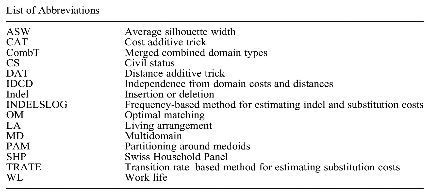
ASW	Average silhouette width
CAT	Cost additive trick
CombT	Merged combined domain types
CS	Civil status
DAT	Distance additive trick
IDCD	Independence from domain costs and distances
Indel	Insertion or deletion
INDELSLOG	Frequency-based method for estimating indel and substitution costs
OM	Optimal matching
LA	Living arrangement
MD	Multidomain
PAM	Partitioning around medoids
SHP	Swiss Household Panel
TRATE	Transition rate–based method for estimating substitution costs
WL	Work life

Appendix B: Triangle Inequality for CAT Costs

If the domain costs applied verify the triangle inequality for each domain, then MD costs derived via CAT satisfy the triangle inequality too.

Appendix C: Simulation: Distortion Induced by CAT

Here, we use a simulation to analyze how the bias introduced by the CAT independence assumption evolves with the strength of the association between domains. We consider three domains with the alphabets {A, B, C}, {G, H, I}, and {X, Y, Z}. At each run, we generate, independently for each domain, n = 1,000 random sequences of length ℓ = 20, with up to four spells in each sequence.

Each sequence is generated by randomly selecting four states (one per spell) in the alphabet and assigning a random number between 1 and ℓ as spell duration. The durations of the last spells are then adjusted such that the total sequence duration is ℓ. For instance, if the selected numbers are 4, 14, 5, and 10, the successive durations will be 4, 14, 2, and 0, and the sequence will contain only three spells. When the sum of the four numbers is less than ℓ, the last duration is expanded to make durations sum to ℓ. For example, drawing 4, 3, 5, and 2, the durations would be 4, 3, 5, and 8.

We then introduce state dependence between the first two domains by randomly selecting for each case a proportion p of the ℓ = 20 positions. At each selected position, where the state of the first domain is the kth element of the alphabet, we turn the state of the second domain also to the kth element of its alphabet. For example, if we have a B (the second element of the first alphabet) at the selected position for the first domain, we force the state at this same position to be an H (the second element of the second alphabet) for the second domain. The larger p, the higher is the tendency of each state of the first domain to co-occur with a specific state of the second domain. We repeat the above run 50 times for each of the five values 0.1, 0.3, 0.5, 0.7, and 0.9 of p.

For each run, we determine substitution costs using the INDELSLOG method. Then, we compute a distortion index to assess by how much costs constrained by the independence assumption depart from unconstrained costs. We define the distortion index as the sum over the pairs of combined state tokens of the squared differences between the substitution cost of the pair and the costs of all pairs that should have the same cost under the independence constraints. The latter are combined tokens obtained by switching between tokens one or two elements of the considered combination. For example, we compare the pair [(A, G, X), (B, G, Y)], with the pairs [(B, G, X), (A, G, Y)], [(A, G, Y), (B, G, X)], and [(B, G, Y), (A, G, X)], that is, with all pairs that would get the same substitution cost as the original pair with CAT. Formally,

(3)

distortion = \sum_{ρ \in P} \sum_{j \in S (ρ)} (s c_{j} - s c_{ρ})^{2},

where P is the set of pairs ρ of combined states, S(ρ) the set of pairs j obtained by switching elements between the pair ρ, and sc_j and sc_ρ the substitution costs for the pairs j and ρ, respectively. Table 10 shows the mean values of the state association between the first two domains as measured by Cramer’s v, the mean value of the distortion, and the standard deviation of the distortion for domain-independence (first row in each panel) and after insertion of dependence between the first two domains (second row in each panel.)

The simulation clearly shows that distortion—sum of squared departure from unconstraint costs—increases with the strength of the state association. Although the distortion is significant in the case of independence, that is, when sequences are generated independently by domain, it remains low and only becomes significantly greater in size with the presence of association. Note, too, that Cramer’s v nicely mimics the proportion of positions in the sequences where we imposed state co-occurrence to generate domain association.

Appendix D: Equality between HAM-Based CAT and DAT Distances

Appendix E: Clusters for Two Two-Domain Analyses

From Table 7, the association between LA and CS is stronger than between LA and WL. We cluster MD sequences, jointly considering successively domains LA and WL, and domains LA and CS. In each case, we compute the PAM four-cluster solution by using IDCD distances (MD INDELSLOG-based OM distances), CAT distances (MD OM distances with CAT costs derived from domain INDELSLOG costs), and DAT distances (sum of domain INDELSLOG-based OM distances.) We evaluate agreement between pairs of cluster solutions using the Rand index (Rand 1971) (see Table 11). The table also reports the Rand index between the solutions found when jointly clustering the three domains.

Agreement of IDCD with CAT and DAT distances is slightly lower for the more strongly associated domains LA and CS than for LA and WL. More importantly, only the left cluster strongly differs between the IDCD solution and the two others in Figure 9 for LA and WL, whereas there are marked differences for clusters in columns 1 and 4 in Figure 10. For the two clusterings of two-domain sequences, agreement between CAT and DAT based solutions is higher than with IDCD solutions; for the clustering of the three-domain sequences, the best agreement is between IDCD and CAT.

ORCID iDs

Gilbert Ritschard

Tim F. Liao

Author Biographies

Gilbert Ritschard is professor emeritus of statistics at the Geneva School of Social Sciences, University of Geneva. His research interests are in methods for life-course analysis and, in particular, sequence analysis and related approaches. He served as president of the Sequence Analysis Association during its first years, from 2018 to 2020. With his team, he developed the widely used TraMineR tool kit for sequence analysis. He has published on sequence analysis in, among others, Sociological Methods and Research, the Journal of Statistical Software, and the Journal of the Royal Statistical Society: Series A.

Tim F. Liao is a professor and chair of sociology and a professor of applied mathematics and statistics at the State University of New York at Stony Brook. He is also affiliated to University of Illinois, Urbana, IL, USA. His research focuses on social demography, primarily life-course studies, and methodology, especially sequence analysis. He serves as president of the Sequence Analysis Association. He is a deputy editor of Demography and an associate editor of Advances in Life Course Research and serves on the American Sociological Review and Sociological Quarterly editorial boards. He is the 2021 recipient of American Sociological Association Methodology’s Paul F. Lazarsfeld Award.

Emanuela Struffolino is an assistant professor of economic sociology at the University of Milan. She was a postdoctoral fellow at the University of Lausanne and at the WZB Berlin Social Science Center. She was then a guest professor at Freie Universität Berlin and at the Humboldt-Universität zu Berlin. Her research interests include social inequality, life-course sociology, and methods for longitudinal data analysis. She has published in, among others, Sociological Methodology, Demography, Research in Social Stratification and Mobility, and Advances in Life Course Research. With Marcel Raab, she published the book Sequence Analysis for SAGE.

References

Abbott

Andrew

Tsay

Angela

. 2000. “Sequence Analysis and Optimal Matching Methods in Sociology, Review and Prospect.” Sociological Methods and Research 29(1):3–33.

Bernardi

Laura

Huinink

Johannes

Settersten

Richard A.

Jr . 2019. “The Life Cube: A Tool for Studying Lives.” Advances in Life Course Research 41:100258. Doi:10.1016/j.alcr.2018.11.004.

Delaporte

Isaure

Kulu

Hill

. 2023. “Interaction between Childbearing and Partnership Trajectories among Immigrants and their Descendants in France: An Application of Multichannel Sequence Analysis.” Population Studies 77(1):55–70.

Eisenberg-Guyot

Jerzy

Peckham

Trevor

Andrea

Sarah B.

Oddo

Vanessa

Seixas

Noah

Hajat

Anjum

. 2020. “Life-Course Trajectories of Employment Quality and Health in the U.S.: A Multichannel Sequence Analysis.” Social Science and Medicine 264:113327.

Elder

Glen H.

Jr. Johnson

Monica K.

Crosnoe

Robert

. 2003. “The Emergence and Development of Life Course Theory.” Pp. 3–19 in Handbook of the Life Course, edited by Mortimer

J. T.

Shanahan

M. J

. Boston: Springer.

Elzinga

Cees H.

2003. “Sequence Similarity: A Non-aligning Technique.” Sociological Methods and Research 31:214–31.

Esping-Andersen

Gøsta

. 1990. The Three Worlds of Welfare Capitalism. Oxford, UK: Polity.

Fasang

Anette E.

Liao

Tim F

. 2014. “Visualizing Sequences in the Social Sciences: Relative Frequency Sequence Plots.” Sociological Methods & Research 43(4):643–76.

Gabadinho

Alexis

Ritschard

Gilbert

. 2013. “Searching for Typical Life Trajectories Applied to Childbirth Histories.” Pp. 287–312 in Gendered Life Courses: Between Individualization and Standardization. A European Approach Applied to Switzerland, edited by Levy

Widmer

E. D

. Vienna, Austria: LIT-Verlag.

10.

Gabadinho

Alexis

Ritschard

Gilbert

Müller

Nicolas S.

Studer

Matthias

. 2011. “Analyzing and Visualizing State Sequences in R with TraMineR.” Journal of Statistical Software 40(4):1–37.

11.

Gauthier

Jacques-Antoine

Widmer

Eric D.

Bucher

Philipp

Notredame

Cédric

. 2010. “Multichannel Sequence Analysis Applied to Social Science Data.” Sociological Methodology 40(1):1–38.

12.

Han

Shin-Kap

Moen

Phyllis

. 1999. “Clocking Out: Temporal Patterning of Retirement.” American Journal of Sociology 105(1):191–236.

13.

Helske

Satu

Helske

Jouni

. 2019. “Mixture Hidden Markov Models for Sequence Data: The seqHMM Package in R.” Journal of Statistical Software 88(3):1–32.

14.

Kang

Ji Y

. 2022. “Trajectories of Labor Market Inequalities and Health among Employees in Korea: Multichannel Sequence Analysis.” Social Indicator Research 160:381–400.

15.

Lalive

Rafael

Lehmann

Tobias

. 2020. “The Labor Market in Switzerland, 2000–2018.” IZA World of Labor 402:1–11.

16.

Lesthaeghe

Ron

. 2010. “The Unfolding Story of the Second Demographic Transition.” Population and Development Review 36(2):211–51.

17.

Liao

Tim F.

2021. “Using Sequence Analysis to Quantify How Strongly Life Courses Are Linked.” Sociological Science 8(3):48–72.

18.

Liefbroer

Aart C.

Elzinga

Cees H

. 2012. “Intergenerational Transmission of Behavioural Patterns: How Similar Are Parents’ and Children’s Demographic Trajectories?” Advances in Life Course Research 17:1–10.

19.

Möhring

Katja

Weiland

Andreas P

. 2021. “Couples’ Life Courses and Women’s Income in Later Life: A Multichannel Sequence Analysis of Linked Lives in Germany.” European Sociological Review 38(3):271–388.

20.

Müller

Nicolas S.

Studer

Matthias

Ritschard

Gilbert

. 2007. “Classification de Parcours de Vie à l’Aide de l’Optimal Matching [Clustering Life-Courses with Optimal Matching].” Pp. 157–60 in XIVe Rencontre de la Société Francophone de Classification (SFC 2007). Paris, France: Société Francophone de Classification.

21.

Nieweglowski

Lukaz

. 2020. “clv: Cluster Validation Techniques.” Reference Manual, Comprehensive R Archive Network. R package version 0.3-2.2. Retrieved March 18, 2023. https://cran.r-project.org/web/packages/clv/index.html.

22.

Perrenoud

Silvia

, ed. 2020. “Quality of Employment in Switzerland 2008–2018.” No. 1227-1800 in Swiss Statistics on Work and Income. Neuchâtel, Switzerland: Federal Statistical Office. Retrieved March 18, 2023. https://dam-api.bfs.admin.ch/hub/api/dam/assets/11607882/master.

23.

Piccarreta

Raffaela

. 2017. “Joint Sequence Analysis: Association and Clustering.” Sociological Methods & Research 46(2):252–87.

24.

Piccarreta

Raffaela

Elzinga

Cees H

. 2013. “Mining for Association between Life Course Domains.” Pp. 190–220 in Contemporary Issues in Exploratory Data Mining in the Behavioral Sciences, edited by McArdle

J. J.

Ritschard

. New York: Routledge.

25.

Pollock

Gary

. 2007. “Holistic Trajectories: A Study of Combined Employment, Housing and Family Careers by Using Multiple-Sequence Analysis.”Journal of the Royal Statistical Society Series A: Statistics in Society 170(1):167–83.

26.

Raab

Marcel

Struffolino

Emanuela

. 2022. Sequence Analysis. Thousand Oaks, CA: Sage.

27.

Rand

William M.

1971. “Objective Criteria for the Evaluation of Clustering Methods.” Journal of the American Statistical Association 66(336):846–50.

28.

Ritschard

Gilbert

. 2021. “Measuring the Nature of Individual Sequences.” Sociological Methods & Research. doi:10.1177/00491241211036156.

29.

Robette

Nicolas

Bry

Xavier

Lelièvre

Eva

. 2015. “A ‘Global Interdependence’ Approach to Multidimensional Sequence Analysis.” Sociological Methodology 45(1):1–44.

30.

Roux

Jonathan

Kingwell

Elaine

Zhu

Feng

Tremlett

Helen

Leray

Emmanuelle

, and the BEAMS Study Group. 2022. “Care Consumption of People with Multiple Sclerosis: A Multichannel Sequence Analysis in a Population-Based Setting in British Columbia, Canada.” Multiple Sclerosis Journal 28(2):309–22.

31.

Scherer

Stefani

. 2001. “Early Career Patterns: A Comparison of Great Britain and West Germany.” European Sociological Review 17(2):119–44.

32.

Scruggs

Lyle

Allan

James

. 2006. “Welfare-State Decommodification in 18 OECD Countries: A Replication and Revision.” Journal of European Social Policy 16(1):55–72.

33.

Stovel

Katherine

Savage

Michael

Bearman

Peter

. 1996. “Ascription into Achievement: Models of Career Systems at Lloyds Bank, 1890–1970.” American Journal of Sociology 102(2):358–99.

34.

Studer

Matthias

. 2013. “WeightedCluster Library Manual: A Practical Guide to Creating Typologies of Trajectories in the Social Sciences with R.” LIVES Working Papers 24. Chavannes-près-Renens, Switzerland: NCCR LIVES.

35.

Studer

Matthias

Ritschard

Gilbert

. 2016. “What Matters in Differences between Life Trajectories: A Comparative Review of Sequence Dissimilarity Measures.” Journal of the Royal Statistical Society Series A: Statistics in Society 179(2):481–511.

36.

Tabin

Jean-Pierre

. 2002. “Les Nouvelles Régulations Politiques de la Question Sociale: Illustrations en Suisse d’un Phénomène Global” [“The New Political Regulations of the Social Question: Swiss Illustrations of a Global Phenomenon”]. Déviance et Société 26(2):221–31.

37.

Widmer

Eric D.

Ritschard

Gilbert

. 2009. “The De-standardization of the Life Course: Are Men and Women Equal?” Advances in Life Course Research 14(1–2):28–39.

Strategies for Multidomain Sequence Analysis in Social Research

Abstract

Keywords

Terminology Used and an Illustrative Toy Example

Strength of Association between Domains

Association between States

Association between Sequences

Dissimilarities between MD Sequences

IDCD Dissimilarities

An Additive Trick for MD Costs

Independence Assumption behind CAT

Deriving MD Distances from Domain-Based Distances

Combining Domain Typologies

Visualizing Typologies of MD Sequences

Interlocked Domains in Swiss Life-Courses

Data

MD Analysis Using IDCD Distances

Clustering Results Based on Alternative Strategies

Conclusions

Footnotes

Appendix A

Appendix B: Triangle Inequality for CAT Costs

Appendix C: Simulation: Distortion Induced by CAT

Appendix D: Equality between HAM-Based CAT and DAT Distances

Appendix E: Clusters for Two Two-Domain Analyses

ORCID iDs

Author Biographies

References