Sage Journals: Discover world-class research

Abstract

Currently available (classical) testing procedures for the network autocorrelation can only be used for falsifying a precise null hypothesis of no network effect. Classical methods can be neither used for quantifying evidence for the null nor for testing multiple hypotheses simultaneously. This article presents flexible Bayes factor testing procedures that do not have these limitations. We propose Bayes factors based on an empirical and a uniform prior for the network effect, respectively, first. Next, we develop a fractional Bayes factor where a default prior is automatically constructed. Simulation results suggest that the first two Bayes factors show superior performance and are the Bayes factors we recommend. We apply the recommended Bayes factors to three data sets from the literature and compare the results to those coming from classical analyses using p values. R code for efficient computation of the Bayes factors is provided.

Keywords

network autocorrelation model hypothesis testing Bayes factor fractional Bayes factor informative prior

The network autocorrelation model (Ord 1975) has been extensively used to represent theories of social influence throughout recent decades. It allows researchers to quantify the strength of a peer effect in a network for a given theory of interpersonal influence while controlling for sociological and other covariates. The identification and magnitude of the peer, or network, effect ρ, also known as the network autocorrelation, is often the focus of interest in model applications. Typically, a researcher aims to identify whether there is social influence present in the network, resulting in an inferential test of $H_{0} : ρ = 0$ versus $H_{1} : ρ \neq 0$ . Subsequently, if the null hypothesis is rejected, the researcher then concludes that there is evidence for some degree of social influence.

Even though the network autocorrelation model and this statistical approach have yielded many interesting and theoretically useful findings, more intricate hypothesis tests are often more informative. For example, when a researcher is interested in testing whether the degree of social influence is zero, small, medium, or large, a more informative test would be $H_{0} : ρ = 0$ versus $H_{1} : 0 < ρ \leq .25$ versus $H_{2} : .25 < ρ \leq .5$ versus $H_{3} : .5 < ρ < 1$ . This not only allows a researcher to conclude whether there is evidence for a nonzero amount of network autocorrelation in the network, but it grants the researcher the opportunity to simultaneously test several strengths of social influence against each other as well. This article focuses on Bayesian hypothesis testing procedures for such multiple precise and interval hypotheses for the network autocorrelation.

The standard approach to testing a network effect is null hypothesis significance testing. Classical null hypothesis significance tests such as the Wald test, the likelihood ratio test, or the Lagrange multiplier test are based on different test statistics, summary values constructed from the sample, which have asymptotically known distributions under the null hypothesis (Leenders 1995). Then, assuming the null hypothesis to be true, the probability of observing a test statistic at least as extreme as the observed test statistic is calculated. This probability is called the “p value.” Subsequently, the p value is compared to a prespecified significance level α which is usually set to .05 (Weakliem 2004). If the p value is smaller than α, the null hypothesis is rejected. In this case, one would conclude that there is enough evidence in the data to reject the null hypothesis of no network effect. If the p value is larger than α, there is not enough evidence in the data to reject the null.

Classical null hypothesis significance testing in the network autocorrelation model has a number of disadvantages. First, the procedure cannot be used to provide evidence in favor of the null hypothesis (Wetzels and Wagenmakers 2012); it can only falsify the null hypothesis. If the p value is larger than α, this ultimately implies a state of ignorance where the null can be neither rejected nor supported by the data. For example, if the estimated autocorrelation parameter is $\hat{ρ} = .16$ with a two-sided p value of .08 (so the null hypothesis that ρ = 0 would not be rejected based on α = .05), this does not mean that the null hypothesis is “accepted”; it merely means that judgment regarding the rejection of this particular hypothesis is suspended and that no degree of belief in the hypothesis has been determined. On the other hand, if the p value is smaller than α, it is still not possible to say how much evidence there is against the null (and certainly not how much evidence there is in favor of ρ being .16 indeed), only that there is enough evidence to reject the null that ρ = 0 based on a chosen significance level. Second, classical null hypothesis significance tests are not consistent. If the null is true and the sample size grows to infinity, there is still a probability of α (typically .05) of drawing the incorrect conclusion that the null is false. This is undesirable, as one should be able to draw more accurate conclusions with growing sample size. Third, p values in the network autocorrelation model depend heavily on asymptotic theory and consequently, the type I error probability is not controlled for in an accurate manner in the case of small networks (Dittrich, Leenders, and Mulder 2017). A final important issue in the context of this article is that p values cannot be adequately used when testing multiple competing hypotheses against each other (Shaffer 1995). Instead, one can only test each hypothesis against the null which does not answer the question which hypothesis, out of a set of precise and interval hypotheses, is most supported by the data.

In this article, we propose Bayes factor tests (Jeffreys 1961; Kass and Raftery 1995; Mulder and Wagenmakers 2016) as an alternative approach to classical null hypothesis significance testing in the network autocorrelation model. The Bayes factor is a Bayesian hypothesis testing criterion that circumvents the aforementioned issues with null hypothesis significance testing. First, in contrast to classical null hypothesis significance testing, it allows the researcher to evaluate and quantify the relative evidence in the data in favor of the null, or any other, hypothesis against another hypothesis (Kuha 2004). These hypotheses can be precise hypotheses, for example, $H_{0} : ρ = 0$ , or interval hypotheses, for example, $H_{1} : 0 < ρ < 1$ . For instance, a Bayes factor of $B_{01} = 5$ implies that it is five times more likely to observe the data under H₀ than under a specific alternative hypothesis H₁. Second, Bayes factors are consistent, that is, if H₀ is the true model, the Bayes factor B₀₁ tends to infinity as the sample size goes to infinity (Casella et al. 2009). In other words, the larger the sample size, the more do the data support one hypothesis over another. Third, the Bayes factor provides “exact” inference without the need for asymptotic approximations (De Oliveira and Song 2008). Lastly, the Bayes factor can be straightforwardly extended to test more than two hypotheses against each other, for example, $H_{0} : ρ = 0$ versus $H_{1} : - .25 < ρ < 0$ versus $H_{2} : 0 < ρ \leq .25$ versus $H_{3} : .25 < ρ \leq .5$ versus $H_{4} : .5 < ρ < 1$ (Raftery, Madigan, and Hoeting 1997). This feature is of particular relevance in the network autocorrelation model, as in many network studies, researchers do not doubt that social influence occurs but are interested in testing competing theories about its strength. In summary, these advantageous properties explain the increasing usage of Bayes factors in social science research, such as in linear regression models (Braeken, Mulder, and Wood 2015), analysis of variance (Klugkist, Laudy, and Hoijtink 2005), repeated measures (Mulder et al. 2009), or structural equation modeling (Gu et al. 2014).

So far, only two Bayes factors for the network autocorrelation model have been developed in the literature. Hepple (1995) proposed a Bayes factor for testing competing connectivity matrices against each other, while LeSage and Parent (2007) provided Bayes factors for testing different explanatory variables. We have neither found any Bayes factors for the standard one-sided test $H_{0} : ρ = 0$ versus $H_{1} : 0 < ρ < 1$ nor for any multiple hypothesis tests. This is surprising, as the network autocorrelation parameter is at the heart of the model and testing for network effects is of crucial importance for network scientists when testing for and understanding theories of social influence. In sum, the objective of this article is to provide methodology that

makes it possible to test multiple competing hypotheses regarding ρ against each other and to precisely quantify the amount of evidence in favor of any of the hypotheses tested (including H₀),

works for any combination of precise and/or interval hypotheses, and

overcomes the problems with classical null hypothesis significance testing of ρ.

We also provide ready-to-use R code to make the methodology easily applicable for applied researchers.

In order to compute the Bayes factor, the so-called prior distributions, or simply priors, for the unknown model parameters have to be specified under each hypothesis. These priors quantify which values for the parameters are most likely before observing the data. For the testing problems considered in this work, the prior for the network autocorrelation ρ under the alternative(s) is most important. In this article, we develop and explore several Bayes factors for testing the network effect: first, a Bayes factor based on an empirical informative prior which stems from an extensive literature review of empirical applications of the network autocorrelation model; second, a Bayes factor based on a uniform prior that assumes every value of ρ to be equally likely a priori; third, a so-called fractional Bayes factor (O’Hagan 1995) which can be computed without needing to formulate a proper, that is, integrable, prior distribution for ρ based on one’s prior beliefs. Subsequently, we conduct a simulation study to investigate the numerical properties of and differences between the proposed Bayes factors and then use the Bayes factors to reanalyze three data sets from the literature. Finally, we give efficient R code for the computation of the Bayes factors.

The article is organized as follows: In the second section, we discuss the network autocorrelation model in more detail and continue with a short introduction to Bayesian hypothesis testing in the third section. In the fourth section, we motivate several prior choices for the network autocorrelation parameter ρ. We assess the numerical performance of the Bayes factors in a simulation study in the fifth section and highlight their practical use with three examples in the sixth section. The seventh section concludes.

The Network Autocorrelation Model

Most social phenomena are embedded within networks of interdependencies. Building from a standard linear regression model, the network autocorrelation model effectively incorporates such interdependencies between individuals. In the model, the network structure is explicitly used to account for network influence and to estimate the magnitude of this influence. More specifically, the network influence is considered as a model parameter, the so-called network autocorrelation ρ, and operates directly on the outcome variable. Formally, the network autocorrelation model is expressed as

y = ρ W y + X β + ε, ε \sim N (0, σ^{2} I_{g}),

where y is a (g × 1)-vector of values of a dependent variable for the g network actors, X is a (g × k)-matrix of values for the actors on k covariates, β is a (k × 1)-vector of regression coefficients, I_g denotes the (g × g)-identity matrix, and ε is a (g × 1)-vector containing independent and identically normally distributed error terms with zero mean and variance of σ². Furthermore, W is a given (g × g)-connectivity matrix representing social ties in a network, with $W_{i j} (i, j \in {1, ..., g})$ denoting the degree of influence of actor j on actor i.¹ Finally, the network autocorrelation ρ is the key parameter of the model and quantifies the social influence for given y, W, and X. We denote the resulting set of model parameters as $θ : = (ρ, σ^{2}, β)$ . Subsequently, we will repeatedly rely on the model’s likelihood, given by (e.g., Doreian 1980)

f (y | ρ, σ^{2}, β) = | det (A_{ρ}) | {(2 {πσ}^{2})}^{- \frac{g}{2}} exp (- \frac{1}{2 σ^{2}} {(A_{ρ} y - X β)}^{T} (A_{ρ} y - X β)),

where $A_{ρ} : = I_{g} - ρ W$ . To ensure that the model is well-defined, there are restrictions on the region of support for ρ. Typically, this region is chosen as the interval containing ρ = 0 for which A_ρ is nonsingular (Hepple 1995; LeSage and Parent 2007; Smith 2009). In this case, the corresponding admissible interval for ρ is given by $(λ_{g}^{- 1}, λ_{1}^{- 1})$ where $λ_{1} \geq λ_{2} \geq \dots \geq λ_{g}$ are the ordered eigenvalues of W (Hepple 1995). For row-standardized connectivity matrices W, that is, where each row sum is one, it holds that λ₁ = 1 (Anselin 1982). Without loss of generality, we restrict ourselves to such commonly used row-standardized connectivity matrices in the remainder. Hence, the model’s parameter space becomes $Θ : = Θ_{ρ} \times Θ_{σ^{2}} \times Θ_{β} = (λ_{g}^{- 1}, 1) \times (0, \infty) \times ℝ^{k} .$

Throughout the literature, the model has also been named as mixed regressive–autoregressive model (Ord 1975), spatial effects model (Doreian 1980), network effects model (Marsden and Friedkin 1993), or spatial lag model (Anselin 2002), and it has been applied in many different fields such as sociology (Duke 1993; Kirk and Papachristos 2011; Mizruchi, Stearns, and Marquis 2006), political science (Beck, Gleditsch, and Beardsley 2006; Gimpel and Schuknecht 2003), criminology (Baller et al. 2001; Tita and Radil 2011), or geography (McMillen 2010; Mur, López, and Angulo 2008).

Bayesian Hypothesis Testing

In many network studies, researchers have expectations about the magnitude of the network effect. An interesting research question is whether the network effect can be classified as zero, small, medium, or large. These expectations can be translated to a set of multiple hypotheses on the network autocorrelation by setting H₀ : ρ = 0, H₁ : 0 < ρ ≤ .25, H₂ : .25 < ρ ≤ .5, and H₃ : .5 < ρ < 1, and the question to be answered is which of these hypotheses is most plausible. In general, such a test is much more insightful than the standard test of no network effect versus “some” (positive) network effect, H₀ : ρ = 0 versus H₁ : 0 < ρ < 1. In order to illustrate this, consider a situation in which the estimated network autocorrelation parameter is $\hat{ρ} = .16$ , with a 95 percent confidence interval for ρ of (−.06; 37), and a one-sided p value of .08. Using the standard significance level of α = .05, we would not reject the null hypothesis that ρ = 0 and would conclude that there is no statistically significant network effect present in the data. Based on the confidence interval, however, we do have quite a lot of confidence that the network effect may be positive. Hence, based on these classical outcomes, it is very difficult to state how plausible it is that the true network effect is zero, small, medium, or large, which was the initial research question of the network scientist.

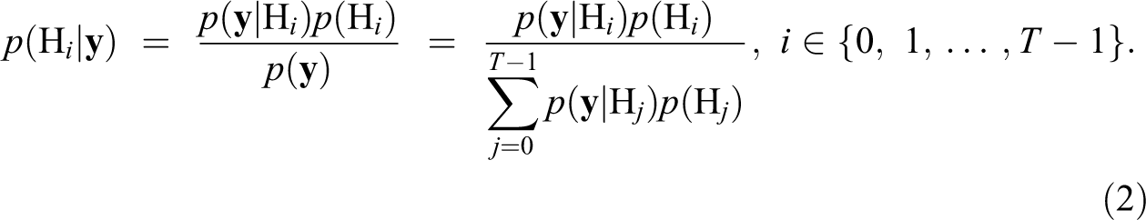
The Bayes factor is a Bayesian hypothesis testing criterion that resolves this issue by providing a means to directly quantify how plausible each hypothesis is after observing the data. Suppose that we are interested in testing T ≥ 2 hypotheses, H₀, H₁, H₂, …, H_T−1. First, in Bayesian hypothesis testing, prior probabilities have to be assigned to both the model parameters under each hypothesis and to the hypotheses themselves. We denote these latter prior hypotheses probabilities by p(H₀), p(H₁),… p(H_T−1), with $\sum_{i = 0}^{T - 1} p (H_{i}) = 1$ , which reflect how plausible we believe each hypothesis to be (relative to each other) before observing the data. There are multiple ways to assign prior hypotheses probabilities, for example, by assuming equal prior probabilities (reflecting prior ignorance), that is, $p (H_{0}) = \dots = p (H_{T - 1}) = 1 / T$ (Hepple 1995; LeSage and Parent 2007), or by formulating specific prior probabilities for the various hypotheses. We will discuss procedures for eliciting prior probabilities of interval hypotheses in the fourth section.

Next, after observing the data y, Bayes’s theorem is applied to update the prior expectations with the information contained in the data. The resulting posterior probabilities of the hypotheses, $p (H_{i} | y)$ , can then be written as:

p (H_{i} | y) = \frac{p (y | H_{i}) p (H_{i})}{p (y)} = \frac{p (y | H_{i}) p (H_{i})}{\sum_{j = 0}^{T - 1} p (y | H_{j}) p (H_{j})}, i \in {0, 1, \dots, T - 1} .

These posterior probabilities quantify how probable each hypothesis is after observing the data, thus the quantity that researchers are typically interested in. The higher the posterior probability of a particular hypothesis, the stronger the evidence in the data in favor of that hypothesis.

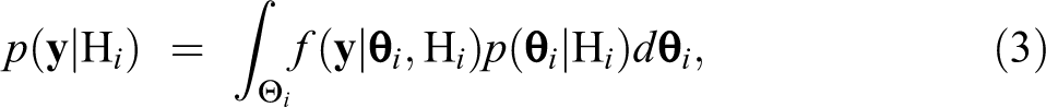
The term $p (y | H_{i})$ in equation (3) is called the marginal likelihood of the data y under the hypothesis H _i and denotes the probability that the data were observed under this specific hypothesis H _i . It is computed by integrating the product of the model’s likelihood function and the prior distribution for the model parameters under H _i . Hence, the marginal likelihood can be seen as a weighted likelihood over the parameter space under H _i , with the prior under H _i acting as a weight function. In formal notation,

p (y | H_{i}) = \int_{Θ_{i}} f (y | θ_{i}, H_{i}) p (θ_{i} | H_{i}) d θ_{i},

where θ_i are the model parameters under H_i, $p (θ_{i} | H_{i})$ their prior density, and Θ_i the corresponding parameter space. For instance, for $H_{0} : ρ = 0$ and $H_{1} : 0 < ρ < 1$ in the network autocorrelation model (1), it follows that $θ_{0} = (σ^{2}, β)$ , $Θ_{0} = ℝ^{+} \times ℝ^{k}$ , and $θ_{1} = (ρ, σ^{2}, β)$ , $Θ_{1} = (0, 1) \times ℝ^{+} \times ℝ^{k}$ .

When performing pairwise model comparisons between two hypotheses H _i and H _j , we can consider the ratio of the corresponding two posterior probabilities of the hypotheses. In this case, the normalizing constant p(y) in equation (3) cancels out, and we can write

\frac{p (H_{i} | y)}{p (H_{j} | y)} = \frac{p (y | H_{i})}{p (y | H_{j})} \times \frac{p (H_{i})}{p (H_{j})} : = {BF}_{i j} \times \frac{p (H_{i})}{p (H_{j})} .

The term $p (H_{i}) / p (H_{j})$ in equation (5) is called the prior odds of the two hypotheses and quantifies how much more, or less, likely the researcher expected H _i to be compared to H _j before observing the data y. When a researcher does not a priori believe one being more likely than the other, the prior odds can be set equal to one. The term on the left-hand side of equation (5), $p (H_{i} | y) / p (H_{j} | y)$ , is known as the posterior odds, reflecting how much more (if larger than one) or less (if smaller than one) likely H _i is than H _j after taking the observed data into account. For example, if the posterior odds are five, this means that H _i is five times more likely than H _j for this data set. From equation (4), we can see that the posterior odds can be written as the prior odds multiplied by the Bayes factor, BF_ij, which is defined as the ratio of the marginal likelihoods. Hence, the Bayes factor indicates to which extent the data change the prior odds to the posterior odds. Note that the Bayes factor can be used for quantifying the relative evidence between hypotheses without needing to specify how plausible the hypotheses are before observing the data. If both models are considered as equally likely a priori, that is, $p (H_{i}) = p (H_{j})$ , the Bayes factor equals the posterior odds.

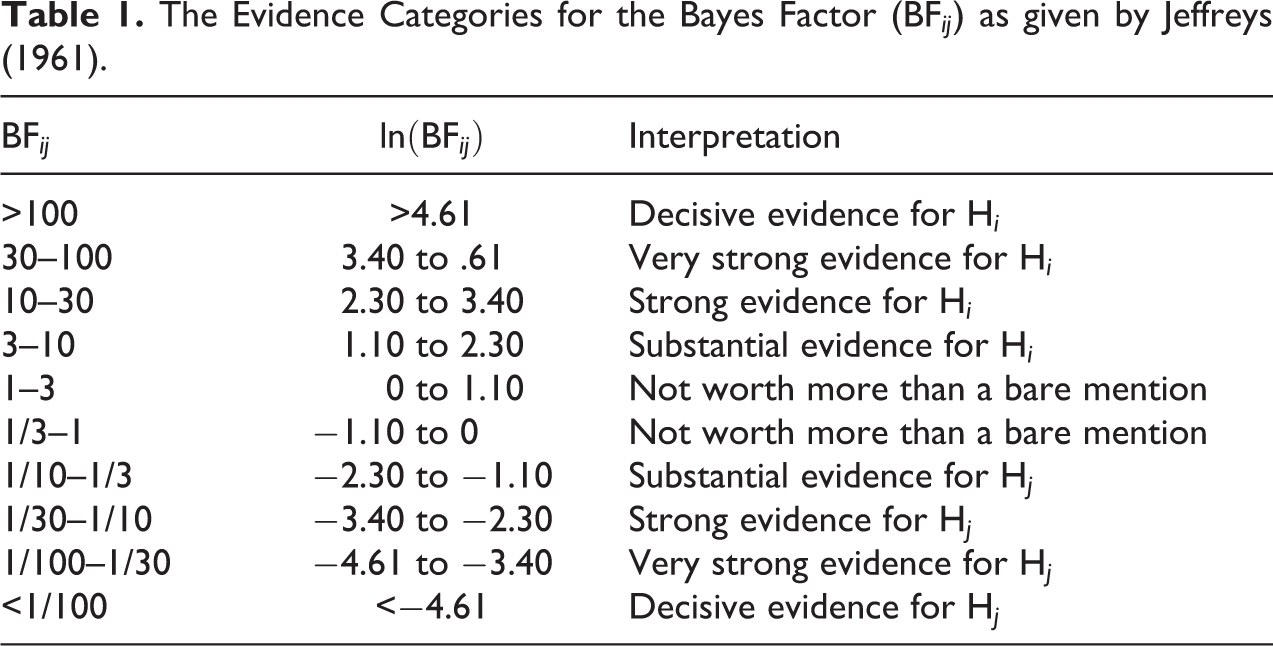
The Bayes factor is a measure of relative evidence; it quantifies the amount of evidence in the data in favor of one hypothesis relative to another hypothesis. Jeffreys (1961) proposed a classification scheme to group Bayes factors into different categories (see Table 1). For example, there is “substantial” evidence for H _i when the Bayes factor exceeds 3 and, equivalently, substantial evidence for H _j when the Bayes factor is less than 1/3. These labels provide some rough guidelines when speaking of relative evidence in favor of a hypothesis, but the interpretation should ultimately depend on the context of the research question (Kass and Raftery 1995).

Table 1.

The Evidence Categories for the Bayes Factor (BF_ij) as given by Jeffreys (1961).

BF_ij	$ln ({BF}_{i j})$	Interpretation
>100	>4.61	Decisive evidence for H_i
30–100	3.40 to .61	Very strong evidence for H_i
10–30	2.30 to 3.40	Strong evidence for H_i
3–10	1.10 to 2.30	Substantial evidence for H_i
1–3	0 to 1.10	Not worth more than a bare mention
1/3–1	−1.10 to 0	Not worth more than a bare mention
1/10–1/3	−2.30 to −1.10	Substantial evidence for H_j
1/30–1/10	−3.40 to −2.30	Strong evidence for H_j
1/100–1/30	−4.61 to −3.40	Very strong evidence for H_j
<1/100	<−4.61	Decisive evidence for H_j

Bayes Factor Tests for the Network Autocorrelation Parameter

In this section, we propose three Bayes factor tests when considering precise hypotheses, $H_{precise} : ρ = c$ , and interval hypotheses, $H_{interval} : a_{1} < ρ < a_{2}$ , for the network autocorrelation parameter. One of the most important steps in Bayesian hypothesis testing is the prior specification of the model parameters. In the network autocorrelation model (equation 1), a prior for ρ must be specified under an interval hypothesis, while no prior for ρ needs to be formulated under a precise hypothesis, as ρ is not a free parameter in this case. Despite its importance, prior specification of the network effect ρ has been largely neglected in the scarce literature on Bayesian hypothesis testing in the network autocorrelation model. The previous works of Hepple (1995) and Han and Lee (2013) are exclusively based on a uniform prior for ρ when testing the plausibility of different connectivity matrices and spatial model specifications, respectively. LeSage and Parent (2007) additionally employed a Beta prior for ρ in a variable selection problem, while Sewell (2017) used a vague normal prior for ρ when analyzing egocentric data. As these authors did not consider testing ρ in particular, the prior choice was also less important in those contexts. In our setting, however, the prior for the network effect ρ under the alternative(s) should be carefully chosen, as the Bayes factor can be sensitive to the prior for the tested parameter (Kass and Raftery 1995; Liu and Aitkin 2008; Sinharay and Stern 2002).

Prior expectations about the network autocorrelation parameter can be formulated based on a researcher’s beliefs or stem from previous empirical evidence from the literature. On the other hand, if the available prior information is weak or a researcher prefers to avoid adding prior information to an analysis, so-called noninformative priors are often used. Such noninformative priors are typically improper and are supposed to be completely dominated by the data (Gelman et al. 2013). In the following, we first present an empirical informative prior for ρ, second, a vague proper one, and third, an improper prior for the network effect. We combine these different marginal prior distributions for ρ with the standard noninformative prior for the nuisance parameters $(σ^{2}, β)$ , $p (σ^{2}, β) \propto 1 / σ^{2}$ , assuming all parameters to be a priori independent (Hepple 1979, 1995; Holloway, Shankar, and Rahman 2002; LeSage 1997). However, note that the exact choice of the prior for the nuisance parameters hardly has an effect on the Bayes factor, as long as this prior is relatively vague (Kass and Raftery 1995).²

The Bayes Factor Based on an Empirical Prior

In a review of published empirical applications of the network autocorrelation model, Dittrich et al. (2017) showed that medium network effects, for example, ρ ≈ .3, are much more likely to be found in real-world networks than larger effects, for example, ρ ≈ .8, or negative effects, for example, ρ ≈ − .2. Dittrich et al. also showed that the distribution of empirically observed network effects is well-approximated by a normal distribution centered at .36 with a standard deviation of .19. Unless a new study considers a case that is fundamentally different from the networks studied in the literature at large to date, a network autocorrelation in a new study is likely to come from a population distribution for ρ that resembles this normal distribution. This yields the following empirically motivated prior

p^{E} (ρ | H_{interval}) \sim N (.36, {.19}^{2}) (a_{1}, a_{2}),

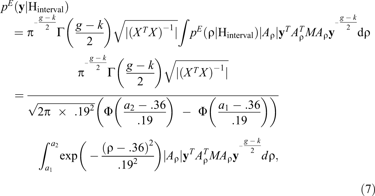
which is the aforementioned normal distribution with mean .36 and standard deviation .19, truncated to the corresponding parameter space of ρ under an interval hypothesis. The marginal likelihoods based on this empirical prior for ρ under precise and under interval hypotheses are given by (cf. Hepple 1995):

\begin{array}{l} p^{E} (y | H_{precise}) = π^{- \frac{g - k}{2}} Γ (\frac{g - k}{2}) \sqrt{| {(X^{T} X)}^{- 1} |} | A_{c} | y^{T} A_{c}^{T} M A_{c} y^{- \frac{g - k}{2}}, \end{array}

\begin{array}{l} p^{E} (y | H_{interval}) \\ = π^{- \frac{g - k}{2}} Γ (\frac{g - k}{2}) \sqrt{| {(X^{T} X)}^{- 1} |} \int p^{E} (ρ | H_{interval}) | A_{ρ} | y^{T} A_{ρ}^{T} M A_{ρ} y^{- \frac{g - k}{2}} dρ \\ = \frac{π^{- \frac{g - k}{2}} Γ (\frac{g - k}{2}) \sqrt{| {(X^{T} X)}^{- 1} |}}{\sqrt{2 π \times {.19}^{2}} (Φ (\frac{a_{2} - .36}{.19}) - Φ (\frac{a_{1} - .36}{.19}))} \int_{a_{1}}^{a_{2}} exp (- \frac{{(ρ - .36)}^{2}}{{.19}^{2}}) | A_{ρ} | y^{T} A_{ρ}^{T} M A_{ρ} y^{- \frac{g - k}{2}} d ρ, \end{array}

where $M : = I_{g} - X {(X^{T} X)}^{- 1} X^{T}$ and Φ(⋅) denotes the cumulative distribution function of the standard normal distribution.

The unidimensional integral in equation (7) does not have a closed-form solution and has to be evaluated numerically. This can be done by relying on standard numerical methods, for example, Simpson’s rule (Atkinson 1989), and we present R code therefor in Online Appendix A, allowing researchers to use the Bayes factor without having to deal with the formulae themselves. Subsequently, the desired Bayes factors are obtained through equation (4) by using the marginal likelihoods of the precise and interval hypotheses under consideration.

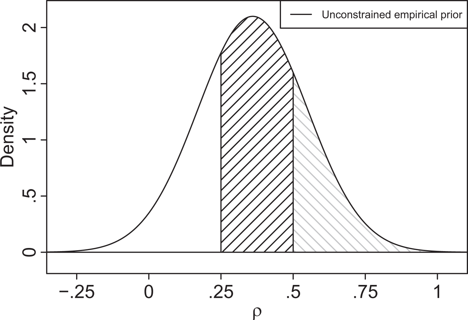
The unconstrained version of the empirical prior in equation (5), that is, $p (ρ) \sim N (.36, {.19}^{2})$ , can also be employed for determining prior probabilities of interval hypotheses. In this approach, the prior probabilities of the hypotheses are based on the probabilities of the tested model parameter falling in the respective intervals under a proper unconstrained prior. As an example, consider the two interval hypotheses $H_{1} : .25 < ρ \leq .5$ and $H_{2} : .5 < ρ < 1$ . The probabilities of ρ falling in the intervals (.25, .5] and (.5, 1) under the unconstrained empirical prior are equal to .49 and .23, respectively (see Figure 1).³ These probabilities give a quantification of the plausibility of the hypotheses under the unconstrained empirical prior. Hence, the corresponding prior odds, $p (H_{1}) / p (H_{2})$ , of the two hypotheses in this example is 2.12 (≈ .49/.23). In other words, under the empirical prior and before considering the data, a value of ρ inside the interval (.25, .5] is 2.12 times as likely as ρ being inside (.5, 1). Thus, if we assume that either H₁ or H₂ is true and that their prior odds corresponds to 2.12, the prior probabilities of the hypotheses are $p (H_{1}) = .68 (\approx .49 / (.49 + .23))$ and $p (H_{2}) = .32 (\approx .23 / (.49 + .23))$ . This seems reasonable as medium effects (H₁) are generally more plausible than large effects (H₂) in social network research (Dittrich et al. 2017). To the best of our knowledge, using an unconstrained prior for specifying prior odds of interval hypotheses is novel in the literature.⁴

Figure 1.

The probability density function of the unconstrained empirical prior for ρ, $p (ρ) \sim N (.36, {.19}^{2})$ . The areas of the shaded regions under the probability density function correspond to the probabilities of ρ falling in the interval (.25, .5] (black) and (.5, 1) (gray) which are equal to .49 and .23, respectively.

In the remainder of this article, we rely on the following method to assign prior model probabilities when testing one precise null hypothesis and T − 1 interval hypotheses.⁵ As there are T hypotheses in total, we set a prior probability of 1/T to the precise null hypothesis H₀. Subsequently, the remaining probability of (T − 1)/T is divided upon the interval hypotheses $H_{1},..., H_{T - 1}$ using the prior probabilities of the intervals under a proper unconstrained prior. For instance, consider $H_{0} : ρ = 0$ , $H_{1} : - .25 < ρ < 0$ , $H_{2} : 0 < ρ \leq .25$ , $H_{3} : .25 < ρ \leq .5$ , and $H_{4} : .5 < ρ < 1$ . Here, we test five hypotheses in total, so H₀ is assigned a prior probability of .2. The remaining probability of 4/5 = .8 is split between the four interval hypotheses based on the probability masses contained in the four intervals under the unconstrained empirical prior. For the hypotheses considered above, the probabilities of ρ falling in the respective intervals are $p (H_{1}) = .03$ , $p (H_{2}) = .25$ , $p (H_{3}) = .49$ , and $p (H_{4}) = .23$ . As we have already set $p (H_{0}) = .2$ , there is a total probability of .8 left for the remaining hypotheses. Rescaling and making them add up to .8 results in prior model probabilities of $H_{1}, H_{2}, H_{3}$ , and H₄ of .02, .20, .39, and .19.⁶ Finally, when combining the prior probabilities of the hypotheses and the marginal likelihoods in equations (6) and (7), the corresponding posterior model probabilities can be calculated via equation (2).

The Bayes Factor Based on a Uniform Prior

The uniform prior treats all possible network effects under the alternative(s) as equally likely before observing the data y, resulting in a flat prior distribution for ρ. As the region of support for ρ is bounded, the uniform prior for the network autocorrelation is a vague proper prior. Hence, it is less informative than the empirical prior but also does not represent complete prior ignorance which is typically expressed by using improper priors. The uniform prior under an interval hypothesis can be written as:

p^{U} (ρ | H_{interval}) \sim U (a_{1}, a_{2}),

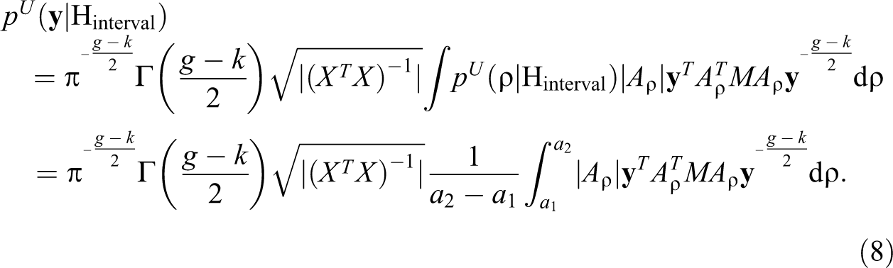
where $U (a_{1}, a_{2})$ denotes the uniform distribution on $(a_{1}, a_{2})$ . The marginal likelihood under H_precise remains the same as in equation (6), and the marginal likelihood under an interval hypothesis H_interval in combination with a uniform prior for ρ is now given by:

\begin{array}{l} p^{U} (y | H_{interval}) \\ = π^{- \frac{g - k}{2}} Γ (\frac{g - k}{2}) \sqrt{| {(X^{T} X)}^{- 1} |} \int p^{U} (ρ | H_{interval}) | A_{ρ} | y^{T} A_{ρ}^{T} M A_{ρ} y^{- \frac{g - k}{2}} dρ \\ = π^{- \frac{g - k}{2}} Γ (\frac{g - k}{2}) \sqrt{| {(X^{T} X)}^{- 1} |} \frac{1}{a_{2} - a_{1}} \int_{a_{1}}^{a_{2}} | A_{ρ} | y^{T} A_{ρ}^{T} M A_{ρ} y^{- \frac{g - k}{2}} dρ . \end{array}

Again, the Bayes factor is computed as the ratio of two marginal likelihoods under the uniform prior for ρ. Similarly as for the empirical prior, an unconstrained uniform prior can also be used for specifying prior model probabilities. In the uniform prior setting, this implies that the prior odds of two interval hypotheses is equal to the ratio of the lengths of the intervals. Posterior probabilities of the hypotheses can then be obtained via equation (2) and by plugging in the marginal likelihoods and prior probabilities of the hypotheses based on the uniform prior.

The Fractional Bayes Factor

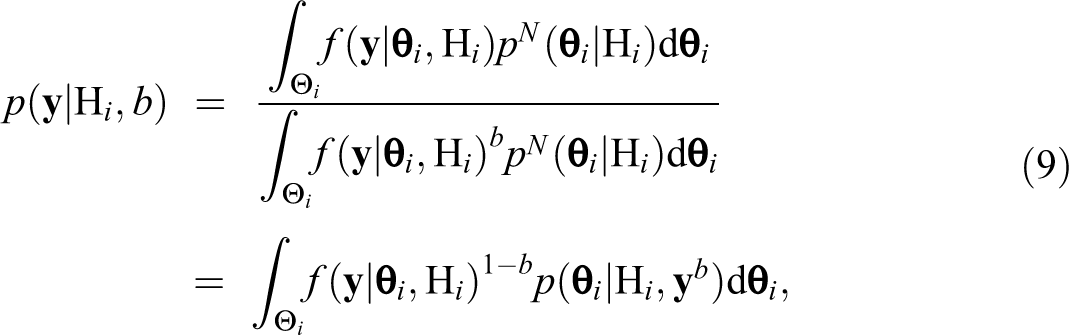
Finally, there may be situations where a researcher does not have any prior beliefs about possible network effects if the null would be false or where a researcher prefers not to specify a proper prior based on external knowledge. Such prior ignorance is usually reflected by employing improper priors. However, if improper priors for the tested parameters are imposed, the Bayes factor depends on unknown normalizing constants and is not well-defined (O’Hagan 1995). To that end, the fractional Bayes factor methodology was originally proposed by O’Hagan (1995) as a way to bypass this issue. In the fractional Bayes factor, the main idea is to split the information in the data into two different fractions that sum up to one. The first (small) fraction, denoted by b, is used for updating the initial improper prior into a proper default prior (Mulder 2014b); the second fraction, 1 − b, is taken for evaluating the hypotheses under investigation based on the default prior. In mathematical notation, this comes down to rewriting the marginal likelihood in equation (3) as:

\begin{matrix} p (y | H_{i}, b) = \frac{\int_{Θ_{i}} f (y | θ_{i}, H_{i}) p^{N} (θ_{i} | H_{i}) d θ_{i}}{\int_{Θ_{i}} f {(y | θ_{i}, H_{i})}^{b} p^{N} (θ_{i} | H_{i}) d θ_{i}} \\ = \int_{Θ_{i}} f {(y | θ_{i}, H_{i})}^{1 - b} p (θ_{i} | H_{i}, y^{b}) d θ_{i}, \end{matrix}

where $p^{N} (θ_{i} | H_{i})$ denotes a noninformative improper prior density for $θ_{i}$ under H_i and $p (θ_{i} | H_{i}, y^{b}) = f {(y | θ_{i}, H_{i})}^{b} p^{N} (θ_{i} | H_{i}) / \int_{Θ_{i}} f {(y | θ_{i}, H_{i})}^{b} p^{N} (θ_{i} | H_{i}) d θ_{i}$ is the updated, proper default prior. Thus, in order to compute the marginal likelihood in the network autocorrelation model in the fractional Bayes factor approach, one needs to choose a noninformative improper prior for ρ and to specify the fraction b. As improper prior for ρ we use,

p^{N} (ρ | H_{interval}) = {(1 - ρ)}^{- 1} 1_{(0, 1)} (ρ) .

This prior approximates the model’s independence Jeffreys prior very well (Online Appendix C), which has been shown to outperform the standard uniform prior for ρ in Bayesian estimation of the model (Dittrich et al. 2017).⁷ At the same time, the independence Jeffreys prior itself also imposes an a priori dependence structure between the model parameters (Dittrich et al. 2017), which makes it difficult to compare its inferences to those based on the based on the previously proposed normal and uniform marginal priors for ρ. For this reason, we rely on the marginal improper prior for ρ in equation (10) as it relaxes this a priori dependence. Note that in the fractional Bayes factor approach, we consider $H_{interval} : 0 < ρ < 1$ as the only alternative interval hypothesis. Else, if a researcher had more precise expectations about the magnitude of the network effect, for example, $.25 < ρ < .5$ , it seems much more sensible to use a proper prior for ρ instead.

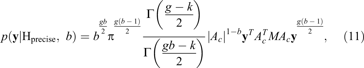
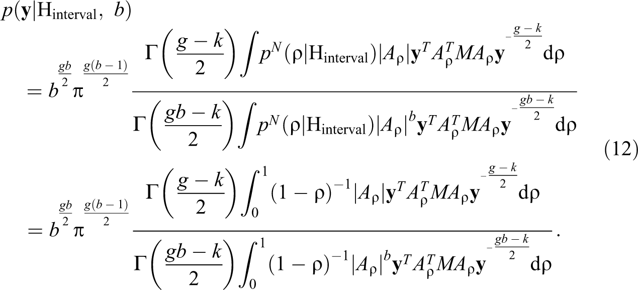
Typically, the fraction b in the fractional Bayes factor is chosen as the smallest value for which the updated default prior in equation (9) is proper (Berger and Mortera 1999; Mulder 2014b; O’Hagan 1995). This choice results in maximal possible use of the information in the data for hypothesis testing. If the proposed improper prior in equation (10) is combined with the standard noninformative prior for $(σ^{2}, β)$ , $p (σ^{2}, β) \propto 1 / σ^{2}$ , the corresponding updated prior in equation (9) is proper if b > k/g (see Online Appendix D for a proof). The proof shows that this also holds for the updated prior in equation (9) under H_precise. We denote the resulting choice for b as $b_{1} = (k + 1) / g$ . On the other hand, if misspecification of the improper prior is a concern, larger values for b may be preferred, as they can reduce the sensitivity of the fractional Bayes factor to prior misspecification (Conigliani and Anthony 2000; O’Hagan 1995). As empirical network autocorrelations are more likely to come from the estimated unconstrained population distribution for ρ in equation (5) than from a distribution that resembles the improper prior in equation (10), prior misspecification is indeed a valid concern. In this case, O’Hagan (1995) suggested to use $b_{2} = max (k + 1; ln (g)) / g$ , which makes the fractional Bayes factor more robust but increases slowly with g, or $b_{3} = max (k + 1; \sqrt{g}) / g$ , when sensitivity to misspecification of the prior is a serious concern. Finally, the marginal likelihoods under H_precise and H_interval in the fractional Bayes factor approach are given by:

\begin{array}{l} p (y | H_{precise}, b) = b^{\frac{g b}{2}} π^{\frac{g (b - 1)}{2}} \frac{Γ (\frac{g - k}{2})}{Γ (\frac{g b - k}{2})} | A_{c} |^{1 - b} y^{T} A_{c}^{T} M A_{c} y^{\frac{g (b - 1)}{2}}, \end{array}

\begin{matrix} p (y | H_{interval}, b) \\ = b^{\frac{g b}{2}} π^{\frac{g (b - 1)}{2}} \frac{Γ (\frac{g - k}{2}) \int p^{N} (ρ | H_{interval}) | A_{ρ} | y^{T} A_{ρ}^{T} M A_{ρ} y^{- \frac{g - k}{2}} dρ}{Γ (\frac{g b - k}{2}) \int p^{N} (ρ | H_{interval}) | A_{ρ} |^{b} y^{T} A_{ρ}^{T} M A_{ρ} y^{- \frac{g b - k}{2}} dρ} \\ = b^{\frac{g b}{2}} π^{\frac{g (b - 1)}{2}} \frac{Γ (\frac{g - k}{2}) \int_{0}^{1} {(1 - ρ)}^{- 1} | A_{ρ} | y^{T} A_{ρ}^{T} M A_{ρ} y^{- \frac{g - k}{2}} dρ}{Γ (\frac{g b - k}{2}) \int_{0}^{1} {(1 - ρ)}^{- 1} | A_{ρ} |^{b} y^{T} A_{ρ}^{T} M A_{ρ} y^{- \frac{g b - k}{2}} dρ} . \end{matrix}

For more technical details about the computation of equation (12), we refer the reader to Online Appendix E. As before, the marginal likelihoods in equations (11) and (12) are used to calculate the fractional Bayes factor itself, which is again the ratio of two marginal likelihoods. If a researcher is also interested in obtaining posterior model probabilities, a default choice is to impose equal prior model probabilities, that is, $p (H_{0}) = p (H_{1}) = .5$ , while subjective prior model probabilities could be assigned if a researcher has clear beliefs about the plausibility of the null hypothesis of a zero network effect.

Simulation Study

In this section, we present results of a simulation study investigating the performances of and the differences between the Bayes factors discussed in the fourth section. To that end, we first look at the one-sided test A: $H_{0} : ρ = 0$ versus $H_{1} : 0 < ρ < 1$ . In particular, we explore which Bayes factor converges fastest to the true hypothesis and assess the sensitivity of the fractional Bayes factor to the choice of b. Next, we consider a multiple hypothesis test B with a precise hypothesis and four interval hypotheses: $H_{0} : ρ = 0$ versus $H_{1} : - .25 < ρ < 0$ versus $H_{2} : 0 < ρ \leq .25$ versus $H_{3} : .25 < ρ \leq .5$ versus $H_{4} : .5 < ρ < 1$ . Our primary goal here is to study how fast the posterior model probabilities converge to the true model for different data-generating hypotheses and to check how robust these findings are to different marginal priors for ρ and to different prior model probabilities.

Study Design

In order to mimic realistic networks, we consider two different approaches for obtaining connectivity matrices W in test A. First, we use the well-known small-world structure (Watts and Strogatz 1998) to generate simulated networks. Such networks are highly clustered, that is, there is a tendency that network actors create very dense subnetworks but at the same time have small path lengths, that is, there is a high probability that any two actors in the network are connected by short paths of acquaintances (Watts and Strogatz 1998). Typically, this results in networks where most actors are linked to only a few others, while some actors, also known as hubs, have a lot of ties. These hubs function as connectors between different subnetworks and shorten the path length between two actors in the entire network. Small-world structures can be observed in online social networks (Fu et al. 2007), scientific collaboration networks (Newman 2001), or corporate elite networks (Davis, Yoo, and Baker 2003). We obtain simulated small-world networks relying on the “watts.strogatz.game” function from the igraph package in R (Version number is 1.0.1) (Csardi and Nepusz 2006). In the underlying algorithm, a ring lattice of g actors, each connected to its d nearest neighbors by undirected ties, is constructed first. Next, with probability r, each tie in the network is randomly rewired. Following Neuman and Mizruchi (2010) and Wang, Neuman, and Newman (2014), we set r = .1 that leads to highly clustered networks with low average path lengths. In our simulation study, we consider 14 network sizes $(g \in {25, 50, 75, 100, 150, 200, 300, ..., 1000})$ and two different mean degrees $(d \in {4, 8})$ . The simulated connectivity matrices are binary, that is, $W_{i j} = 1 (i, j \in {1, ..., g})$ if there is a tie between actor i and j and zero otherwise. Subsequently, we row-normalize the generated symmetric raw connectivity matrices.⁸

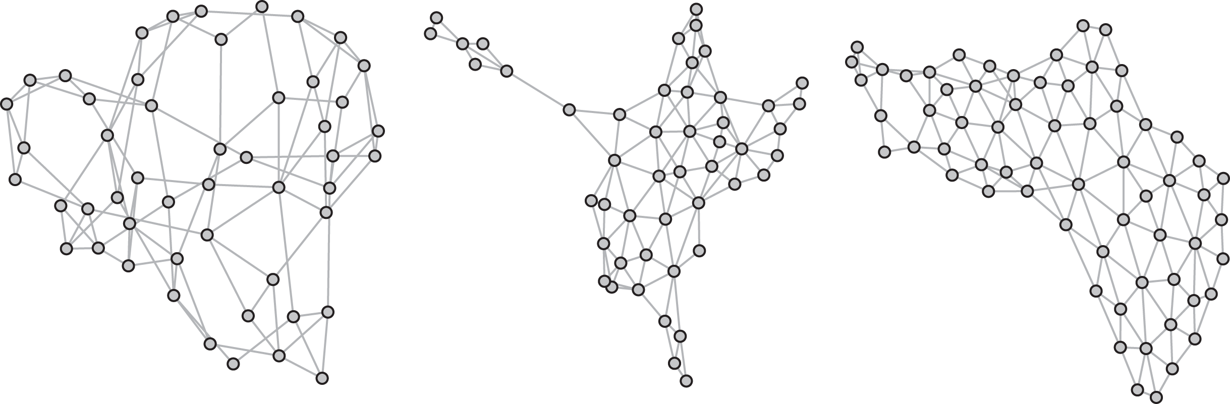
Second, we also run simulations using two prominent contiguity-based spatial networks; the 49 neighborhoods in Columbus, OH, analyzed in, for example, Anselin (1988), Elhorst (2014), and Hepple (1995) and the 64 Louisiana parishes studied in Doreian (1980), Howard (1971), and Leenders (2002), among others. In general, networks based on spatial proximity do not exhibit small-world properties, as there may be no short path between two distant nodes. Thus, we rely on these two real-world networks to gain insights into the behavior of the Bayes factors for network configurations that are different from typical small-world structures. We set $W_{i j} (i, j \in {1, ..., g})$ to one if area i is adjacent to area j, to zero otherwise, and row-standardize the raw adjacency matrices. Graphical representations of the two real networks and an example of a simulated small-world network appear in Figure 2.

Figure 2.

A simulated small-world network with g = 50, d = 4, r = .1 (left), the network of the 49 Columbus, OH, neighborhoods (middle), and the network of the 64 Louisiana parishes (right).

For each of the network types, we include three covariates plus an intercept term (so k = 4) and use three fixed levels for the network effect size $(ρ \in {0, .25, .5})$ to generate y via $y = {(I_{g} - ρ W)}^{- 1} (X β + ε)$ for test A. Furthermore, we also sample network effects from the estimated empirical population distribution from the estimated empirical population distribution of the network effects truncated to (0,1), rather than fixing ρ to a single-specific value. As the true network autocorrelation is unknown in practice, this is a more realistic setup than choosing specific values for ρ a priori. Finally, we draw independent values from a standard normal distribution for the elements of X (excluding the first column of X which is a vector of ones), β, and ε. Hence, we consider 120 scenarios (14 small-world networks × 2 mean degrees × 4 sampling schemes for ρ and 2 real networks × 4 sampling schemes for ρ) for test A in total and simulate 1,000 data sets for each scenario.

For test B, we generate network effects using the empirical prior for ρ, truncated to the corresponding parameter space under each hypothesis. We assign prior probabilities to each hypothesis based on the unconstrained versions of both the empirical and the uniform prior for ρ. We draw values for the elements of X, β, and ε as described in the previous paragraph, so for test B we examine 140 scenarios (14 small-world networks × 2 mean degrees × 5 data-generating hypotheses) in total, for which we generate 1,000 data sets for each.

Simulation Results

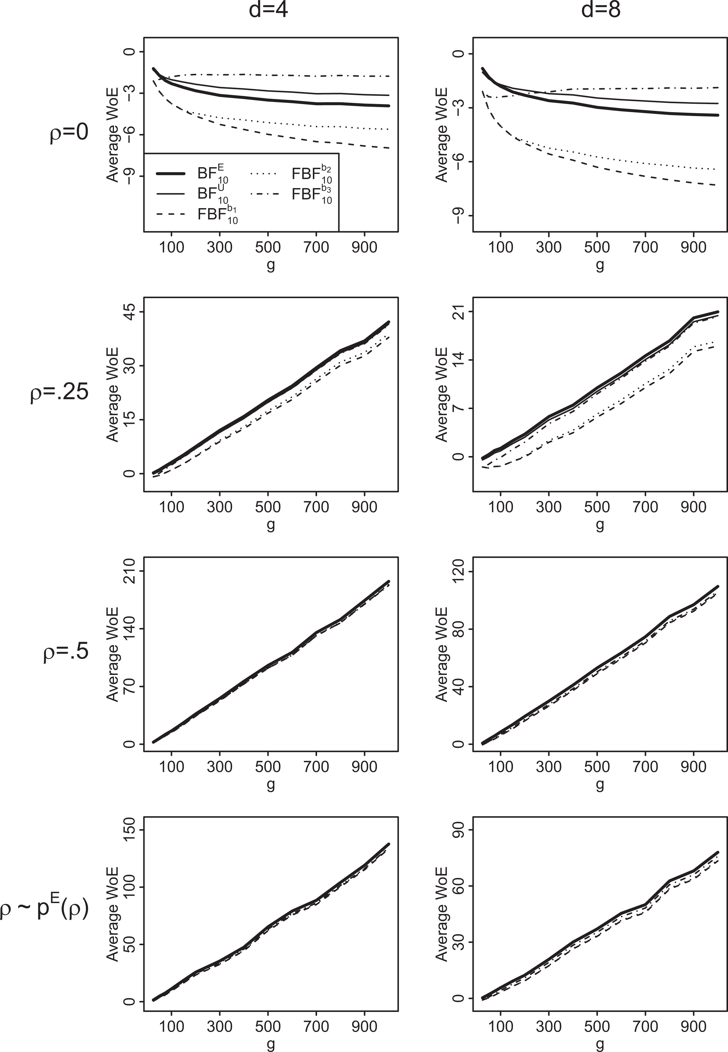
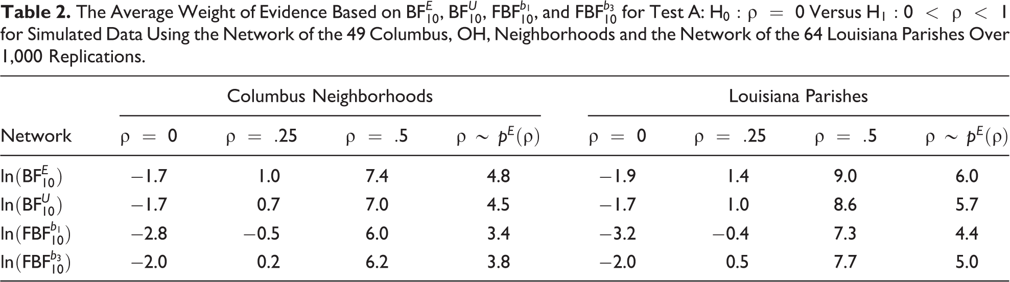
Figure 3 and Table 2 show the average weight of evidence, that is, the natural logarithm of the Bayes factor (Good 1985), for the different Bayes factors and network structures for test A: H₀ : ρ = 0 versus $H_{1} : 0 < ρ < 1$ .⁹

Figure 3.

The average weight of evidence based on ${BF}_{10}^{E}$ (thick solid line), ${BF}_{10}^{U}$ (thin solid line), ${FBF}_{10}^{b_{1}}$ (dashed line), ${FBF}_{10}^{b_{2}}$ (dotted line), and ${FBF}_{10}^{b_{3}}$ (dot-dashed line) for test A: $H_{0} : ρ = 0$ versus $H_{1} : 0 < ρ < 1$ for simulated data using generated small-world networks over 1,000 replications.

Table 2.

The Average Weight of Evidence Based on ${BF}_{10}^{E}$ , ${BF}_{10}^{U}$ , ${FBF}_{10}^{b_{1}}$ , and ${FBF}_{10}^{b_{3}}$ for Test A: $H_{0} : ρ = 0$ Versus $H_{1} : 0 < ρ < 1$ for Simulated Data Using the Network of the 49 Columbus, OH, Neighborhoods and the Network of the 64 Louisiana Parishes Over 1,000 Replications.

Network	Columbus Neighborhoods				Louisiana Parishes
Network	ρ = 0	ρ = .25	ρ = .5	$ρ \sim p^{E} (ρ)$	ρ = 0	ρ = .25	ρ = .5	$ρ \sim p^{E} (ρ)$
$ln ({BF}_{10}^{E})$	−1.7	1.0	7.4	4.8	−1.9	1.4	9.0	6.0
$ln ({BF}_{10}^{U})$	−1.7	0.7	7.0	4.5	−1.7	1.0	8.6	5.7
$ln ({FBF}_{10}^{b_{1}})$	−2.8	−0.5	6.0	3.4	−3.2	−0.4	7.3	4.4
$ln ({FBF}_{10}^{b_{3}})$	−2.0	0.2	6.2	3.8	−2.0	0.5	7.7	5.0

We can conclude the following from these results. First, the Bayes factor based on the empirical prior, ${BF}_{10}^{E}$ (thick solid line), and the Bayes factor based on the uniform prior, ${BF}_{10}^{U}$ (thin solid line), show consistent behavior, that is, the evidence for the true hypothesis is increasing with the network size. In addition, they almost always provide most evidence for the correct hypothesis, except for ρ = .25 and some smaller network sizes in the small-world networks. Second, the evidence for a true alternative hypothesis grows with the network size at a faster rate than the evidence for a true null as is common in other statistical models (Johnson and Rossell 2010) and for precise hypotheses in general. Third, the Bayes factor based on the empirical prior results in slightly even more evidence for a true hypothesis than the Bayes factor based on the uniform prior. Fourth, the smaller the mean degree, the bigger the evidence for a true alternative hypothesis provided by both ${BF}_{10}^{E}$ and ${BF}_{10}^{U}$ , for fixed g and ρ. This behavior is due to the negative bias of ρ in the model for increasing network densities (Mizruchi and Neuman 2008; Neuman and Mizruchi 2010; Smith 2009). Fifth, the fractional Bayes factors based on b₁ and b₂ (dashed line and dotted line) yield very similar results. Overall, they provide less evidence for the alternative hypothesis compared to ${BF}_{10}^{E}$ or ${BF}_{10}^{U}$ and appear to be biased toward the null. For example, this bias is manifested from the fact that networks of approximately 300 nodes are needed before the fractional Bayes factors based on b₁ and b₂ result in evidence for the true hypothesis H₁ when ρ equals .25 and d = 8 (see Figure 3). By way of comparison, the Bayes factors based on the empirical and the uniform prior already point toward evidence for the true alternative for small networks in this scenario. Sixth, the fractional Bayes factor based on b₃ (dot-dashed line) does not show consistent behavior when H₀ is true. In particular, the evidence for the true null hypothesis does not increase with the network size but remains constant or in some cases even decreases.

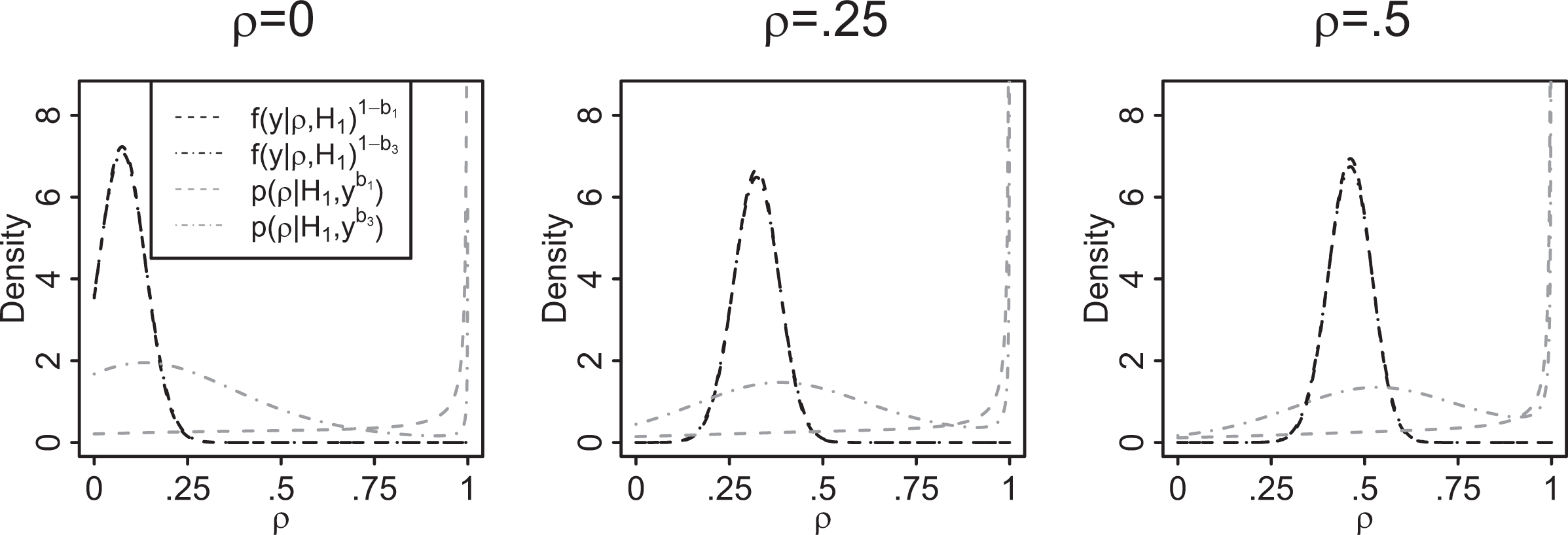
In order to provide more insights into the behavior of the fractional Bayes factor, we investigate its behavior more thoroughly. To that end, we observe that for small values of b, the updated marginal prior for ρ in the fractional Bayes factor approach in equation (9) is just proper with most of its probability mass still at values close to one for which the likelihood function is vanishing (see Figure 4). As the marginal likelihood under H₁ in the fractional Bayes factor approach is essentially an average weighted likelihood over (0, 1), with the updated prior acting as weight function, the fractional Bayes factors based on b₁ and b₂ tend to favor the null by construction. On the other hand, for large values of b, the updated marginal prior for ρ exhibits a local maximum near the maximum likelihood estimate of ρ (see Figure 4). When the data are generated under H₀, this results in a relatively larger average weighted likelihood over (0, 1) and considerable support for the alternative which explains the inconsistent behavior of the fractional Bayes factor based on the fraction b₃ when the null is true.

Figure 4.

The normalized integrated likelihood components $f {(y | ρ, H_{1})}^{1 - b_{1}}$ (black dashed line), $f {(y | ρ, H_{1})}^{1 - b_{3}}$ (black dot–dashed line), and the updated marginal priors $p (ρ | H_{1}, y^{b_{1}})$ (gray dashed line) and $p (ρ | H_{1}, y^{b_{3}})$ (gray dot–dashed line) under $H_{1} : 0 < ρ < 1$ based on $p^{N} (ρ | H_{1}) = {(1 - ρ)}^{- 1}$ for simulated data using generated small-world networks ( $g = 100, d = 8$ ). The integrated likelihood component and the updated marginal prior based on b₂ are not plotted, as they are graphically indistinguishable from the curves based on b₁.

Given the results from our simulation study, we recommend using the Bayes factor based on the empirical prior for ρ when testing $H_{0} : ρ = 0$ versus $H_{1} : 0 < ρ < 1$ or the Bayes factor based on the uniform prior as a second reasonable alternative. We do not recommend any of the fractional Bayes factors for this test, as they are either biased toward the null when the data are generated under the alternative or they show inconsistent behavior when H₀ is true. As a result, the fractional Bayes factors provide little improvement in classical null hypothesis significance testing, whereas the Bayes factors based on the empirical and uniform prior for ρ clearly do perform considerably well.

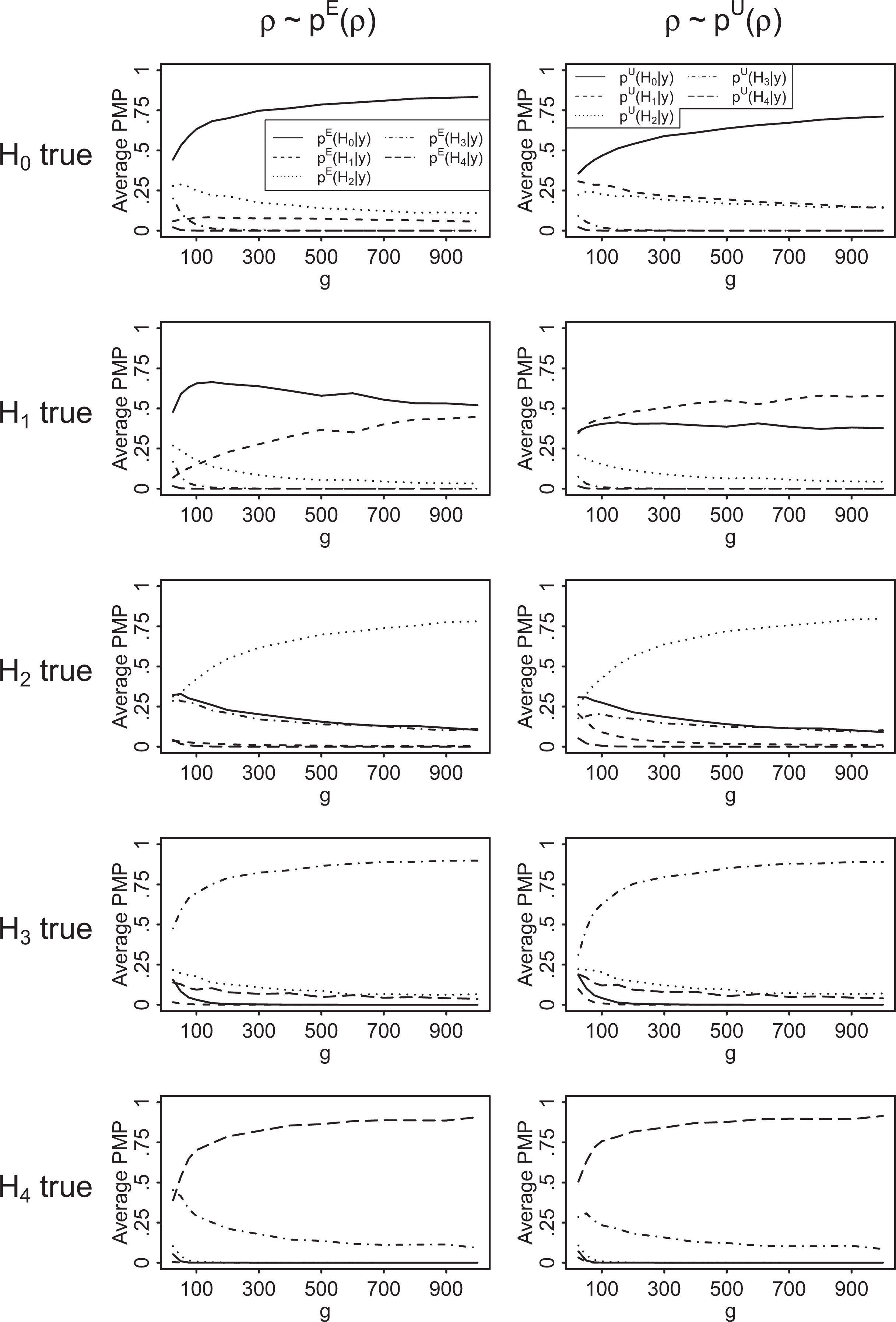
Figure 5 reports the average posterior model probabilities for test B based on the empirical prior, $p^{E} (H_{i} | y)$ , $i \in {0, 1, 2, 3, 4}$ (left column), and the ones based on the uniform prior, $p^{U} (H_{i} | y)$ (right column), for different network sizes and data-generating hypotheses.¹⁰

Figure 5.

The average posterior model probabilities of H₀ (solid line), H₁ (dashed line), H₂ (dotted line), H₃ (dot-dashed line), and H₄ (long-dashed line) for test B: $H_{0} : ρ = 0$ versus $H_{1} : - .25 < ρ < 0$ versus $H_{2} : 0 < ρ \leq .25$ versus $H_{3} : .25 < ρ \leq .5$ versus $H_{4} : .5 < ρ < 1$ , based on the empirical prior for ρ, $p^{E} (H_{i} | y), i \in {0, 1, 2, 3, 4}$ , (left column) and based on the uniform prior for ρ, $p^{U} (H_{i} | y)$ , (right column) for simulated data using generated small-world networks over 1,000 replications.

In general, for both $p^{E} (H_{i} | y)$ and $p^{U} (H_{i} | y)$ , the evidence for the true hypothesis is increasing with the sample size in all scenarios. Furthermore, the data-generating hypothesis always receives the most support, except for some very small network sizes and when the data are based on negative network effects in combination with the empirical prior. In the latter case, the prior probability of H₁, $p^{E} (H_{1}) = .02$ , is very small compared to the one of H₀, $p^{E} (H_{0}) = .20$ . This means that the data need to support H₁ approximately 10 times more than H₀ such that the hypotheses receive at least equal posterior probability. However, we believe this behavior of $p^{E} (H_{1} | y)$ not to be a real concern, as the empirical literature suggests that it is highly unlikely to observe negative values for ρ in practice (Dittrich et al. 2017). Else, if a researcher deems such negative network autocorrelations to be more plausible than implied by $p^{E} (H_{1}) = .02$ , H₁ should be accordingly given a higher prior probability.

Empirical Examples

In the following, we apply the Bayes factor based on the empirical prior for ρ to three data sets from the literature to quantify the relative evidence for different competing hypotheses of interest. We test the five hypotheses $H_{0} : ρ = 0$ , $H_{1} : - .25 < ρ < 0$ , $H_{2} : 0 < ρ \leq .25$ , $H_{3} : .25 < ρ \leq .5$ , and $H_{4} : .5 < ρ < 1$ against each other, corresponding to the notion of “no network effect,” a “minor negative network effect,” a “minor (positive) network effect,” a “medium network effect,” and a “large network effect,” respectively. We assign prior probabilities to these hypotheses using the unconstrained empirical prior from the fourth section, which yields $p^{E} (H_{0}) = .20$ , $p^{E} (H_{1}) = .02$ , $p^{E} (H_{2}) = .20$ , $p^{E} (H_{3}) = .39$ , and $p^{E} (H_{4}) = .19$ . In order to check robustness to the choice of the prior for ρ and to the choice of the prior model probabilities, we also perform our analyses using a uniform prior for the network autocorrelation parameter and for specifying prior model probabilities via the uniform unconstrained prior, that is, $p^{U} (H_{0}) = .20, p^{U} (H_{1}) = p^{U} (H_{2}) = p^{U} (H_{3}) = .16$ and $p^{U} (H_{4}) = .32$ . Finally, we compare the results to those coming from classical tests using p values.

Crime Data

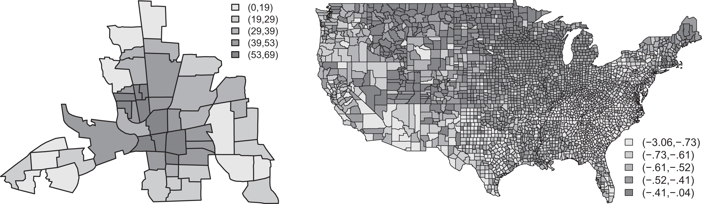
In the cross-sectional data set for 49 neighborhoods in Columbus, OH, first analyzed by Anselin (1988), the network autocorrelation model is used to explain the 1980 neighborhoods’ crime rates, operationalized as the combined total of residential burglaries and vehicle thefts per 1,000 households. This data set is openly accessible as part of the Columbus data from the R package spdep (Bivand and Piras 2015). Figure 6 (left panel) shows the spatial distribution of the crime rates across the 49 neighborhoods.

Figure 6.

The number of residential burglaries and vehicle thefts per 1,000 households across 49 neighborhoods in Columbus, OH, in 1980 (left), and the logarithm of voter turnout for the 1980 U.S. presidential election across 3,076 U.S. counties (right). The shading color of an entity indicates to which quintile of the sample it belongs.

Anselin (1988) modeled these crime rates as a function of household income and housing value (in 1,000USD$) plus an intercept term. In his study, both explanatory variables had a negative impact on the crime rate, while the maximum likelihood estimate of the network effect was ${\hat{ρ}}_{ML} = .40$ , with a 95 percent confidence interval for ρ of (.17; .64), and p = .0008.¹¹

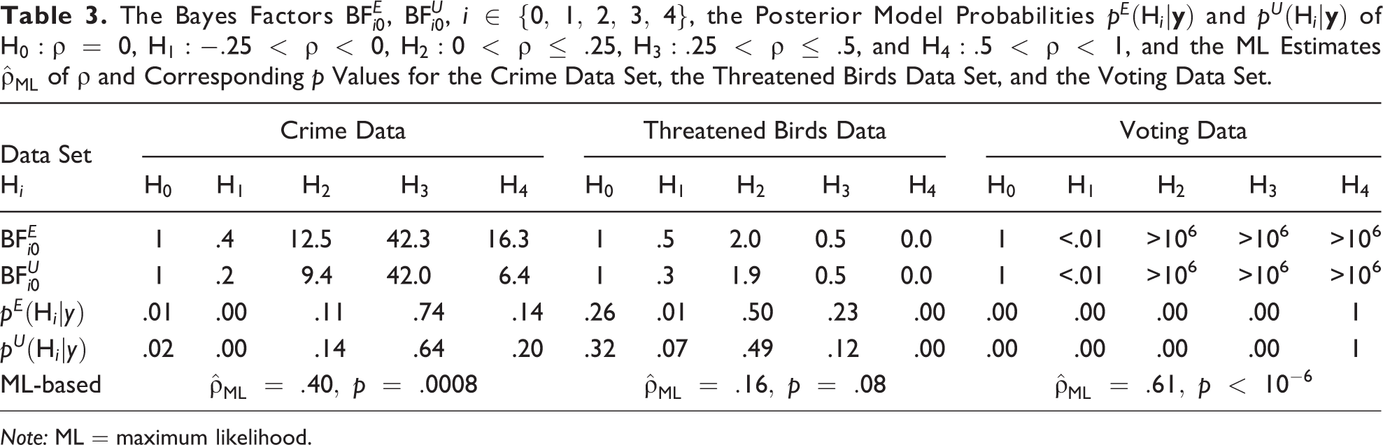
When using the empirical prior for ρ, the posterior probabilities of the hypotheses are $p^{E} (H_{0} | y) = .01$ , $p^{E} (H_{1} | y) = .00$ , $p^{E} (H_{2} | y) = .11$ , $p^{E} (H_{3} | y) = .74$ , and $p^{E} (H_{4} | y) = .14$ . In other words, H₃ is by far the most likely hypothesis and approximately 83 (≈ .74/.01), 1,744, 7, and 6 times more plausible than H₀, H₁, H₂, and H₄, respectively. Furthermore, the Bayes factor of H₃ versus H₀ is 42.3, which is considered as very strong evidence in the data for H₃, see Table 3, and the Bayes factor of H₃ versus H₄ (the second most supported hypothesis) is 2.6, which implies minor evidence for a medium effect relative to a large effect. R code for computing these posterior model probabilities and corresponding Bayes factors is provided in Online Appendix A. When relying on the uniform prior for ρ, the posterior model probabilities are $p^{U} (H_{0} | y) = .02$ , $p^{U} (H_{1} | y) = .00$ , $p^{U} (H_{2} | y) = .14$ , $p^{U} (H_{3} | y) = .64$ , and $p^{U} (H_{4} | y) = .20$ . Again, H₃ is by far the most likely hypothesis of the five, followed by H₄ which is approximately three times as unlikely as H₃. Thus, in line with the results from classical maximum likelihood–based inference, there is very strong evidence for a positive network effect. Contrary to maximum likelihood–based inference, however, the Bayesian approach also allows one to draw conclusions as to how much support there is in the data for particular values of ρ. In these data, evidence is strong that the network effect resides between .25 and .5, a conclusion that is affected neither by the choice of the prior for ρ nor by the choice of the prior model probabilities. Ultimately, among these Columbus neighborhoods, there is the most evidence for medium autocorrelation (between .25 and .5) with respect to crime rates. Table 3 summarizes the findings.

Table 3.

The Bayes Factors ${BF}_{i 0}^{E}$ , ${BF}_{i 0}^{U}$ , $i \in {0, 1, 2, 3, 4}$ , the Posterior Model Probabilities $p^{E} (H_{i} | y)$ and $p^{U} (H_{i} | y)$ of $H_{0} : ρ = 0$ , $H_{1} : - .25 < ρ < 0$ , $H_{2} : 0 < ρ \leq .25$ , $H_{3} : .25 < ρ \leq .5$ , and $H_{4} : .5 < ρ < 1$ , and the ML Estimates ${\hat{ρ}}_{ML}$ of ρ and Corresponding p Values for the Crime Data Set, the Threatened Birds Data Set, and the Voting Data Set.

Data Set	Crime Data					Threatened Birds Data					Voting Data
H_i	H₀	H₁	H₂	H₃	H₄	H₀	H₁	H₂	H₃	H₄	H₀	H₁	H₂	H₃	H₄
${BF}_{i 0}^{E}$	1	.4	12.5	42.3	16.3	1	.5	2.0	0.5	0.0	1	<.01	>10⁶	>10⁶	>10⁶
${BF}_{i 0}^{U}$	1	.2	9.4	42.0	6.4	1	.3	1.9	0.5	0.0	1	<.01	>10⁶	>10⁶	>10⁶
$p^{E} (H_{i} \| y)$	.01	.00	.11	.74	.14	.26	.01	.50	.23	.00	.00	.00	.00	.00	1
$p^{U} (H_{i} \| y)$	.02	.00	.14	.64	.20	.32	.07	.49	.12	.00	.00	.00	.00	.00	1
ML-based	${\hat{ρ}}_{ML} = .40, p = .0008$					${\hat{ρ}}_{ML} = .16, p = .08$					${\hat{ρ}}_{ML} = .61, p < 10^{- 6}$

Note: ML = maximum likelihood.

Threatened Birds Data

In the following example, McPherson and Nieswiadomy (2005) studied the percentage of threatened birds in 113 countries around the globe in the year 2000 via the network autocorrelation model, considering that “threats to a species in one country may spill over to neighboring countries’ species” (McPherson and Nieswiadomy 2005:401). In this data set, the spatial connectivity matrix was based on the shared border length between two neighboring countries which made several island countries isolates in the network.¹² In addition, the authors included 10, mainly socioeconomic, explanatory variables in the analysis plus an intercept term. The resulting maximum likelihood estimate of the network autocorrelation was ${\hat{ρ}}_{ML} = .16$ , with a 95 percent confidence interval for ρ of (−.06; .37), and p = .08, so “in other words, threats to birds spill over into adjoining countries” (McPherson and Nieswiadomy 2005:405).

Based on the empirical prior for ρ, the data yield posterior model probabilities of $p^{E} (H_{0} | y) = .26$ , $p^{E} (H_{1} | y) = .01$ , $p^{E} (H_{2} | y) = .50$ , $p^{E} (H_{3} | y) = .23$ , and $p^{E} (H_{4} | y) = .00$ . Hence, the hypothesis that there is a minor spillover effect of threats to birds across adjoining countries, that is, $H_{2} : 0 < ρ \leq .25$ , is most supported by the data and consequently results in the highest Bayes factor (see Table 3). However, the Bayes factor of a minor spillover effect relative to no spillover effect is only 2.0, so the support in the data for H₂ is far from decisive. In case of considering a uniform for ρ, the resulting posterior probabilities of the hypotheses are similar and given by $p^{U} (H_{0} | y) = .32$ , $p^{U} (H_{1} | y) = .07$ , $p^{U} (H_{2} | y) = .49$ , $p^{U} (H_{3} | y) = .12$ , and $p^{U} (H_{4} | y) = .00$ . Again, none of the alternative hypotheses receives convincing evidence to outweigh H₀. Overall, the data provide most evidence for ρ being between 0 and .25, but the Bayes factors also show that the strength of the evidence is rather small. These findings vividly illustrate the well-known issue that p values tend to overestimate the evidence against the null (Berger and Sellke 1987; Jeffreys 1961; Rouder et al. 2009; Sellke, Bayarri, and Berger 2001; Wagenmakers 2007).

Voting Data

The voting data set contains voter turnout for the 1980 U.S. presidential election from 3,107 U.S. counties. Pace and Barry (1997) employed a spatial Durbin model, a variant of the network autocorrelation model given by $y = ρ W y + α 1 + X β + W X γ + ε$ (where α denotes the model’s intercept term, 1 a vector of ones, and γ another vector of regression coefficients), to analyze the logarithm of the voter turnout (TURNOUT) across these U.S. counties.¹³ The spatial distribution of the logarithm of the voter turnout is shown in Figure 6 (right panel).¹⁴ As explanatory variables, the authors used the logarithms of, first, the population of 18 years of age or older eligible to vote in each county (POP); second, the population of 25 years of age or older with a twelfth grade or higher education in each county (EDUCATION); third, the number of owner-occupied housing units in each county (HOUSES); fourth, the aggregate income of each county (INCOME), and the four corresponding spatially lagged variables. Furthermore, the adjacency matrix W in this example was constructed on the basis of the four nearest neighbors of each county.¹⁵ Except for log(POP), and the spatially lagged log(HOUSES) and log(INCOME) variables, all other predictors were found to have a positive impact on log(TURNOUT), with a maximum likelihood estimate of ${\hat{ρ}}_{ML} = .62$ (Pace and Barry 1997:242), an associated 95 percent confidence interval for ρ of (.58; .65), and $p < 10^{- 6}$ .

Computing the corresponding posterior model probabilities underpins the decisive evidence for a large network effect, as $p^{E} (H_{0} | y) = .00$ , $p^{E} (H_{1} | y) = .00$ , $p^{E} (H_{2} | y) = .00$ , $p^{E} (H_{3} | y) = .00$ , and $p^{E} (H_{4} | y) = 1$ . Accordingly, the concomitant Bayes factor of H₄ versus any other considered hypothesis exceeds 10⁶ which provides “decisive” evidence in favor of H₄ compared to H₀, H₁, H₂, and H₃, respectively. When using the uniform prior, the posterior model probabilities remain essentially unchanged, as the evidence in the data for a large network effect is conclusive in this example. Although the implications of the Bayesian approach seem in line with the traditional approach, this is not the case completely: The only thing we can deduce from classical null hypothesis significance testing here is that we can reject the null hypothesis that ρ = 0. On the other hand, the Bayesian approach gives us much more detail about which values of ρ are most supported by the data and quantifies to what extent.

Conclusions

In this article, we developed three Bayes factors for testing precise and interval hypotheses for the network effect in the network autocorrelation model. The Bayesian approach to these tests comes with several practical advantages compared to classical null hypothesis significance testing. For instance, the Bayes factors and the resulting posterior model probabilities allow us to quantify the amount of evidence for a precise null hypothesis, or any other hypothesis, and they allow us to test multiple precise and interval hypotheses simultaneously without any of the drawbacks of classical null hypothesis significance testing. We ran an extensive simulation study to evaluate the numerical behavior of the presented Bayes factors for a wide range of different network configurations. We found that the Bayes factor based on an empirical prior for the network effect—relying on a summary of published network autocorrelations from many different sources—is always consistent, displays superior performance, and is the Bayes factor we recommend. At the same time, using a uniform prior for ρ instead yields properties that are almost as good as those based on the empirical prior. Finally, we do not recommend employing improper priors for ρ in combination with the fractional Bayes factor methodology. We illustrated the practical use of the recommended Bayes factors with three examples and provided computer code in R, making the proposed Bayes factors easily available to researchers interested in testing for the existence and magnitude of a network effect in the network autocorrelation model.

Given the importance of the network autocorrelation model in a wide variety of fields, we believe there is much value to having available an approach that makes it possible for researchers to test hypotheses that go beyond the standard significance test $H_{0} : ρ = 0$ versus $H_{1} : ρ \neq 0$ which is only useful for falsifying the null. The new Bayesian tests provide means for quantifying evidence in favor of any hypothesis and enable researchers to test multiple hypotheses against one another in a single analysis including, but not restricted to, any combination of precise and interval hypotheses. Overall, we hope that these tools will enrich the tool kit of researchers studying network effects through the network autocorrelation model.

Supplemental Material

Online_Appendices - Network Autocorrelation Modeling: A Bayes Factor Approach for Testing (Multiple) Precise and Interval Hypotheses

Online_Appendices for Network Autocorrelation Modeling: A Bayes Factor Approach for Testing (Multiple) Precise and Interval Hypotheses by Dino Dittrich, Roger Th. A. J. Leenders and Joris Mulder in Sociological Methods & Research

Footnotes

Acknowledgment

We thank Michael A. McPherson and Michael L. Nieswiadomy for sharing their data with us.

Declaration of Conflicting Interests

The author(s) declared no potential conflicts of interest with respect to the research, authorship, and/or publication of this article.

Funding

The author(s) disclosed receipt of the following financial support for the research, authorship, and/or publication of this article: The third author was supported by a Veni Grant (016.145.205) provided by The Netherlands Organization for Scientific Research.

Supplemental Material

Supplemental material for this article is available online.

Notes

References

Anselin

1982. “A Note on Small Sample Properties of Estimators in a First-order Spatial Autoregressive Model.” Environment and Planning A 14:1023–30.

Anselin

. 1988. Spatial Econometrics: Methods and Models. Dordrecht, the Netherlands: Kluwer Academic.

Anselin

2002. “Under the Hood: Issues in the Specification and Interpretation of Spatial Regression Models.” Agricultural Economics 27:247–67.

Atkinson

K. E

. 1989. An Introduction to Numerical Analysis. 2nd ed. New York: Wiley.

Baller

R. D.

Anselin

Messner

S. F.

Deane

Hawkins

D. F.

. 2001. “Structural Covariates of U.S. County Homicide Rates: Incorporating Spatial Effects.” Criminology 39:561–88.

Berger

J. O.

Mortera

. 1999. “Default Bayes Factors for Nonnested Hypothesis Testing.” Journal of the American Statistical Association 94:542–54.

Berger

J. O.

Sellke

. 1987. “Testing a Point Null Hypothesis: The Irreconcilability of P Values and Evidence.” Journal of the American Statistical Association 82:112–22.

Beck

Gleditsch

K. S.

Beardsley

. 2006. “Space Is More than Geography: Using Spatial Econometrics in the Study of Political Economy.” International Studies Quarterly 50:27–44.

Becker

Richard A.

Brownrigg

Ray

Minka

Thomas P.

Wilks

Allen. R.

Deckmyn

. 2016. Maps: Draw Geographical Maps. R Package Version 3.1.1 (https://cran.r-project.org/web/packages/maps/maps.pdf).

10.

Bivand

Piras

. 2015. “Comparing Implementations of Estimation Methods for Spatial Econometrics.” Journal of Statistical Software 63:1–36.

11.

Braeken

Mulder

Wood

. 2015. “Relative Effects at Work: Bayes Factors for Order Hypotheses.” Journal of Management 41:544–73.

12.

Casella

Girón

F. J.

Martínez

M. L.

Moreno

. 2009. “Consistency of Bayesian Procedures for Variable Selection.” The Annals of Statistics 37:1207–28.

13.

Conigliani

Anthony

. 2000. “Sensitivity of the Fractional Bayes Factor to Prior Distributions.” The Canadian Journal of Statistics 28:343–52.

14.

Csardi

Nepusz

. 2006. “The Igraph Software Package for Complex Network Research.” InterJournal, Complex Systems:1695. (https://cran.r-project.org/web/packages/igraph/citation.html).

15.

Davis

G. F.

Yoo

Baker

W. E.

. 2003. “The Small World of the American Corporate Elite, 1982–2001.” Strategic Organization 1:301–26.

16.

De Oliveira

Song

J. J.

. 2008. “Bayesian Analysis of Simultaneous Autoregressive Models.” Sankhya: The Indian Journal of Statistics, Series B (2008-) 70:323–50.

17.

Dittrich

Leenders

R. T.

Mulder

. 2017. “Bayesian Estimation of the Network Autocorrelation Model.” Social Networks 48:213–36.

18.

Doreian

1980. “Linear Models with Spatially Distributed Data: Spatial Disturbances or Spatial Effects?” Sociological Methods & Research 9:29–60.

19.

Duke

J. B.

1993. “Estimation of the Network Effects Model in a Large Data Set.” Sociological Methods & Research 21:465–81.

20.

Elhorst

J. P

. 2014. Spatial Econometrics: From Cross-sectional Data to Spatial Panels. Berlin: Springer.

21.

Chen

Liu

Wang

. 2007. “Social Dilemmas in an Online Social Network: The Structure and Evolution of Cooperation.” Physics Letters A 371:58–64.

22.

Gelman

Carlin

J. B.

Stern

H. S.

Dunson

D. B.

Vehtari

Rubin

D. B.

. 2013. Bayesian Data Analysis. 3rd ed. Boca Raton: Chapman & Hall/CRC.

23.

Gimpel

Schuknecht

. 2003. “Political Participation and the Accessibility of the Ballot Box.” Political Geography 22:471–88.

24.

Good

1985. “Weight of Evidence: A Brief Survey.” Pp. 249–69 in Bayesian Statistics 2, edited by Bernardo

J. M.

DeGroot

M. H.

Lindley

D. V.

New York: North-Holland

A. Smith.

25.

Mulder

Deković

Hoijtink

. 2014. “Bayesian Evaluation of Inequality Constrained Hypotheses.” Psychological Methods 19:511–27.

26.

Han

Lee

L. -F.

. 2013. “Bayesian Estimation and Model Selection for Spatial Durbin Error Model with Finite Distributed Lags.” Regional Science and Urban Economics 43:816–37.

27.

Hepple

L. W.

1979. “Bayesian Analysis of the Linear Model with Spatial Dependence.” Pp. 179–99 in Exploratory and Explanatory Statistical Analysis of Spatial Data, edited by Bartels

C. P.

Ketellapper

. Dordrecht, the Netherlands: Springer.

28.

Hepple

L. W.

1995. “Bayesian Techniques in Spatial and Network Econometrics: 1. Model Comparison and Posterior Odds.” Environment and Planning A 27:447–69.

29.

Holloway

Shankar

Rahman

. 2002. “Bayesian Spatial Probit Estimation: A Primer and an Application to Hyv Rice Adoption.” Agricultural Economics 27:383–402.

30.

Howard

P. H

. 1971. Political Tendencies in Louisiana. Baton Rouge: Louisiana State University Press.

31.

Jeffreys

. 1961. Theory of Probability. 3rd ed. Oxford: Oxford University Press.

32.

Johnson

V. E.

Rossell

. 2010. “On the Use of Non-local Prior Densities in Bayesian Hypothesis Tests.” Journal of the Royal Statistical Society: Series B (Statistical Methodology) 72:143–70.

33.

Kass

R. E.

Raftery

A. E.

. 1995. “Bayes Factors.” Journal of the American Statistical Association 90:773–95.

34.

Kirk

D. S.

Papachristos

A. V.

. 2011. “Cultural Mechanisms and the Persistence of Neighborhood Violence.” American Journal of Sociology 116:1190–233.

35.

Klugkist

Laudy

Hoijtink

. 2005. “Inequality Constrained Analysis of Variance: A Bayesian Approach.” Psychological Methods 10:477–93.

36.

Kuha

2004. “AIC and BIC: Comparisons of Assumptions and Performance.” Sociological Methods & Research 33:188–229.

37.

Leenders

R. T.

1995. “Structure and Influence: Statistical Models for the Dynamics of Actor Attributes, Network Structure and Their Interdependence.” PhD thesis, Thesis Publishers, Amsterdam, the Netherlands.

38.

Leenders

R. T.

2002. “Modeling Social Influence through Network Autocorrelation: Constructing the Weight Matrix.” Social Networks 24:21–47.

39.

LeSage

J. P.

1997. “Bayesian Estimation of Spatial Autoregressive Models.” International Regional Science Review 20:113–29.

40.

LeSage

J. P.

Parent

. 2007. “Bayesian Model Averaging for Spatial Econometric Models.” Geographical Analysis 39:241–67.

41.

Liu

C. C.

Aitkin

. 2008. “Bayes Factors: Prior Sensitivity and Model Generalizability.” Journal of Mathematical Psychology 52:362–75.

42.

Marsden

P. V.

Friedkin

N. E.

. 1993. “Network Studies of Social Influence.” Sociological Methods & Research 22:127–51.

43.

McMillen

D. P.

2010. “Issues in Spatial Data Analysis.” Journal of Regional Science 50:119–41.

44.

McPherson

M. A.

Nieswiadomy

M. L.

. 2005. “Environmental Kuznets Curve: Threatened Species and Spatial Effects.” Ecological Economics 55:395–407.

45.

Mizruchi

M. S.

Neuman

E. J.

. 2008. “The Effect of Density on the Level of Bias in the Network Autocorrelation Model.” Social Networks 30:190–200.

46.

Mizruchi

M. S.

Stearns

L. B.

Marquis

. 2006. “The Conditional Nature of Embeddedness: A Study of Borrowing by Large US Firms, 1973-1994.” American Sociological Review 71:310–33.

47.

Mulder

(2014a). “Bayes Factors for Testing Inequality Constrained Hypotheses: Issues with Prior Specification.” British Journal of Mathematical and Statistical Psychology 67:153–71.

48.

Mulder

(2014b). “Prior Adjusted Default Bayes Factors for Testing (in)Equality Constrained Hypotheses.” Computational Statistics and Data Analysis 71:448–63.

49.

Mulder

Klugkist

van de Schoot

Meeus

W. H.

Selfhout

Hoijtink

. 2009. “Bayesian Model Selection of Informative Hypotheses for Repeated Measurements.” Journal of Mathematical Psychology 53:530–46.

50.

Mulder

Wagenmakers

E.-J.

. 2016. “Editors Introduction to the Special Issue “Bayes Factors for Testing Hypotheses in Psychological Research: Practical Relevance and New Developments.”” Journal of Mathematical Psychology 72:1–5.

51.

Mur

López

Angulo

. 2008. “Symptoms of Instability in Models of Spatial Dependence.” Geographical Analysis 40:189–211.

52.

Neuman

E. J.

Mizruchi

M. S.

. 2010. “Structure and Bias in the Network Autocorrelation Model.” Social Networks 32:290–300.

53.

Newman

M. E.

2001. “The Structure of Scientific Collaboration Networks.” Proceedings of the National Academy of Sciences of the United States of America 98:404–09.

54.

O’Hagan

1995. “Fractional Bayes Factors for Model Comparison.” Journal of the Royal Statistical Society. Series B (Statistical Methodology) 57:99–138.

55.

Ord

1975. “Estimation Methods for Models of Spatial Interaction.” Journal of the American Statistical Association 70:120–26.

56.

Pace

R. K.

Barry

. 1997. “Quick Computation of Spatial Autoregressive Estimators.” Geographical Analysis 29:232–47.

57.

Raftery

A. E.

Madigan

Hoeting

J. A.

. 1997. “Bayesian Model Averaging for Linear Regression Models.” Journal of the American Statistical Association 92:179–91.

58.

Rouder

J. N.

Speckman

P. L.

Sun

Morey

R. D.

Iverson

. 2009. “Bayesian t Tests for Accepting and Rejecting the Null Hypothesis.” Psychonomic Bulletin & Review 16:225–37.

59.

Sellke

Bayarri

Berger

J. O.

. 2001. “Calibration of p Values for Testing Precise Null Hypotheses.” The American Statistician 55:62–71.

60.

Sewell

D. K.

2017. “Network Autocorrelation Models with Egocentricdata.” Social Networks 49:113–23.

61.

Shaffer

J. P.

1995. “Multiple Hypothesis Testing.” Annual Review of Psychology 46:561–84.

62.

Sinharay

Stern

H. S.

. 2002. “On the Sensitivity of Bayes Factors to the Prior Distributions.” The American Statistician 56:196–201.

63.

Smith

T. E.

2009. “Estimation Bias in Spatial Models with Strongly Connected Weight Matrices.” Geographical Analysis 41:307–32.

64.

Tita

G. E.

Radil

S. M.

. 2011. “Spatializing the Social Networks of Gangs to Explore Patterns of Violence.” Journal of Quantitative Criminology 27:521–45.

65.

Wagenmakers

E.-J.

2007. “A Practical Solution to the Pervasive Problems of p Values.” Psychonomic Bulletin & Review 14:779–804.

66.

Wang

Neuman

E. J.

Newman

D. A.

. 2014. “Statistical Power of the Social Network Autocorrelation Model.” Social Networks 38:88–99.

67.

Watts

D. J.

Strogatz

S. H.

. 1998. “Collective Dynamics of “Small-world Networks”.” Nature 393:440–442.

68.

Weakliem

D. L.

2004. “Introduction to the Special Issue on Model Selection.” Sociological Methods & Research 33:167–87.

69.

Wetzels

Wagenmakers

E.-J.

. 2012. “A Default Bayesian Hypothesis Test for Correlations and Partial Correlations.” Psychonomic Bulletin & Review 19:1057–64.

Supplementary Material

Please find the following supplemental material available below.

For Open Access articles published under a Creative Commons License, all supplemental material carries the same license as the article it is associated with.

For non-Open Access articles published, all supplemental material carries a non-exclusive license, and permission requests for re-use of supplemental material or any part of supplemental material shall be sent directly to the copyright owner as specified in the copyright notice associated with the article.

0.00 MB

0.28 MB