Two-sample Age-period-cohort Models

Abstract

Age-period-cohort analysis is often done in the context of two samples. This could be samples for women and men or for two countries. It is of interest to ask if some time effects could be common across samples. We clarify how the well-known age-period-cohort problem for one sample carries over to the two sample situation. This is done through a reparametrization in terms of parameters that are invariant to the identification issues. The new parametrization shows which hypotheses can be tested and their degrees of freedom. Testable hypotheses can be formulated for non-linear effects, but not for the linear parts of the individual time effects. This conclusion remains when imposing cross-sample restrictions. The analysis is extended to the mixed frequency situation where age and period are measured at different scales. As an empirical illustration a study of Swiss suicide rates is revisited.

Introduction

It is common to have data in the form of two age-period tables, for instance for women and for men. Investigators often fit age-period-cohort models to each table and then compare the time affects across samples. For instance a common period effect could be attributable to societal effects. It is unclear from the literature, how the usual age-period-cohort problem for a single sample carries over to the two-sample case. The purpose of this paper is to clarify this.

Two-sample data. We will revisit a study of Swiss suicide rates (Riebler et al. 2012). The data consists of rates by age, period and sex. Suicide rates tend to increase with age and to be higher for men than for women. The rates vary by period and by birth cohort, quite possibly due to time-varying socio-economic factors. Disentangling these various effects from time, sex and society, could be helpful in work to prevent suicides. A two-sample age-period-cohort model is well-suited for this, but we need to know what hypotheses entail and what the associated degrees of freedom are. The data has the additional challenge that age is measured on a five-year scale while period is annual. We will consider how this changes the age-period-cohort problem.

Some other two-sample examples are the following. Riebler and Held (2010) compared female mortality in Danmark and Norway. Dinas and Stoker (2014) compared male and female participation rates in US presidential elections after the introduction of universal suffrage. Cairns et al. (2011) investigated selection effects in life insurance. Fannon et al. (2021) analyzed obesity for English women and men using repeated cross sections. In all these examples it is of interest to formulate and investigate hypotheses about common age, period or cohort effects.

The age-period-cohort problem for two-sample models is similar to the standard problem for one sample The essence of the one-sample problem is as follows. Age, period and cohort effects are functions of time. Each function has a linear part and a non-linear part. The age-period-cohort problem is that the aggregate of the age, period and cohort effects does not change by adding an arbitrary linear trend to each of the age and cohort effects while subtracting it from the period effect. It has long been understood that such linear manipulations change the linear parts of the individual time effects, while leaving non-linear parts unaltered. There is a vast literature on these issues and what to do about them. An early reference is Fienberg and Mason (1979). Kuang et al. (2008) noted that the linear parts of the age, period and cohort effects combine to a linear plane, which is also unchanged under linear manipulations. Further, the degrees of freedom of the model matches exactly the degrees of freedom of the non-linear parts plus the degrees of freedom of the linear plane. Thus, all statistical estimation and inference should be concerned with the non-linear parts and the linear plane and only that. All hypotheses on the individual linear parts are untestable.

What constitutes the individual linear parts of a model can be confusing. This point was made by Clayton and Schifflers (1987), see Fannon and Nielsen (2019) for a recent review and the comment of Keiding and Andersen (2016) on an empirical analysis linking maternal age with offspring outcomes. To appreciate this point, consider the extreme restriction where the age-period-cohort effects combine to zero for all ages and periods. While this model has no parameters and no statistical tools are needed, the age-period-cohort problem remains. The restriction stipulates that the individual effects add up to zero. It may be true that each of the age, period and cohort effects is zero. Equally, we can add a linear trend to each of the age and cohort effects if we also subtract it from the period effect. But, there are no degrees of freedom left to learn about this.

The age-period-cohort problem comprises two problems. The primary problem is of invariance. We must avoid getting confused by pernicious manipulations of the linear parts of the individual effects. We do that by focussing on the non-linear parts and the linear plane, which are unaffected by the manipulations. Mathematically, we say that these parts are ‘invariant’ to the age-period-cohort problem. The secondary problem is of identification or collinearity.

There is a lively debate about what to do about the age-period-cohort problem. This arises because we can solve the identification problem without addressing the invariance problem. Broadly speaking, there appears to be three approaches. First, one can impose constraints on the time effects to achieve identification without getting invariance. One can set a subset of the time effect parameters to zero as discussed by Fienberg and Mason (1979). More elaborate suggestions are given by Fosse and Winship (2019), Fu (2018), O’Brien (2022), Yang and Land (2013) for one-sample models, by Riebler and Held (2010) for two-sample models, and by Fu (2018), Gascoigne and Smith (2023), Riebler and Held (2010), Yang and Land (2006) for mixed frequency models. Some of these choices have attracted considerable discussion, see for instance Bell and Jones (2015), Luo (2013), Luo and Hodges (2016), Nielsen and Nielsen (2014), O’Brien (2011), Reither et al. (2015). Second, as suggested by Chauvel and Schröder (2014), Clayton and Schifflers (1987), Fienberg and Mason (1979), Holford (1983), McKenzie (2006), Rosenberg (2019), one can apply the first approach for estimation and then extract estimates for invariant functions. Third, one can reparametrize the predictor exclusively in terms of invariant parameters. This requires a mathematical representation of the predictor in terms of the invariant parameters. As a result, the age-period-cohort model can be approached as any other regression problem. This approach was proposed in (Kuang et al. 2008). See also (Smith and Wakefield 2016) for a Bayesian implementation, (Fannon and Nielsen 2019) for reviews and (Billari and Graziani 2023) for a recent fertility application. We will extend the invariance approach to the two-sample model.

The two-sample model. For two samples, the immediate issue is to generalize the description of the age-period-cohort problem. The generalization essentially amounts to adding an index for sample. The immediate consequence is that for each sample, the non-linear parts of the individual effects and the linear plane are invariant, whereas the linear parts of the individual effects change by linear manipulations. It follows that restrictions on the non-linear parts and the linear planes within samples or across samples are testable. But, by analogy with the above zero model argument, all hypotheses on the individual linear parts within samples or across samples are untestable.

When the data also have a mixed-frequency structure, the age-period-cohort problem is more involved. For instance, suppose age is grouped in five year intervals while the period is annual as in the Swiss data. Then the cohort effects related to the age-group 25–29, say, will be different in two consecutive periods due to a one-year shift. Rather, the cohort effects for the 25–29 age-group are only repeated for the 30–34 age group five periods later. Thus, the non-linear effects and linear planes have to be formed with some care to include ‘macro’ 5-year steps and ‘micro’ 1-year shifts. Key references are Holford (2006) and Riebler and Held (2010), who describe macro and micro effects. Recently, Nielsen (2022) has used the invariance approach to give a complete characterization of the mixed frequency identification problem for one sample with an arbitrary mixed-frequency structure. We extend that analysis to the two-sample situation.

The analysis of the parametrization is applicable in a broad range of statistical models. This includes generalized linear models whether they are based on the normal, the Poisson or the binomial distributions. It is applicable to aggregate tables and to repeated cross-sectional data. It will be applicable to panel data with some modification. In a particular application, the user will have to decide how to conduct inference. This problem will be addressed in the context of the empirical illustration.

The empirical illustration uses the Swiss data with suicide rates for women and men. We will employ a statistical model where log rates are normal. In so far as one is interested in analyzing the sexes separately through one-sample analyses, standard exact normal inference works, so that t-tests are t-distributed and F-tests are F-distributed. However, this does not extend to cross-sample analysis as suicide rates are 2-2.5 times larger for men than for women, so that error variances differ for the two samples. In this situation, the exact normal inference is no longer available. Instead we will rely on the recent small-dispersion inference developed in Harnau and Nielsen (2018); Kuang and Nielsen (2020).

A practical advice is that substantive questions should be linked to the non-linear parts of the age, period and cohort effects and to linear planes only. The non-linear effects will typically be of most interest. They can be expressed in terms of differences of differences of the time effects. In many situations this may actually be rather natural. For instance, in logistic models, this amounts to log odds ratios which are the usual object of interest. The differences of differences will have a relatively simple form with regularly spaced time scales and a more complicated form with mixed frequency data. When it comes to estimating and testing restrictions, one can with advantage use the proposed parametrization in a regression framework as it allows for easy estimation of both the unrestricted model and any restricted sub-models.

Outline. Section ‘Motivation: the Swiss Suicide Data’ presents the Swiss data. The two-sample age-period-cohort problem is analyzed for regular data in Section ‘The Two-sample Model for Regular Data’ and for mixed-frequency data in Section ‘The Two-sample Model for Mixed Data’. Section ‘Empirical Illustration’ gives the empirical illustration. An online supplement contains an appendix with technical aspects and replication materials using the R-package apc (Nielsen 2015).

Motivation: the Swiss Suicide Data

We consider the Swiss suicide data presented and analyzed by Riebler et al. (2012). The data consists of suicide mortality counts and mid-year population data organized as two mixed-frequency age-period arrays for women and men. Age is grouped in five year intervals 15–19,…,75–79 while period is annual for 1950–2007. Thus, there are 13 age groups covering a 65 year range and 58 annual periods. In the present data, the counts range from 5 to 54 for women with a median of 27. For men, the range is 18–133 with a median of 66.

Figure 1 shows crude suicide rates by age and period for women and men. The crude rates are found as the sum of all mortality counts for a given age or period divided by the sum of the population data and standardized as rates per 100,000 people. The rates increase with age while female rates are about a third of the male rates. The rates per period fall through the 1950s and 1960s, then increase through the 1970s, after which they fall back again. The peak could match socio-economic trends.

Figure 1.

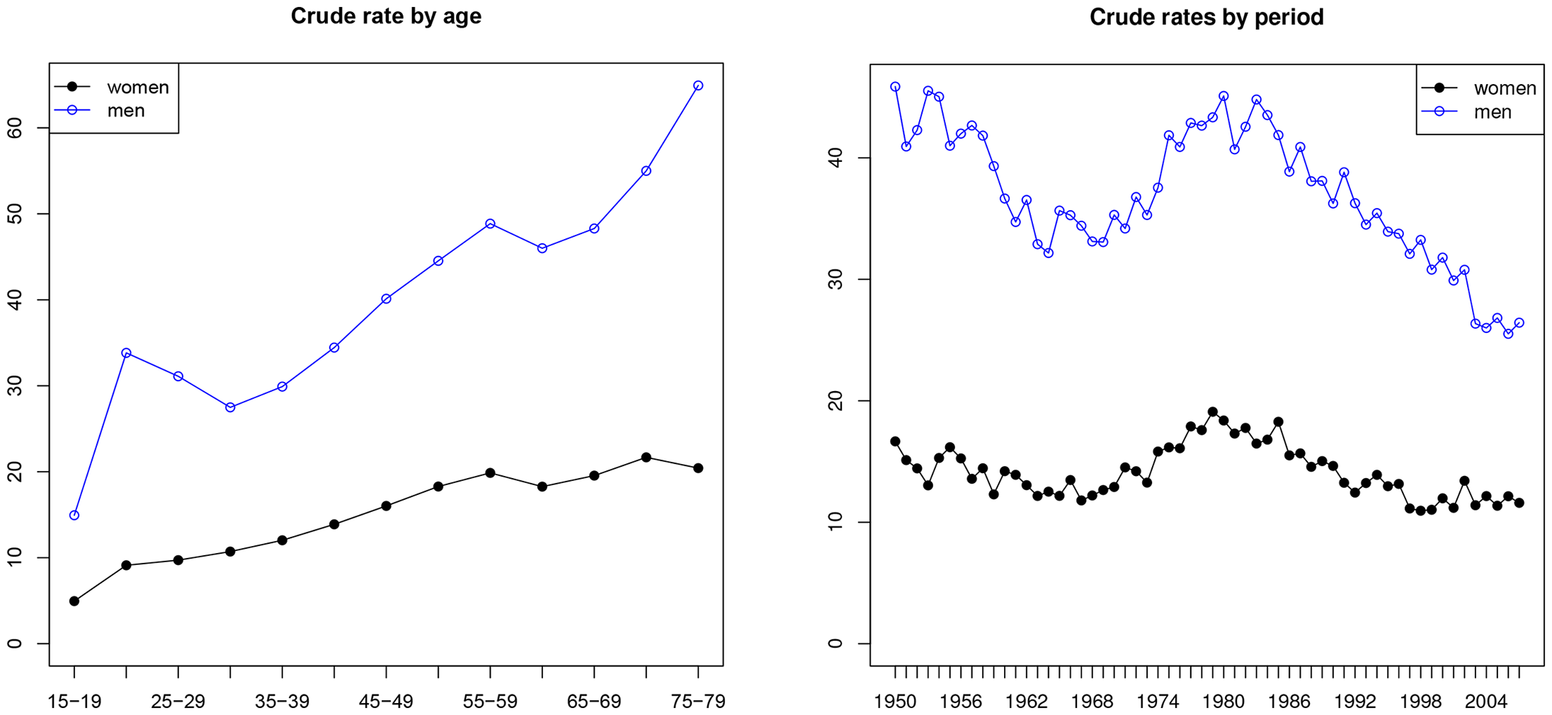
Crude rates per 100,000.

Following Riebler et al. (2012), we will replace the period effect with a family integration index composed from marriage and divorce rates as shown in Section ‘Empirical illustration’. This choice is motivated by Durkheim’s theory from the late 1800s and numerous subsequent work considering the relationship between marital status and suicide.

Figure 2.

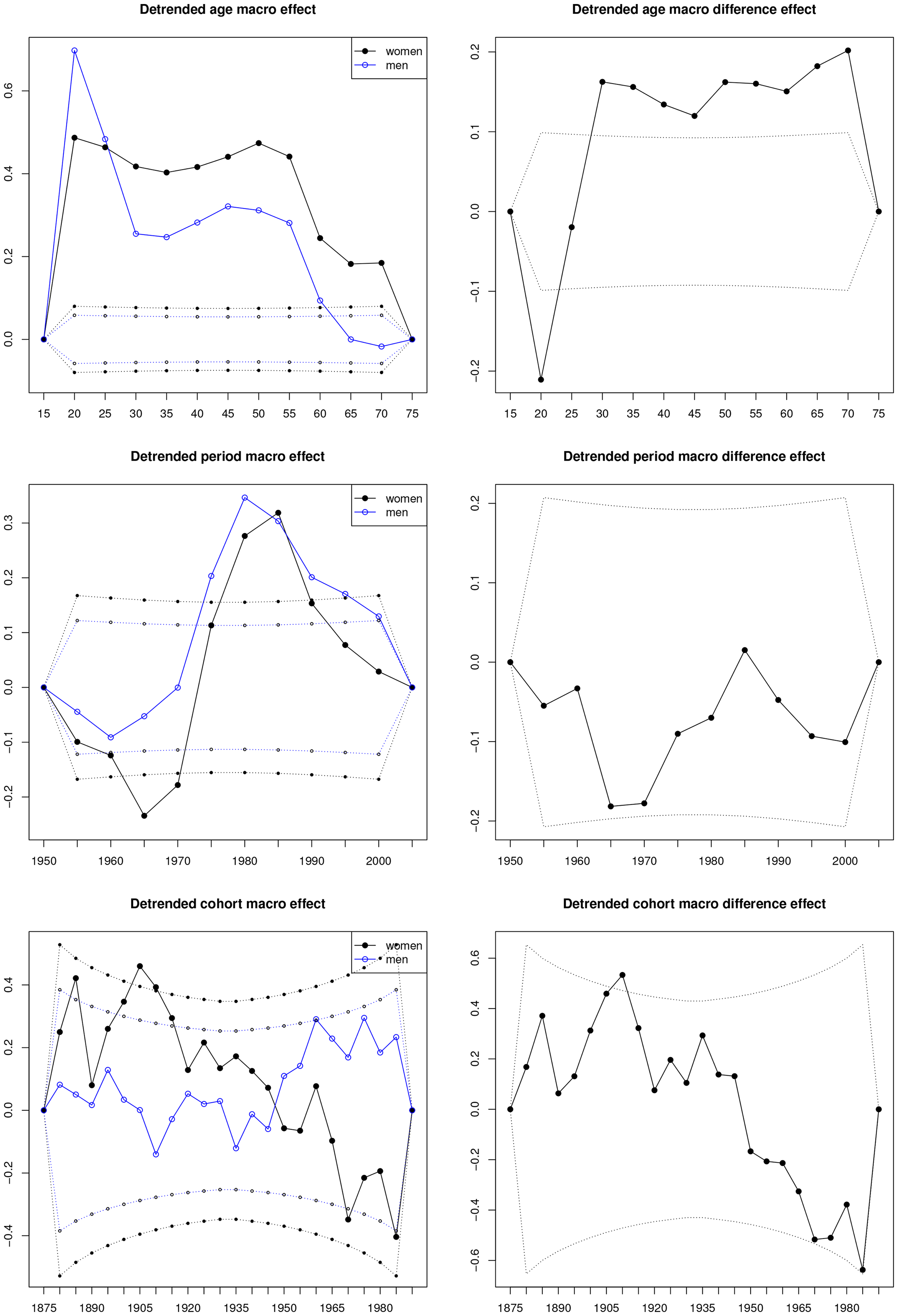
Detrended macro effects. Solid lines are estimates and dotted lines are $\pm 2$ standard errors centred at zero. On the left, macro effects are shown for women (bullets) and men (circles). On the right, cross-sample difference are shown. Detrending is done so that all graphs start and end in zero.

Figure 3.

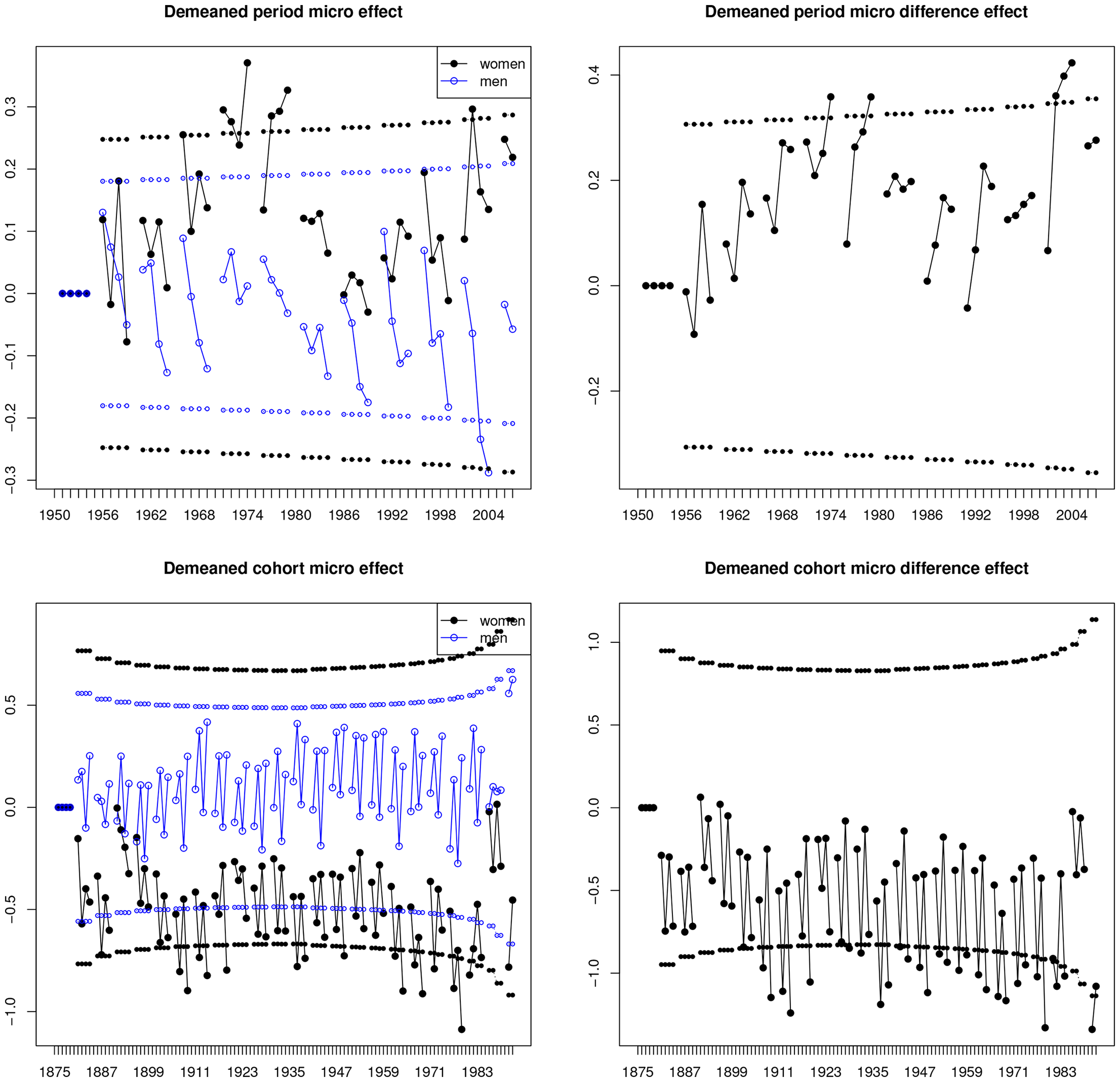
Demeaned micro effects. Solid lines are estimates and small plot symbols are $\pm 2$ standard error centred at zero. The micro effects are measured relative to the macro effects and are therefore shown in groups of 4. On the left, micro effects are shown women (bullets) and men (circles). On the right, cross-sample differences are shown. Demeaning is done by restricting initial levels to zero for all 4 micro frequencies.

Figure 4.

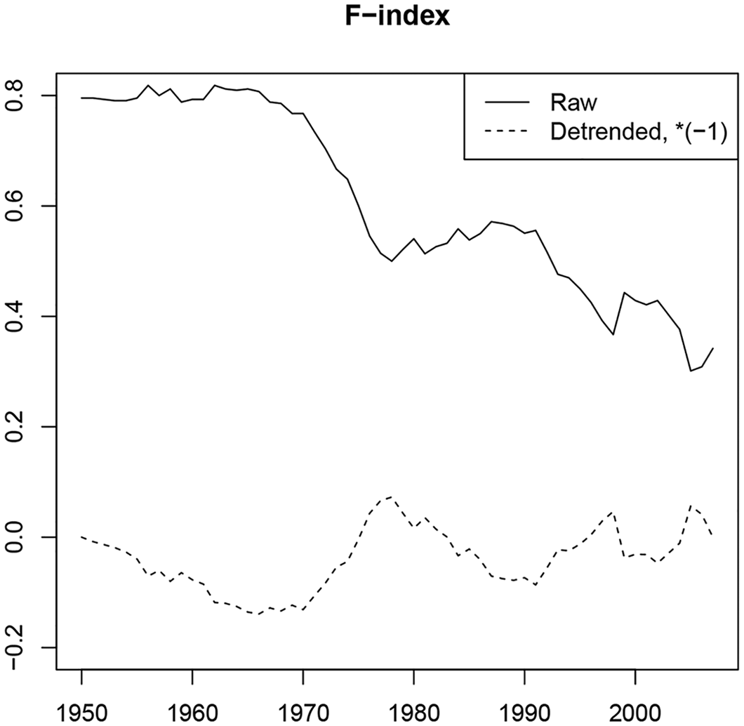
F-index. The solid line shows the raw F-index. The dashed line, the F-index is detrended to start and end in zero. It is also multiplied by -1 to facilitate comparison with the detrended cross-sample difference of the macro period effect in Figure 2.

Riebler et al. (2012) applied a Bayesian, two-sample, age-period-cohort, over-dispersed Poisson model. They found a common period effect for the two samples and investigated the extent to which the period effects could be replaced by socio-economic time series.

A theory for two-sample age-period-cohort analysis follows. Subsequently, we reanalyze the data in Section ‘Empirical illustration’ by implementing this theory in a generalized linear model. Comments on Bayesian analysis are given in Appendix A.4 in the online Supplemental Material.

The Two-sample Model for Regular Data

Suppose we have two samples of data in the form of rates, counts, or doses and responses. The samples are organized in terms of common regular age-period arrays. We first review the organization of the data. Then, we introduce the unrestricted age-period-cohort model and the age-period-cohort problem, which we address through a reparametrization in terms of invariant parameters. Finally, we turn to a discussion of relevant hypotheses. A generalization to mixed-frequency age-period arrays follows in Section ‘The Two-sample Model for Mixed Data’.

Data Structure

We consider two data arrays with the same regular structure with $A$ age levels and $P$ period levels. Throughout this section, the increments in age and in period have the same length. In practice, increments are often yearly. This results in the index set

$${\mathcal{I}}_{age,per}=\{1\le age\le A\text{a}nd1\le \mathit{p}\mathit{e}\mathit{r}\le \mathit{P}\}\mathit{.}$$

(1)

Cohorts are defined according to the cohort identity

$$coh=per+A-age.$$

(2)

The possible cohorts over the set ${\mathcal{I}}_{age,per}$ are

$${\mathcal{I}}_{coh}=(1,\dots ,C),\text{w}here\mathit{C}\mathit{=}\mathit{A}\mathit{+}\mathit{P}\mathit{-}1\mathit{.}$$

(3)

The Two-sample Age-period-cohort Model

The two-sample age-period-cohort model has the well-known age-period-cohort problem, which we present. We circumvent this problem by finding invariant parameters and reparametrizing the model in terms of those invariant parameters. One could say that the initial formulation of the model is a wish list of effects we may want to include, while the reparametrized model describes the consequences of these wishes in a way that is better suited for statistical analysis.

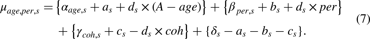
Age-period-cohort model formulated with level effects

We set up age-period-cohort models for each of the two samples. This is a model for the predictor, which could be the expected outcome in a linear model or the log expected outcome in a log-linear model. It has the form

$$\begin{array}{r}{\mu }_{age,per,s}={\alpha }_{age,s}+{\beta }_{per,s}+{\gamma }_{coh,s}+{\delta }_s\text{f}or\mathit{a}\mathit{g}\mathit{e}\mathit{,}\mathit{p}\mathit{e}\mathit{r}\in {\mathcal{I}}_{\mathit{a}\mathit{g}\mathit{e}\mathit{,}\mathit{p}\mathit{e}\mathit{r}}\mathit{\text{ and }}\mathit{s}\mathit{=}\mathit{1}\mathit{,}\mathit{2}\mathit{,}\end{array}$$

(4)

where ${\alpha }_{age,s}$ is the age effect at a given $age$ in sample $s$ , where ${\beta }_{per,s}$ and ${\gamma }_{coh,s}$ are the sample specific period and cohort effects, and where ${\delta }_s$ is the sample specific intercept.

The time effects on the right hand side of the model equation (4) have dimension

$$q=2(A+P+C+1)=4(A+P),$$

(5)

as each sample $s$ has $A$ ages, $P$ periods, $C=A+P-1$ cohorts and 1 intercept.

The age-period-cohort problem

We describe the classicial age-period-cohort problem and how this effects the two-sample model. In short, the problem is that the time effects on the right hand side of (4) are not identified from the possible variation of the left hand side of (4).

It is well-understood that the age-period-cohort problem arises, since the cohort identity (2) implies the identity

$$0=\{a_s+d_s\times (A-age)\}+\{b_s+d_s\times per\}+\{c_s-d_s\times coh\}-\{a_s+b_s+c_s\},$$

(6)

for any scalars $a_s$ , $b_s$ , $c_s$ , $d_s$ . We see that, for instance, the scalars $a_s$ cancel when combining the first and the last curly bracket terms. Similarly, the slopes $d_s$ cancel due to the cohort identity (2). Now, adding the identity (6) to the predictor (4) gives

$$\begin{array}{rl}{\mu }_{age,per,s}=& \{{\alpha }_{age,s}+a_s+d_s\times (A-age)\}+\{{\beta }_{per,s}+b_s+d_s\times per\}\\ & +\{{\gamma }_{coh,s}+c_s-d_s\times coh\}+\{{\delta }_s-a_s-b_s-c_s\}.\end{array}$$

(7)

The identity (7) shows how we can transform the time effects on the right hand side by adding linear terms without changing the predictor on the left hand side. As the predictor ${\mu }_{age,per,s}$ appearing on the left hand side of (7) does not change with $a_s,b_s,c_s,d_s$ , we say that it is invariant to the transformations of the time effects appearing on the right hand side of (7). The transformations in (7) describe the identification problem completely as stated by Carstensen (2007) and proved in Kuang et al. (2008).

There are $2\times 4=8$ possible values of $a_s,b_s,c_s,d_s$ for $s=1,2$ . Subtracting 8 from the time effect dimension $q$ defined in (5) shows that the dimension of the variation of the predictor is

$$p=q-2\times 4=2\times (2A+2P-4).$$

(8)

We will proceed by finding a $p$ -dimensional parameter that is invariant to the manipulations in (7) and that fully describes the predictor variation.

Invariant parameters

We address the age-period-cohort problem by working with invariant parameters. These are parameters that do not change with the transformations in (7). The idea of the approach is to generalize the notion of contrasts in two-way analysis. Contrasts eliminate unidentified common levels by taking differences. In the age-period-cohort context, we eliminate unidentified common slopes by taking double differences. In accordance with statistical theory, the resulting parameters are said to be invariant to the transformations (7) (Cox and Hinkley 1974).

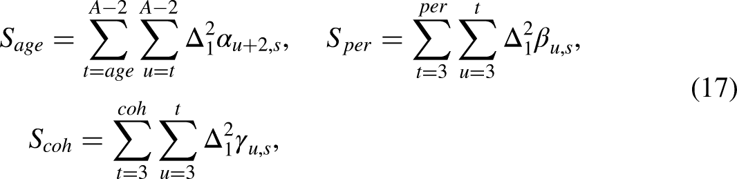
We decompose the period effects ${\beta }_{per,s}$ into two parts: The non-linear and the linear components. We express the non-linear components of ${\beta }_{per,s}$ in terms of double differences and show that these are invariant. Next, we combine the linear components from all time effects to form an invariant linear plane.

Invariant non-linear components: We define the double differences of the period effects ${\beta }_{per,s}$ as follows. Let ${\mathrm{\Delta }}_1$ be the 1-period difference operator, so that ${\mathrm{\Delta }}_1{\beta }_{per,s}={\beta }_{per,s}-{\beta }_{per-1,s}$ . Applied twice, we get second differences

$${\mathrm{\Delta }}_1^2{\beta }_{per,s}={\mathrm{\Delta }}_1{\beta }_{per,s}-{\mathrm{\Delta }}_1{\beta }_{per-1,s}={\beta }_{per,s}-2{\beta }_{per-1,s}+{\beta }_{per-2,s}.$$

(9)

The double differences ${\mathrm{\Delta }}_1^2{\beta }_{per,s}$ are invariant to the transformations in (7). Indeed, ${\beta }_{per,s}$ and its linear transformation ${\beta }_{per,s}+b_s+d_s\times per$ have the same double differences, since ${\mathrm{\Delta }}_1^2(b_s+d_s\times per)={\mathrm{\Delta }}_1(d_s)=0$ . Moreover, the double differences can be expressed in terms of double differences of the predictor (Fienberg and Mason 1979; Martínez Miranda et al. 2015). For instance,

$${\mathrm{\Delta }}_1^2{\beta }_{per,s}={\mu }_{age,per,s}-{\mu }_{age,per-1,s}-{\mu }_{age-1,per-1,s}+{\mu }_{age-1,per-2,s}.$$

(10)

The double differences are often quite natural objects to study. For instance, in a logistic model they correspond to log-odds ratios.

The consequence of the invariance is that we can learn about the double differences without any worry about the age-period-cohort problem. Moreover, if two researchers choose different ad hoc identification schemes, such as setting different choices of four time effect values to zero, but otherwise use the same estimation method, then these researchers will get the same fit and their estimates of the second diffences ${\mathrm{\Delta }}_1^2{\beta }_{per,s}$ will be identical due to equation (10).

In a similar fashion, the age and cohort double differences ${\mathrm{\Delta }}_1^2{\alpha }_{age,s}$ and ${\mathrm{\Delta }}_1^2{\gamma }_{coh,s}$ are invariant to the transformations in (7). The full set of invariant double differences is

$$\begin{array}{rl}& {\mathrm{\Delta }}_1^2{\alpha }_{age,s},{\mathrm{\Delta }}_1^2{\beta }_{per,s},{\mathrm{\Delta }}_1^2{\gamma }_{coh,s}\\ & \text{f}or3\le \mathit{a}\mathit{g}\mathit{e}\le \mathit{A}\mathit{,}3\le \mathit{p}\mathit{e}\mathit{r}\le \mathit{P}\mathit{,}3\le \mathit{c}\mathit{o}\mathit{h}\le \mathit{C}\mathit{.}\end{array}$$

(11)

The dimension of this set of double differences is $2\times (2A+2P-7)$ coming from $A-2$ ages, $P-2$ periods and $C-2=A+P-3$ cohorts. We note that this dimension is $2\times 3=6$ less than $p=2\times (2A+2P-4)$ , see (8).

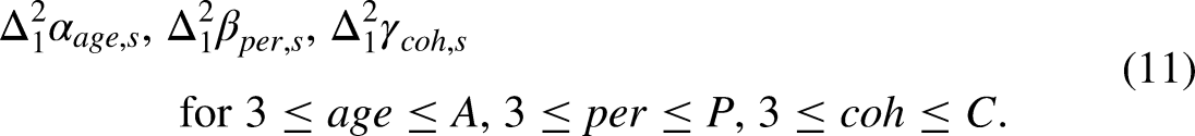
The points sofar have been made in the literature at least as far back as (Fienberg and Mason 1979). Now, we will deviate from the classic literature. The aim is to express the predictor in terms of invariant parameters. This will allow us to conduct the entire analysis in terms of invariant parameters without worrying about the original time effect parametrization (4) and its identification problem. This requires further 3 invariant parameters for each sample as proposed by Kuang et al. (2008).

Invariant linear components. When taking double differences of the period effects ${\beta }_{per,s}$ , we loose information about the level and the linear slope. Somehow, these lost effects must be included in an invariant fashion in order to get back to the predictor. We will express the lost level as ${\beta }_{per,1}$ and the lost slope as the first difference $\mathrm{\Delta }{\beta }_{per,2}={\beta }_{per,2}-{\beta }_{per,1}$ . The trick is to combine these unidentified effects to achieve identified and invariant parameters. Since, this is all about combining levels and slope, it is to be expected that we can find invariant linear planes.

Linear planes can be defined from a level and two slopes. The level is chosen from

$${\mu }_{A,1,s}={\alpha }_{A,s}+{\beta }_{1,s}+{\gamma }_{1,s}+{\delta }_s,$$

(12)

where levels of the time effects add up to a particular value of the predictor. Hence, this combination is invariant as adding $a_s$ to ${\alpha }_{A,s}$ , $b_s$ to ${\beta }_{1,s}$ , $c_s$ to ${\gamma }_{1,s}$ while subtracting their sum from ${\delta }_s$ leaves the predictor in (12) unchanged.

The slopes are chosen as an age-cohort slope and a period-cohort slope given by

$${\lambda }_s={\mu }_{A-1,1,s}-{\mu }_{A,1,s}={\mathrm{\Delta }}_1{\gamma }_{2,s}-{\mathrm{\Delta }}_1{\alpha }_{A,s}$$

(13)

$${\nu }_s={\mu }_{A,2,s}-{\mu }_{A,1,s}={\mathrm{\Delta }}_1{\gamma }_{2,s}+{\mathrm{\Delta }}_1{\beta }_{2,s},$$

(14)

Both slopes are invariant. Indeed, for the former, ${\mathrm{\Delta }}_1\{{\alpha }_{age,s}+a_s+d_s\times (A-age)\}={\mathrm{\Delta }}_1{\alpha }_{age,s}-d_s$ and ${\mathrm{\Delta }}_1({\gamma }_{coh,s}+c_s-d_s\times coh)={\mathrm{\Delta }}_1{\gamma }_{coh,s}-d_s$ with $d_s$ canceling when taking the difference.

The slopes in (13)–(14) cannot be separated into individual slopes for age, period, cohort. By imposing additional constraints such as ${\mathrm{\Delta }}_1{\beta }_{2,s}=0$ , we get a unique value for ${\mathrm{\Delta }}_1{\gamma }_{2,s}={\lambda }_s$ from (14). It is common to refer to this uniqueness as identification. However, this choice is not invariant as it is observationally equivalent to ${\mathrm{\Delta }}_1{\beta }_{2,s}=b_s$ and ${\mathrm{\Delta }}_1{\gamma }_{2,s}={\lambda }_s-b_s$ for any $b_s$ .

Full set of invariant components. We combine the double differences, levels and slopes in a vector $\xi =({\xi }_1^{\prime },{\xi }_2^{\prime }{)}^{\prime }$ , where

$$\begin{array}{rl}{\xi }_s=& ({\mu }_{A,1,s};{\lambda }_s;{\nu }_s;{\mathrm{\Delta }}_1^2{\alpha }_{age,s}\text{ for }3\le \mathit{a}\mathit{g}\mathit{e}\le \mathit{A}\mathit{;}\\ & {\mathrm{\Delta }}_1^2{\beta }_{per,s}\text{ for }3\le \mathit{p}\mathit{e}\mathit{r}\le \mathit{P}\mathit{;}{\mathit{\Delta }}_{\mathit{1}}^{\mathit{2}}{\gamma }_{\mathit{c}\mathit{o}\mathit{h}\mathit{,}\mathit{s}}\mathit{\text{ for }}\mathit{3}\le \mathit{c}\mathit{o}\mathit{h}\le \mathit{C}{)}^{\prime }\mathit{.}\end{array}$$

(15)

The parameter $\xi$ has dimension $p$ as given in (8). This is therefore an invariant parameter that has the right dimension.

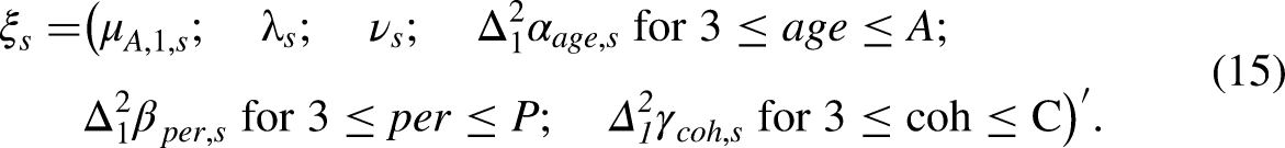
Writing the predictor in terms of invariant parameters

We write the predictor as a function of the invariant parameter in order to reparametrize the model. The main purpose of this step is to facilitate computer code. That is, we can sidestep the initial formulation of the model in (4) and the age-period-cohort problem (7), and just think of age-period-cohort modeling in terms of a standard regression model. For the practitioner, who relies on the code of someone else, the main consequence of the following argument is that hypotheses can be thought of in terms of the invariant parameter (15).

Representation of predictor. We have the one-sample representation

$$\begin{array}{rl}{\mu }_{age,per,s}& ={\mu }_{A,1,s}+(A-age){\lambda }_s+(per-1){\nu }_s\\ & +S_{age,s}+S_{per,s}+S_{coh,s},\end{array}$$

(16)

from Martínez Miranda et al. (2015). The first three terms of the representation define a linear plane, where ${\lambda }_s$ is the age-cohort slope and ${\nu }_s$ is the period-cohort slope. The $S$ terms are the non-linear time effects. They have expressions

$$S_{age}=\sum _{t=age}^{A-2}\sum _{u=t}^{A-2}{\mathrm{\Delta }}_1^2{\alpha }_{u+2,s},S_{per}=\sum _{t=3}^{per}\sum _{u=3}^t{\mathrm{\Delta }}_1^2{\beta }_{u,s},S_{coh}=\sum _{t=3}^{coh}\sum _{u=3}^t{\mathrm{\Delta }}_1^2{\gamma }_{u,s},$$

(17)

with the convention that empty sums are zero. These terms represent the original time effects, each with two zero constraints. Plots of these double sums are typically trending and not offering an appealing interpretation. A more useful interpretation follows in the empirical application, but see also Chauvel and Schröder 2014. The levels and linear slopes in (16) combine to describe a linear plane.

Design matrix. When formulating the regression in statistical software, we will need to write down a design matrix. The representation (16) is a linear function of the canonical parameter $\xi$ , but the exact expression is not so obvious because of the double sums. A further manipulation in Appendix A.1 in the online Supplemental Material expresses the predictor as a linear function of a design vector $x_{age,per}$ which is common accross samples and with coefficients given by invariant parameters. That is,

$${\mu }_{age,per,s}={\xi }_1^{\prime }{x}_{age,per}{1}_{(s=1)}+{\xi }_2^{\prime }{x}_{age,per}{1}_{(s=2)}.$$

(18)

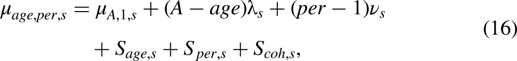
The exact expression of the design vector $x_{age,per}$ is needed for two purposes. First, when seeking to estimate the age-period-cohort model using a statistical package one will regress outcomes $y_{age,per}$ on the design vector, typically through a linear model or a generalized linear model. Second, once an estimate of the invariant parameter $\xi$ is available, one will be interested in computing and plotting the predictor and its consituents, the double sums of double differences and the linear plane. This is all done in the apc package for R (Nielsen 2015).

Invariance and identification conditions. The equations (16), (18) parametrize the age-period-cohort predictor in terms of the invariant parameter. As the aim is to use this for estimation, we must be assured that the information content is the same as with the original expression for the predictor in terms of the time effects. Thus we need to know that

$(a)$ $\xi$ is a linear function of $\mu$ that is invariant to the transformations in (7);

$(b)$ $\mu$ is a linear function of $\xi$ given by (16);

$(c)$ The parameter $\xi$ is exactly identified in that ${\xi }^{†}\ne {\xi }^{\text{‡}}$ implies $\mu ({\xi }^{†})\ne \mu ({\xi }^{\text{‡}})$ .

In other words, in the original model (4), the time effects generate a certain variation in the predictor, which we will match with the variation in the data. The age-period-cohort problem means that different time effects can generate the same predictor. This redundancy is eliminated when parametrizing the predictor in terms of the canonical parameter. Since $\xi$ is invariant and identifies $\mu$ , we can work freely with $\xi$ just as we work with the parameters in standard regression models: We can brush the age-period-cohort problem aside, we can interpret parameters freely, and we can trust standard degrees of freedom calculations when testing hypotheses.

The property that the predictor ${\mu }_{age,per,s}$ is a linear function of an identified, freely varying parameter $\xi$ is a coveted property in statistical theory. In practice, we will typically embed the predictor in a generalized linear model. In the context of exponential family theory or more broadly generalized linear models, $\xi$ will be the canonical parameter and we will refer to it as such (Sundberg 2019).

We must check that $(a)$ – $(c)$ are satisfied. $(a)$ holds since $\xi$ is a function of $\mu$ that is invariant. Indeed, the period double differences are expressed in terms of $\mu$ in (10) and it is argued just before that the period double differences are invariant. Similar results apply for the age and cohort double differences. $(b)$ holds since $\mu$ can be expressed in terms of $\xi$ as done in (16). $(c)$ is checked in Kuang et al. (2008).

Restrictions on the Age-period-cohort Parameters

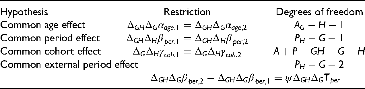
In the context of the two-sample model it is natural to ask if any of the age, period or cohort effects are common? Initially, we consider the hypotheses of common period effects and whether period effects could be driven by some external developments in the wider society. Finally, we consider a wider range of age, period, cohort hypotheses.

The hypothesis of common period double differences

In a two-sample analysis, it will often be relevant to ask if the period effects could be common across the two samples. We need to be careful when posing this question. The non-linear parts of the period are identified whereas the linear parts are not. Thus, restrictions on the restrictions on the non-linear parts will be binding, whereas restrictions on the linear parts are not binding.

The hypothesis that the non-linear parts of the period effects are common is that

$${\mathrm{\Delta }}_1^2{\beta }_{per,1}={\mathrm{\Delta }}_1^2{\beta }_{per,2}\text{f}or3\le per\le P.$$

(19)

The degrees of freedom of the hypothesis is $P-2$ . The interpretation of this hypothesis follows from the representation (16). We see that the double sum of double differenced period effects will be common while there are no constraints to the linear planes.

For estimation under the hypothesis it is convenient to rewrite the design vector expression for the predictor in (18). By adding and subtracting ${\xi }_1^{\prime }{x}_{age,per}{1}_{(s=2)}/2$ and ${\xi }_2^{\prime }{x}_{age,per}{1}_{(s=1)}/2$ we get

$${\mu }_{age,per,s}=(\frac{{\xi }_1+{\xi }_2}{2}{)}^{\prime }{x}_{age,per}+(\frac{{\xi }_1-{\xi }_2}{2}{)}^{\prime }{x}_{age,per}\{1_{(s=1)}-1_{(s=2)}\}.$$

(20)

Thus, restricting the period double differences to be common is equivalent to a zero restriction on the second parameter $({\xi }_1-{\xi }_2)/2$ with $P-2$ degrees of freedom.

The hypothesis of common period effects

A hypothesis formulated directly on the common period effects may appear attractive. Yet, it turns out to be observationally equivalent to the hypothesis of common period double differences in (19). The hypothesis of common period effects is

$${\beta }_{per,1}={\beta }_{per,2}\text{f}or1\le per\le P.$$

(21)

This formulation implies the $P-2$ restrictions for the double differences in (19) as well as one level constraint, ${\beta }_{1,1}={\beta }_{1,2}$ , and one slope constraint, $\mathrm{\Delta }{\beta }_{2,1}=\mathrm{\Delta }{\beta }_{2,2}$ . Can we learn something from these two additional constraints? The answer is negative and the explanation goes to the heart of the age-period-cohort problem. Due to the identity (6), the constraints $\mathrm{\Delta }{\beta }_{2,1}=\mathrm{\Delta }{\beta }_{2,2}+b$ are observationally equivalent for any scalar $b$ .

If it were true that the linear, cross-sample differenced, period effects were zero, then one would be able to identify the cross-sample age and cohort slopes as argued by Riebler and Held (2010). However, this truism remains untestable, as the linear parts of an age-cohort model and of an age-period-cohort model remain observationally equivalent. For further details, see Appendix A.2 in the online Supplemental Material.

The point that the linear parts of age-period-cohort models are observationally equivalent to the linear parts of age-cohort models has been made in various places in the literature. An early reference is Clayton and Schifflers (1987). Nielsen and Nielsen (2014) described this in terms of linear algebra. Keiding and Andersen (2016) raised the point in a comment on a paper concerned with the question whether delaying childbearing to older ages might be associated with more positive educational and health outcomes for the children. Fannon and Nielsen (2019) give a detailed analysis of the model where only linear planes are present.

To conclude, from a statistical viewpoint, the hypothesis (19) of common double-differenced period effects, ${\mathrm{\Delta }}^2{\beta }_{per,1}={\mathrm{\Delta }}^2{\beta }_{per,2}$ is observationally equivalent to the hypothesis (21) of common period effects ${\beta }_{per,1}={\beta }_{per,2}$ . Thus, we can only learn about non-linear terms. Working with the canonical parameters clarifies which questions we can and cannot ask. Therefore it removes risks of confusion over degrees of freedom and confusion over the identification status of time effects. Working with the time effects will at best give the same analysis, and a worst add arbitrariness to the analysis.

Replacing period effect with time series

Could it be that socio-economic effects explain the period movements that we see in the data? In other words, does the period effect follow some external time series? Hypotheses of this kind can be tested, but we need to take the age-period-cohort problem into account. The period effect is only determined up to arbitrary linear trends, see (6). Thus, the testable hypothesis is that the non-linear part of the period effect follows the non-linear part of the external time-series.

The hypothesis can be implemented by replacing the double differenced period parameter ${\mathrm{\Delta }}_1^2{\beta }_{per}$ by the double differences of the external time series multiplied by a free scalar parameter, that is $\psi {\mathrm{\Delta }}_1^2{T}_{per}$ say. The degrees of freedom will then be the number of period double differences, $P-2$ , minus one due to the free parameter $\psi$ .

In a two-sample age-period-cohort model the external time series restriction can be done in various ways. It can be imposed on the cross-sample differenced parameter ${\xi }_1-{\xi }_2$ , or on the common parameter ${\xi }_1+{\xi }_2$ , or on the individual parameters ${\xi }_1$ , ${\xi }_2$ .

Further sub-models

Other sub-models may be relevant. We give an overview, but see also Fannon and Nielsen 2019. We will be particularly interested in restrictions on the cross-sample differenced predictor $({\xi }_1-{\xi }_2)/2$ , while leaving the common parameter $({\xi }_1+{\xi }_2)/2$ unrestricted.

A period-cohort model for the cross-sample differenced predictors arises when the non-linear parts of the age effects are common, that is ${\mathrm{\Delta }}_1^2{\alpha }_{age,1}={\mathrm{\Delta }}_1^2{\alpha }_{age,2}$ . The degrees of freedom of the hypothesis is $A-2$ .

An age-period model for the cross-sample differenced predictors arises with the restriction ${\mathrm{\Delta }}_1^2{\gamma }_{coh,1}={\mathrm{\Delta }}_1^2{\gamma }_{coh,2}$ . The degrees of freedom of the hypothesis is $C-2$ .

An age-drift model arises when both the period and cohort cross-sample double differences are restricted to be zero. That is ${\mathrm{\Delta }}_1^2{\beta }_{per,1}={\mathrm{\Delta }}_1^2{\beta }_{per,2}$ and ${\mathrm{\Delta }}_1^2{\gamma }_{coh,1}={\mathrm{\Delta }}_1^2{\gamma }_{coh,2}$ . The degrees of freedom is the count of parameters $P+C-4$ . This hypothesis does not restrict the linear plane. For further discussion, see Clayton and Schifflers 1987.

A pure age model occurs when restricting the age-drift model further by requiring a zero cross-sample period-cohort slope through ${\nu }_1={\nu }_2$ . This gives one further constraint.

A constant model occurs when only the cross-sample level ${\delta }_1-{\delta }_2$ is allowed to vary freely. This gives further $A-2$ constraints compared to the age cross-sample model.

The zero model has ${\xi }_1={\xi }_2$ so that ${\mu }_{age,per,1}-{\mu }_{age,per,2}=0$ . There are no degrees of freedom left. We can add the identity (6) to ${\mu }_{age,per,1}-{\mu }_{age,per,2}=0$ showing that there is no scope for identifying the linear parts of the time effects. This point was made in the comment by Keiding and Andersen (2016) on an empirical analysis linking maternal age and offspring outcomes.

The Two-sample Model for Mixed Data

The two-sample age-period-cohort model is generalized to general mixed-frequency arrays building on Nielsen (2022), henceforth N22. We proceed as before by reviewing the organization of the data, introducing the unrestricted age-period-cohort model, analyzing the identification problem and giving an invariant, identified reparametrization.

Data Structure

Mixed frequency age-period data arise by a fairly easy generalization of the regular data we have seen before. However, it is now more complicated to describe which cohort values are possible.

The general mixed-frequency setup has $A_G$ age groups of length $G$ covering $A=A_{G}G$ ages and $P_H$ period groups of length $H$ covering $P=P_{H}H$ periods. We assume that the largest common divisor of $G$ and $H$ is unity. If groups have common divisor larger than unity, such as 10 and 4, we can scale by the common divisor of 2. The Swiss data has $G=5$ and $H=1$ . Table 1 shows a situation with $G=5$ and $H=3$ .

Table 1.

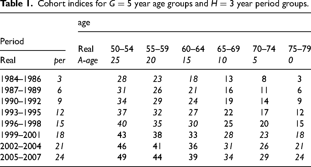
Cohort indices for $G=5$ year age groups and $H=3$ year period groups.

		age
Period		Real	50–54	55–59	60–64	65–69	70–74	75–79
Real	$per$	$A$ - $age$	25	20	15	10	5	0
1984–1986	3		28	23	18	13	8	3
1987–1989	6		31	26	21	16	11	6
1990–1992	9		34	29	24	19	14	9
1993–1995	12		37	32	27	22	17	12
1996–1998	15		40	35	30	25	20	15
1999–2001	18		43	38	33	28	23	18
2002–2004	21		46	41	36	31	26	21
2005–2007	24		49	44	39	34	29	24

An age-period data array has index set

$${\mathcal{I}}_{age,per}:\{\begin{array}{cc}age=A-gG& \text{w}hereg=0,1,\dots ,A_G-1,\\ per=H+hH& \text{w}hereh=0,1,\dots ,P_H-1.\end{array}$$

(22)

With $coh=per+A-age$ as in (2), we get $coh=H+hH+gG$ , so that the smallest and largests cohort are $H$ and $C=A+P-G$ . We give three examples.

Regular data arise when $G=H=1$ . In that case $A=A_G$ and $P=P_H$ and we arrive at the index set (1) given above.

The Swiss data has $G=5$ but $H=1$ . It has $A_G=13$ age groups giving $A=A_{G}G=65$ ages, while there are $P=58$ periods. The largest cohort is $C=A+P-G=118$ .

Mixed frequency data with $G\ne H$ have a more complicated cohort structure than the Swiss data. Table 1 illustrates the possible cohorts for a case with $G=5$ and $H=3$ . There are $A_G=6$ age groups and $P_H=8$ period groups spanning $A=A_{G}G=30$ ages and $P=P_{H}H=24$ periods. The smallest and largest cohorts are $H=3$ and $C=49$ . Certain cohort values are skipped as noted by Holford (2006). The skipped cohort values are $4,5,7,10$ and $42,45,47,48$ . This corresponds to $H=3$ plus the values $1,2,4,7$ and $C=49$ minus the same values. Table 1 also indicates macro blocks of dimension $GH=15$ with italic and roman fonts. Note that top left and bottom right macro blocks are identical apart from trimming.

The fact that some cohort values are skipped will be rather important for understanding how many parameters the an age-period-cohort model has. In turn this will feed into the calculation of degrees of freedom. It turns out that there is theory for the skipping (N22). The possible cohorts over the set ${\mathcal{I}}_{age,per}$ are of the form

$${\mathcal{I}}_{coh}=(H,\dots ,C)\mathrm{\setminus }(H+c,C-c:c\in {\mathcal{N}}_{G,H}).$$

(23)

Thus, the cohorts take values between $H$ and $C$ apart from some skipped values at either end that are represented by a set ${\mathcal{N}}_{G,H}$ . The count of elements in ${\mathcal{N}}_{G,H}$ is denoted $S_{G,H}$ .

The skipping is akin to the coin problem in algebra : If we have groups (coins) of denomination $G$ , $H$ , which cohorts (monetary amounts) can we form? To answer this question, we note the previously stated assumption that $G,H$ have no common divisor larger than unity. Then, the skipping problem arises when $G,H\ge 2$ . Let ${\mathcal{N}}_{G,H}$ denote the non-representable cohorts (monetary amounts). The Frobenius number $F_{G,H}=GH-G-H$ is the largest non-representable number, while Sylvester pointed out that the number of non-representable numbers is $S_{G,H}=(G-1)(H-1)/2$ (Ramírez Alfonsín 2005). Algorithms for finding ${\mathcal{N}}_{G,H}$ are discussed in N22. In general, the number of possible cohorts is then $C-(H-1)-2S_{G,H}$ , which equals $A+P-GH$ .

In the example with $G=5$ , and $H=3$ there are $S_{G,H}=4$ non-representable numbers in ${\mathcal{N}}_{5,3}$ with largest value $F_{G,H}=7$ . With $A=30$ and $P=24$ then $C=49$ , but only $A+P-GH=39$ cohorts will be present in the sample, since we skip 8 values and the 2 values less than $H=3$ are not possible.

The Two-sample Age-period-cohort Model

We now present the two-sample age-period-cohort model for mixed frequency data. The approach is the same as for the regular case. We will need to discuss how the age-period-cohort problem changes. Based on that, invariant parameters can be found and the predictor will have to represented in terms of those.

Age-period-cohort model formulated with level effects

We consider exactly the same two-sample age-period-cohort model as before for the mixed frequency data. This gives the same model equation as in (4), that is

$$\begin{array}{r}{\mu }_{age,per,s}={\alpha }_{age,s}+{\beta }_{per,s}+{\gamma }_{coh,s}+{\delta }_s\text{f}orage,per\in {\mathcal{I}}_{age,per}\text{a}nds=1,2.\end{array}$$

(24)

The time effects on the right hand side of the model equation have dimension

$$q=2(A_G+P_H+A+P-GH+1),$$

(25)

as each sample has $A_G$ ages, $P_H$ periods, $A+P-GH$ cohorts and 1 intercept. This calculation accounts for the skipping.

The age-period-cohort problem

We are now faced with new identification issues. First, we have the standard age-period-cohort problem that only one level and two linear slopes are identifiable. Second, the mixed-frequency indexation results in additional constraints as noted by Fienberg and Mason (1979). N22 describes the full set of constraints for one mixed-frequency sample. This carries immediately over to the two-sample model.

The mixed-frequency structure results in macro steps of length $GH$ in both the age and the period dimension. At the macro level we will have the usual age-period-cohort problem of manipulation with arbitrary linear trends.

In addition, we get a micro effect in age by adding $G$ to each of the age macro steps. We can also add $G$ to the cohort macro steps, but not to the period macro steps as period moves in multiples of $H$ . Thus, the age micro effects are linked with the cohorts but not with the periods. We can express this more precisely as follows. Recall that two integers $i,j$ are congruent modulo $G$ , if $G$ divides their difference $i-j$ and we write $i\equiv j\mathrm{mod}G$ . For instance, $5\equiv 8\mathrm{mod}3$ . Combining the assumption that $G$ divides $age$ and $A$ with the relation $coh=per+A-age$ from (2) gives the congruence $coh\equiv per\mathrm{mod}G$ . In a similar fashion, $coh\equiv A-age\mathrm{mod}H$ .

Combining the possible macro and micro transformations gives the following mixed-frequency, one-sample identity, which generalizes (6),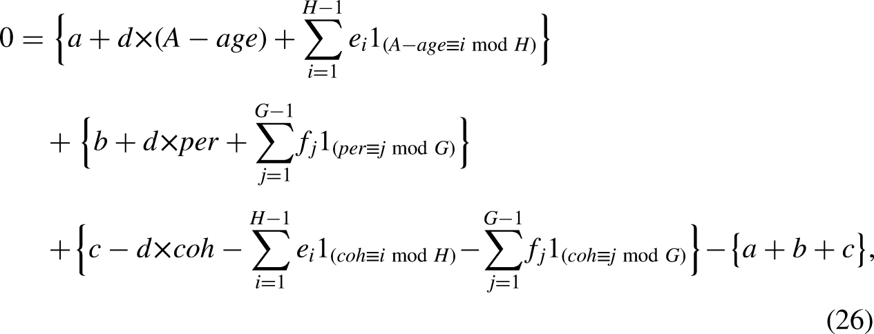

$$\begin{array}{rl}0& =\{a+d\times (A-age)+\sum _{i=1}^{H-1}{e}_i{1}_{(A-age\equiv i\mathrm{mod}H)}\}\\ & +\{b+d\times per+\sum _{j=1}^{G-1}{f}_j{1}_{(per\equiv j\mathrm{mod}G)}\}\\ & +\{c-d\times coh-\sum _{i=1}^{H-1}{e}_i{1}_{(coh\equiv i\mathrm{mod}H)}-\sum _{j=1}^{G-1}{f}_j{1}_{(coh\equiv j\mathrm{mod}G)}\}-\{a+b+c\},\end{array}$$

(26)

for any values of $a,b,c,d,e_i,f_j$ for $1\le i<H$ , $1\le j<G$ . The special case where $G>1$ , $H=1$ is covered by Riebler and Held (2010). The general result is from N22.

The transformations in (26) have dimension $G+H+2$ , see also Holford (2006: p. 983). This can be broken down as 4 macro effects and $G+H-2$ micro effects. The macro effects are the usual unidentified $3$ levels and $1$ slope associated with the coefficients $a$ , $b$ , $c$ , $d$ . The micro effects are $G-1$ period-cohort micro levels and $H-1$ age-cohort micro levels associated with the coefficients $e_i$ and $f_j$ . The macro and micro terminology relate to the discussion of Holford (2006).

When it comes to the mixed-frequency two-sample case, we will want to characterize the transformations of the time effects that leave the predictor ${\mu }_{age,per,s}$ in (24) unchanged. Identity (26), applied for each sample $s=1,2$ , implies that the dimension of the variation of the predictor is

$$p=q-2(G+H+2)=2\{A_G+P_H+A+P-(G+1)(H+1)\}.$$

(27)

Invariant reparameter

The next step is to find invariant parameters. Holford (2006) discusses this in terms of macro effects and micro effects and argues that standard double differences will not be invariant, but explicit formulas are not given. Instead we build on N22. Following the approach for the regular case, we will describe the relevant double differences at first and then the relevant linear planes.

Non-linear invariant components. Following N22, we define double differences as follows. Let ${\mathrm{\Delta }}_H$ indicate $H$ -period differencing so that ${\mathrm{\Delta }}_H{\beta }_{per,s}={\beta }_{per,s}-{\beta }_{per-H,s}$ . Correspondingly, let ${\mathrm{\Delta }}_G$ indicate $G$ -period differencing that will be used for age effects. We also require $GH$ -differencing ${\mathrm{\Delta }}_{GH}$ to describe macro effects. We form second differences

$$\begin{array}{rl}{\mathrm{\Delta }}_{GH}{\mathrm{\Delta }}_H{\beta }_{per,s}& ={\mathrm{\Delta }}_{GH}{\beta }_{per,s}-{\mathrm{\Delta }}_{GH}{\beta }_{per-H,s}\\ & ={\beta }_{per,s}-{\beta }_{per-H,s}-{\beta }_{per-GH,s}+{\beta }_{per-GH-H,s}.\end{array}$$

(28)

These double differences can be expressed in terms of the predictor as

$${\mathrm{\Delta }}_{GH}{\mathrm{\Delta }}_H{\beta }_{per,s}={\mu }_{age,per,s}-{\mu }_{age,per-H,s}-{\mu }_{age-GH,per-GH,s}+{\mu }_{age-GH,per-GH-H,s}.$$

(29)

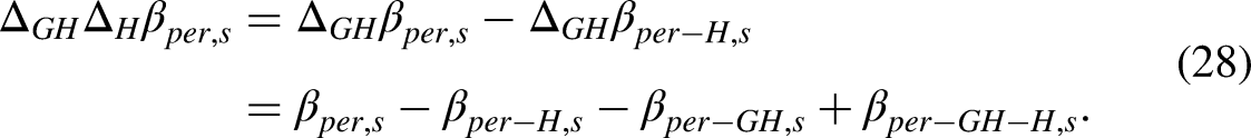
The double differences ${\mathrm{\Delta }}_{GH}{\mathrm{\Delta }}_H{\beta }_{per,s}$ are invariant. Why? The period index moves in steps of $H$ . Thus, $H$ -double differencing ${\mathrm{\Delta }}_H^2$ is needed to eliminate the linear trend $b+d\times per$ in (26). The term $\sum _{j=1}^{G-1}{f}_j{1}_{(per\equiv j\mathrm{mod}G)}$ in (26) comes about because of the grouping on the age scale. This could be eliminated by $G$ -differencing was it not for fact that period develops in $H$ -steps. Since $G$ and $H$ have no common divisors, a macro $GH$ -difference is needed to elimate the period grouping effects. Overall, we must combine $GH$ and $G$ differences to achive invariance.

The simpler one-period double differences ${\mathrm{\Delta }}_1{\mathrm{\Delta }}_1{\beta }_{per}$ are invariant in the regular case $G=H=1$ , but not invariant in general as pointed out by Holford (2006), Gascoigne and Smith (2023). Likewise, $H$ -double differences ${\mathrm{\Delta }}_H^2{\beta }_{per}$ are only invariant when $G=1$ .

For the age effect, we will by a similar argument use double differences ${\mathrm{\Delta }}_{GH}{\mathrm{\Delta }}_G{\alpha }_{age,s}$ . For the cohort effect the situation is slightly easier because cohorts move in steps of 1. Therefore, it suffices to use ${\mathrm{\Delta }}_G{\mathrm{\Delta }}_H{\gamma }_{coh,s}$ differences. The possible indices for the cohort double differences are

$${\mathcal{I}}_{coh}\circ =(G+2H,\dots ,C)\mathrm{\setminus }(G+2H+c,C-c:c\in {\mathcal{N}}_{G,H}).$$

(30)

The number of possible cohorts in this set is $C-(2H+G-1)-2S_{G,H}$ , which equals $A+P-GH-G-H$ . The full set of invariant double differences is

$${\mathrm{\Delta }}_{GH}{\mathrm{\Delta }}_G{\alpha }_{age,s}\text{f}orage=A-gG\text{w}ith0\le g\le A_G-H-2,$$

(31)

$${\mathrm{\Delta }}_{GH}{\mathrm{\Delta }}_H{\beta }_{per,s}\text{f}orper=H+hH\text{w}ithG+1\le h\le P_H-1,$$

(32)

$${\mathrm{\Delta }}_G{\mathrm{\Delta }}_H{\gamma }_{coh,s}\text{f}orcoh\in {\mathcal{I}}_{coh}\circ .$$

(33)

The dimension of this set of double differences is $2(G+H+1)$ less than $p$ , given in (27), as we have $A_G-H-1$ ages, $P_H-G-1$ periods and $A+P-GH-G-H$ cohorts.

Linear invariant components. N22 finds linear invariant components as follows. We have levels

$${\mu }_{A,H,s}={\alpha }_{A,s}+{\beta }_{H,s}+{\gamma }_{H,s}+{\delta }_s,$$

(34)

and invariant age-cohort and period-cohort parameters

$$\begin{array}{rl}{\lambda }_{g,s}& ={\mu }_{A-gG,H}-{\mu }_{A,H}\\ & ={\mathrm{\Delta }}_{gG}{\gamma }_{H+gG,s}-{\mathrm{\Delta }}_{gG}{\alpha }_{A,s}\text{f}org=1,\dots ,H,\end{array}$$

(35)

$$\begin{array}{rl}{\nu }_{h,s}& ={\mu }_{A,H+hH}-{\mu }_{A,H}\\ & ={\mathrm{\Delta }}_{hH}{\gamma }_{H+hH,s}+{\mathrm{\Delta }}_{hH}{\beta }_{H+hH,s}\text{f}orh=1,\dots ,G.\end{array}(36)$$

(36)

We will later interpret ${\lambda }_{H,s}$ as a age-cohort slope and ${\nu }_{G,s}$ as a period-cohort slope. The parameters ${\lambda }_{g,s}$ for $s<H$ and ${\nu }_{h,s}$ for $s<G$ will give micro effects in the level of predictor. The dimension of these components is $2(G+H+1)$ as required.

Full set of invariant components. We combine the double differences, levels and slopes in a vector $\xi =({\xi }_1^{\prime },{\xi }_2^{\prime }{)}^{\prime }$ , where

$$\begin{array}{rl}{\xi }_s& =({\mu }_{A,H,s};{\lambda }_{g,s}\text{f}or1\le g\le H;{\nu }_{h,s}\text{f}or1\le h\le G;\\ & {\mathrm{\Delta }}_{GH}{\mathrm{\Delta }}_G{\alpha }_{A-gG}\text{f}or{A}_G-H-2\ge g\ge 0;\\ & {\mathrm{\Delta }}_{GH}{\mathrm{\Delta }}_H{\beta }_{H+hH}\text{f}orG+1\le h\le P_H-1;\\ & {\mathrm{\Delta }}_G{\mathrm{\Delta }}_H{\gamma }_{coh}\text{f}orcoh\in {\mathcal{I}}_{coh}\circ {)}^{\prime }.\end{array}$$

(37)

The parameter $\xi$ has the desired dimension $p$ as given in (27).

Writing the predictor in terms of invariant parameters

The next step is to write the predictor in terms of the invariant parameters. This serves two purposes: To given an interpretation of the model and to derive a design matrix. The added difficulty is to deal with the mixed frequency. Here we rely on N22. We start by defining macro and micro steps in the time scales.

Macro and micro steps in the time scales. A key observation in N22 is to express the time scales through their Euclidean representations. This gives a way of formulating Holford’s macro and micro steps in an explicit and general way.

Age moves in micro steps of length $G$ , but we are also interested in macro steps of length $GH$ . The Euclidean reprentation of $A-age=gG$ is as follows. The largest number of macro steps is $q_g=\lfloor g/H\rfloor$ , which is the largest integer not exceeding $g/H$ . There is remainder of $r_g=g-q_{g}H$ micro steps. Hence, $age=A-q_{g}GH-r_{g}G$ . Similarly, for period, let $q_h=\lfloor h/G\rfloor$ and $r_h=h-q_{h}G$ . Thus, we can write the three time scales as

$$\begin{array}{rl}age& =A-q_{g}GH-r_{g}G,per=H+q_{h}GH+r_{h}H,\\ coh& =H+(q_g+q_h)GH+r_{g}G+r_{h}H.\end{array}$$

(38)

The Euclidean representations is vizualized by Table 1 where $G=5$ and $H=3$ . The macro steps are $GH=15$ . Italic and roman font indicate the macro blocks. We see that cohort 18 appears in the top right corner of two macro blocks. This is where the remainders for age and period are both zero, $r_g=r_h=0$ . Macro effects link these values. Within each macro block there are $GH$ different combinations of remainder terms. Each of these give a micro effect. Such macro and micro effects are perceived in Holford (2006) but are entirely explicit. Thus, we rely on N22 henceforth.

Representation of predictor. We are now ready to represent the predictor in terms of the invariant parameters. The representation depends on the macro steps $q_g$ , $q_h$ and the micro steps $r_g$ , $r_h$ in the above Euclidean representation (38) through

$$\begin{array}{rl}{\mu }_{age,per,s}=& \{{\mu }_{A,H,s}+1_{(r_g>0)}{\lambda }_{r_g,s}+1_{(r_h>0)}{\nu }_{r_h,s}\}+q_g{\lambda }_{H,s}+q_h{\nu }_{G,s}\\ & +S_{q_g,r_g,s}^{age}+S_{q_h,r_h,s}^{per}+S_{q_g,q_h,r_g,r_h,s}^{coh}.\end{array}$$

(39)

The expressions for the non-linear terms $S_{q_g,r_g,s}^{age}$ , $S_{q_h,r_h,s}^{per}$ and $S_{q_g,q_h,r_g,r_h,s}^{coh}$ are given in (A.13), (A.15) and (A.16) in Appendix A.3 in the online Supplemental Material. As before, the practical value of the details of this formula lies in the production of computer code. The interpretation can largely be gleaned from the above expression.

The mixed-frequency representation (39) has a more complicated appearance than that for the regular case in (16). This is because of the micro steps associated with the different values of $r_g$ , $r_h$ , where we recall that $0\le r_g<H$ and $0\le r_h<G$ . The overall picture is that we get a regular representation for each value of $r_g$ , $r_h$ . Indeed, the representations have nearly identical notation for $r_g=r_h=0$ and exactly identical notation if we also let $G=H=1$ . We will refer to the $r_g=r_h=0$ representation as the macro representation, whereas each $r_g$ , $r_h$ combination is a micro representation.

A closer inspection of the mixed-frequency representation (39) reveals that certain components are common across different values of $r_g$ , $r_h$ . The linear slopes in (39) are remarkably simple as the age-cohort slopes ${\lambda }_{H,s}$ and the period-cohort slopes ${\nu }_{G,s}$ do not vary with micro effects. The slopes are multiplied with $q_g$ and $q_h$ , which measure time in macro steps.

Turning to the level term in curly brackets in (39), we see different levels for different $r_g$ and $r_h$ combinations. In the macro representation with $r_g=r_h=0$ , the level is given by ${\mu }_{A,H,s}$ . For other $r_g$ , $r_h$ combinations, the level is adjusted by age-cohort parameters ${\lambda }_{r_g,s}$ for $0<r_g<H$ and period-cohort parameters ${\nu }_{r_h,s}$ for $0<r_h<G$ . Note that this list of parameters does not include the slopes ${\lambda }_{H,s}$ and ${\nu }_{G,s}$ discussed above. Moreover, when $G$ , $H$ are both larger than unity, then the $GH$ different slopes are not freely varying as they are formed from only $G+H-1<GH$ parameters.

The non-linear age term $S_{q_g,r_g,s}^{age}$ in (39) depends on age time through $q_g$ , $r_g$ , but is constant across period time. The exact expression in (A.15) in Appendix A.3 in the online Supplemental Material indicates that the age term may not develop smoothly between macro steps. Some further comments on this issue will be given below.

The non-linear period term $S_{q_h,r_h,s}^{per}$ in (39) has a structure that is similar to that of the age term. It varies with period time but it is constant in age time.

The non-linear cohort term $S_{q_g,q_h,r_g,r_h,s}^{coh}$ in (39) varies both with age time and with period time. The exact expression in (A.16) has a rather complicated micro variation across different $r_g$ , $r_h$ .

Some comments on apparent seasonality in non-linear terms. The representation helps us in thinking about the identified parts of the time effects. A particular issue is that estimates of the non-linear time effects may give an impression of seasonality as observed by Holford (2006) and Riebler and Held (2010).

The age, period and cohort double differences in (A.13), (A.15), (A.16) measure curvature in the predictor. In general, we would expect the predictor to be smooth, so that double differences are non-zero but small. Thus, we would only expect slightly different period-cohort slopes for different values of $r_h$ .

In practice, parameters are estimated. Data will typically not be entirely smooth due to random noise or model error. Because of the large number of parameters, the fit will track the data quite well, but with quite volatile double differences. If the underlying double difference parameter is small corresponding to a smooth predictor, its signal will be dominated by the double difference estimation error. In particular, if the double difference parameters are zero, as in a linear plane model, their estimates can be quite volatile. When cumulated, such estimation errors can generate an impression of seasonality as observed. The seasonal patterns may be constant over time or varying over time. There is a considerable literature on seasonality in time series econometrics, with a distinction between deterministic and stochastic seasonality (Ghysels and Osborn 2001; Hylleberg et al. 1990). Such distinctions are of interest if the seasonality is part of the signal. But the seasonality is perhaps of less interest when it is driven mainly by estimation error. This seems to be the case in the present situation. We will return to these points in the data example.

Design matrix. With the representation, we can construct design vectors $x_{age,per}$ for each sample as for the regular case. Again, these design vectors are common accross samples and can be combined across samples as we saw in (18). The main purpose remains computational: To code the model in a statistical package, and to compute and plot the predictor and its constituents. This is done in the apc package for R (Nielsen 2015).

Invariance and identification conditions. Finally, we must check the conditions $(a)$ – $(c)$ from §3.2.4. $(a)$ holds since $\xi$ is an invariant function of $\mu$ . For instance, the period double differences are expressed in terms of $\mu$ in (29) and their invariance is argued just after (29). Similar results apply for the age and cohort double differences. The level and slopes are expressed in terms of $\mu$ in (34)–(36). $(b)$ holds since $\mu$ is expressed in terms of $\xi$ in (39) through the terms (A.13)-(A.16). $(c)$ is checked in Theorem 1 of N22.

Hypotheses on Common Time Effects

Hypotheses on common time effects can be formulated for the mixed case in a similar fashion as for the regular case.

In the unrestricted model the predictors are expressed in terms of the canonical parameters through the representation in (39). From this we can extract a design vector $x_{age,per}$ that is common for the two samples. We get a representation of the predictor in terms of design vectors and canonical parameters ${\xi }_s$ for each sample just as in (18). Hypotheses that restrict time effects to be common can then be imposed on the cross-sample differences $({\xi }_2-{\xi }_1)/2$ as before. The main hypotheses are as follows.

Hypothesis	Restriction	Degrees of freedom
Common age effect	${\mathrm{\Delta }}_{GH}{\mathrm{\Delta }}_G{\alpha }_{age,1}={\mathrm{\Delta }}_{GH}{\mathrm{\Delta }}_G{\alpha }_{age,2}$	$A_G-H-1$
Common period effect	${\mathrm{\Delta }}_{GH}{\mathrm{\Delta }}_H{\beta }_{per,1}={\mathrm{\Delta }}_{GH}{\mathrm{\Delta }}_H{\beta }_{per,2}$	$P_H-G-1$
Common cohort effect	${\mathrm{\Delta }}_G{\mathrm{\Delta }}_H{\gamma }_{coh,1}={\mathrm{\Delta }}_G{\mathrm{\Delta }}_H{\gamma }_{coh,2}$	$A+P-GH-G-H$
Common external period effect		$P_H-G-2$
	${\mathrm{\Delta }}_{GH}{\mathrm{\Delta }}_G{\beta }_{per,2}-{\mathrm{\Delta }}_{GH}{\mathrm{\Delta }}_G{\beta }_{per,1}=\psi {\mathrm{\Delta }}_{GH}{\mathrm{\Delta }}_G{T}_{per}$

Further submodels can be formulated as for the regular case, see also N22.

Empirical Illustration

We now consider the Swiss suicide data reviewed earlier. A two-sample age-period-cohort predictor will be applied in the context of a log-normal model using least squares for the log rates. We will first analyze the two samples separately using one-sample age-period-cohort analyses. All time effects will appear significant. The scale parameters are found to be different across samples. Correction for this difference will be done through generalized least squares regression combined with a small-dispersion asymptotic theory. We will then find that we cannot reject the hypothesis of a common period effect. We will also explore the use of a marriage-divorce index as period effect.

The data analysis was done in R (R Core Team 2022) using code building on the apc package (Nielsen 2015).

Initial One-sample Analyses

At first, we model the two samples separately using 1-sample mixed-frequency age-period-cohort analyses. We assume that the log rate is normal, where the expectation has a linear age-period-cohort structure as in (24) and constant variance. The models are estimated using least squares. For inference we can, at this point, rely on the exact distribution theory for the normal model.

Tables 2 and 3 show separate standard 1-sample analyses of variance for women and for men. Each table consider 1-sample APC models and reductions to 1-sample sub-models AP, AC and PC where, respectively, the cohort, the period and the age effects are omitted. Thus, in Table 2, APC refers to a standard 1-sample age-period-cohort model for women while AP refers to a standard 1-sample age-period submodel for women. All restrictions are strongly rejected. We note that the residual standard deviation, $\hat{\sigma }$ , is smaller for women than for men, matching the lower number of cases for women.

Table 2.

Analysis of variance, women.

Model	Test vs APC
	$-2\log L$	df	F	df	$p_F$	$\hat{\sigma }$
APC	$-363.02$	572				0.218
AP	$-157.38$	684	1.60	112	0.0002	0.229
AC	$68.82$	624	5.25	52	0.0000	0.254
PC	$-18.55$	583	30.11	11	0.0000	0.272
${\chi }_{normality}^2(2)=4.50$ $(p=0.105)$ .

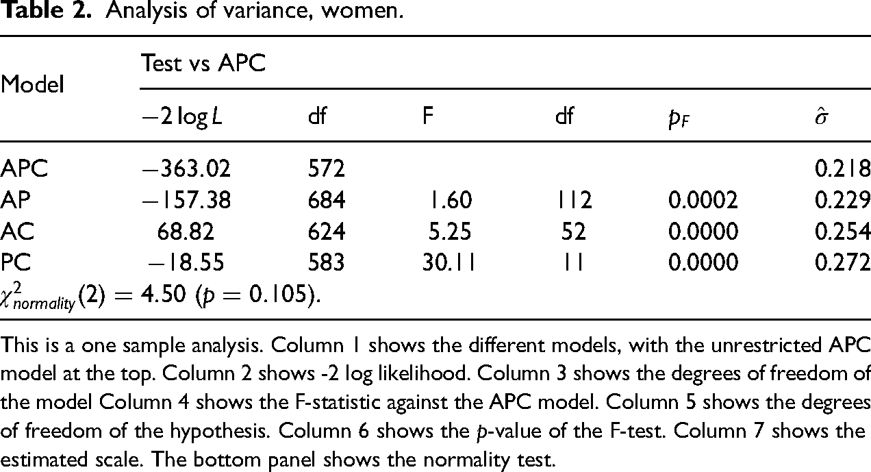
This is a one sample analysis. Column 1 shows the different models, with the unrestricted APC model at the top. Column 2 shows -2 log likelihood. Column 3 shows the degrees of freedom of the model Column 4 shows the F-statistic against the APC model. Column 5 shows the degrees of freedom of the hypothesis. Column 6 shows the $p$ -value of the F-test. Column 7 shows the estimated scale. The bottom panel shows the normality test.

Table 3.

Analysis of variance, men. The table is structured as Table 2.

Model	Test vs APC
	$-2\log L$	df	F	df	$p_F$	$\hat{\sigma }$
APC	$-841.70$	572				0.159
AP	$-605.48$	684	1.88	112	0.0000	0.170
AC	$-434.27$	624	7.88	52	0.0000	0.199
PC	$-210.52$	583	68.10	11	0.0000	0.239
${\chi }_{normality}^2(2)=0.35$ $(p=0.839)$ .

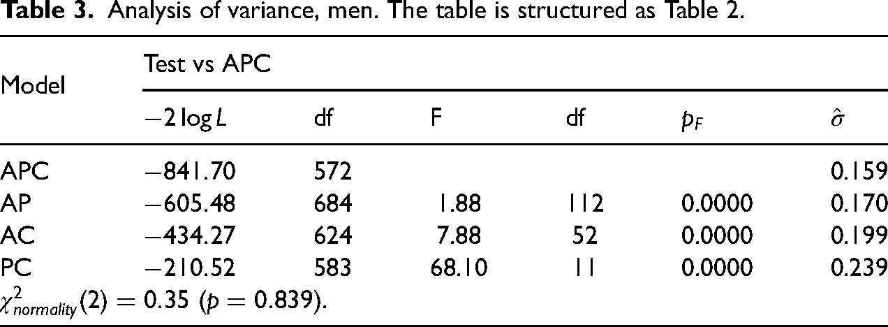
Tables 2 and 3 also show tests for the normality assumption. The tests are standard skewness and kurtosis based tests, see for instance Hendry and Nielsen (2007). In both cases, the $p$ -values are large and the assumption of normality cannot be rejected.

Two-sample Analysis by Least Squares

We apply the proposed two-sample age-period-cohort analysis, where the common predictor is unrestricted while the cross-sample differenced predictor is restricted in various ways. The log normal specification is maintained. We consider both the case with common scale parameter so that least squares estimation can be used and the case of different scale parameters in the two samples so that generalized least squares estimation is needed. Table 4 summarizes the results. Thus, APC refers to the unrestricted two-sample age-period-cohort model. Further, AP refers to the sub-model where the common predictor is an unrestricted APC model where the cross-sample difference is an AP model, so that the non-linear cohort effect is restricted to be common for women and men, while all other effects are unrestricted.

Table 4.

Two-sample analysis of variance.

Model	Test vs APC
diff.	$-2\log L_{GLS}$	df	F	df	$p_F$	${\hat{\sigma }}_{OLS}$	${\hat{\sigma }}_{GLS}$
APC	$-1129.99$	1144				0.191	0.159
AP	$-836.72$	1256	2.19	112	0.0000	0.201	0.167
AC	$-1052.62$	1196	1.16	52	0.2092	0.192	0.160
PC	$-1021.68$	1155	7.74	11	0.0000	0.197	0.164
OLS: ${\chi }_{normality}^2(2)=15.82$ $[p=0.0004]$
GLS: ${\chi }_{normality}^2(2)=2.13$ $[p=0.3440]$

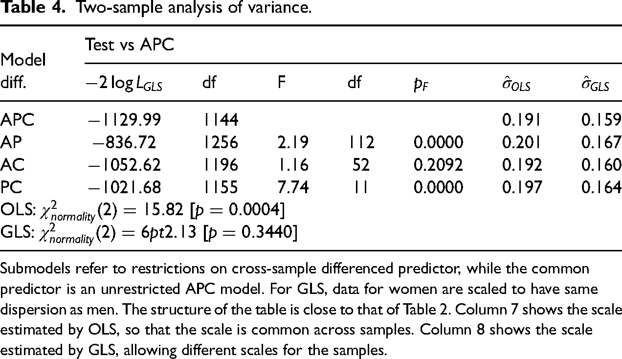
Submodels refer to restrictions on cross-sample differenced predictor, while the common predictor is an unrestricted APC model. For GLS, data for women are scaled to have same dispersion as men. The structure of the table is close to that of Table 2. Column 7 shows the scale estimated by OLS, so that the scale is common across samples. Column 8 shows the scale estimated by GLS, allowing different scales for the samples.

Inference relies on asymptotic arguments. We must specify the assumptions underlying the asymptotics. One approach is to let the size of the data array and therefore the size of the parameter vector increase as in Fu (2016). Another approach is to use small-dispersion asymptotics, where the size of the data array is kept fixed while the scale, or dispersion, parameters are shrinking in the asymptotic experiment. The second approach seems particular useful here as the dose, or exposure, is large. The dose is the entire Swiss population of the relevant age and gender. It is in the order of 100,000 for each cell. With the second approach it is possible to justify use of F distributions as limiting distributions. Formal analysis is given by Jørgensen (1987) in the context of exponential dispersion models whereas Harnau and Nielsen (2018) develop a Central Limit Theorem for this situation. Both setups allow log normal distribution, but the latter has some flexibility in allowing approximate log normal distributions and some types of over-dispersed Poisson models. The implementation in Kuang and Nielsen (2020) is suited for the present situation. Thus, the idea of the asymptotic experiment is that log suicide rates converge to constant parameters for large values of the dose appearing as denominator of the rates. Convergence of the rates to constant parameters corresponds to a shrinking dispersion. More specifically, we apply a log normal model where we hold fixed the dimension of the index array, the canonical age-period-cohort parameter, and the ratio of the scales in the samples, while the scale parameters shrink in the asymptotic experiment.

The common variance assumption can be tested by comparing the least squares log likelihoods for the APC model in Table 4 and in Tables 2 and 3 to get the Bartlett test statistic (Harnau 2018; Kuang and Nielsen 2020). The test statistic is $363.02+841.70-1129.99=78.73$ multiplied by a Bartlett correction factor which is very close to unity in this case. The test statistic is large compared to a ${\chi }_1^2$ -distribution. In addition, normality is rejected. This is quite possibly a consequence of mixing two samples with different scale. Ordinary least squares will therefore not give reliable inference. Instead, generalized least squares is needed. This is done by scaling the log rates and the design matrix for women by the ratio of the scale estimates for men and women as reported in Tables 2 and 3. This results in a scaling factor of $0.159/0.218$ . We see that normality can no longer be rejected.

We now consider the restrictions on the age-period-cohort structure for the differenced predictor. The F-statistics for the three sub-models considered in Table 4, turn out to be exactly identical when estimating by ordinary least squares and by generalized least squares. This is a consequence of the particular block structure of the design and covariance matrices and can be checked through a somewhat detailed derivation. However, given the difference in dispersion for women and men, we must apply the F-statistics under the generalized least squares setup. In that case the F-statistics are asymptotically F-distributed under the small-dispersion setup. Thus, from Table 4 we learn that we can reduced the model for the cross-sample differenced predictor to an age-cohort model, whereas the age-period and period-cohort models are strongly rejected. The interpretation of the age-cohort model is that the period effect is common across samples. This matches conclusions by Riebler et al. (2012).

Plots of Macro Time Effects

Plots of the time effects will give us more insight in the age-period-cohort variation in suicide rates. In the present mixed frequency situation, we start with the macro effects, where interpretations are strongest. The macro effects are affected by arbitrary linear trends in the same ways as for regular data. Thus, the graphs will be detrended to minimize the confusion over the arbitrary linear trends.

Figure 2 shows macro time effects deduced from the initial one-sample age-period-cohort models, discussed in §5.1. The reason for showing the one-sample plots as opposed to the plots in models with cross-sample restrictions imposed is as follow. In the empirical analysis one will start by looking at the one-sample plots to gain insight into the data and the model. This then motivates the choice of testable cross-sample restrictions. By using the invariant parametrization, estimates of the remaining parameters should not change very much as long as the restrictions are statistically valid. Above, it has been discussed whether to replace the cross-sample period effect with an external time series or to remove it entirely. Each will give a slight variation in the plots. This variation seems less interesting than the formal tests that were carried out above.

On the left, effects are shown for each sample. On the right, the cross-sample differences are shown. Solid lines are estimates, dotted lines are $\pm 2$ standard errors around zero. Standard errors are centred at zero in order to support inferences that are concerned with zero restrictions. By construction, the standard errors are exactly proportional for the two samples. The proportionality factor reflects the different dispersion across samples.

The plots are constructed as follows. We start by computing the non-linear effects $S_{q_g,0,s}^{age}$ , $S_{q_h,0,s}^{per}$ and $S_{q_g,q_h,0,0,s}^{coh}$ from the representation (39) and where the remainders are set to zero $r_g=r_h=0$ . These move along in macro steps. All three series are detrended to start and end in zero.

The actual computation of the effects $S_{q_g,0,s}^{age}$ , $S_{q_h,0,s}^{per}$ and $S_{q_g,q_h,0,0,s}^{coh}$ is relatively simple. In the regression analysis, the design matrix has a row for each observation and a column for each invariant parameter. For the age effect, we select those rows corresponding to macro steps of $age$ and the smallest value of period, that is $r_g=0$ and $h=0$ , and those columns corresponding to the relevant age double differences as defined in (A.15).

Detrending serves three purposes. First, to emphasize non-linearity, which is the only part of the time effects that is invariant to the identification problem. Second, to disentangle the plots, so that they can be viewed separately. Indeed, with fewer constraints the plots are linked inextricably and must be viewed jointly (Carstensen 2007). Third, to ensure that the degrees of freedom shown in the plot matches the degrees of freedom associated with the time effects. Detrending can be done in various ways. Here, time effects are restricted to be zero at the beginning and at the end. There is no estimation uncertainty at those two points and the degrees of fredom can be appreciated. One can then focus on the shapes in the pictures, such as skew concave shapes for age and S-shape for period. Chauvel and Schröder (2014) suggest to set the averaged time effect to zero and then eliminate the time trend. This achieves the first two objectives above.

Figure 2, first row, shows the two detrended age effects. We will look for global and local peaks and the general shape of the age effects. Peaks indicate ages at which there is a relative acceleration in the prevalence of suicide. With the two-sample analysis we can get an insight into how these peaks differ for women and men. The non-linear age effects should come more clearly out in Figure 2 than in the raw data plots in Figure 1, where age effects are contaminated by period-cohort effects. With aggregate data one will of course only be able to conclude that one should seek to understand why these peaks arise using other sources of information.

The one-sample detrended age effects first rise considerably. This corresponds to a relatively large increase in suicide rates for people in their twenties. The curves then decline gradually corresponding to relative declines in rates. There are small local peaks around the age of 50 and for men also at age 75. The age-effects are significant for both men and women in line with the individual tests for the period-cohort models in Tables 2 and 3. The plot on the right shows the (women-men) difference of the age trends. This is also significantly different from zero in line with the rejection of the PC model in Table 4.

Figure 2, second row, shows detrended macro period effects, detrended to start and end in zero. Once again, we see that the period effects are individually significant, although somewhat less than for ages, in line with the tests for the age-cohort models reported in Tables 2 and 3. The difference plot indicates that the period-trends follow each other in line with the non-rejectance of the AC model in Table 4.

Figure 2, third row, shows detrended cohort macro effects. Again, restricted to start and end in zero. Overall, the individual cohort effects are less significant than age and period effects – compare with the age-period tests in Tables 2 and 3. The cohort effects are somewhat different across samples in line with Table 4.

The plots of the detrended age and cohort macro effects resemble the plots in Figure 5 of Riebler et al. (2012). Two features of the original plots are worth pointing out. First, macro detrending and micro demeaning was not applied in the age plots, so the reader will have to do an occular adjustment to interpret the plots correctly. Second, the cohorts were smoothed over macro and micro effects, which are subject to the transformations in (26).

Plots of Micro Time Effects

We now consider plots of the micro effects. The micro effects are affected by arbitrary levels, but not not by linear trends.

Figure 3 shows demeaned micro effects. Micro effects only occur for the period and cohort effects as $G=1$ but $H=5>1$ in the present situation. The subfigures of Figure 3 are organized similar to Figure 2, so that the rows concern period and cohort, respectively. The first column shows the two one-sample estimates, with their difference shown in the second column.

We construct the micro effects along the principles for constructing the macro effects. For period micro effects for $j=1,\dots ,G-1$ are found by computing the differences $S_{q_h,r_j,s}^{per}-S_{q_h,0,s}^{per}$ . Demeaning is done by starting each micro difference in zero. In the plots, the micro effects belonging to the same macro block are connected with lines. The cohort micro effects are constructed along the same lines.

We observe seasonal patterns as discussed in §4.2.1 and by previous authors including Holford (2006), Riebler and Held (2010). We note that the seasonal pattern is nearly constant over time for the cohort effects, but changing somewhat over time for the period effects and in particular for women. It is possible that seasonal patters mainly generated by estimation error or model error, see §4.2.1. Indeed, the vertical variation within each macro block is modest relative to the shown confidence bands.

Replacing the Period Effect with an External Time Series

We now investigate if the period effect can be replaced by an external time series. Following Riebler et al. (2012), we consider a family integration index computed as $(m_{per}-d_{per})/(m_{per}+d_{per})$ where $m_{per}$ and $d_{per}$ are the counts of marriages and divorces in a given period. The F-index is shown in Figure 4. A high value of this measure indicates better integration which could be associated with lower suicide rate.

The hypothesis that the period effect follows the F-index only concerns the non-linear parts, see Section ‘Replacing period effect with time series’. Thus, we implement the restriction by substituting the double differences of the period effect with those of the F-index. Table 5 gives an analysis of variance. Here, the common predictor and the cross-sample differenced predictor are restricted either individually or jointly. The first model has an age-period-cohort structure for both predictors. The third model has an age-cohort structure for the cross-sample differenced predictor. The second model sits in between the two models and allows a period effect following the F-index for the cross-sample differenced predictor.

Table 5.

Two-sample analysis of variance.

Model			Test vs APC			Test vs AC+F
diff.	$-2\log L_{GLS}$	df	F	df	$p_F$	F	df	$p_F$	${\hat{\sigma }}_{OLS}$	${\hat{\sigma }}_{GLS}$
APC	$-1129.99$	1144							0.191	0.159
AC+F	$-1058.80$	1195	51	1.084	0.321				0.191	0.159
AC	$-1052.62$	1196	52	1.158	0.209	1	4.906	0.027	0.192	0.160

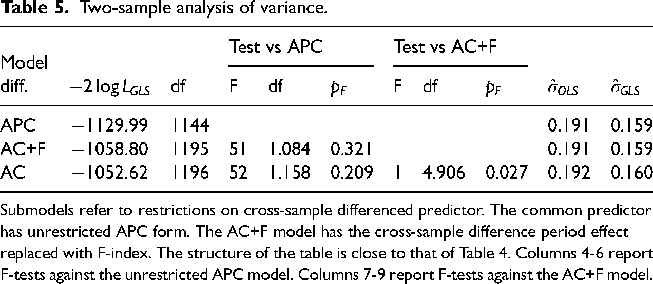
Submodels refer to restrictions on cross-sample differenced predictor. The common predictor has unrestricted APC form. The AC+F model has the cross-sample difference period effect replaced with F-index. The structure of the table is close to that of Table 4. Columns 4-6 report F-tests against the unrestricted APC model. Columns 7-9 report F-tests against the AC+F model.

The conclusion from the table is that we cannot reject replacing the period effect of the cross-sample differenced parameter with the F-index. Eliminating the F-index from that model to get an age-cohort structure adds another degree of freedom. The relevant F-statistic is 4.906 with p-value 2.7%, which gives a marginal decision. Thus, there is slight evidence that it is better to replace the period effect in the difference parameter with the F-index than eliminating it all together. The coefficient $\psi$ for the F-index is estimated by $-0.217$ with standard error $0.098$ . The first sample is chosen as women. Thus, changes in family integration has a $21.7\mathrm{\%}$ larger impact for men than for women. This is in line with conclusions by Riebler et al.

Conclusions

We considered the linear two-sample age-period-cohort model. The main contribution is the analysis of the two-sample age-period-cohort problem for regular and for mixed frequency data. The age-period-cohort predictors are linear combinations of different time effects as in (4). The age, period and cohort time scales are linked through the identity (2) which leads to the age-period-cohort problem that the linear parts of the age, period and cohort effects can be altered by moving arbitrary linear trends between age, period and cohort effects. For regular data, this is described by the transformation identity (6). There are two aspects to the age-period-cohort problem: identification and invariance.

The identification problem is essentially a collinearity problem, where parameters cannot be estimated uniquely. A common approach is to remove the collinearity by imposing sufficiently many restrictions on the design matrix. However, this will in general not solve the invariance problem.

The invariance problem relates to interpretation. Two investigators may solve the identification problem by imposing different restrictions on the design matrix. They will then find different linear parts of the estimated age, period and cohort effects. The solution is to focus on parameters that are invariant to the pernicuous linear trend manipulations. This argument goes back to Fienberg and Mason (1979). The contribution of this paper is to extend this to a characterization of all invariant parameters and reparametrize the model exclusively in terms of the invariant parameter (15). This removes the age-period-cohort problem as in the one-sample analyses by Kuang et al. (2008) and Martínez Miranda et al. (2015).

The consequence of the analysis is that all interpretation and inference should be based on the non-linear parts of the age, period and cohort effects or the combination of their linear parts. In contrast, one cannot learn about the individual linear effects from the data. As an example, in the context of two samples for women and for men, the non-linear period effects are interpretable for each sample, whereas the linear period effects are not. One can compare the period effects across samples and one may impose a restriction of common period effects across samples. Even so, all individual linear effects remain sensitive to transformations by arbitrary linear terms. In the extreme case where the predictor is restricted to zero across age, period and sample, the linear age, period and cohort effects remain illusive due to the transformation identity (6).

Graphical representation of the age, period and cohort effects brings the age-period-cohort problem back. It is important to remember that such graphs can be altered arbitrarily due to the transformations in (6). Thus one should focus on deviation from linearity rather than linear trends. This can be done by detrending the age, period and cohort effects separately. Here, we detrended by ensuring that each of the (macro) graphs start and end in zero, so that one can focus on shapes instead of slopes.

The two-sample model could be appealing in many sociological studies. In the suicide example, the initial analysis was to apply standard one-sample age-period-cohort analysis to each of the two sample for women and for men. By graphical inspection one got the impression that the period effects are similar. This was tested formally using a two-sample analysis. These ideas will be relevant in many sociological contexts, where investigators have hitherto conducted separate one-sample analyses without being able to test cross sample restrictions. The outcomes could be crime rates, attitudes, social mobility, obesity, fertility or mortality. The stratification could be done by sex, racial group, parental social class or country.

Some studies use more than two samples. Jacobsen et al. (2004) compared female mortality in Danmark, Norway and Sweden. Held and Riebler (2012) analyzed chronic obstructive pulmonary disease mortality for England and Wales stratified by sex and by three regions. Rosenberg and Miranda-Filho (2024) considered cancer surveillance for many US samples. The transformation identity (6) and the invariant parameter (15) generalize to situations where the sample index $s$ takes several values. The challenge would be to write code that keeps track of multiple samples. In practice, one should of course be careful not to stratify so much that the information in each age, period cell becomes too diluted.

A feature of the presented analysis is that it focuses on the parametrization. The results can therefore be transferred to a wide range of statistical models. In the suicide example, the chosen model was a log-normal model combined with the small-dispersion inference (Harnau and Nielsen 2018). For other types of data the invariant parametrization could be embedded in a Poisson regression, where over-dispersion may be handled by the small-dispersion idea, or perhaps a Binomial regression. If the data consists of repeated cross-sections, one could make a two-sample version of the model in Fannon et al. (2021). Some comments on Bayesian implementation are given in Appendix A.4 in the online Supplemental Material.

The presented analysis of the two-sample age-period-cohort problem was extended to mixed frequency data. The transformation identity (26) is then more complicated and results in macro and micro effects as described by Holford (2006) and the invariant parameter has the more complicated expression (15). A hypothesis of common non-linear effects across samples is tested by a linear restriction on the parameters. Graphs of the macro effects are interpretable in a similar fashion as for regular data. In the suicide example, the interpretation of the micro effects was less clear. Future analysis of other data may bring some light on the interpretation of micro effects.

To conclude all interpretation and inference should rest exclusively on the non-linear age, period and cohort effects and on the combined linear plane(s). With the invariant parametrization, the practitioner can focus on just this with the benefit of only have to use standard regression techniques.

Supplemental Material

sj-pdf-1-smr-10.1177_00491241251376509 - Supplemental material for Two-sample Age-period-cohort Models

Supplemental material, sj-pdf-1-smr-10.1177_00491241251376509 for Two-sample Age-period-cohort Models by Bent Nielsen in Sociological Methods & Research

Supplemental Material

sj-pdf-2-smr-10.1177_00491241251376509 - Supplemental material for Two-sample Age-period-cohort Models

Supplemental material, sj-pdf-2-smr-10.1177_00491241251376509 for Two-sample Age-period-cohort Models by Bent Nielsen in Sociological Methods & Research