Beyond the Diagonal Reference Model: Critiques and New Directions in the Analysis of Mobility Effects

Abstract

Over the past decade there has been a striking increase in the number of quantitative studies examining the effects of social mobility, with almost all based on the diagonal reference model (DRM). We make four main contributions to this rapidly expanding literature. First, we show that under plausible values of mobility effects, the DRM will, in many cases, implicitly force the underlying mobility linear effect toward zero. In addition, we show both mathematically and through simulations that the mobility effects estimated by the DRM are sensitive to the size and sign of the origin and destination linear effects, often in ways that are unlikely to be intuitive to applied researchers. This finding clarifies why, contrary to expectations, applied researchers have generally found mixed evidence of mobility effects. Second, we generalize the identification problem of conventional mobility effect models by showing that the DRM and related methods can be viewed as special cases of a bounding analysis, where identification is achieved by invoking extremely strong assumptions. Finally, and importantly, we present a new framework for the analysis of mobility tables based on the identification and estimation of joint parameter sets, introducing what we call the structural and dynamic inequality model. We show that this model is fully identified, relies on much weaker assumptions than conventional models of mobility effects, and can be treated both as a descriptive model and, if additional assumptions are invoked, as a causal model. We conclude with an agenda for further research on the consequences of socioeconomic mobility.

Introduction

Interest in the consequences of social mobility (SM) is longstanding (for reviews see Hendrickx et al. 1993; Hope 1971, 1975). From its earliest days, the scientific literature on SM, or the experience of moving up or down the class hierarchy of a given society, has debated its individual-level effects. For example, the sociologist Pitirim Sorokin (1927) hypothesized negative effects of not just downward but also upward SM on individual wellbeing, as those who reach a status different from that of their parents may suffer from the cultural gap between their attained position and their family origins (see also Friedman 2016). Nearly a century later, there is a large body of quantitative sociological research that has sought to estimate the direct effects of the experience of SM on a wide range of individual outcomes, including well-being (e.g., life satisfaction, stress, allostatic load, and substance abuse), attitudes (e.g., trust, political ideology, and redistribution preferences), and behaviors (e.g., voting, fertility, and health behaviors) (see also Appendix A, supplemental materials). The inconsistent (and often small) mobility effects that this literature has estimated appear to refute longstanding sociological theory and present a general challenge to much of the work on SM undertaken by sociologists. Since the influential work of Lipset and Bendix (1959), researchers have carried out a number of important and widely cited studies exploring differences in rates of SM across and within countries (e.g., Bloome 2015; Chetty et al. 2014; Erikson and Goldthorpe 1992; Grusky and Hauser 1984). To the extent that a high degree of social fluidity is considered a normatively desirable aim (for a critical perspective see Swift 2004), these studies provide important descriptive evidence on the degree of openness of a given society or place. However, as Lipset and Zetterberg (1959) pointed out, “unless variations in mobility rates and in the subjective experience of mobility make a difference for society or for the behavior pattern of an individual, knowledge concerning rates of mobility will be of purely academic interest” (p. 6). Based on today’s quantitative evidence, it would seem that generations of sociologists and demographers have been trying to explain an outcome that is, on the whole, of little consequence to the individual.

Progress in empirically identifying the effects of SM on individuals has been hampered by a fundamental methodological challenge. Observed SM (M) is simply the difference between an individual’s social destination (D), such as their own social class, and their social origin (O), such as their parents’ social class, so that $M=D-O$ . As a result, any model of mobility effects that seeks to estimate the independent effects of social origins, social destinations, and the difference between them, that is, SM, is underidentified and cannot be estimated using conventional statistical techniques (Manski 1990, 2003). In contrast to problems of statistical inference, which involve understanding how sampling variability can affect conclusions based on samples of limited size, problems of identification entail understanding what conclusions can be drawn even with a sample of unlimited size. The lack of a unique solution of mobility effects is a classic identification problem, because it cannot be resolved by collecting larger samples.

To estimate such effects, a variety of techniques have been proposed, but the most popular approaches are those developed by the sociologists Otis Dudley Duncan (1966) and Michael Sobel (1981, 1985). A first wave of research, influenced by Duncan's (1966) square additive model (SAM), a basic two-factor origin-destination model with residual interaction terms, found no effect of SM on a number of outcomes (see also Hope 1971, 1975). This is partly explained by the fact that Duncan’s proposed model assumes that the linear effect of mobility is zero, as was recognized by at least some social scientists at the time (Blalock 1967:794-795). Another wave of research resulted from Sobel’s (1981, 1985) diagonal reference model (DRM), ¹ which is seen as the “gold standard” for mobility effects research (Houle and Martin 2011:197; Präg and Richards 2018:5; Sieben 2017). The statistician Sir David Cox (1990), for example, has lauded the DRM as an exemplar of “directly substantive” models in statistical analysis (p. 170). In recent years, sociologists have used Sobel’s model to explain a wide range of outcomes, including subjective well-being, political extremism, obesity, and so on (the list is too long to include here but see Appendix A, supplemental materials). However, as we show, like Duncan’s model, the DRM relies on very strong assumptions about the effects of SM.

This article is organized as follows. First, we outline the identification challenge, clarifying what can be known about the data from a mobility table with as few assumptions as possible. We make explicit how, under a general model of mobility effects, the nonlinear effects are identified and the linear effects are not. Second, we discuss the mathematical properties of the DRM, revealing that the DRM generates different mobility linear effects depending on both the size and sign of the linear and nonlinear effects of origin and destination. In doing so, we revisit Sobel’s (1981) findings on fertility and show that his data are consistent with a wide range of very large negative as well as positive linear mobility effects, none of which are recovered by the DRM. Third, we generalize models of mobility effects, showing how any existing mobility model that attempts to identify unique “effects” can be viewed as a special case of a bounding approach, except with extremely narrow bounds and thus extremely strong assumptions. Finally, we outline a new framework for analyzing mobility data using what we call the structural and dynamic inequality (SDI) model. Using this model, we demonstrate how one can describe both dynamic (or mobility-based) inequalities as well as those that are purely structural (reflecting an absence of SM). As we discuss, these estimates can also be interpreted as joint causal effects, and, therefore, involve much weaker assumptions than estimates from conventional models of mobility effects. We conclude with a programmatic statement outlining guidelines for further research on the individual-level consequences of SM.

I The DRM

As noted in the introduction, by far the most common approach to model mobility effects is the DRM developed by the sociologist Michael Sobel (1981, 1985). This popularity is indicated by the spike in recent works using the DRM to estimate mobility effects, as shown in Figure 1. It is also demonstrated by the widespread agreement in the literature on the importance and utility of the DRM for understanding the consequences of SM. For instance, Houle and Martin (2011:197) note, the DRM is “the only method used in modern mobility effects research.” Likewise, Sieben (2017) writes that DRMs “are thought to be the best solution to [the identification] problem.” Präg and Richards (2018:5) echo this claim, correctly stating: “A consensus is emerging in the literature that the diagonal reference model is superior to other modeling approaches and results based on other approaches are questionable at best.”

Figure 1.

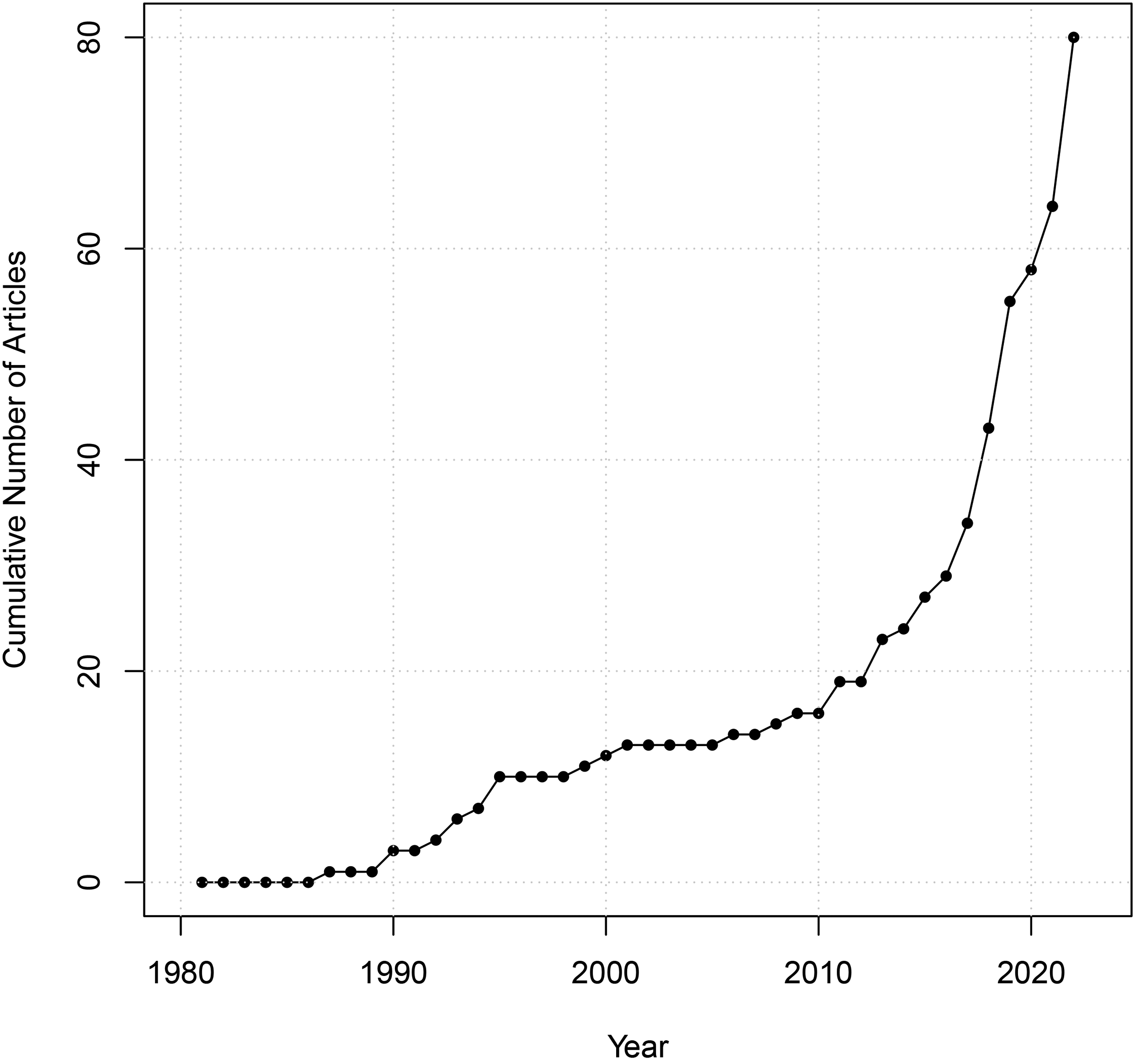
The rise of the diagonal reference model (DRM). Note: This line plot shows, by year, the cumulative number of articles using the DRM since Sobel’s (1981) publication. Appendix A, supplemental materials, contains the full list of publications that make up the data for this graph.

There is similarly widespread agreement that the DRM is effective in separating out the effects of mobility from those of origin and destination. For example, Schuck and Steiber (2018:1249) write that the DRM “tests for the net effects of intergenerational mobility over and above the effects of educational origin and destination, finally allowing mobility effects to be separated from mere level effects [emphasis in original].” Unfortunately, however, the DRM relies on extremely strong assumptions and, absent additional information external to the data, there is no reason to think that the model will actually recover the “true” underlying effect of mobility.

In this section, we first outline the basic mathematical properties of the DRM. As we illustrate, the DRM assumes that the origin and destination effects are proportional to each other, and thus we will refer to this assumption as the “proportionality constraint” (see also Weakliem 1992:157). Failure to satisfy this constraint may lead to erroneous estimates of the overall effects of origin, destination, and mobility. This is true of the linear effects, but also of the nonlinear effects, which, as noted above, are identified. ² Second, we revisit Sobel’s (1981) fertility data and show, mathematically and with simulations, that the DRM will fix the mobility linear effect at a very specific value even when the underlying mobility linear effect is extremely positive or negative. This is another way of stating that the proportionality constraint may hold for the nonlinear effects, but still not hold for the linear effects. Unfortunately, the data are not themselves informative about whether or not this constraint is satisfied. Finally, we develop a simple formula that, when the proportionality constraint is satisfied, clarifies the nature of the bias of the estimated mobility linear effect. As we show, the mobility linear effect generated by DRM is a function of the size, sign, and shape of the origin and destination effects. It is only under very specific conditions, namely when the ratio of the origin and destination weights equals the ratio of the underlying origin and destination linear effects, that the DRM will recover the true underlying mobility linear effect.

1. Overview of the DRM

To orient the discussion that follows, suppose we have a set of categorical variables for $i=1,\dots ,I$ origin groups, $j=1,\dots ,J$ destination groups, and k  =  1, $\dots$ , K mobility groups, where $k=j-i+I\text{and}K=I+J-1$ . The fundamental model of mobility effects can be specified using what we call the classical origin–destination–mobility (C-ODM) model:

$$Y=f(O^{*},D^{*},M^{*})+ϵ=\mu +{\alpha }_i+{\beta }_j+{\gamma }_k+{\eta }_{ijk}+{\xi }_{rijk},$$

(1)

where $\mu$ is the intercept (or overall mean); ${\alpha }_i$ , ${\beta }_j$ , and ${\gamma }_k$ denote the $i\mathrm{th}$ , $j\mathrm{th}$ , and $k\mathrm{th}$ observed levels of origin, destination, and mobility, respectively; ${\eta }_{ijk}$ is an additional (orthogonal) term denoting interactions; and ${\xi }_{rijk}$ is an individual-level, normally distributed error term with a mean of zero. As we discuss in Appendix B in the supplemental material, equation (1) is based on the implicit assumption that O, D, and M (and their respective indices) can be treated as surrogates for distinct causal variables $O^{*}$ , $D^{*}$ , and $M^{*}$ (and their respective indices). To simplify the exposition, we will accordingly refer to ${\alpha }_i$ , ${\beta }_j$ , and ${\gamma }_k$ as the “true” origin, destination, and mobility effects, but the reader should keep in mind that this is shorthand, as detailed in Appendix B, supplemental materials, for referring to the causal effects ${\alpha }_l^{*}$ , ${\beta }_p^{*}$ , and ${\gamma }_n^{*}$ (for a similar point, see Fosse and Winship 2019a).

An alternative formulation of the C-ODM model (see equation (1)) helps clarify the nature of the identification problem. By orthogonalizing the linear from the nonlinear terms, we can specify what we call the linearized origin–destination–mobility (L-ODM) model:

$$\begin{array}{r}{\mu }_{rijk}=\mu +\alpha (i-i*)+\beta (j-j*)+\gamma (k-k*)+{\tilde{\alpha }}_i+{\tilde{\beta }}_j+{\tilde{\gamma }}_k+{\eta }_{ijk}+{\xi }_{rijk}\end{array},$$

(2)

where the asterisks denote midpoint or referent indices $i*=(I+1)/2$ , $j*=(J+1)/2$ , and $k*=(K+1)/2$ ; $\alpha$ , $\beta$ , and $\gamma$ denote the linear effects of origin, destination, and mobility, respectively; and $\tilde{\alpha }$ , $\tilde{\beta }$ , and $\tilde{\gamma }$ represent the origin, destination, and mobility nonlinear effects, respectively; ${\eta }_{ijk}$ is, as before, an additional (orthogonal) term denoting interactions; and ${\xi }_{rijk}$ is a normally distributed individual-level error term with a mean of zero. To identify the levels of the parameters given the inclusion of the intercept, sum-to-zero constraints are applied to the linear and nonlinear parameters. The L-ODM greatly simplifies the nature of the identification problem, allowing us to show how the DRM makes highly specific assumptions about the unknown origin, destination, and mobility linear effects. Moreover, as we show later, it allows one to use graphical tools for visualizing and partially identifying the parameters of a mobility effects model.

The L-ODM highlights that the core identification challenge resides in the linear effects ( $\alpha ,\beta ,\mathrm{and}\gamma$ ). The DRM, the most prevalent method used to address this challenge and estimate distinct mobility effects, achieves point identification by imposing highly specific identifying constraints with respect to these linear effects. To understand this, it is crucial to recognize that the DRM is a nonlinear model in that at least one of the (unknown) model parameters are a nonlinear function of at least one of the other (unknown) model parameters. By contrast, conventional linear regression is linear in the parameters, although it can be parameterized so that it is nonlinear in the variables. The general form for a nonlinear regression model is as follows:

$$y_r=f({\mathbf{x}}_r,\theta \theta )+{ϵ}_r,$$

(3)

where $r=1,\dots ,R$ indexes the rows (e.g., individuals) of the data set, $q=1,\dots ,Q$ the number of variables in the model, and $p=1,\dots ,P$ the number of parameters; $y_r$ is the outcome of the rth row; f is a known function; ${\mathbf{x}}_r$ is a $Q\times 1$ column vector of variables $x_{1r},\dots ,x_{Qr}$ ; $\theta \theta$ is a $P\times 1$ column vector of parameters ${\theta }_1,\dots ,{\theta }_P$ ; and ${ϵ}_r$ is an error term. ³

Suppose we have a data set based on aggregated data from a mobility table with rows indexed by $r=1,\dots ,R=I\times J$ . The DRM is a particular kind of nonlinear model that begins with the following as a baseline model:

$${\mu }_{ijk}=f({\mathbf{x}}_r,\theta \theta )=w_o{\mu }_{i[j=i]}+w_d{\mu }_{[i=j]j}+{\varphi }_{ijk},$$

(4)

with

$$w_o=\frac{e^{{\xi }_1}}{e^{{\xi }_1}+e^{{\xi }_2}}\mathrm{and}{w}_d=1-w_o=\frac{e^{{\xi }_2}}{e^{{\xi }_1}+e^{{\xi }_2}},$$

where ${\mu }_{ijk}$ is the mean outcome for a particular cell on the mobility table indexed by i and j (with $k=j-i+I$ ); $w_o$ is the class origin weight; $w_d$ is the class destination weight, which is equal to $1-w_o$ ; ${\xi }_1$ and ${\xi }_2$ are the origin and destination parameters, respectively, used to calculate the weights; ${\mu }_{i[j=i]}$ and ${\mu }_{[i=j]j}$ are the diagonal means of the mobility table indexed by class origin and destination, respectively; and ${\varphi }_{ijk}$ is a cell-specific error term. ⁴

Above the baseline model, mobility effects can be parameterized as a set of categorical variables:

$${\mu }_{ijk}=w_o{\mu }_{i[j=i]}+w_d{\mu }_{[i=j]j}+{\gamma }_k+{\varphi }_{ijk},$$

(5)

where ${\gamma }_k$ denotes the set of mobility effect parameters using, say, sum-to-zero deviation coding. Sobel (1981:902) suggests that mobility effects are present whenever the ${\gamma }_k$ ’s in equation (5) are statistically significant. ⁵

The DRM as outlined in equation (5) and applied to a three-by-three mobility table is shown in Table 1. The joint origin and destination effects for the cells on the main diagonal, representing non-mobile groups, are given by the estimates of ${\mu }_{i[j=i]}$ (or, equivalently, ${\mu }_{[i=j]j}$ ). ⁶ For example, if there are I = 3 origin categories and J = 3 destination categories, as is the case in Table 1, then the joint origin and destination effects on the main diagonal are given by ${\mu }_{11}$ , ${\mu }_{22}$ , and ${\mu }_{33}$ . The joint origin and destination effects for the cells off the main diagonal, representing mobile groups, are given by $w_o{\mu }_{i[j=i]}+w_d{\mu }_{[i=j]j}$ , where $w_o$ and $w_d$ can be interpreted as the relative salience of the origin and destination categories, respectively. For instance, as shown in Table 1, the joint effects for origin and destination in the cell i = 2 and j = 1 are given by $w_o{\mu }_{22}+w_d{\mu }_{11}$ .

Table 1.

Diagonal Reference Model on a $3\times 3$ Mobility Table.

	j = 1	j = 2	J = 3
i = 1	${\mu }_{113}={\mu }_{11}+{\gamma }_3+{\varphi }_{113}$	${\mu }_{124}=w_{\text{o}}{\mu }_{11}+w_{\text{d}}{\mu }_{22}+{\gamma }_4+{\varphi }_{124}$	${\mu }_{135}=w_{\text{o}}{\mu }_{11}+w_{\text{d}}{\mu }_{33}+{\gamma }_5+{\varphi }_{135}$	K = 5
i = 2	${\mu }_{212}=w_{\text{o}}{\mu }_{22}+w_{\text{d}}{\mu }_{11}+{\gamma }_2+{\varphi }_{212}$	${\mu }_{223}={\mu }_{22}+{\gamma }_3+{\varphi }_{223}$	${\mu }_{234}=w_{\text{o}}{\mu }_{22}+w_{\text{d}}{\mu }_{33}+{\gamma }_4+{\varphi }_{234}$	k = 4
I = 3	${\mu }_{311}=w_{\text{o}}{\mu }_{33}+w_{\text{d}}{\mu }_{11}+{\gamma }_1+{\varphi }_{311}$	${\mu }_{322}=w_{\text{o}}{\mu }_{33}+w_{\text{d}}{\mu }_{22}+{\gamma }_2+{\varphi }_{322}$	${\mu }_{333}={\mu }_{33}+{\gamma }_3+{\varphi }_{333}$	k = 3
	k = 1	k = 2	k = 3

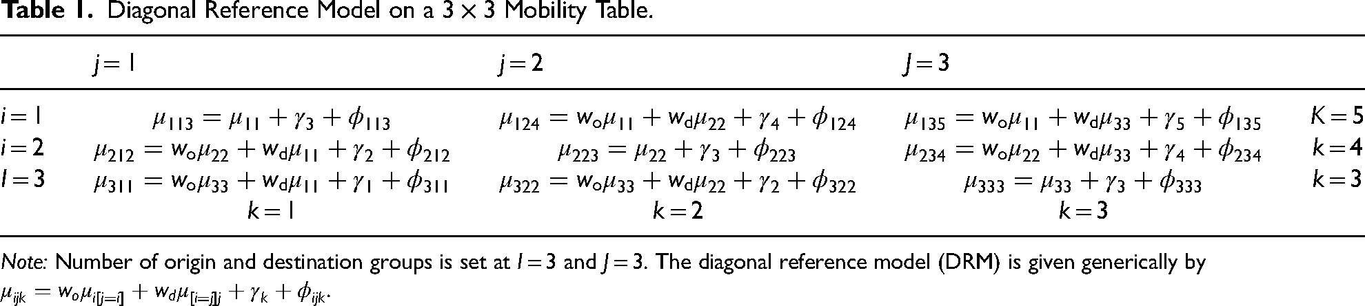
Note: Number of origin and destination groups is set at I = 3 and J = 3. The diagonal reference model (DRM) is given generically by ${\mu }_{ijk}=w_o{\mu }_{i[j=i]}+w_d{\mu }_{[i=j]j}+{\gamma }_k+{\varphi }_{ijk}$ .

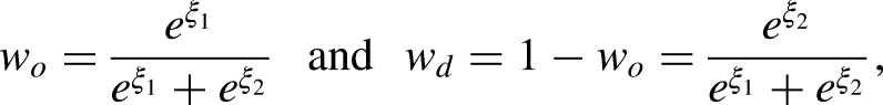
To understand the underlying mathematical properties of the DRM, it is useful to describe the weights needed to recover the underlying origin, destination, and mobility effects. ⁷ The true means on the main diagonal after adjusting for the mobility effects can be written as (cf. equation (2)):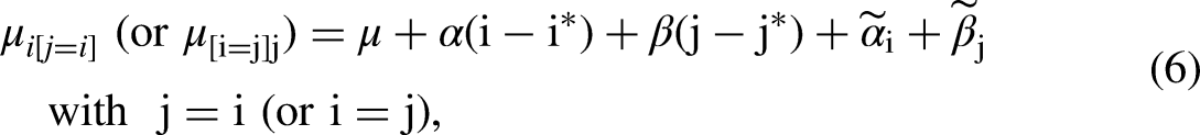

$${\mu }_{i[j=i]}(\text{or}{\mu }_{[i=j]j})=\mu +\alpha (i-i^{*})+\beta (j-j^{*})+{\tilde{\alpha }}_i+{\tilde{\beta }}_j\text{with}j=i(\text{or}i=j),$$

(6)

where $\mu$ is the overall mean; $\alpha$ and $\beta$ are the true origin and destination mobility linear effects, respectively; ${\tilde{\alpha }}_i$ is the $i\text{th}$ origin nonlinear effect; ${\tilde{\beta }}_i$ is the $j\text{th}$ destination nonlinear effect; $i^{*}=(I+1)/2$ and $j^{*}=(J+1)/2$ . Note again that we assume that, to identify the intercept, we have applied sum-to-zero constraints on the origin, destination, and mobility effects.

The weight required to recover the true contribution of the ith origin effect is as follows: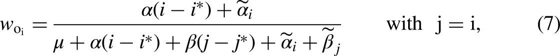

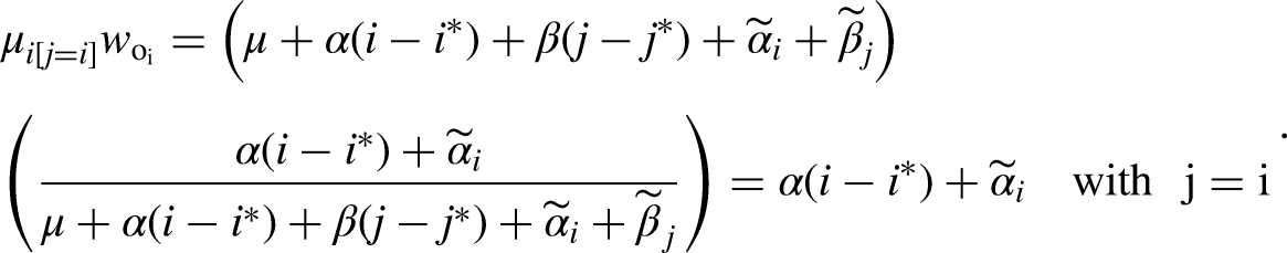
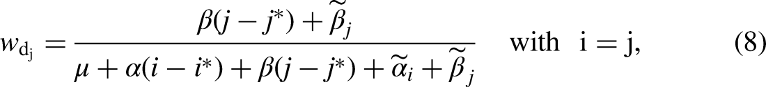
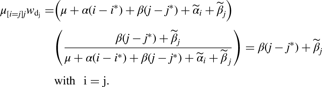
$$w_{{\text{o}}_i}=\frac{\alpha (i-i^{*})+{\tilde{\alpha }}_i}{\mu +\alpha (i-i^{*})+\beta (j-j^{*})+{\tilde{\alpha }}_i+{\tilde{\beta }}_j}\text{with}j=i,$$

(7)

where $w_{{\text{o}}_i}$ is the weight of the ith origin category. Then multiplying this weight by the main diagonal means (equation (6)) will generate the ith origin effect:

$$\begin{array}{rl}& {\mu }_{i[j=i]}{w}_{{\text{o}}_i}=(\mu +\alpha (i-i^{*})+\beta (j-j^{*})+{\tilde{\alpha }}_i+{\tilde{\beta }}_j)\\ & (\frac{\alpha (i-i^{*})+{\tilde{\alpha }}_i}{\mu +\alpha (i-i^{*})+\beta (j-j^{*})+{\tilde{\alpha }}_i+{\tilde{\beta }}_j})=\alpha (i-i^{*})+{\tilde{\alpha }}_i\text{with}j=i\end{array}.$$

Similarly, the actual weight required to recover the true value of the $j\text{th}$ destination effect is

$$w_{{\text{d}}_j}=\frac{\beta (j-j^{*})+{\tilde{\beta }}_j}{\mu +\alpha (i-i^{*})+\beta (j-j^{*})+{\tilde{\alpha }}_i+{\tilde{\beta }}_j}\text{with}i=j,$$

(8)

where $w_{{\text{d}}_j}$ is the weight of the jth destination category. Multiplying this weight by the main diagonal means (equation (6)) will generate the jth destination effect as follows:

$$\begin{array}{rl}{\mu }_{[i=j]j}{w}_{{\text{d}}_j}=& (\mu +\alpha (i-i^{*})+\beta (j-j^{*})+{\tilde{\alpha }}_i+{\tilde{\beta }}_j)\\ & (\frac{\beta (j-j^{*})+{\tilde{\beta }}_j}{\mu +\alpha (i-i^{*})+\beta (j-j^{*})+{\tilde{\alpha }}_i+{\tilde{\beta }}_j})=\beta (j-j^{*})+{\tilde{\beta }}_j\\ & \text{with}i=j.\end{array}$$

Crucially, the weights in equations (7) and (8) are unknown, because they require knowledge of the unidentified origin and destination linear effects. Note further that the weights are allowed to vary across class and destination origins, respectively, and there is no restriction that the weights sum to one (or some other value).

By contrast, the DRM’s proportionality constraint means that we assume that the origin and destination effects can be characterized by a single origin weight (or, equivalently, destination weight). In essence, the DRM attempts to recover the true origin and destination effects (and, accordingly, the true mobility effects) by splitting the main diagonal cells of a mobility table into origin and destination components. More specifically, the proportionality constraint assumes that the relative contributions of the linear and nonlinear origin effects with 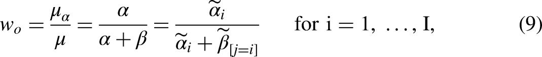$i=j$ are the same, and that the same relative proportion of the grand (or overall) mean is attributable to class origin. That is, with respect to the class origin weight, the DRM assumes the following: ⁸

$$w_o=\frac{{\mu }_{\alpha }}{\mu }=\frac{\alpha }{\alpha +\beta }=\frac{{\tilde{\alpha }}_i}{{\tilde{\alpha }}_i+{\tilde{\beta }}_{[j=i]}}\text{,for}i=1,\dots ,I,$$

(9)

where ${\mu }_{\alpha }$ is that part of the overall mean that is attributable to class origin. Similarly, the DRM assumes the following with respect to the class destination weights:

$$w_d=\frac{{\mu }_{\beta }}{\mu }=\frac{\beta }{\alpha +\beta }=\frac{{\tilde{\beta }}_j}{{\tilde{\alpha }}_{i=j}+{\tilde{\beta }}_j}\text{,for}j=1,\dots ,J,$$

(10)

where ${\mu }_{\beta }$ is that part of the overall mean that is attributable to class destination. This formulation implies that the origin and destination linear effects are of the same sign (or one of them is zero) such that the size of each linear effect is constrained to lie between 0 and $\alpha +\beta$ , inclusive.

Assuming the proportionality constraint defined in equations (9)–(10) holds, multiplying the main digaonal cells in equation (6) by the origin weight w _o yields the following set of origin effects:

$${\mu }_{i[j=i]}{w}_{\text{o}}=\mu w_o+[(\alpha +\beta )w_o](i-i^{*})+{\tilde{\alpha }}_i,$$

(11)

where $w_o$ is defined as in equation (9). Because $w_o={\mu }_{\alpha }/\mu$ as well as $\alpha /(\alpha +\beta )$ by (9), plugging either expression for w _o into equation (9) recovers ${\mu }_{\alpha }$ and $\alpha$ . Likewise, multiplying the main diagonal cells in equation (6) by the destination weight w _d yields the following set of destination effects:

$${\mu }_{[i=j]j}{w}_d=\mu w_d+[(\alpha +\beta )w_d](j-j^{*})+{\tilde{\beta }}_j,$$

(12)

where $w_d$ is defined as in equation (10). Similarly, because $w_d={\mu }_{\beta }/\mu$ as well as $\beta /(\alpha +\beta )$ by (10), substituting either expression for the destination weight w _d into equation (12) recovers ${\mu }_{\beta }$ and $\beta$ .

Under the proportionality constraint outlined in equations (9)–(10), simple formulas for calculating the origin, destination, and mobility linear effects can be derived. Specifically, the origin linear effect generated by the DRM is $\hat{\alpha }=(\alpha +\beta )w_o$ , and the estimated destination linear effect is $\hat{\beta }=(\alpha +\beta )w_d$ . ⁹ As well, the estimated mobility linear effect is given by $\hat{\gamma }=(\gamma -\alpha )+(\alpha +\beta )w_o$ or, equivalently, $\hat{\gamma }=(\gamma +\beta )-(\alpha +\beta )w_d$ . ¹⁰ However, again it should be emphasized that these calculations assume that the proportionality constraint holds or, equivalently, that the DRM weights equal the (unknown) true weights. Because the origin, destination, and mobility linear effects are not identified, the proportionality assumption with respect to the linear effects cannot be tested against the data: the plausibility of this assumption can only be justified by appealing to theory or substantive knowledge about the underlying processes of SM.

With actual data, the origin and destination weights estimated by the DRM (i.e., ${\hat{w}}_o$ and ${\hat{w}}_d$ , respectively) are a function of the underlying origin and destination nonlinear effects. Intuitively this makes sense, as these are identifiable components of the model while the linear effects are not. If the actual origin and destination nonlinear effects conform to the proportionality constraint, then the DRM’s estimated weights will correctly recover these underlying nonlinear effects. ¹¹ If there are no underlying origin, destination, and mobility nonlinear effects, then the DRM will generally produce origin and destination weights of ${\hat{w}}_o=0.500$ and ${\hat{w}}_d=0.500$ . In other words, absent additional information about the origin and destination linear effects, the DRM will, in general, assign equal value to the origin and destination categories with respect to the main diagonal cells of the mobility table. This is not an unreasonable assumption if there is no additional information available about the magnitude or direction of the linear effects, but researchers should be aware that it is an assumption nonetheless, and not an intrinsic feature of the data. We revisit this issue later when we discuss a generalization of bounding analyses for mobility effects models.

The above suggests a procedure for at least partially testing the plausibility of the proportionality constraint against the data. By fitting the L-ODM under a constraint, such as a zero destination linear effect, we can obtain a set of estimates of the underlying overall nonlinear effects of origin, destination, and mobility. We can then compare these nonlinear effects with those estimated by the DRM. If these are discrepant, then this suggests that the DRM is inappropriate, inasmuch it fails to recover the actual nonlinear effects. Alternatively, we can test whether or not the relative ratios of the origin and destination nonlinear effects are the same, as required by the DRM’s proportionality constraint (see equations (9) and (10)). For example, we can examine whether or not the ratio of the first origin nonlinear effect to the sum of the first origin and destination nonlinear effects is the same as the ratio of the second origin nonlinear effect to the sum of the second origin and destination nonlinear effects. If these ratios are the same, then this lends indirect support for the plausibility of the proportionality constraint. However, as we show below, even when the proportionality constraint holds with respect to the nonlinear effects, there is no guarantee that the DRM will recover the underlying mobility linear effect.

2. Sobel’s Fertility Findings Revisited

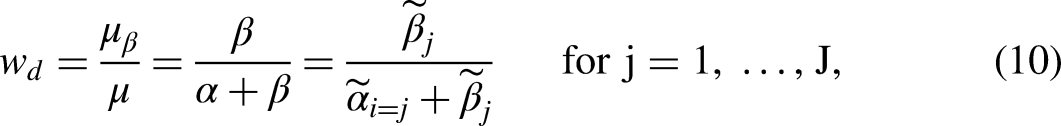
In this section, we re-examine Sobel’s (1981) findings on fertility using the DRM. We show that, even though the DRM assumes that there are virtually no mobility linear effects, the data are consistent with very large negative and positive linear effects. Sobel’s original data on fertility is shown in Table 2. The outcome is the average number of children ever born by father’s occupation (origin) and husband’s 1962 occupation (destination) among wives aged 42–61 years in March 1962 who were currently living with their husband in the Occupational Changes in a Generation (OCG) sample. The total sample size is $R=5,958$ .

Table 2.

Sobel (1981) Fertility Data.

	j = 1	j = 2	j = 3	j = 4	J = 5
i = 1	3.194	2.850	2.760	2.142	2.252	K = 9
	$(484)$	$(687)$	$(462)$	$(148)$	$(389)$
i = 2	3.000	2.423	2.423	1.908	2.180	k = 8
	$(34)$	$(513)$	$(345)$	$(163)$	$(322)$
i = 3	1.900	2.349	2.407	2.020	2.113	k = 7
	$(20)$	$(269)$	$(307)$	$(153)$	$(318)$
i = 4	2.700	2.225	2.389	1.631	2.005	k = 6
	$(10)$	$(71)$	$(54)$	$(65)$	$(190)$
I = 5	2.850	2.308	2.031	1.752	2.024	k = 5
	$(20)$	$(130)$	$(129)$	$(137)$	$(538)$
	k = 1	k = 2	k = 3	k = 4	k = 5

Note: The outcome is mean number of children ever born by father’s occupation (origin) and husband’s 1962 occupation (destination) among wives aged 42–61 years in March 1962 who were currently living with their husband in the OCG sample. Numbers in parentheses are the number of respondents for each cell. Total sample is $R=5,958$ .

We first examine the plausibility of the proportionality constraint assumed by the DRM in the case of Sobel’s fertility data. As noted in the previous section, this can be partially tested against the data because the nonlinear effects are identified. We first fit the L-ODM model by fixing the destination slope to zero, which allows us to estimate the nonlinear effects. These estimates, which are expressed as coefficients for orthogonal polynomials, ¹² are then converted to deviations from the grand (or overall) mean. We next fit the DRM and converted the estimated origin and destination effects into deviations orthogonal to their respective overall levels and linear components. 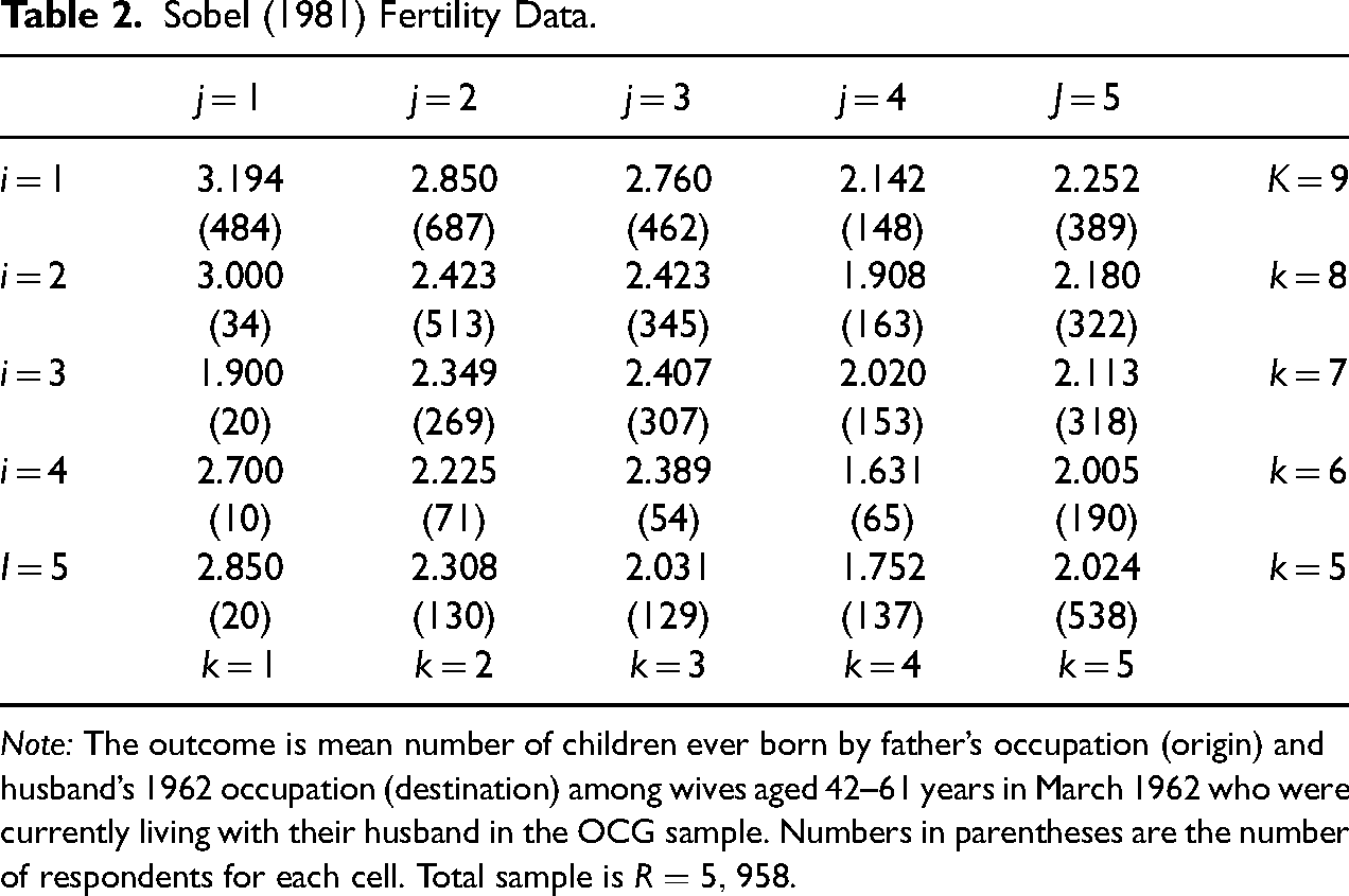¹³ Finally, for both models we calculated the estimated relative contributions of the origin and destination nonlinear effects. Specifically, for each model and for each of the origin nonlinear effects we calculated ${\tilde{\alpha }}_i/({\tilde{\alpha }}_i+{\tilde{\beta }}_{[j=i]})$ , while for each of the destination nonlinear effects we calculated ${\tilde{\beta }}_j/({\tilde{\alpha }}_{[i=j]}+{\tilde{\beta }}_j)$ . For example, the ith origin nonlinear effect is divided by the sum of the ith and jth origin and destination nonlinear effects.

Table 3 highlights the main findings with respect to our evaluation of the validity of the proportionality constraint. First, the nonlinear effects for origin and destination differ between the DRM and L-ODM model, in some cases substantially. On balance, however, in all cases but one the direction of the nonlinear effects is correctly captured by the DRM. Second, as shown in the second row of Table 3, with the DRM all of the ratios are the same for the origin and destination nonlinear effects. This reflects the fact that the estimated origin and destination weights for the DRM are $w_o=0.361$ and $w_d=0.639$ , respectively. Lastly, as shown in the bottom row of Table 3, the weights needed to recover the actual nonlinear effects, as represented by the estimates using the L-ODM model, vary considerably across origin and destination categories. This further suggests that the proportionality constraint of the DRM is likely inappropriate in this case.

Table 3.

Comparing Nonlinear Effects Using Data From Sobel (1981).

	Origin nonlinear effects					Destination nonlinear effects
	${\tilde{\alpha }}_1$	${\tilde{\alpha }}_2$	${\tilde{\alpha }}_3$	${\tilde{\alpha }}_4$	${\tilde{\alpha }}_5$	${\tilde{\beta }}_1$	${\tilde{\beta }}_2$	${\tilde{\beta }}_3$	${\tilde{\beta }}_4$	${\tilde{\beta }}_5$
DRM	0.085	$-0.078$	0.014	$-0.133$	0.112	0.150	$-0.139$	0.025	$-0.235$	0.199
Ratio	0.361	0.361	0.361	0.361	0.361	0.639	0.639	0.639	0.639	0.639
L-ODM model	0.122	$-0.119$	$-0.045$	$-0.038$	0.081	0.105	$-0.097$	0.069	$-0.265$	0.189
Ratio	0.538	0.552	$-1.918$	0.125	0.300	0.463	0.448	2.918	0.875	0.700

Note: Nonlinear effects for origin and destination are shown for the DRM and the L-ODM model using Sobel’s (1981) fertility data. Nonlinear effects for origin and destination, respectively, are expressed as deviations from their respective overall levels and linear effects. Ratios for the origin nonlinear effects are calculated as ${\tilde{\alpha }}_i/({\tilde{\alpha }}_i+{\tilde{\beta }}_{[j=i]})$ , while those for the destination nonlinear effects are calculated as ${\tilde{\beta }}_j/({\tilde{\alpha }}_{[i=j]}+{\tilde{\beta }}_j)$ . For example, the ith origin nonlinear effect is divided by the sum of the ith and jth origin and destination nonlinear effects. Total sample is $R=5,958$ . DRM = diagonal reference model; L-ODM = linearized origin–destination–mobility.

An additional issue is that even when the proportionality constraint of the nonlinear effects is valid, the DRM can generate highly biased estimates of the underlying mobility linear effect. This is the case even if the underlying mobility linear effect is extremely large. To show this, we conduct simulations based on the DRM and fertility data. Specifically, we fit the DRM and calculate the underlying estimated coefficients as linear and nonlinear effects, similar to the L-ODM. Then we use these to set up the data generating parameters (DGPs) in the simulations. Specifically, we first fix the origin, destination, and mobility linear effects to the values assumed by the DRM, which are $\alpha =-0.115$ , $\beta =-0.203$ , and $\gamma =-0.104$ . Then, we varied the values of mobility linear effect from $-1.000$ to $+1.000$ , while calculating values of the origin and destination linear effects that are consistent with the original fertility data. ¹⁴ The remaining DGPs are given by $\mu =2.3171$ , ${\alpha }^2=0.0411$ , ${\alpha }^3=0.0136$ , ${\alpha }^4=0.0161$ , ${\beta }^2=0.0730$ , ${\beta }^3=0.0242$ , ${\beta }^4=0.0285$ , ${\gamma }^2=-0.0012$ , ${\gamma }^3=-0.0074$ , ${\gamma }^4=0.0004$ , ${\gamma }^5=0.0027$ , ${\gamma }^6=-0.0022$ , ${\gamma }^7=0.0017$ , and ${\gamma }^8=-0.0008$ . In these simulations, like the Sobel data, we set the number of origin and destination groups at I = 5 and J = 5, respectively. We also replicated each combination of origin and destination (and accordingly mobility) groups so that number of individuals in each cell is identical to that of the original data. This resulted accordingly in a total sample size of $R=5,958$ for each simulation. For simplicity, and without loss of generality, we assume no random error.

The results from the simulations based on Sobel’s data are shown in Table 4. The table reveals that the DRM fixes the mobility linear effect to a particular value, $\hat{\gamma }=-0.010$ , even in cases in which the mobility linear effect is quite large (either negative or positive). The shaded column in Table 4 indicates that particular simulation in which the DRM recovers the true mobility linear effect. The results from this table underscores that the DRM can generate results that are, to a great degree, inconsistent with the true mobility effect. Note that in all simulated data sets the DRM correctly recovers the underlying nonlinear effects. This is by construction, as we have purposely created the data so that the DRM’s proportionality constraint on the nonlinear effects is valid.

Table 4.

Biased Mobility Linear Effects Using the DRM.

True DGP	$\gamma$	$-1.000$	$-0.500$	$-0.250$	$-0.010$	0.250	0.500	1.000
Origin effects	$\hat{\alpha }$	$-0.115$	$-0.115$	$-0.115$	$-0.115$	$-0.115$	$-0.115$	$-0.115$
	${\hat{\alpha }}^2$	0.041	0.041	0.041	0.041	0.041	0.041	0.041
	${\hat{\alpha }}^3$	0.0143	0.0143	0.0143	0.0143	0.0143	0.0143	0.0143
	${\hat{\alpha }}^4$	0.016	0.016	0.016	0.016	0.016	0.016	0.016
Destination effects	$\hat{\beta }$	$-0.202$	$-0.202$	$-0.202$	$-0.202$	$-0.202$	$-0.202$	$-0.202$
	${\hat{\beta }}^2$	0.073	0.073	0.073	0.073	0.073	0.073	0.073
	${\hat{\beta }}^3$	0.024	0.024	0.024	0.024	0.024	0.024	0.024
	${\hat{\beta }}^4$	0.029	0.029	0.029	0.029	0.029	0.029	0.029
Mobility effects	$\hat{\gamma }$	$-0.010$	$-0.010$	$-0.010$	$-0.010$	$-0.010$	$-0.010$	$-0.010$
	${\hat{\gamma }}^2$	$-0.001$	$-0.001$	$-0.001$	$-0.001$	$-0.001$	$-0.001$	$-0.001$
	${\hat{\gamma }}^3$	$-0.007$	$-0.007$	$-0.007$	$-0.007$	$-0.007$	$-0.007$	$-0.007$
	${\hat{\gamma }}^4$	$<0.001$	$<0.001$	$<0.001$	$<0.001$	$<0.001$	$<0.001$	$<0.001$
	${\hat{\gamma }}^5$	0.003	0.003	0.003	0.003	0.003	0.003	0.003
	${\hat{\gamma }}^6$	$-0.002$	$-0.002$	$-0.002$	$-0.002$	$-0.002$	$-0.002$	$-0.002$
	${\hat{\gamma }}^7$	0.002	0.002	0.002	0.002	0.002	0.002	0.002
	${\hat{\gamma }}^8$	$-0.001$	$-0.001$	$-0.001$	$-0.001$	$-0.001$	$-0.001$	$-0.001$

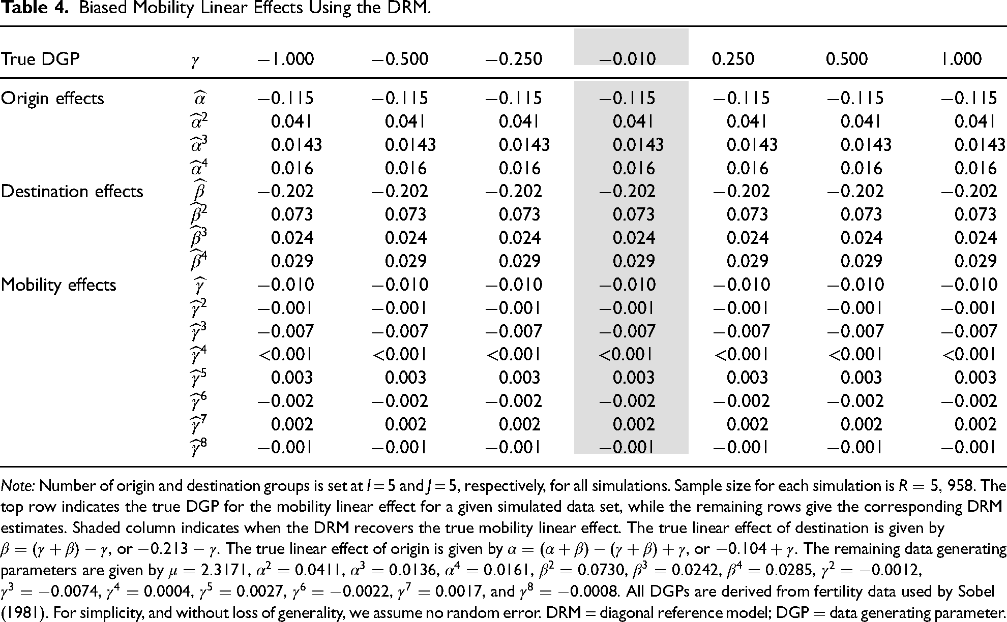
Note: Number of origin and destination groups is set at I = 5 and J = 5, respectively, for all simulations. Sample size for each simulation is $R=5,958$ . The top row indicates the true DGP for the mobility linear effect for a given simulated data set, while the remaining rows give the corresponding DRM estimates. Shaded column indicates when the DRM recovers the true mobility linear effect. The true linear effect of destination is given by $\beta =(\gamma +\beta )-\gamma$ , or $-0.213-\gamma$ . The true linear effect of origin is given by $\alpha =(\alpha +\beta )-(\gamma +\beta )+\gamma$ , or $-0.104+\gamma$ . The remaining data generating parameters are given by $\mu =2.3171$ , ${\alpha }^2=0.0411$ , ${\alpha }^3=0.0136$ , ${\alpha }^4=0.0161$ , ${\beta }^2=0.0730$ , ${\beta }^3=0.0242$ , ${\beta }^4=0.0285$ , ${\gamma }^2=-0.0012$ , ${\gamma }^3=-0.0074$ , ${\gamma }^4=0.0004$ , ${\gamma }^5=0.0027$ , ${\gamma }^6=-0.0022$ , ${\gamma }^7=0.0017$ , and ${\gamma }^8=-0.0008$ . All DGPs are derived from fertility data used by Sobel (1981). For simplicity, and without loss of generality, we assume no random error. DRM = diagonal reference model; DGP $=$ data generating parameter.

3. The Nature of the Bias from the DRM

In the previous example, why does the DRM fix the mobility slope to nearly zero even when the mobility linear effect is quite large? When the underlying nonlinear effects obey the proportionality constraint, the nature of the bias from the DRM can be expressed as a mathematical function of the estimated weights. Specifically, assuming the true nonlinear effects conform to the proportionality constraint (see equations (9) and (10)), the bias in the DRM’s estimated mobility linear effect can be written as follows ¹⁵ :

$$\hat{\gamma }=\text{True ,,,Linear ,,,Effect}+\text{Bias}=\gamma +[\beta ({\hat{w}}_o)-\alpha ({\hat{w}}_d)].$$

(13)

This equation clarifies that the DRM estimate will only be unbiased if $\beta ({\hat{w}}_o)=\alpha ({\hat{w}}_d)$ . Because the origin and destination linear effects are not identifiable from the data, this is a constraint that can only be justified by appealing to sociological theory or substantive knowledge external to the data at hand. In general, this equation clarifies that the bias in the estimated mobility effect arises from two main sources: first, the size and sign of the underlying linear effects $\alpha$ and $\beta$ ; second, the estimated weights ${\hat{w}}_o$ and ${\hat{w}}_d$ , which are in turn affected by the size and sign of the nonlinear effects. Note that if the origin and destination nonlinearities are zero, then the DRM will in general fix ${\hat{w}}_o={\hat{w}}_d=0.500$ .

To illustrate the sensitivity of the DRM, we show the bias in the mobility linear effect across different values of the true origin and destination linear effects. In these simulations, we set the nonlinear effects to zero, so the DRM’s underlying origin and destination weights are ${\hat{w}}_o=0.500$ and ${\hat{w}}_d=0.500$ , respectively. These results are shown in Table 5. ¹⁶ The bias formula for the mobility linear effect is displayed on the right half of the table, while the left half shows the true linear effects as well as those produced by the DRM. The top half of the table displays the simulations for differing values of the origin linear effect while keeping the values of the other parameters in the data generating model the same. The shaded row indicates that particular simulation in which the DRM recovers the true mobility linear effect. As can be seen from this table, the mobility linear effect is easily biased due to differing values of the origin linear effect. The bottom half of the table shows a similar set of simulations, this time varying the values of the destination linear effect. Again, the mobility linear effect is biased for all rows except the one that is shaded. In summary, the simulations in Table 5 show that, under plausible values of the data generating models, the DRM can easily produce biased estimates of mobility effects.

Table 5.

Sensitivity of Estimated Mobility Linear Effect to Values of True Origin and Destination Linear Effects.

	True DGP			DRM estimates			Bias of $\hat{\gamma }$
	$\alpha$	$\beta$	$\gamma$	$\hat{\alpha }$	$\hat{\beta }$	$\hat{\gamma }$	$(\beta )({\hat{w}}_{\text{o}})$	$-$	$(\alpha )({\hat{w}}_{\text{d}})$	$=$	$\hat{\gamma }-\gamma$
Varying $\alpha$	0.500	0.250	0.250	0.375	0.375	0.125	$(0.250)(0.500)$	$-$	$(0.500)(0.500)$	$=$	0.125
	0.250	0.250	0.250	0.250	0.250	0.250	$(0.250)(0.500)$	$-$	$(0.250)(0.500)$	$=$	0.000
	0.050	0.250	0.250	0.150	0.150	0.350	$(0.250)(0.500)$	$-$	$(0.050)(0.500)$	$=$	0.100
	0.000	0.250	0.250	0.125	0.125	0.375	$(0.250)(0.500)$	$-$	$(0.000)(0.500)$	$=$	0.125
	$-0.050$	0.250	0.250	0.100	0.100	0.400	$(0.250)(0.500)$	$+$	$(0.050)(0.500)$	$=$	0.150
	$-0.250$	0.250	0.250	0.000	0.000	0.500	$(0.250)(0.500)$	$+$	$(0.250)(0.500)$	$=$	0.250
	$-0.500$	0.250	0.250	$-0.125$	$-0.125$	0.625	$(0.250)(0.500)$	$+$	$(0.500)(0.500)$	$=$	0.375
Varying $\beta$	0.250	0.500	0.250	0.375	0.375	0.375	$(0.500)(0.500)$	$-$	$(0.250)(0.500)$	$=$	0.125
	0.250	0.250	0.250	0.250	0.250	0.250	$(0.250)(0.500)$	$-$	$(0.250)(0.500)$	$=$	0.000
	0.250	0.050	0.250	0.150	0.150	0.150	$(0.050)(0.500)$	$-$	$(0.250)(0.500)$	$=$	$-0.100$
	0.250	0.000	0.250	0.125	0.125	0.125	$(0.000)(0.500)$	$-$	$(0.250)(0.500)$	$=$	$-0.125$
	0.250	$-0.050$	0.250	0.100	0.100	0.100	$(-0.050)(0.500)$	$-$	$(0.250)(0.500)$	$=$	$-0.150$
	0.250	$-0.250$	0.250	0.000	0.000	0.000	$(-0.250)(0.500)$	$-$	$(0.250)(0.500)$	$=$	$-0.250$
	0.250	$-0.500$	0.250	$-0.125$	$-0.125$	$-0.125$	$(-0.500)(0.500)$	$-$	$(0.250)(0.500)$	$=$	$-0.375$

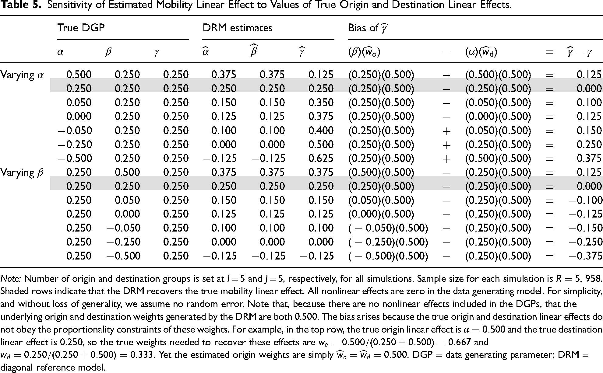
Note: Number of origin and destination groups is set at I = 5 and J = 5, respectively, for all simulations. Sample size for each simulation is $R=5,958$ . Shaded rows indicate that the DRM recovers the true mobility linear effect. All nonlinear effects are zero in the data generating model. For simplicity, and without loss of generality, we assume no random error. Note that, because there are no nonlinear effects included in the DGPs, that the underlying origin and destination weights generated by the DRM are both 0.500. The bias arises because the true origin and destination linear effects do not obey the proportionality constraints of these weights. For example, in the top row, the true origin linear effect is $\alpha =0.500$ and the true destination linear effect is 0.250, so the true weights needed to recover these effects are $w_o=0.500/(0.250+0.500)=0.667$ and $w_d=0.250/(0.250+0.500)=0.333$ . Yet the estimated origin weights are simply ${\hat{w}}_o={\hat{w}}_d=0.500$ . DGP = data generating parameter; DRM = diagonal reference model.

The bias of the DRM’s estimated mobility linear effect depends not only on the true origin and destination and linear effects, but also the underlying nonlinear effects. That is, because the bias formula depends on the DRM’s estimated weights, the estimated mobility linear effect from a DRM is in turn a function of the underlying nonlinear origin and destination effects. ¹⁷ In Appendix Table C.1, supplemental materials, we present results from simulations with various values of the nonlinear effects for origin and destination. Together, these simulations reveal that the estimated mobility effects are quite sensitive to the true values of the nonlinear origin and destination effects.

In short, DRM relies on a specific proportionality constraint to identify unique origin, destination, and mobility effects in a mobility table. Unfortunately, because the linear effects are not identified, the validity of this assumption can only be tested indirectly using the nonlinear effects. Even more problematic, regardless of the size of the underlying linear mobility effect, the DRM will set the linear effect to a very specific value. For example, as illustrated using Sobel’s (1981) fertility data, even if the mobility linear effect is extremely positive or negative, the DRM still fixes the mobility linear effect close to zero. Finally, we have provided a simple bias formula for the mobility linear effect, showing that the estimates from the DRM are sensitive to both the size and sign of the underlying origin and destination linear effects, as well as to the nonlinear effects. Taken together, these results suggest that the DRM should not be used to identify the effects of SM unless its very specific assumptions are strongly supported by sociological theory or background knowledge.

While the conventional DRM assumes fixed origin and destination weights, alternative specifications have been proposed that allow these weights to vary across the mobility table. Sobel (1985) extended the model to permit weights to differ by either origin or destination class, while Weakliem (1992) further allowed weights to vary simultaneously by both origin and destination. These extensions can accommodate more complex patterns of nonlinear effects in the data. Nevertheless, a fundamental limitation persists: due to the inherent identification problem, these extended DRM variants still impose specific constraints to identify unique linear effects of origin, destination, and mobility. In essence, all DRM formulations, regardless of their flexibility in handling nonlinearities, ultimately rely on point identification, requiring researchers to make highly specific and, as a consequence, strong assumptions about the magnitude and direction of the linear effects. Crucially, as we demonstrate in subsequent sections, the core assumptions of mobility effects models cannot be directly tested against the empirical data, making any results contingent in a nontrivial way on untestable modeling choices.

II. Generalizing Models of Mobility Effects

In this section, we show how previous generations of mobility effects models, such as the SAM and the DRM, can be understood as special cases of a bounding analysis. We first present a visualization of the identification problem at the core of mobility effects models, showing how the DRM and SAM achieve point identification by imposing extremely strong assumptions on the magnitude and direction of the linear effects. We then show how one can construct bounds on the linear effects using a variety of other constraints that generally involve much weaker assumptions. It is important to emphasize, however, that the results of any analysis of mobility effects are only as valid as the social theory or substantive knowledge used to justify the bounds.

1. Point Identification and the Canonical Solution Line

To understand how the DRM, SAM, and related models can be viewed as special cases of a bounding approach, it is crucial to recognize the geometric interpretation of the non-identifiability of the linear effects. Because mobility effects models are not fully identified, we cannot obtain point estimates for each of the origin, destination, and mobility linear effects (or effects that are partially a function of the linear effects). A convenient way to express the identification problem is to note that for any particular mobility effects model we can specify the slope as follows ¹⁸ :

$${\alpha }^{*}=\alpha +\nu ,{\beta }^{*}=\beta -\nu ,\text{and}{\gamma }^{*}=\gamma +\nu ,$$

(14)

where the asterisk ( $*$ ) indicates an arbitrary set of estimated slopes from a mobility effects model under some particular constraint and $\nu$ is a scalar fixed to some value. As equation (14) indicates, the estimated parameters are simple transformations of the true unobserved slopes $\alpha$ , $\beta$ , and $\gamma$ shifted by a single arbitrary scalar, $\nu$ . Importantly, selecting a value of the scalar $\nu$ is equivalent to specifying a particular constraint to identify a mobility effects model.

By varying values of $\nu$ (which can take on any value), we trace out what has been called the canonical solution line in a parameter space defined by the range of possible origin, destination, and mobility slopes (Fosse and Winship 2018, 2019b). It is a “solution” line because any set of possible estimates of the linear effects will lie on this line, and it is “canonical” because it is the simplest possible geometric representation of the identification problem. ¹⁹ Note that, if a mobility effects model were identified, then there would be not a line but a single point in the parameter space.

Figure 2 shows the canonical solution line based on the Sobel (1981) fertility data. ²⁰ Several crucial points are worth emphasizing regarding this figure. First, in the absence of data from a mobility table and a corresponding mobility effects model, the origin, destination, and mobility slopes may take on any combination of values in a three-dimensional parameter space. With a mobility effects model, vast areas of the parameter space can be ruled as inconsistent with the data. However, as we discuss later, this does not mean that quite strong assumptions are unnecessary for identifying unique mobility effects. Second, depending on the data, the location of the canonical solution line relative to the origin will differ, leading to different trade-offs from setting various constraints. Specifically, the location of the canonical solution line is a function of the parameters ${\mathrm{\Gamma }}_1=\alpha +\beta$ and ${\mathrm{\Gamma }}_2=\gamma +\beta$ . With Sobel’s fertility data, as noted above, these values are $\widehat{{\mathrm{\Gamma }}_1}=-0.317$ , and ${\hat{\mathrm{\Gamma }}}_2=-0.213$ . Note that these parameters are identified (as well as their difference) because the scalar $\nu$ in equation (14) cancels out. For example, ${\alpha }^{*}+{\beta }^{*}=\alpha +\nu +\beta -\nu ={\mathrm{\Gamma }}_1$ . ²¹ Finally, because the canonical solution line is a function of just two parameters ( ${\mathrm{\Gamma }}_1$ and ${\mathrm{\Gamma }}_2$ ), we can reduce our three-dimensional representation to just two dimensions. One way of doing this is by having the horizontal axis represent the destination slope, the left vertical axis the origin slope, and the right vertical axis the mobility slope (see Fosse and Winship 2018).

Figure 2.

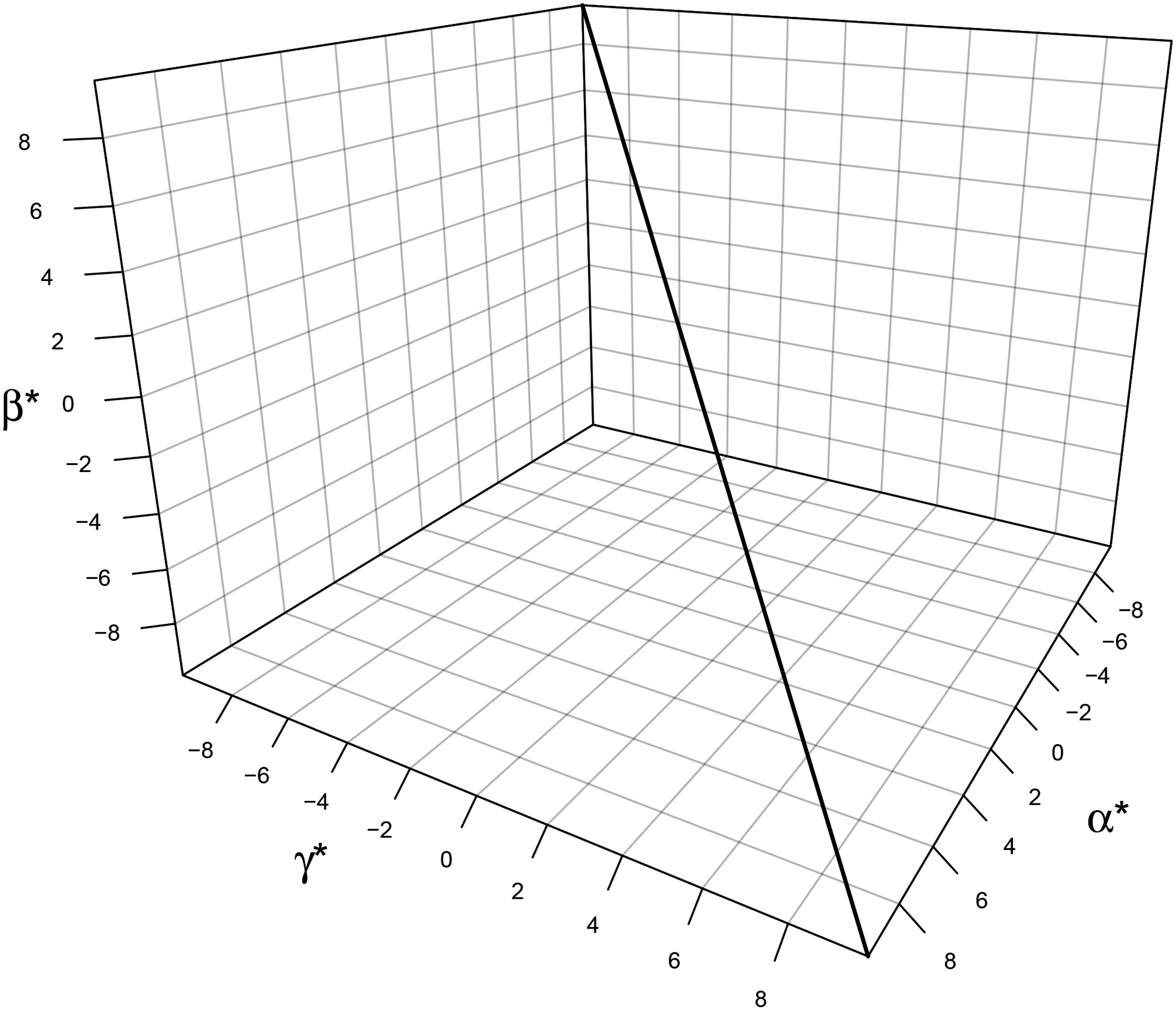
Three-dimensional (3D) canonical solution line. Note: This graph shows the canonical solution line based on Sobel’s (1981) fertility data. All possible combinations of origin, destination, and mobility slopes, denoted by ${\alpha }^{*}$ , ${\beta }^{*}$ , and ${\gamma }^{*}$ , respectively, lie on this line. Algebraically, the line is equivalent to the set of equations ${\alpha }^{*}=\alpha +\nu$ , ${\beta }^{*}=\beta -\nu$ , ${\gamma }^{*}=\gamma +\nu$ , where $\alpha$ , $\beta$ , and $\gamma$ are the true origin, destination, and mobility slopes and $\nu$ is some scalar. Any given constrained model is equivalent to selecting a particular value of $\nu$ .

Figure 3.

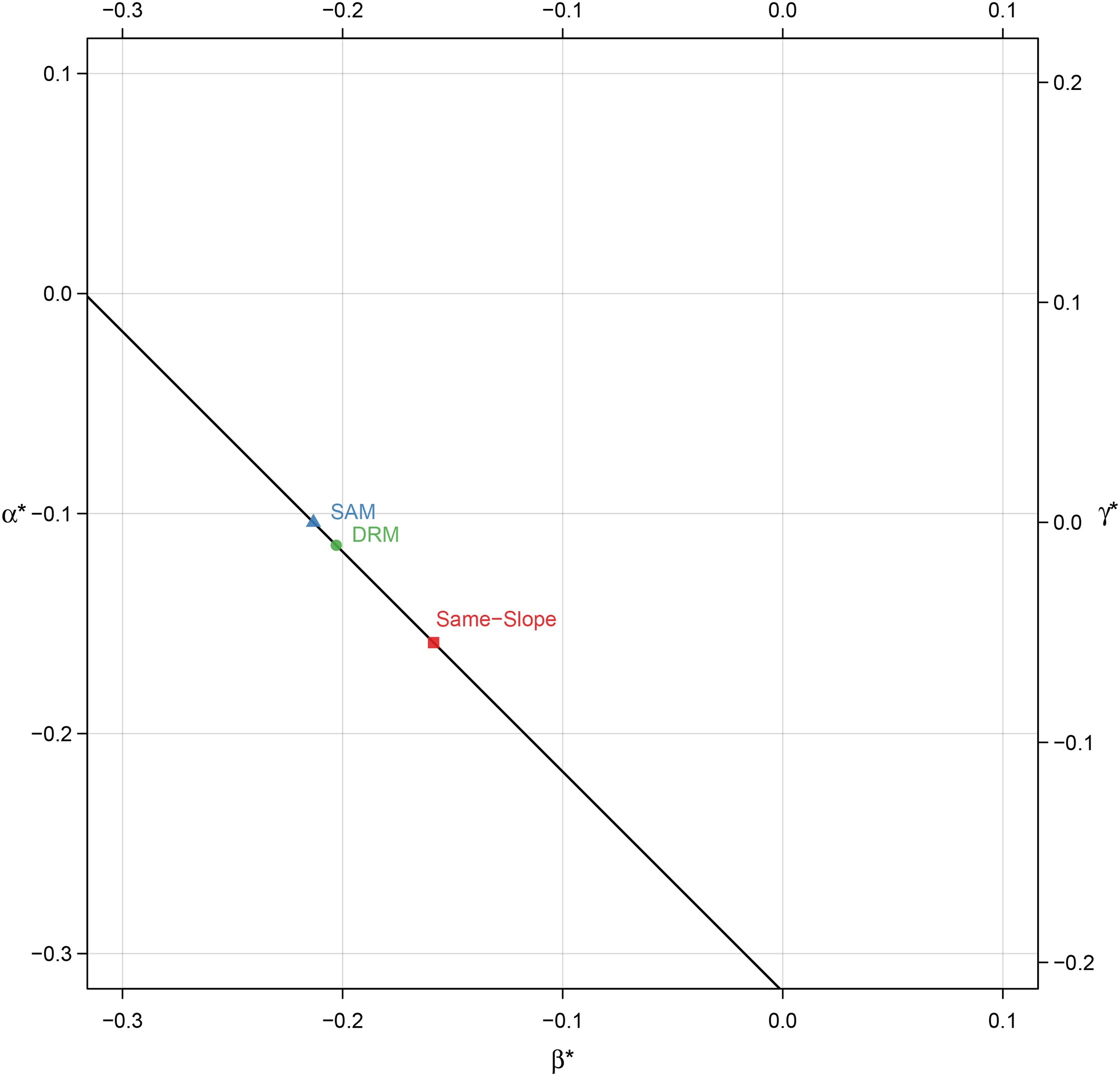
Point identification of mobility effects models: 2D canonical solution line. Note: This graph shows the 2D canonical solution line based on Sobel’s (1981) fertility data. Solution line is identical to that shown in Figure 2, but flattened to two dimensions. Points indicate estimated linear effects for the SAM, DRM, and under the assumption that origin and destination have the same slope (same-slopes). 2D = two-dimensional; SAM = square additive model; DRM = diagonal reference model.

Figure 3 shows a two-dimensional representation of the canonical solution line shown in Figure 2, again using Sobel (1981) fertility data. As in Figure 2, this line is based on values of ${\hat{\mathrm{\Gamma }}}_1=-0.317$ and ${\hat{\mathrm{\Gamma }}}_2=-0.213$ . It is important to note that the solution line shown in Figure 3 is identical to the one shown in Figure 2. Each location in the coordinate space can be referenced in terms of the origin, destination, and mobility linear effects, so that, for example, the point $(-0.167,-0.150,-0.063)$ refers to $\alpha =-0.167$ , $\beta =-0.150$ , and $\gamma =-0.063$ . ²² The solution line will always run from top left to bottom right, and the slope of the solution line relating destination to origin and mobility will always be $-1$ . Not all features of the solution line, however, are invariant. As noted above, the values of ${\mathrm{\Gamma }}_1$ and ${\mathrm{\Gamma }}_2$ determine two crucial features of the canonical solution line. First, the difference between ${\mathrm{\Gamma }}_2$ and ${\mathrm{\Gamma }}_1$ , estimated to be 0.104 in Figure 3, determines the offset between the origin and mobility scales. Thus, in Figure 3, when $\gamma =0$ , $\alpha =-0.104$ . Second, at the point, where $\beta =0$ , ${\mathrm{\Gamma }}_1$ , and ${\mathrm{\Gamma }}_2$ , respectively, determine the location of the canonical solution line with respect to $\alpha$ and $\gamma$ . Various traditional mobility effects models can be located on the solution line in Figure 2, and can be understood as making very specific assumptions about the underlying origin, destination, and mobility linear effects.

Three estimates are displayed in Figure 3. First, as shown by the triangle in Figure 3, there is the set of estimates corresponding to Duncan’s SAM. As noted previously, the SAM’s estimates are equivalent to assuming that the mobility linear effect is zero (i.e., $\gamma =0$ ). ²³ Second, there are the estimates for the DRM, as shown by the circle in Figure 3. As noted previously, assuming that the nonlinear effects satisfy the proportionality constraint, the mobility linear effect is fixed to $({\mathrm{\Gamma }}_2-{\mathrm{\Gamma }}_1)+{\mathrm{\Gamma }}_1{w}_o$ or, equivalently, $\gamma ={\mathrm{\Gamma }}_2-{\mathrm{\Gamma }}_1{w}_d$ , where again $w_o$ and $w_d$ are the origin and destination weights, respectively, with $w_d=1-w_o$ . In the case of Sobel’s fertility data, assuming the proportionality constraint is valid for the nonlinear effects, then the DRM will fix the mobility linear effect to $-0.010$ (see Table 4). ²⁴

The DRM and the SAM have traditionally been the most popular ways of point identifying mobility effects, but these are not the only options. Making any assumption about the sign and size of one of the three linear effects is sufficient to point identify the remaining two linear effects. Thus, for example, one might assume that the origin linear effect is zero, or that the destination linear effect is some specific negative value. One particularly attractive approach is to use what we call the same-slopes assumption. Presumably, origin and destination effects reflect similar, if not identical, underlying causal processes. Accordingly, in some contexts it might be reasonable, at least as a first pass, to assume that the origin and destination linear effects are the same, such that they have the same direction and magnitude. In other words, we might assume that origin and destination linear effects are the same such that $\alpha =\beta$ . This will then provide an estimate of the underlying linear mobility effect, or $\gamma$ . This constraint is easily derived from the data. Because ${\mathrm{\Gamma }}_1=\alpha +\beta$ is identified, under the same slopes assumption we know that $\alpha ={\mathrm{\Gamma }}_1/2$ and $\beta ={\mathrm{\Gamma }}_1/2$ . We also know that ${\mathrm{\Gamma }}_2=\gamma +\beta$ , so plugging in for $\beta ={\mathrm{\Gamma }}_1/2$ and rearranging terms we have $\hat{\gamma }={\mathrm{\Gamma }}_2-{\mathrm{\Gamma }}_1/2$ . This is the mobility linear effect under the same-slope assumption. Figure 3 shows the point estimates under the same-slope assumption as a square. Under the same-slopes assumption, the parameter ${\mathrm{\Gamma }}_1$ is split equally between origin and destination. With Sobel’s fertility data, ${\hat{\mathrm{\Gamma }}}_1=-0.317$ , and ${\hat{\mathrm{\Gamma }}}_2=-0.213$ . Thus, given the same-slopes assumption, we have $\hat{\alpha }=-0.159$ and $\hat{\beta }=-0.159$ and, accordingly, $\hat{\gamma }=-0.055$ .

Each of these three estimates of the mobility linear effects correspond to different patterns of overall mobility effects, which incorporate the nonlinearities. Figure 4 shows the estimated mobility effects using the three identification strategies discussed above. The main conclusion is that both the DRM and the SAM, as indicated by the appropriate lines in Figure 4, are broadly consistent with no meaningful pattern of mobility effects, apart from the up-and-down pattern of the nonlinear effects. By contrast, the assumption of equal origin and destination slopes yields an overall negative effect of SM on fertility, as indicated by the appropriate line in Figure 4. That is, upward (or downward) SM causes households to have fewer (or more) children.

Figure 4.

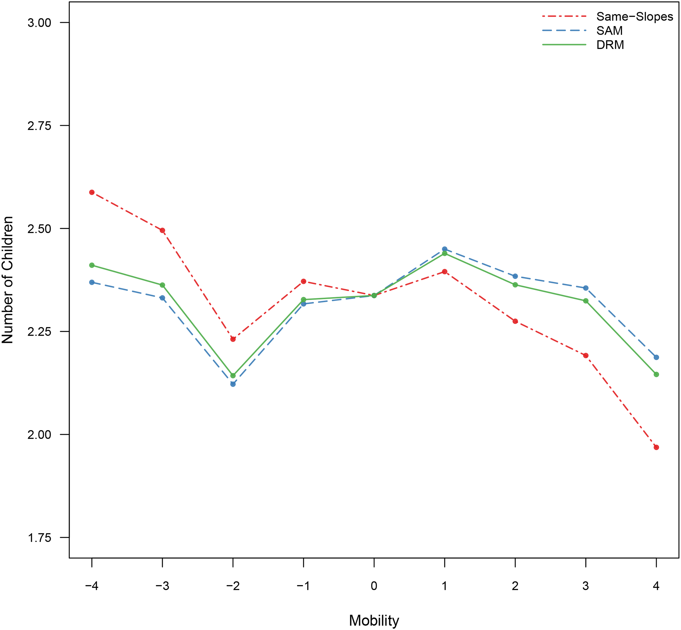
Point identification of mobility effects models. Note: This graph shows the mobility effects for the SAM, DRM, and under the same-slopes assumption for origin and destination (same-slopes). Data are based on Sobel (1981). SAM = square additive model; DRM = diagonal reference model.

The results in Figure 4 are compelling, but great caution is warranted. Only the nonlinear effects in Figure 4 are identified, while the linear effects are a function of the particular model employed, which encodes very specific assumptions about the size and sign of the linear effects. Because there is an infinite number of possible linear effects that are consistent with the data, there is also an infinite number of possible results that could be derived by applying any of a variety of mobility effects models (including those that have not yet been devised). For example, constructing a model that assumes that the origin linear effect is very negative will result in a very negative mobility linear effect, and thus a steep downward pattern in Figure 4. Conversely, using a model that assumes the origin linear effect is positive will result in a very positive mobility linear effect and, accordingly, a steep upward pattern in Figure 4. The extreme sensitivity of mobility effects models to the underlying identifying constraints used has not been generally appreciated in the literature. It should also be emphasized that the conventional mobility effects models rely on point identification, which requires invoking very specific and extremely strong assumptions that are not directly testable against the data. In the next section, we outline a number of identification strategies that involve weaker assumptions, albeit at the potential expense of the precision of the estimates.

2. Partial Identification With Bounding Analyses

Conventional models of mobility effects, as outlined above, are based on point identification, where the true parameter is uniquely estimated from the data given the specification of a particular model. Unfortunately, in the case of mobility effects, point identification depends crucially on the model (or, equivalently, on assumptions about the linear effects). As we have shown, different models (or different assumptions) lead to different estimates of mobility effects. A more principled approach is to abandon point identification in favor of partial identification. Rather than trying to extract a single estimate of a linear mobility effect, one uses (potentially weaker) assumptions to generate a range of estimates, thus partially identifying (or bounding) the mobility effect.

In the case of point identification, fixing the values of one of the slopes determines the values of the other two. For example, assuming that the mobility linear effect is zero, as is the case with the SAM, will fix the values of the origin and destination linear effects. In a similar way, setting upper and lower bounds on the magnitude and direction of any one of the linear effects will automatically set bounds on the size and sign of the remaining two linear effects. Likewise, setting the sign of any two linear effects will establish bounds on the size and sign of the remaining linear effect. ²⁵ These strategies for specifying bounds are based only on assumptions about the magnitude and direction of the underlying linear effects. However, a third strategy, which may entail even weaker assumptions, is to use the nonlinear effects to make assumptions about the shape of one or more of the effects over a particular range of the data. For example, one might assume that the pattern of destination effects is monotonically decreasing, increasing, or neither decreasing nor increasing for some (possibly restricted) set of destination categories. These assumptions will, in turn, place constraints on the underlying linear effects. ²⁶ Crucially, as Manski (1990, 2003) pointed out in his seminal work on partial identification, there is a direct trade-off between the strength of one’s assumptions and the width of the bounds on the parameters. While, in some applications, analysts may bemoan the width of the bounds to be too large to be analytically useful, wide bounds merely demonstrate that much stronger theoretical assumptions are required if the analyst seeks to usefully interpret a given estimate.

To illustrate how one might proceed with a bounding analysis of mobility effects, we outline three main partial identification strategies. First, there is what we call the same-sign assumption. Rather than assuming that the origin and destination linear effects have the same magnitude and direction, as with the same-slopes assumption, in some settings it might be appealing to assume that the origin and destination linear effects have the same sign but not necessarily the same magnitude. The justification for this assumption is again that the causal processes proxied by class origin and destination are similar, if not identical.

The constraints implied by the same-sign assumption are easily calculated from the data. Because ${\mathrm{\Gamma }}_1=\alpha +\beta$ is identified, under this assumption we know that $\alpha$ and $\beta$ each range from 0to ${\mathrm{\Gamma }}_1$ . We also know that ${\mathrm{\Gamma }}_2=\gamma +\beta$ , so plugging in for $\beta =0$ and $\beta ={\mathrm{\Gamma }}_1$ we have $\hat{\gamma }=({\mathrm{\Gamma }}_2-{\mathrm{\Gamma }}_1,{\mathrm{\Gamma }}_2)$ . In the case of Sobel’s fertility data, the same-sign assumption results in bounds of $\hat{\alpha }=(-0.317,0)$ , $\hat{\beta }=(-0.317,0)$ , and $\hat{\gamma }=(-0.213,0.104)$ . These bounds and the resultant set of estimates on the canonical solution line are shown in Panel (a) of Figure 5. The horizontal rectangle indicates the range of estimates compatible with the assumption about the origin slope, while the vertical rectangle denotes the set of estimates compatible with the assumption about the destination slope. Their intersection on the canonical solution line, which shows the set of estimates compatible with the data, is shown as a bold line. Unfortunately, in this particular case these bounds are not particularly informative, as the slope for the mobility linear effect may be negative, zero, or positive. This is evident in Figure 6(a), which shows the resultant overall mobility effects under the same-sign assumption,

Figure 5.

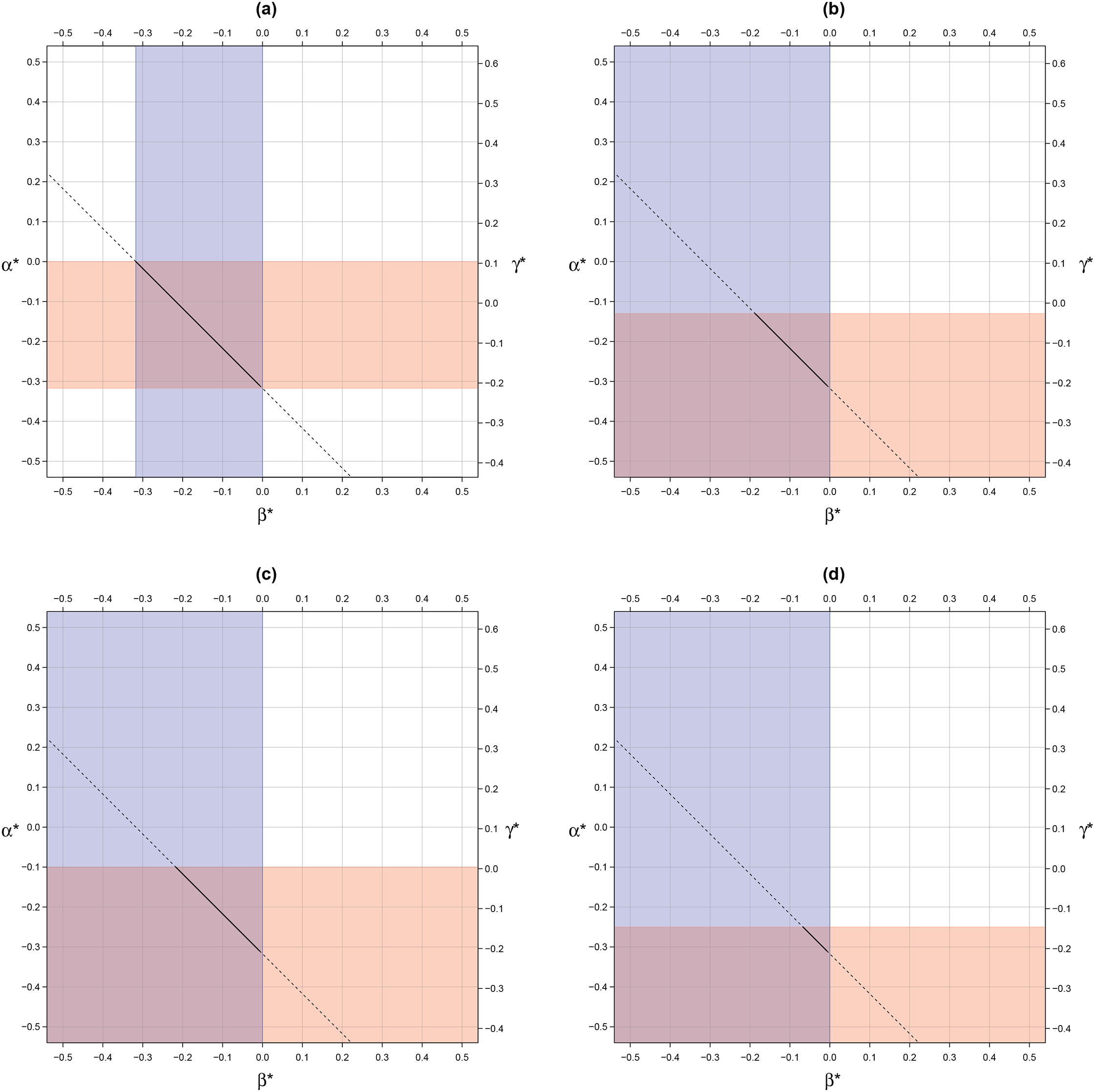
Partial identification of mobility effects models: two-dimensional (2D) canonical solution line. Note: Panel (a) shows bounds on the canonical solution line using the same-sign assumption for class origin and destination. Panel (b) shows bounds on the canonical solution line under the assumption of a monotonically downward effect for class origin (with respect to the quadratic component of the origin nonlinear effects) as well as a same-sign assumption for class destination. Panel (c) shows bounds on the canonical solution line under the assumption of a monotonically decreasing origin effect for lower-class groups (1, 2, and 3) in addition to a same-sign assumption for class destination. Lastly, Panel (d) shows bounds on the canonical solution line under the assumption of a monotonically decreasing origin effect for upper-class origin groups (3, 4, and 5) as well as a same-sign assumption for class destination. Horizontal rectangle indicates bounds on class origin while vertical rectangle denotes bounds on class destination. Bold line indicates that part of the canonical solution line consistent with the data given the particular assumptions invoked. Data are based on Sobel (1981).

Figure 6.

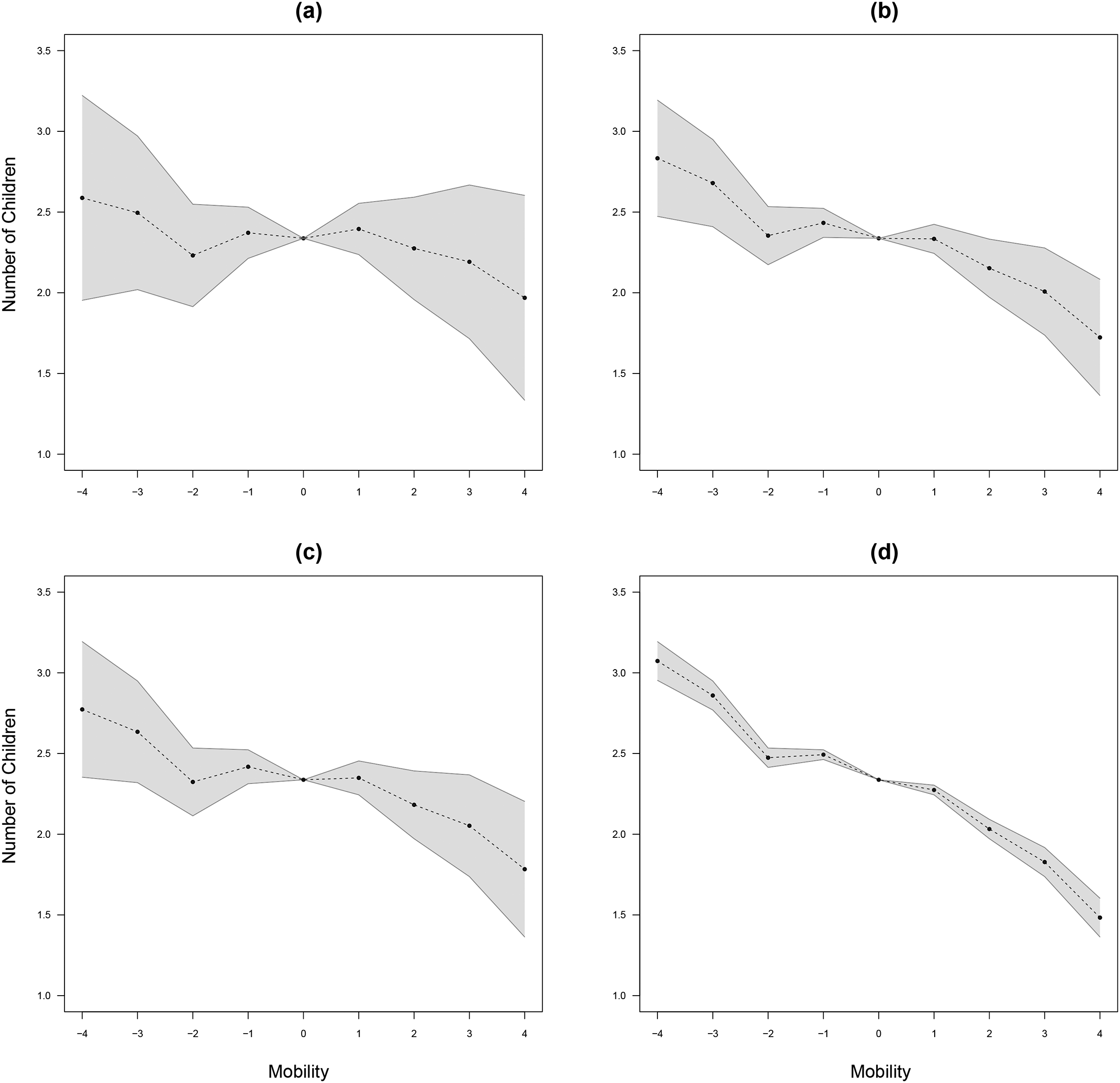
Partial identification of mobility effects models. Note: Panel (a) shows the mobility effects using the same-sign assumption for class origin and destination. Panel (b) shows bounds on the mobility effects under the assumption of a monotonically downward effect for class origin (with respect to the quadratic component of the origin nonlinear effects) as well as a same-sign assumption for class destination. Panel (c) shows bounds on the mobility effects under the assumption of a monotonically decreasing origin effect for lower-class groups (1, 2, and 3) in addition to a same-sign assumption for class destination. Lastly, Panel (d) shows bounds on the mobility effects under the assumption of a monotonically decreasing origin effect for upper-class origin groups (3, 4, and 5) as well as a same-sign assumption for class destination. Dotted line indicates the midpoint of the bounds. Data are based on Sobel (1981).

A second strategy that one might employ with mobility data is what we call the monotonic origin-destination effects assumption. The idea here is that, again to the extent that origin and destination can be understood as having similar underlying causal processes, we might assume not only that both of their linear effects have the same sign, but that one or both of the effects are monotonically increasing (if ${\mathrm{\Gamma }}_1$ is positive) or monotonically decreasing (if ${\mathrm{\Gamma }}_1$ is negative).

Some care is warranted, however, in calculating underlying linear effects based on monotonicity constraints. In many if not all cases, one might believe that the origin and destination nonlinear effects capture, at least in part, some amount of random error. Applying monotonicity constraints in such circumstances may thus be misleading. An alternative, which we use here, is to calculate the monotonicity constraints based only on some restricted set of higher-order terms, such as only the quadratic component or only the quadratic and cubic components. In other words, the effect is assumed to be monotonic only with respect to a specific subset of higher-order terms, such that the remaining nonlinear effects may themselves be monotonically decreasing, randomly fluctuating, or monotonically increasing. ²⁷ For Sobel’s fertility data, we calculate the monotonicity constraints using only the quadratic component, but substantively similar findings were obtained using higher-order terms. ²⁸

Based on the quadratic component, the maximum possible slope for a monotonically decreasing origin effect is $-0.123$ , so we specify bounds on the origin linear effect as $\hat{\alpha }=(-\mathrm{\infty },-0.123)$ . For the destination linear effect, we keep the assumption that the slope is negative, such that $\hat{\beta }=(-\mathrm{\infty },0)$ . ²⁹ Combined, these bounds result in a mobility linear effect of $\hat{\gamma }=(-0.213,-0.019)$ . The bounds for the linear effects, as well as that part of the solution line consistent with these bounds, are shown in Panel (b) of Figure 5. The overall mobility effects, which incorporate the (identified) mobility nonlinear terms, are shown in Figure 6(b). Given these assumptions, upward (or downward) mobility causes households to have many fewer (or more) children. Specifically, based on the midpoint of the bounds, those who are the most upwardly mobile ( $+4$ ) have $\sim 1.11$ fewer children than those who are the most downwardly mobile ( $-4$ ).

So far we have employed two approaches to partially identifying mobility effects, one based on the same-sign assumption and another based on monotonically decreasing origin and/or destination effects. A third approach is to invoke the assumption of monotonically decreasing effects, but to do so for some restricted range of class categories. For example, suppose we assume that fertility rates across class origin categories are monotonically decreasing, but only among those classes lower in the hierarchy (1, 2, and 3). This assumption aligns with the claim that fertility may decline consistently across individuals from lower class origins, as even modest differences in resources, education, health care, and family planning may significantly shape reproductive strategies. However, for individuals from middle class origins or higher, the primary determinants of lower fertility might be largely satisfied, resulting in stabilized fertility levels across these class groups, or at least fertility levels that are not monotonically decreasing.

The assumption that fertility is monotonically decreasing, but only across class origin categories lower in the hierarchy, results in a maximum possible origin slope of $-0.092$ . Accordingly, we specify the bounds on the origin linear effect as $\hat{\alpha }=(-\mathrm{\infty },-0.092)$ . For the destination linear effect, we again keep the assumption that the slope is negative, such that $\hat{\beta }=(-\mathrm{\infty },0)$ . Together, these bounds yield a mobility linear effect of $\hat{\gamma }=(-0.213,0.012)$ . The bounds for the linear effects, as well as that part of the solution line consistent with these bounds, are shown in Panel (c) of Figure 5, while the overall mobility effects are shown in Figure 6(c). Under these assumptions, we arrive at similar albeit more uncertain conclusions compared to those derived from Figures 5(b) and 6(b). That is, with the caveat that the mobility linear effect may be slightly positive, based on the midpoint of bounds we can conclude that those who are the most upwardly mobile ( $+4$ ) have $\sim 0.99$ fewer children than those who are the most downwardly mobile ( $-4$ ).

Alternatively, suppose we assume that fertility rates across class origin categories are monotonically decreasing, but only among those classes higher in the hierarchy (3, 4, and 5). This assumption is consistent with the claim that fertility differences are most pronounced among individuals from higher class origins, as distinctions in economic resources, aspirations, and family formation norms become increasingly influential at higher class origin positions. By contrast, among lower class origins, fertility rates may already reflect uniformly constrained resources and limited opportunities, resulting in less variation in fertility across these categories. The assumption that fertility is monotonically decreasing, but only across class origin categories higher in the hierarchy, yields a maximum possible origin slope of $-0.244$ and thus bounds on the origin linear effect of $\hat{\alpha }=(-\mathrm{\infty },-0.244)$ . As in the prior examples, for the destination linear effect we assume that the slope is negative, such that $\hat{\beta }=(-\mathrm{\infty },0)$ . These bounds together result in a mobility linear effect of $\hat{\gamma }=(-0.213,-0.141)$ . Figure 5(d) shows the bounds on the linear effects, including that section of the solution line that is consistent with these bounds. The overall mobility effects are shown in Figure 6(d), which have quite narrow lower and upper bounds. The main conclusion, largely in line with the results in Panels (b) and (c), is that upward mobility has a strong negative effect on fertility. Specifically, based on the midpoint of the bounds, we can conclude that those who are the most upwardly mobile ( $+4$ ) have about 1.59 fewer children than those who are the most downwardly mobile ( $-4$ ).

The above approaches to identifying mobility effects employ much weaker assumptions than conventional models, such as the DRM and SAM, which rely on point identification. This is not to imply that these assumptions are not very strong, however. ³⁰ In many applications, theories or additional information about the underlying causal processes may be quite ambiguous, precluding any practical guidance on how to set bounds on the effects. Moreover, even when one believes that theory or background information provides useful guidance on how to set the bounds, it is absolutely critical to understand that the results are by definition extremely sensitive to the assumptions invoked. This means that any analysis that attempts to identify unique effects of mobility is inherently provisional, and thus should always be presented transparently, clearly specifying the assumptions invoked and explicitly discussing the tentative nature of the conclusions. As we have shown, this is facilitated by parameterizing the model so that the unidentified part is separate from the unidentified part, as we have done with the L-ODM model.

Finally, it is worth underscoring that even if one believes that the true effects have been identified, there are additional and serious complications with treating such effects as “causal” in any meaningful sense. As Zang, Sobel, and Luo (2023) have recently emphasized, it is important to recognize that the DRM and related models were developed in a historical context that largely predated modern frameworks for causal inference. While these techniques represented innovative solutions to the methodological challenges of their time, they now face significant limitations when evaluated against contemporary standards for causal identification. In Appendix D, supplemental materials, we outline in detail these issues regarding parallel-world counterfactuals, the consistency assumption, the assumption of no confounding (given composite exposures), and complications that arise due to the fact that mobility is likely an exposure-induced confounder. These difficulties mean that even if the underlying bundles of mechanisms for origin, destination, and mobility could somehow be observed, there remain substantial barriers to interpreting estimated parameters as causal effects. These problems apply not only to the DRM and SAM but also to methods using bounds to partially identify effects. ³¹

III. Paradigm Shift: Towards a Positional Sociology of Social Mobility

The prior sections have critically assessed the DRM and the general challenges for the identification of independent origin, destination, and mobility effects. Taken together, we believe that the problems identified call for a fundamentally new direction in the analysis of the consequences of SM. We now begin to outline what we consider a particularly promising way forward. To be clear, this entails a re-framing of the analytic question. But, in words typically ascribed to Charles Kettering, “a problem well stated is a problem half-solved.”

The alternative framework for analyzing SM that we propose in this section is based on the concept of positional sociology (Fosse and Pfeffer 2025). This approach differentiates between two distinct forms of inequality: (1) structural inequalities, associated with stable positions within the social hierarchy, and (2) dynamic inequalities, arising from movements between social positions. Building on this distinction, we introduce the SDI model, which extends the L-ODM model by explicitly re-indexing parameters according to social origin and mobility status. The result is a fully identified model with clearly interpretable parameters that effectively capture both types of inequality. As we go on to show, this method enables a decomposition of population-level variation within mobility tables, leading to highly informative sets of parametric expressions and visualizations.

Our approach broadly aligns with recent contributions by Zang, Sobel, and Luo (2023) and Breen and Ermisch (2024). Like us, these authors emphasize challenges in isolating unique mobility effects and suggest alternative conceptualizations of SM. Specifically, they conceptualize class destinations as “treatments” whose effects vary across origin categories. However, we adopt a model that, while fully identified, nonetheless leverages the distinct, identifiable components of origin, destination, and mobility. Furthermore, and more importantly, our framework diverges from their approach by explicitly emphasizing mobility as a positional dimension rather than as a variation in destination treatment effects. Consequently, our primary objective is to use the SDI model to systematically dissect mobility tables into their constituent structural and dynamic inequalities, thereby highlighting the inequalities experienced by distinct social groups. ³²

1. Mobility as a Metric of Positionality

In contrast to conventional models of mobility effects, what we term “positional sociology” takes a distinctly different approach to the deterministic relationship between origin, destination, and mobility (Fosse and Pfeffer 2025). Whereas conventional models regard this relationship as an obstacle to be overcome, positional sociology embraces it as a natural observational fact, recognizing that origin, destination, and mobility are interrelated dimensions that locate positions in an observed social space, rather than as proxies for distinct bundles of causal mechanisms that must be separated. Positional variables are not themselves causal, but are axes along which variation is observed. Treating them as causal in and of themselves is a fundamental “category mistake” (e.g., see Ryle 1959).

Suppose, for example, that an individual from a given class origin group moves up the social hierarchy and reaches a new class destination. Reaching this new position in the social structure (ST) is observed conjointly with the degree of SM. From this perspective, SM as a dimension of positionality can never be completely separated from class destination, nor should it be, because SM is experienced in the context of class destination rather than independently of it. ³³ However, treating origin, destination, and mobility as dimensions of social position rather than as surrogates for underlying causal factors does not mean that positional sociology does not involve the study of causal processes; far from it. Rather, the causal factors are distinct and separate from the dimensions of social position, which describe the observed locations of individuals and other groups in an observed multidimensional social space. ³⁴

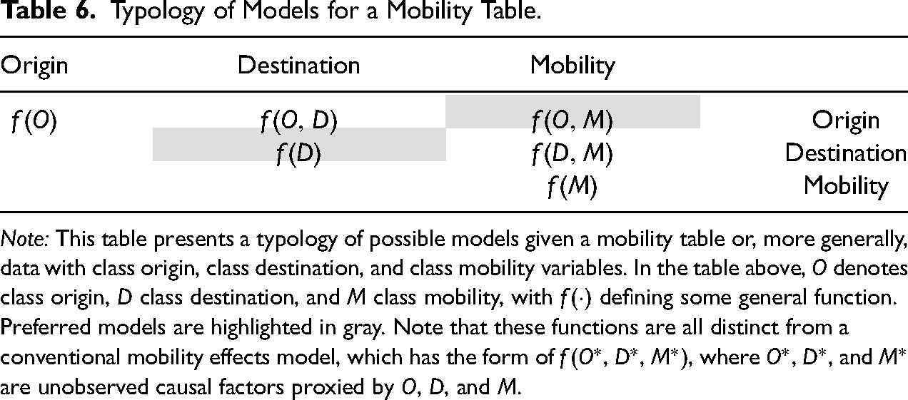
Given this epistemology, a key question is: how exactly should we describe population-level variability using information from a mobility table? There are six logically possible ways, as shown in Table 6. Let $f(.)$ denote some generic function and, as before, let O, D, and M denote the observed origin, destination, and mobility dimensions on a mobility table. We can then describe variability with models of the form $f(O)$ , $f(D)$ , $f(M)$ , or with models of the form $f(O,D)$ , $f(O,M)$ , $f(D,M)$ . For example, researchers often describe differences by class destination (e.g., Goldthorpe 1999), which corresponds to a function of the form $f(D)$ . Duncan’s SAM can be re-interpreted as a model that does not attempt to extract unique origin, destination, and mobility effects, but rather as an $f(O,D)$ model that attempts to describe the surface of a mobility table (see also Appendix E, supplemental materials).

Table 6.

Typology of Models for a Mobility Table.

Origin	Destination	Mobility
$f(O)$	$f(O,D)$	$f(O,M)$	Origin
	$f(D)$	$f(D,M)$	Destination
		$f(M)$	Mobility

Note: This table presents a typology of possible models given a mobility table or, more generally, data with class origin, class destination, and class mobility variables. In the table above, O denotes class origin, D class destination, and M class mobility, with $f(\cdot )$ defining some general function. Preferred models are highlighted in gray. Note that these functions are all distinct from a conventional mobility effects model, which has the form of $f(O^{*}$ , $D^{*}$ , $M^{*})$ , where $O^{*}$ , $D^{*}$ , and $M^{*}$ are unobserved causal factors proxied by O, D, and M.

Among these various generic models for summarizing population-level variability in a mobility table, we have a strong preference for models of the form $f(D)$ and $f(O,M)$ , which are shaded gray in Table 6. The reason is that models based on the other functions, although quite common, readily conflate structural with dynamic inequalities and thus fail to distinguish ST, or the “map of locations,” from SM, or “movements from one location to another” (Fosse 2023). ³⁵ We elaborate this view below. We also refer the reader to Appendix E, supplemental materials, which contains detailed mathematical formulas outlining the limitations of the other models shown in Table 6.

Consider first a model of the form $Y=f(O,M)+ϵ$ , where $ϵ$ is a normally distributed error term with a mean of zero. For some summary outcome Y observed in a given class destination $D=O+M$ , what we will refer to as social mobility (SM) analysis is focused on examining models of the form $Y=f(O,M)+ϵ$ . Conditional on M, variability in Y across levels of class origin O (and thus also D) reveals a ST differential, or structural inequality. This represents the “map of locations” with respect to the outcome being examined. Conversely, conditional on O, variability in Y across levels of class mobility M (and thus also D) reveals a SM gradient, or a dynamic inequality. This represents, for a given class origin, how the outcome is related to “movements from one location to another.” In summary, SM analysis as we have defined it here is concerned with distinguishing between observed differences with respect to the ST and SM, rather than with identifying unique “effects” of origin, destination, and mobility.

It is crucial to understand that SM analysis is distinct from any analysis using models of the form $Y=f(O,D)+ϵ$ or $Y=f(D,M)+ϵ$ . The reason is that conditioning on class destination conflates variations in ST with variations in SM. For example, suppose we attempt to describe a mobility table using a $f(O,D)$ function, such as Duncan’s SAM (without assuming that the estimates represent unique causal effects). Conditional on class destination (D), variations in class origin (O) will compare different origin groups with distinctly different mobility levels, producing a descriptive pattern that captures neither differences in ST nor SM, but a heterogeneous mixture of the two. ³⁶ It is only in the complete absence of SM that variations in class origin conditional on class destination will provide meaningful estimates of sociostructural differences. ³⁷

Likewise, suppose we attempt to specify a model based on a function $f(D,M)$ . Conditional on class destination (D), variations across mobility levels (M) will compare groups with distinctly different class origins and mobility levels. Importantly, these estimates will not reflect a social process that any group of individuals will ever experience, and instead conflates sociostructural differences with the SM gradient. ³⁸ Similar to the origin–destination model, the destination–mobility model will give meaningful estimates of variability with respect to SM only in the absence of sociostructural differences. ³⁹

Our approach is also distinct from one-factor models of the form $f(O)$ , $f(D)$ , and $f(M)$ . As we show in Appendix E, supplemental materials, each of these models can be understood as reflecting underlying differences in the ST as well as SM. For example, a model with just class destination is essentially differences in ST and SM, but weighted by the associations between class destination with class origin and mobility, respectively. Among these three general class of models, as noted above, our preference is for models that include just class destination. The reason is that models with just class origin or class mobility are a weighted combination of variability with respect to either ST or SM, along with a set of intra-destination differences. In contrast, a key advantage of models of the form $f(D)$ is that they provide a simple way to decompose the aggregate class destination gap into a part attributable to the ST and a part attributable to SM (see Appendix F, supplemental materials).

The injunction to use functions of the form $f(O,M)$ and $f(D)$ to examine the SDIs in a mobility table is quite general, and in principle any number of modeling approaches could be used. In the next section, we introduce a particularly useful model for conducting a SM analysis. As we show, this model parsimoniously provides a number of highly informative summaries about the nature and extent of observed differences with respect to both the ST and SM. Moreover, this model extends quite straightforwardly to more complex settings, such as those that involve multiple time points and/or continuous measures.

2. The SDI Model

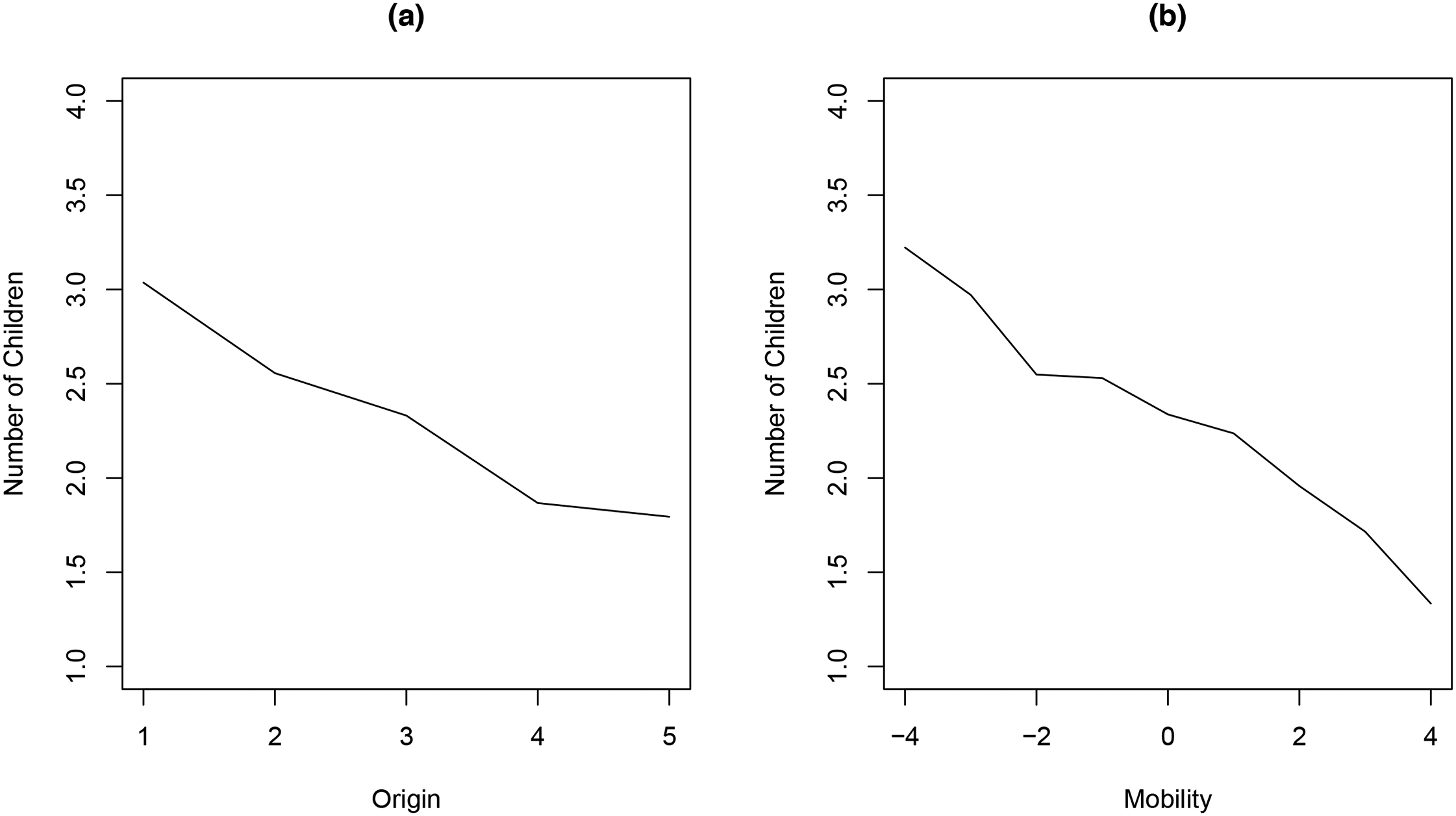
To examine differences with respect to ST and SM, we introduce what we call the structural and dynamic inequality model, or, for short, the SDI model. This model is derived by taking the L-ODM model, substituting destination with origin and mobility, and rearranging the terms. The result is a fully identified model, expressed in terms of the origin, destination, and mobility parameters, with the following general form: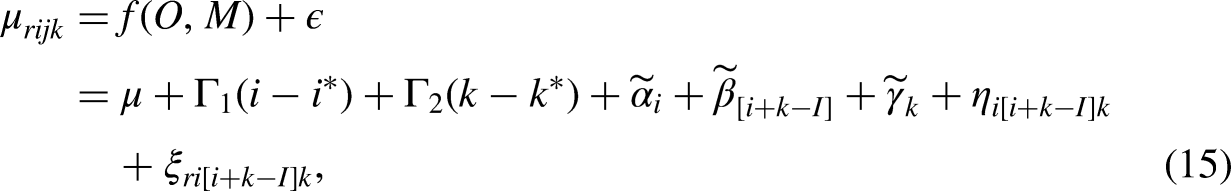

$${\mu }_{rijk}=f(O,M)+ϵ=\mu +{\mathrm{\Gamma }}_1(i-i*)+{\mathrm{\Gamma }}_2(k-k*)+{\tilde{\alpha }}_i+{\tilde{\beta }}_{[i+k-I]}+{\tilde{\gamma }}_k+{\eta }_{i[i+k-I]k}+{\xi }_{ri[i+k-I]k},$$

(15)

where the asterisks denote midpoint or referent indices $i*=(I+1)/2$ and $k*=(K+1)/2$ ; where ${\mathrm{\Gamma }}_1=\alpha +\beta$ and ${\mathrm{\Gamma }}_2=\gamma +\beta$ ; $\tilde{\alpha }$ , $\tilde{\beta }$ , and $\tilde{\gamma }$ represent the origin, destination, and mobility nonlinearities, respectively; ${\eta }_{i[i+k-I]k}$ is an additional (orthogonal) term denoting interactions; and ${\xi }_{ri[i+k-I]k}$ is a normally distributed individual-level error term with a mean of zero. Note that, by substituting the destination indices with the sum of the origin and mobility indices (i.e., $j=i+k-I$ and $J=K-I+1$ ), the outcome is only a function of class origin, indexed by i, with corresponding parameters representing differences with respect to the ST, and mobility, indexed by k, with corresponding parameters representing differences with respect to SM. Crucially, this model is identified (i.e., the design matrix is of full rank) as it does not contain a separate linear term for destination, which is instead absorbed into the linear terms indexed by origin and mobility. ⁴⁰

Somewhat remarkably, equation (15) encompasses a great deal of information about the underlying structural and dynamic inequalities in a mobility table. Accordingly, a large number of parametric expressions can be derived from the model. Among the most useful for describing the main patterns in a mobility table are those discussed and visualized in the remaining sections: the social structure matrix and social mobility matrix, the social structure slope and the social mobility slope, social structure and social mobility curves, and comparative mobility curves. In Appendix F, supplemental materials, we include a full list of expressions that can be derived from the SDI model (Appendix Table F.1, supplemental materials) and illustrate the analytic use of one additional expression (marginal class destination curve).

3. The Social Structure and Social Mobility Matrices

The SDI model allows us to decompose the overall pattern observed in a mobility table into two distinct underlying matrix-based components. This decomposition helps separate inequalities associated with social positions from those associated with movement between these positions. First, we can extract the social structure matrix. This matrix reflects the joint origin-destination parameters from the SDI model and is calculated as ${\hat{\mu }}_{ijk}=\mu +{\mathrm{\Gamma }}_1(i-i*)+{\tilde{\alpha }}_i+{\tilde{\beta }}_{[i+k-I]}$ . This matrix isolates the component of inequality related to the combination of starting position (origin) and ending position (destination), effectively representing the patterns associated purely with the ST itself. Second, we can extract the social mobility matrix. This matrix reflects the joint mobility–destination parameters from the SDI model, calculated as ${\hat{\mu }}_{ijk}=\mu +{\mathrm{\Gamma }}_2(k-k*)+{\tilde{\gamma }}_k+{\tilde{\beta }}_{[i+k-I]}$ . This matrix captures the component of inequality related to the experience of mobility (the movement itself) in conjunction with the destination reached, representing the dynamic aspect of inequality.

Figure 7 provides a visualization of these components of a mobility table using Sobel’s (1981) fertility data. Panels (a) and (b) display the overall predicted fertility values from the main parameters of the SDI model in 2D and 3D, respectively, showing the combined influence of ST and SM. Panel (c) presents the social structure matrix, illustrating how predicted fertility varies according to the joint combination of origin and destination positions, thereby highlighting structural inequalities. Panel (d) displays the social mobility matrix, showing how predicted fertility varies based on the joint combination of mobility experience and class destination, highlighting dynamic inequalities. Comparing Panels (c) and (d) visually separates the relative contributions of structural and dynamic inequalities to the overall fertility patterns. The ST matrix (Panel (c)) exhibits marked gradients, especially the trend towards lower fertility with higher origin-destination status, suggesting a prominent role for structural position. Similarly, the SM matrix (Panel (d)) illustrates significant fertility differences across various origin–mobility combinations, indicating that the dynamic component also accounts for a considerable part of the overall observed variation.

Figure 7.

Social mobility matrices. Note: Panels (a) and (b) present 2D and 3D visualizations, respectively, of the predicted mean fertility based on the SDI model’s main parameters. That is, each cell is given by ${\hat{\mu }}_{ijk}=\mu +{\mathrm{\Gamma }}_1(i-i*)+{\mathrm{\Gamma }}_2(k-k*)+{\tilde{\alpha }}_i$ $+{\tilde{\beta }}_{[i+k-I]}+{\tilde{\gamma }}_k$ . Panel (c) shows the mean fertility based on the joint origin-destination mobility parameters, such that ${\hat{\mu }}_{ijk}=\mu +{\mathrm{\Gamma }}_1(i-i*)+{\tilde{\alpha }}_i+{\tilde{\beta }}_{[i+k-I]}$ . Finally, Panel (d) shows the mean fertility based on the joint mobility-destination mobility parameters, such that ${\hat{\mu }}_{ijk}=\mu +{\mathrm{\Gamma }}_2(k-k*)+{\tilde{\gamma }}_k+{\tilde{\beta }}_{[i+k-I]}$ . Data are based on Sobel (1981). 2D = two-dimensional; 3D = three-dimensional; SDI = structural and dynamic inequality.

4. The Social Structure Slope and Social Mobility Slope

At a more fundamental level, the two linear parameters of interest in equation (15) are ${\mathrm{\Gamma }}_1$ and ${\mathrm{\Gamma }}_2$ . ⁴¹ The linear term ${\mathrm{\Gamma }}_1$ is the social structure slope, or for short, the ST slope, which describes a set of overall (linear) differences in the ST, or a structural inequality. Note that ${\mathrm{\Gamma }}_1$ is the sum of two terms from the L-ODM model: $\alpha$ , the linear origin term, and $\beta$ , the linear destination term. This is because, within a given mobility level, as we compare successive class origin groups, they are also observed in higher class destination groups. By contrast, ${\mathrm{\Gamma }}_2$ is the social mobility slope, or, for short, the SM slope, which describes a set of overall (linear) differences with respect to SM, or a dynamic inequality. Like the ST slope, ${\mathrm{\Gamma }}_2$ is the sum of two terms from the L-ODM model: $\gamma$ , the linear mobility term, and $\beta$ , the linear destination term. Again, this is because within a given class origin group, greater movement up (or down) the class hierarchy corresponds to a higher (or lower) class destination. With respect to Sobel’s (1981) fertility data, the ST slope is ${\hat{\mathrm{\Gamma }}}_1=-0.317$ , while the SM slope is ${\hat{\mathrm{\Gamma }}}_2=-0.213$ . ⁴² Both slopes are negative, indicating that higher levels in the ST as well as upward social mobility both correspond to lower levels of fertility (see also Appendix Figure G.2, supplemental materials).

The ST and SM slopes can take on different values, with different implications for the patterns observed in a mobility table (see Appendix Table G.3, supplemental materials). In a world with no SM (i.e., where the SM slope is zero), linear differences within different class destinations are the same as linear differences within different mobility groups (i.e., both will reflect the ST slope). Visually, this will appear as a set of linear differences that vary only by class origin, or across the rows of an origin–destination mobility table. Conversely, in a world with no structural inequality (i.e., the ST slope is zero), the linear differences within class origin groups will be the same as those within class destination groups (i.e., both will reflect the SM slope). Visually, this will appear as a set of linear differences that vary across mobility groups, or across the diagonals of an origin–destination mobility table. ⁴³ To our knowledge, these features of mobility tables have not been recognized before.

5. Social Structure and Social Mobility Curves

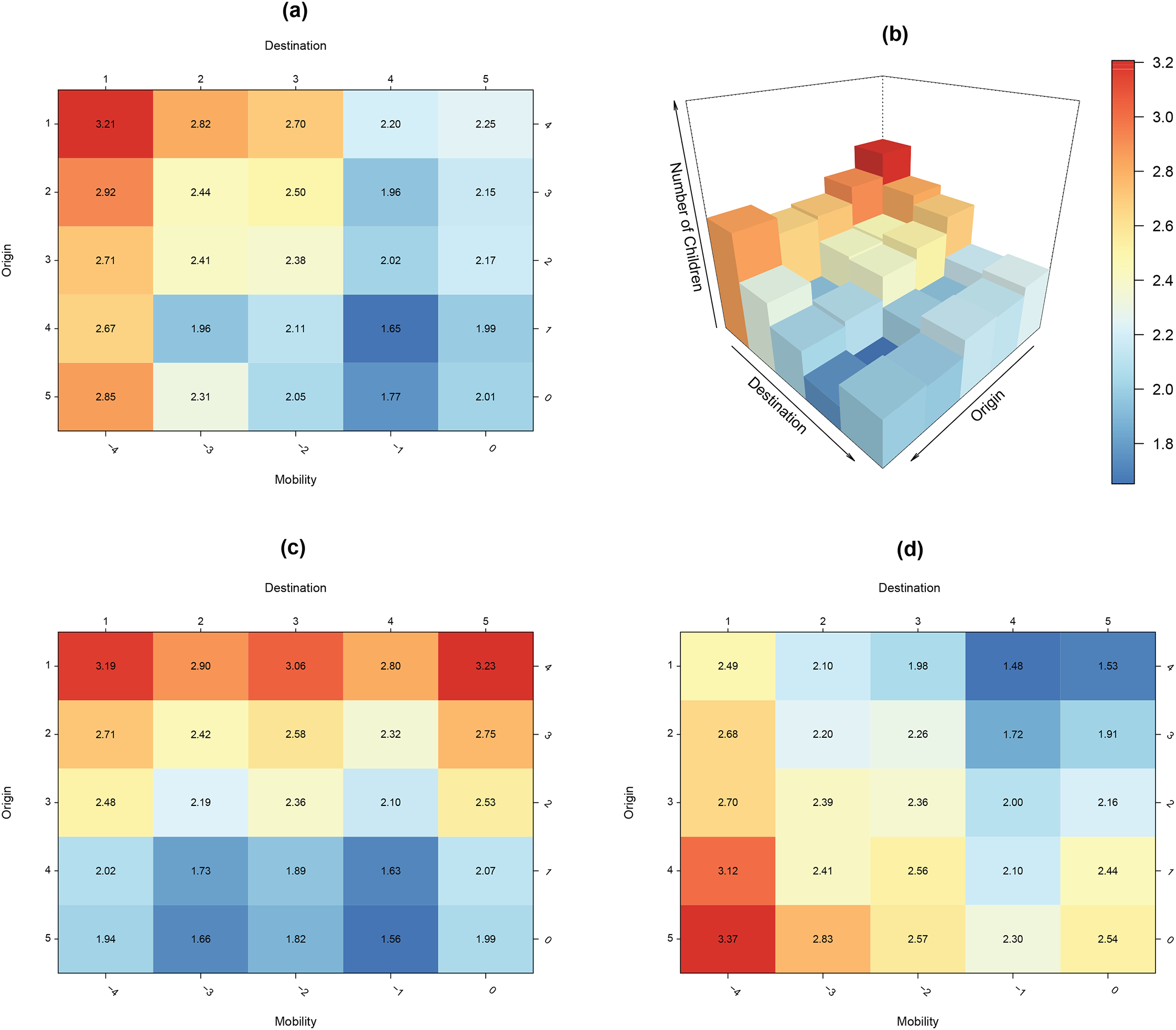
The ST and SM slopes provide basic overall information on the overall structural and dynamic inequalities observed in the data. However, more informative summaries incorporate the origin and mobility nonlinearities, respectively. Specifically, adding the origin nonlinearities along with the ST slope results in the social structure curve, or ST curve, defined by ${\mathrm{\Gamma }}_1(i-i^{*})+{\tilde{\alpha }}_i$ for origin groups $i=1,\dots ,I$ . ⁴⁴ Likewise, adding the mobility nonlinearities along with the SM slope results in the social mobility curve, or SM curve, defined by ${\mathrm{\Gamma }}_2(k-k^{*})+{\tilde{\gamma }}_k$ for mobility groups $k=1,\dots ,K$ . The ST and SM curves for Sobel’s fertility data are shown in Figure 8. Regarding structural inequality, the main conclusion is similar to that for the ST slope, with higher (or lower) positions corresponding to lower fertility levels, although with few differences between the top two social classes. Likewise, we find that upward (or downward) mobility corresponds with lower (or higher) levels of fertility.

Figure 8.

Social structure and social mobility curves. Note: Panel (a) shows the social structure (ST) curve, given by ${\mathrm{\Gamma }}_1(i-i^{*})+{\tilde{\alpha }}_i$ for class origin groups $i=1,\dots ,I$ . Panel (b) shows the social mobility (SM) curve, given by ${\mathrm{\Gamma }}_2(k-k^{*})+{\tilde{\gamma }}_k$ for mobility groups $k=1,\dots ,K$ . ${\mathrm{\Gamma }}_1=\alpha +\beta$ and ${\mathrm{\Gamma }}_2=\gamma +\beta$ . Data are based on Sobel (1981).

6. Comparative Mobility Curves

The ST and SM curves (as well as the slopes) are highly informative, compact summaries of the variability on a mobility table. However, in practice it is often useful to supplement these measures with mobility curves specific to each class origin group, or what we call comparative mobility curves. Two particularly useful versions of these curves are shown in Figure 9, again using the fertility data. First, there are what we call overall comparative mobility curves, which are defined as follows: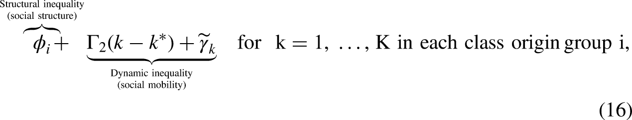

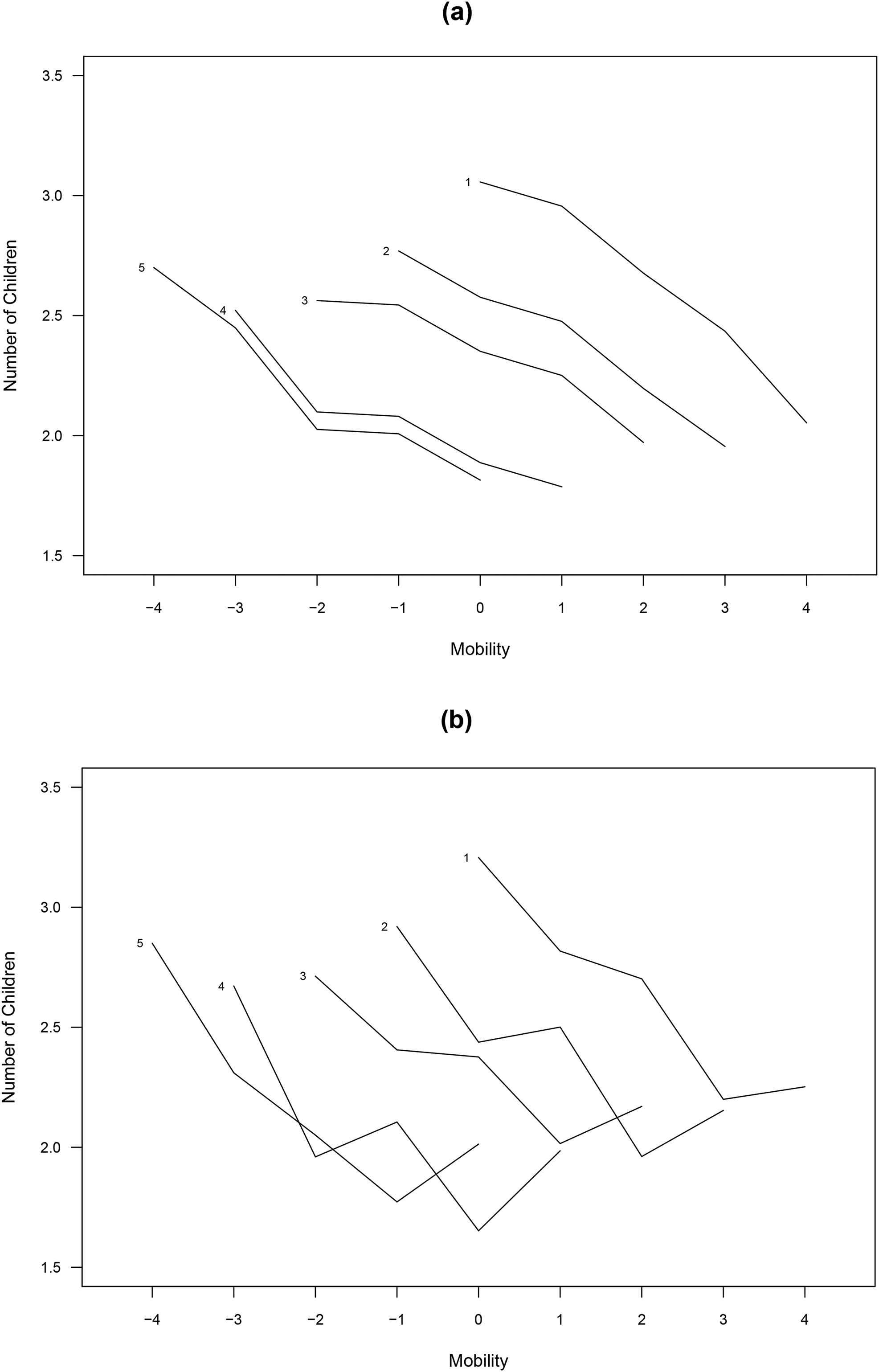
$$\stackrel{\genfrac{}{}{0ex}{}{\text{Structural ,,inequality}}{\text{( social ,,structure) }}}{\overbrace{{\varphi }_i}}+\underset{\genfrac{}{}{0ex}{}{\text{Dynamic ,,inequality}}{\text{( social ,,mobility) }}}{\underbrace{{\mathrm{\Gamma }}_2(k-k^{*})+{\tilde{\gamma }}_k}}\text{,for}k=1,\dots ,K\text{in ,,each ,,class ,,origin ,group}i,$$

(16)

where ${\varphi }_i$ acts as an intercept term, defined as ${\mathrm{\Gamma }}_1(i-i^{*})+{\tilde{\alpha }}_i$ , which takes a single, constant value for any given origin group i. This equation represents the pattern of SM for a given class origin group i in terms of the SM curve (indexed by mobility levels), or ${\mathrm{\Gamma }}_2(k-k^{*})+{\tilde{\gamma }}_k$ , and the overall structural level for a given class origin group i in terms of the ST curve (indexed by class origin), or ${\mathrm{\Gamma }}_1(i-i^{*})+{\tilde{\alpha }}_i$ .

Figure 9.

Comparative mobility curves. Note: Panel (a) illustrates the overall comparative mobility curve. Each curve represents a function of ${\varphi }_i+{\mathrm{\Gamma }}_2(k-k^{*})+{\tilde{\gamma }}_k$ for all k within a specific origin group i. In this context, ${\varphi }_i$ acts as an intercept term, defined as ${\mathrm{\Gamma }}_1(i-i^{*})+{\tilde{\alpha }}_i$ , which takes a single, constant value for any given origin group i. Panel (b) shows the adjusted comparative mobility curve. In this panel, each curve is a function of ${\varphi }_i+{\mathrm{\Gamma }}_2(k-k^{*})+{\tilde{\gamma }}_k+{\tilde{\beta }}_{i+k-I}$ for all k in each origin group i. Similar to Panel (a), ${\varphi }_i$ functions as an intercept term, calculated as ${\mathrm{\Gamma }}_1(i-i^{*})+{\tilde{\alpha }}_i$ , and maintains a single value for a given origin group i. Both panels use data based on Sobel (1981).

A slightly more complex representation is identical to equation (16) but includes the nonlinearities attributable to class destination. This results in what we call adjusted comparative mobility curves: ⁴⁵

$$\stackrel{\genfrac{}{}{0ex}{}{\text{Structural ,,inequality}}{\text{( social ,,structure) }}}{\overbrace{{\varphi }_i+{\tilde{\beta }}_{i+k-I}+}}\underset{\genfrac{}{}{0ex}{}{\text{Dynamic ,,inequality}}{\text{( social ,,mobility) }}}{\underbrace{{\mathrm{\Gamma }}_2(k-k^{*})+{\tilde{\gamma }}_k}}\text{,for}k=1,\dots ,K\text{in each class origin group}i,$$

(17)

where the ${\tilde{\beta }}_{i+k-I}$ terms are the class destination nonlinearities and, as in equation (16), ${\varphi }_i$ functions as an intercept term, calculated as ${\mathrm{\Gamma }}_1(i-i^{*})+{\tilde{\alpha }}_i$ . Note that the destination nonlinearities are indexed by both class origin and mobility levels, and thus represent both structural and dynamic inequalities.

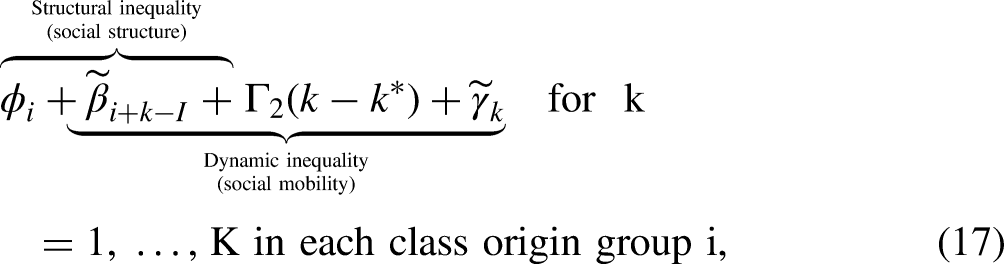
Figure 9 shows overall and adjusted comparative mobility curves using Sobel’s (1981) fertility data. Panel (a) of Figure 9 displays the collection of overall comparative mobility curves (equation (16)). Each of the class origin groups are labeled from 1 to 5. The vertical axis is the number of children, while the x-axis is the mobility dimension. Note that each class origin group is entitled to only a specific pattern of SM. For example, those at the top of the class hierarchy (Class 5) can either be immobile or move downward, while those at the bottom of the class hierarchy (Class 1) can either be immobile or move upward.

These curves encapsulate a great deal of information about the relationships between the ST and SM with respect to fertility. Vertical differences between the class origin groups are a function of the structural component, or ${\mathrm{\Gamma }}_1(i-i^{*})+{\tilde{\alpha }}_i$ . For a given origin group i, these terms effectively act like an intercept that moves the mobility curves up and down. If ST were irrelevant for fertility, then all of the mobility curves would collapse on top of each other, and thus a single mobility curve would adequately describe all of the mobility patterns. Likewise, Panel (a) of Figure 8, which shows the ST curve, would be a flat line. Horizontal differences in a given class origin group are a function of the SM component, or ${\mathrm{\Gamma }}_2(k-k^{*})+{\tilde{\gamma }}_k$ . If SM were irrelevant for fertility, then each mobility curve would be a horizontal straight line, and all differences would be described in terms of the remaining ST terms. Accordingly, Panel (b) of Figure 8, which shows the SM curve, would be a flat line.

Panel (b) of Figure 9 shows the adjusted comparative mobility curves, which are identical to the overall curves in Panel (a) except that the class destination nonlinearities are included. Vertical and horizontal differences in the graph still represent structural and dynamic inequalities, respectively, but they are now represented in a more complex way. Specifically, vertical differences between the class origin groups are now a function of ${\mathrm{\Gamma }}_1(i-i^{*})+{\tilde{\alpha }}_i+{\tilde{\beta }}_{i+k-I}$ , while horizontal differences in a given class origin group are a function ${\mathrm{\Gamma }}_2(k-k^{*})+{\tilde{\gamma }}_k+{\tilde{\beta }}_{i+k-I}$ . Note that the class destination nonlinearities, although additive in the model, are “interactive” in the data in that they appear at different mobility levels for different class origin groups (for the overall destination nonlinearities, see Appendix Figure G.1(b), supplemental materials). This is a fundamental feature of data from a mobility table that, to our knowledge, has not been previously acknowledged. What this means in practice is that a model that is additive in the parameters, such as the SDI model, can, in fact, be “interactive” in the data. ⁴⁶

Two fundamental conclusions are apparent from the mobility curves shown in Figure 9. First, conditional on SM, differences in the ST are systematically related to lower levels of fertility, particularly between Classes 1 and 2 as well as Classes 3 and 4. Second, conditional on the ST, upward (or downward) SM is systematically related to lower (or higher) levels of fertility for all class origin groups. Note that these conclusions hold even for the adjusted mobility curves shown in Panel (b), which inject additional heterogeneity into the patterns.

The results in this section underscore that there is much to be learned from a purely descriptive analysis of a simple mobility table. Rather than focusing on using information external to the data to extract unique “effects” for origin, destination, and mobility, as is common in the existing literature on mobility effects, our focus has been on estimating quantities that represent various aspects of structural and dynamic inequality. This has the great advantage of facilitating the accumulation of knowledge, as the underlying models are fully identified.

Conclusion

Despite decades of research, quantitative evidence on the consequences of social mobility has been inconclusive as it has been hampered by longstanding methodological challenges. In this article, we make a number of important contributions to the literature on social mobility effects, which has been dominated in recent years by the DRM.

We demonstrate that the DRM should not, in general, be used to identify mobility effects. Under plausible conditions, the mobility effects it estimates are biased towards zero and highly sensitive to non-intuitive and untestable assumptions, clarifying why empirical studies frequently find weak or null mobility effects. We also show that the DRM and related methods can be understood as special cases of a bounding analysis where extremely strong assumptions are invoked to achieve point identification. In this context, we provide alternative bounding strategies that not only make the assumptions more transparent but also reveal the inherently provision nature of the findings from such approaches. To address the fundamental limitations in existing methods, we conclude by introducing the structural and dynamic inequality (SDI) model, a fully identified model that relies on much weaker assumptions. As we show, the SDI model yields a large number of novel parametric expressions, and we introduce a range of graphical representations of these expressions that capture and distinguish between structural and dynamic inequalities.

An important and perhaps controversial conclusion from this article is that researchers should avoid using models that attempt to extract unique omnibus “effects” for origin, destination, and mobility. The assumptions behind these models are not only very strong but also not directly testable against the data. Of course, assumptions are fundamental to all statistical modeling, including standard approaches like ordinary least squares regression. However, we have sought to show that the necessary assumptions to identify mobility effects are much stronger than generally recognized. As a result, we consider the evidentiary basis for the individual-level effects of social mobility highly debatable. Not because this rapidly expanding literature, which overwhelmingly uses the DRM, has produced mixed and often null findings. But because using a model that is unidentified carries with it very strong, untestable assumptions, with parameters that are compatible with an infinite number of solutions. If researchers still wish to identify omnibus factors for origin, destination, and mobility, we would recommend using bounding analyses that make explicit assumptions about the size, sign, and/or shape of the effects. Ideally, these assumptions should be driven by social theory or background knowledge, and the conclusions should be stated as inherently tentative.

More importantly, however, we call for a fundamental shift in the analytic focus of mobility research. This shift rests on the basic insights that it is not meaningful to divorce social class destination from social mobility. We consider the most appropriate goal of social mobility analysis the identification of joint sets of parameters, such as the joint influence of social class destination and social mobility. We hope that this shift in focus will move the literature to more meaningful answers that can be falsified against the data. Our new approach, consistent with what we term “positional sociology,” is to treat origin, destination, and mobility as dimensions along which variability is observed, rather than as proxies for unobserved causal factors (Fosse and Pfeffer 2025). Interpreting origin, destination, and mobility as dimensions of variability, and working with functions of the form $f(O,M)$ , are the core ideas of the kind of social mobility analysis we envision.

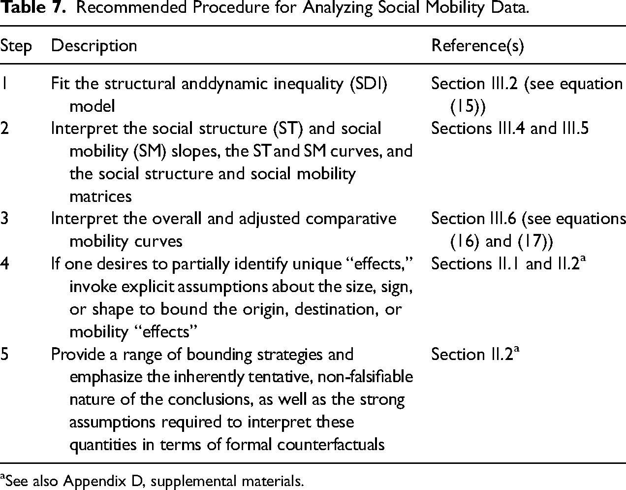
At the same time, we acknowledge that, despite the aforementioned discussion, some analysts will persist in attempting to isolate distinct “effects” for origin, destination, and mobility. To help guide applied researchers, we outline a sequence of steps for analyzing data from a social mobility table, whether one’s aim is to describe structural and dynamic inequalities based on identifiable, joint parameter sets or to extract unique effects for origin, destination, and mobility. Table 7 summarizes these steps and calls out the sections or equations in the article that match each step.

Table 7.

Recommended Procedure for Analyzing Social Mobility Data.

Step	Description	Reference(s)
1	Fit the structural anddynamic inequality (SDI) model	Section III.2 (see equation (15))
2	Interpret the social structure (ST) and social mobility (SM) slopes, the ST and SM curves, and the social structure and social mobility matrices	Sections III.4 and III.5
3	Interpret the overall and adjusted comparative mobility curves	Section III.6 (see equations (16) and (17))
4	If one desires to partially identify unique “effects,” invoke explicit assumptions about the size, sign, or shape to bound the origin, destination, or mobility “effects”	Sections II.1 and II.2a
5	Provide a range of bounding strategies and emphasize the inherently tentative, non-falsifiable nature of the conclusions, as well as the strong assumptions required to interpret these quantities in terms of formal counterfactuals	Section II.2 a

a

See also Appendix D, supplemental materials.

First, researchers should fit the SDI model, as detailed in Section III.2 and equation (15). This model serves as the foundation for understanding the distinct components of inequality. Second, the interpretation phase involves examining the social structure and social mobility slopes, the social structure and social mobility curves, as well as the social structure and social mobility matrices. These elements, discussed in Sections III.4 and III.5, provide fundamental insights into the structural and dynamic aspects of inequality. Third, a more detailed examination involves interpreting the overall and adjusted comparative mobility curves, as explained in Section III.6 and outlined in equations (16) and (17). These curves illustrate specific mobility patterns for different origin groups. Fourth, if the goal is to identify the unique “effects” of origin, destination, and mobility, then we recommend that researchers adopt a partial identification approach in which the parameters are bounded based on explicit assumptions about the size, sign, or shape of the effects. This method is covered in Sections II.1 and II.2. Finally, when employing bounding strategies, it is crucial to provide a range of these strategies and to emphasize the inherently tentative, non-falsifiable nature of the conclusions. Moreover, the strong assumptions required to interpret these quantities in terms of formal counterfactuals should be clearly articulated, as discussed in Section II.2 and Appendix D, supplemental materials.

We end by outlining a few options for future research that could extend the SDI model in a variety of different directions: first, the SDI model can be extended by interacting the components with time, allowing one to examine how the roles of social structure and social mobility change over time. Note, however, that this requires a large sample due to the sparseness at the extremes of the mobility table, as well as appropriate restrictions to deal with overfitting noise. Second, another extension is to include covariates in the model and examine potential interactions. Third, researchers should consider extending the SDI model to continuous data. This will require models that use more flexible functional forms, such as cubic regression splines or generalized additive models (GAMs), to deal with complex nonlinearities in the data. Fourth, the SDI model can be extended to address directional mobility, i.e., to distinguish the distinct patterns associated with downward and upward mobility. As currently formulated, the model captures the average linear component representing mobility-related differences (via the social mobility slope, ${\mathrm{\Gamma }}_2$ ), while accommodating asymmetric overall patterns of mobility through its flexible nonlinear mobility components. One could conceive of extensions where this linear component itself differs systematically by direction (upward vs. downward mobility). Potential modifications could involve specifying separate social mobility slopes for upward and downward mobility, possibly through interaction terms with a directional indicator or by using explicit piecewise coding. Finally, more generally, we recommend that researchers consider alternative ways of specifying models of the form $Y=f(O,M)+ϵ$ (as well as $Y=f(D)+ϵ$ ). Although we believe that the SDI model is particularly useful for summarizing data from a mobility table, other possible models, such as those that explicitly incorporate interactions between class origin and mobility, may be useful in other applications.

Supplemental Material

sj-pdf-1-smr-10.1177_00491241251358895 - Supplemental material for Beyond the Diagonal Reference Model: Critiques and New Directions in the Analysis of Mobility Effects

Supplemental material, sj-pdf-1-smr-10.1177_00491241251358895 for Beyond the Diagonal Reference Model: Critiques and New Directions in the Analysis of Mobility Effects by Ethan Fosse and Fabian T. Pfeffer in Sociological Methods & Research

Supplemental Material

sj-docx-2-smr-10.1177_00491241251358895 - Supplemental material for Beyond the Diagonal Reference Model: Critiques and New Directions in the Analysis of Mobility Effects

Supplemental material, sj-docx-2-smr-10.1177_00491241251358895 for Beyond the Diagonal Reference Model: Critiques and New Directions in the Analysis of Mobility Effects by Ethan Fosse and Fabian T. Pfeffer in Sociological Methods & Research