Sage Journals: Discover world-class research

Abstract

Many studies have compared individual measures of health expectancy across older populations by time-invariant characteristics. However, very few have included time-varying variables when calculating health expectancy. Even among older adults, socioeconomic and demographic characteristics are likely to change over the life course, and these changes may have substantial implications for health outcomes. This paper proposes a multiple multistate method (MMM) that situates the multistate model within the broader family of vector autoregressive models. Our approach allows the incorporation of the coevolution of multiple life course factors and provides a flexible yet simple way to model two or more time-varying variables with the multistate model. We demonstrate the MMM in two empirical applications, showing the flexibility of the approach to explore health expectancies with complex state spaces.

Keywords

multistate model discrete-time Markov processes microsimulation health expectancy VAR model

Introduction

In recent years, a considerable body of research has developed multistate models to explore health expectancies based on data from longitudinal sample surveys. Several main analytical approaches have been developed to estimate multistate life table quantities from longitudinal data, including the Stochastic Population Analysis for Complex Events program (Cai et al. 2010), the Interpolated Markov Chain Method (Lièvre et al. 2003), and the Gibbs Sampler for Multistate Life Tables Software (Lynch and Brown 2005). However, a shared challenge that these models face is the difficulty of handling large, complex state spaces—a shortcoming that is mostly due to the relatively small sample sizes available from longitudinal sample survey data. With some transitions represented by only a few individuals, models used to estimate transition probabilities (often logistic regression) are prone to convergence issues or may produce unreliable estimates (Allison 2008). In multistate models, including a more refined categorization of health or having more than one time-varying variable leads to a rapid growth in the size of the state space to be estimated. As this state space increases, “the number of transition schedules to be estimated increases multiplicatively” (Saito, Robine and Crimmins 2014: 216). This scaling issue leads to issues of sparsity, as observed transitions become rare and age-patterns difficult to estimate.

Due to these methodological challenges, existing studies have mostly computed health expectancy or other multistate life expectancies assuming that individual's sociodemographic characteristics remain constant over time. The literature focuses heavily on differences across time-invariant factors such as sex, race/ethnicity, and education. A few studies have explored time-varying variables such as urban/rural residence (Liu et al. 2019) and marital status (Martikainen et al. 2014) by assuming these variables remain unchanged in later life. A small body of recent studies has attempted to include time-varying variables by including them in the state space, an approach that we hereafter call the “complex multistate model (CMM).” Jia and Lubetkin (2020) combined marital and disability status into a CMM with two disability states and five different states of marital status. The resulting state space is extremely large, with many transition probabilities needing estimation. Estimating accurate transition probabilities for such a large, complex state space requires a massive amount of data, and Jia and Lubetkin (2020) used data from Medicare Health Outcomes Survey comprising over 160,000 respondents. Huang et al. (2021) computed the health expectancy of older Chinese adults combining physically active and cognitive impairment-free life in a CMM. Yet, their state space omitted some of the possible states without further explanation. Another paper by Shen and Payne (2023) developed a multidimensional extension to prior work on health expectancy by simultaneously modeling changes in morbidity and disability across a set of cohorts in the U.S. Health and Retirement Survey (HRS). However, they used a simple state space of five states (using binary measures of any vs. no morbidities and any vs. no disability) to estimate these quantities, even with the substantial sample size of the HRS.

An active strain of research on multistate methods has sought to overcome some of the limitations associated with estimating health expectancies in complex state spaces. A recent paper by Lynch and Zang (2022) used a Bayesian approach to account for issues of data sparsity when estimating quantities in CMMs. This, to some extent, could be helpful when transition events between some states are rare. However, they still experienced convergence issues due to sparsity in the transition matrix in their 10-state example. Other studies have also sought to incorporate time-varying variables using methods other than the traditional multistate model. Chiu (2019) computed the disability-free life expectancy by living arrangements in the U.S.A., claiming that living arrangement is treated as a time-varying covariate in the model. However, the description of the method is unclear about how this time-variant covariate was operationalized. Only one method—the simultaneous equation system used by Yang and Hall (2008)—appears to address this issue. This method estimates health expectancy with several time-variant covariates (i.e., body mass index, medical events, and chronic diseases) within a system of equations. Yet, little existing research has applied this method, partly due to its statistical complexity. Thus, the aim of this paper was to develop a simple and generalizable method to allow increased complexity of coevolution in multistate models, such as multiple dimensions of health, or interactions between health and socioeconomic variables, when estimating health expectancies or other multistate life expectancies.

Conceptually speaking, in multistate models, when an individual moves to a different state that individual assumes a new set of transition probabilities. A similar idea can be found in CMMs, where a change in one of the time-varying variables impacts both its own transition probabilities and the transition probabilities of the other time-varying variables. For example, an individual becoming obese shifts not only the probability of whether they will be obese in the future but also their probability of developing diabetes.

In this paper, we introduce a formulation of a CMM with more than one time-varying variable (e.g., Jia and Lubetkin 2020; Shen and Payne 2023) as a recursive vector autoregressive (VAR) model. We call this new representation of the CMM the multiple multistate method (MMM). The concept of this modeling framework shares many similarities with the VAR model popular in econometric time-series studies, which is used to capture the relationship between multiple variables as they change over time. VAR models have not been used in the context of modeling health expectancy before, although they have been applied in actuarial studies to forecast mortality (e.g., Chang and Shi 2021; Guibert, Lopez and Piette 2019; Li and Lu 2017; Li and Shi 2021). In the Method section, we describe how the MMM can exactly replicate a CMM and discuss how the flexibility of the MMM approach can reduce estimation difficulties by removing less important interactions when estimating complex state spaces.

To better illustrate our method, we apply it to two examples. The first example replicates the results in a recent paper (Shen and Payne 2023) which uses a five-state multistate model to estimate health expectancies in morbidity and disability among four successive birth cohorts in the U.S. born from 1914–1923 to 1944–1953. To demonstrate the method, we adopt the same data and compare results between the CMM and the MMM. In the second example, we explore a similar research question to Jia and Lubetkin (2020). Instead of looking at marital status and activities of daily living (ADL) disability, we select another commonly used health indicator—self-rated health (e.g., Crimmins 2004; Payne 2022). Kananen et al. (2021) suggest that self-rated health is a valid indicator of individual's overall health assessment including biological conditions. For decades, many studies have discussed the association between marital status and health. Most of them suggest a positive or protective effect of marriage on health and survival (Goldman, Korenman and Weinstein 1995; Rendall et al. 2011; Verbrugge 1979). Others also found negative effects of widowhood or divorce (Korinek et al. 2011; Verbrugge 1979). Yet, only very few studies examined the impact through the lens of multistate life expectancy until Jia and Lubetkin’s (2020) study. Thus, this example may provide dynamic insight into how marital status and health status interact as individuals’ age. At the end, we discuss that the MMM could be even more useful when modeling more than two variables with more refined categories.

Method

Complex Multistate Model

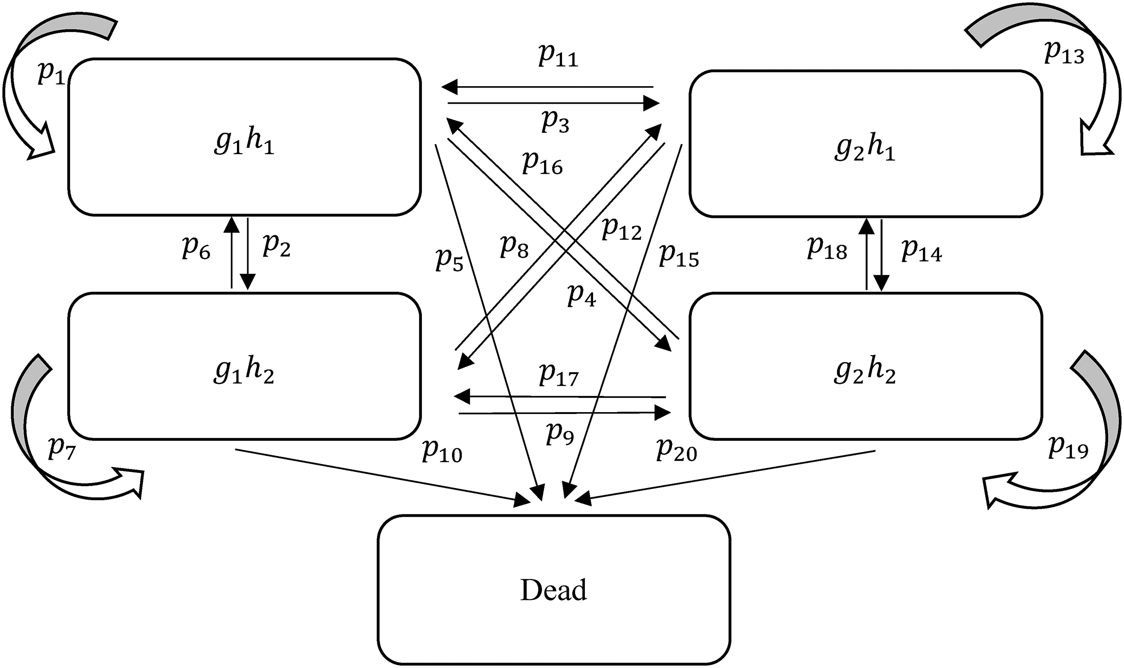
To explore the interaction between two time-varying variables with, for example, two categories each, the traditional complex multistate method would combine the two variables to form five distinct states with one absorbing state for death; the first time-varying variable G has two categories, $g_{1}$ and $g_{2}$ , and variable H has $h_{1}$ and $h_{2}$ . There are different approaches to estimate transition probabilities or rates for the expectancy (e.g., Allison 1982; Dudel 2021; Lynch and Brown 2005). The method in this paper is built on logistic regression, one of the most widely used discrete-time methods (Allison 1982; Cai et al. 2010). The state space is shown in Figure 1 and the corresponding Table 1 presents the matrix of transition probabilities within the state space, where the row names represent the current state, and the column names refer to the state in time t + 1. Each row sums up to one.

Figure 1.

Complex multistate model.

Table 1.

Transition Probabilities of the CMM in Figure 1.

Time t	Time $t + 1$
Time t	$g_{1} h_{1}$	$g_{1} h_{2}$	$g_{2} h_{1}$	$g_{2} h_{2}$	$Dead$
$g_{1} h_{1}$	$p_{1}$	$p_{2}$	$p_{3}$	$p_{4}$	$p_{5}$
$g_{1} h_{2}$	$p_{6}$	$p_{7}$	$p_{8}$	$p_{9}$	$p_{10}$
$g_{2} h_{1}$	$p_{11}$	$p_{12}$	$p_{13}$	$p_{14}$	$p_{15}$
$g_{2} h_{2}$	$p_{16}$	$p_{17}$	$p_{18}$	$p_{19}$	$p_{20}$

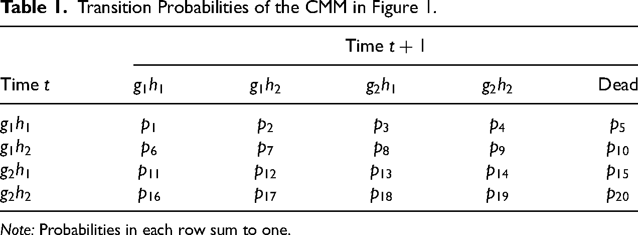
Note: Probabilities in each row sum to one.

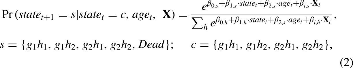
Using multinomial regression, we can estimate the transition probabilities as shown below: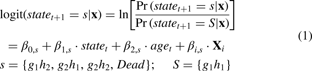

\begin{aligned} logit (s t a t e_{t + 1} = s | x) = \ln [\frac{Pr (s t a t e_{t + 1} = s | x)}{Pr (s t a t e_{t + 1} = S | x)}] \\ = β_{0, s} + β_{1, s} \cdot s t a t e_{t} + β_{2, s} \cdot a g e_{t} + β_{i, s} \cdot X_{i} \\ s = {g_{1} h_{2}, g_{2} h_{1}, g_{2} h_{2}, D e a d}; S = {g_{1} h_{1}} \end{aligned}

(1)

where

X_{i}

may include other fixed covariates, such as sex or education. Multinomial logistic regression can be understood as simultaneous estimates of a series of binary logistic models comparing each state, s, to the reference state, S (set to

g_{1} h_{1}

), given all the covariates on the right-hand side (Agresti 2007; Fullerton and Xu 2018; Long and Freese 2001). In other words, if there are K possible states, there will be

K - 1

equations that are each estimated relative to the reference state. As opposed to estimating separate binary equations, the advantages of multinomial logistic regressions are that the probabilities of each state sum to one and that we can exponentiate the coefficients to obtain ratios of probabilities (i.e., risk ratios) which are more intuitive than odds ratios from binary logit regressions. This regression model assumes, as in prior literature (e.g., Cai and Lubitz 2007; Laditka and Wolf 1998; Lim et al. 2019), that the transitions follow a discrete-time Markov chain, and the transition probabilities are age-specific. A set of coefficients is estimated for each comparison to the baseline. The predicted probability of being in state s at time t + 1 given the current state, c, and other covariates can be expressed as below:

\begin{aligned} Pr (s t a t e_{t + 1} = s | s t a t e_{t} = c, a g e_{t}, X) = \frac{e^{β_{0, s} + β_{1, s} \cdot s t a t e_{t} + β_{2, s} \cdot a g e_{t} + β_{i, s} \cdot X_{i}}}{\sum_{h} e^{β_{0, h} + β_{1, h} \cdot s t a t e_{t} + β_{2, s} \cdot a g e_{t} + β_{i, h} \cdot X_{i}}}, \\ s = {g_{1} h_{1}, g_{1} h_{2}, g_{2} h_{1}, g_{2} h_{2}, D e a d}; c = {g_{1} h_{1}, g_{1} h_{2}, g_{2} h_{1}, g_{2} h_{2}}, \end{aligned}

(2)

where

s t a t e_{t}

is a vector of dummy variables listed in the sets after equation (2) and h includes all five possible states with the coefficients (β) being 0 when s (or h) is the reference state. In other words, when s is the reference state, the probability of transitioning to state s from a given state c would be equal to one minus the sum of the probability of transitioning to the other states from that given state c. The possible values of s and c are listed in the sets after equation (2).

X_{i}

includes all the covariates other than

s t a t e_{t}

and

a g e_{t}

Apart from the transition probabilities, we also need to obtain the baseline (radix) characteristics at the starting age. One of the common methods is to use the information directly from the longitudinal survey. In cases where single age groups are small, one could combine 5–10 years around the starting age to construct a synthetic cohort (e.g., Crimmins, Hayward, and Saito 1994; Laditka et al. 2021; Payne 2022; Shen and Payne 2023). Alternatively, one could source external data such as a census or a large-scale cross-sectional dataset around the same period as the longitudinal survey to construct the baseline at the starting age (e.g., Moretti et al. 2023).

After obtaining the transition matrix and baseline, we can use microsimulation to calculate the life and health expectancies. To do this, we would generate 100,000 individuals, with their characteristics set to match the baseline population. The probabilities in each row of Table 1 are mapped into subsets in the interval of 0–1 based on the size of each probability. For example, the first row would be turned into five subsets: $[0, p_{1})$ , $[p_{1}, p_{1} + p_{2})$ , $[p_{1} + p_{2}, p_{1} + p_{2} + p_{3})$ , $[p_{1} + p_{2} + p_{3}, p_{1} + p_{2} + p_{3} + p_{4})$ , and $[p_{1} + p_{2} +$ $p_{3} + p_{4}, 1]$ . Then a random number, X, is drawn from the uniform distribution, $X \sim U (0, 1)$ . As in Laditka and Wolf (1998), the next state of the individual with a given current state and other characteristics is assigned to whichever subset this random number falls into. Life/health expectancy can also be calculated using multistate life table methods, with the same transition probabilities and baseline characteristics. However, the synthetic cohort from microsimulation can provide much richer information on individuals’ life courses, beyond simple estimates of aggregated life expectancy (Laditka and Wolf 1998).

With the basis of the traditional multistate model explained, we can introduce the MMM and highlight its distinct features. As mentioned in the Introduction, one of the challenges of the traditional multistate model lies in handling sparse transitions in a large state space. In the case of two categories within each dimension of health and five states in total, the traditional multistate model is still manageable. However, when the number of categories within variables or the number of time-varying variables increases, the observed events could become too sparse to reliably estimate transition probabilities in a regression. Additionally, building coevolving variables from very different domains of the life course into one state space may not be theoretically reasonable. The relationship between the coevolving variables cannot be easily modified according to the theory or hypothesis because it is built into the state space. To better compute life expectancy with coevolving relationships, the MMM instead models different time-varying variables separately in multiple logistic regressions.

Multiple Multistate Method

The concept of MMM shares many similarities with the VAR model, which is commonly used in macroeconomic and financial modeling to capture the relationship between multiple coevolving variables within the system as they change over time. VAR models allow for several endogenous (i.e., coevolving) variables to be estimated via a series of ordinary least squares regressions where each regression has identical covariates (Enders 2014; Greene 2000). Standard VAR models are therefore simple to estimate, and if required, the error correlation matrix can subsequently be estimated with average sums of squares or cross products of the least squares residuals (Greene 2000). In our context, this means that a VAR model can estimate a system of equations where, for example, disability can be modeled as a function of morbidity, and morbidity can be modeled as a function of disability. A VAR model usually takes one of the three forms: reduced-form VAR, recursive VAR, and structural VAR (Stock and Watson 2001). In a reduced-form VAR, each variable is modeled as a function of its own past and the past values of the other variables (i.e., the lags of the variables), but the model does not capture the contemporaneous effects (Enders 2004). On the other hand, recursive and structural VAR models include the lags of the variables similar to a reduced-form VAR, but in addition, they also allow the outcome variables in each equation to depend on the contemporaneous values of the other variables (Stock and Watson 2020).

The CMM is analogous to a structural VAR model, as the coevolving variables are estimated within one equation system. However, both reduced-form and recursive VAR models can be estimated by separate equations for each of the coevolving variables (Enders 2014; Pfaff 2008; Stock and Watson 2001). One can use recursive VAR to reverse-engineer the parameters in the structural VAR (Enders 2014). This is the basis of why our recursive MMM can replicate a CMM. On the other hand, the advantage of a reduced-form VAR compared to a recursive VAR is in its simplicity, as we can reduce the insignificant parameters in the model. However, by doing so, a reduced-form VAR cannot recover the structural VAR because of the under-identification of parameters (Enders 2014). Put it another way, a reduced-form VAR does not include the contemporaneous variables, and the short-run concurrent relationship would be ignored. Thus, a reduced-form VAR is a suitable model that the variables not directly influence each other contemporaneously, but rather any influence occurs with a time lag between the variables.

In economics, the lag length for the variables in each equation is typically estimated via F-tests or information criteria (such as the Akaike information criterion or the Bayesian information criterion). Using one lag is consistent with the common multistate assumption of a first-order Markov chain, and annual or biannual survey data collection. With the Markov assumption, the current state depends only on the previous state, which can be regarded as a univariate autoregression with lag one, VAR(1). When the state spaces are the combinations of two variables (a complex multistate), it is possible to turn this into bivariate autoregressions with lag one maintaining the Markov assumption. As aforementioned, there are various types of VAR models, and the CMM model is close to a structural VAR and the structural VAR can be estimated with a recursive VAR.

VAR models are usually estimated with continuous time-series variables such as macroeconomic and financial data, where each equation in the VAR system is estimated via ordinary least squares regressions. However, in our context, the variables are binary, and we therefore estimate the equations via logit regressions. Such “logistic VAR models” have previously been applied in empirical work (e.g., Epskam 2013; Huang et al. 2020). In the following paragraphs, we will first explain how the estimation is done and demonstrate the comparability between the CMM and the bivariate recursive MMM. Then, we will discuss the potential alternative model—the reduced-form MMM—in the Applications section.

For an MMM with a recursive term, the idea is to separately model variables H and G in sequence. One of the variables is a function of the lag of this variable (or time t), and the second variable is a function of value of time $t + 1$ and time t of the first variable, and so on. In our case with two variables, there are two options for estimation: estimating H first then G as in equations (3a) and (3b), or estimating G first then H as in equations (4a) and (4b):

logit (G_{t + 1}) = β_{0, g} + β_{1, g} G_{t} + β_{2, g} H_{t} + β_{3, g} a g e_{t} + β_{i, g} X_{i},

(3\rm a)

logit (H_{t + 1}) = β_{0, h} + β_{1, h} H_{t} + β_{2, h} G_{t} + β_{3, h} G_{t + 1} + β_{4, h} a g e_{t} + β_{i, h} X_{i},

(3\rm b)

logit (H_{t + 1}) = β_{0, h} + β_{1, h} H_{t} + β_{2, h} G_{t} + β_{3, h} a g e_{t} + β_{i, h} X_{i},

(4\rm a)

logit (G_{t + 1}) = β_{0, g} + β_{1, g} G_{t} + β_{2, g} H_{t} + β_{3, g} H_{t + 1} + β_{4, g} a g e_{t} + β_{i, g} X_{i},

(4\rm b)

where

X_{i}

includes all the covariates other than

H_{t}

H_{t + 1}

, and

G_{t}

G_{t + 1}

, and

a g e_{t}

. Note that there could be other modeling options if there are more than two variables in the system. These different options of modeling would produce different coefficients and predicted probabilities for each of the variables. For example,

β_{1, g}

in equation (3a) is not the same as

β_{1, g}

in equation (4b).

Another related issue is how to model the transition to mortality with two regressions. In the following paragraphs, we explain that mortality only needs to be modeled in one of the regressions and that both sets of equations produce the same results after joining probabilities for these variables together. A person can possess multiple time-varying characteristics at the same time, but there is only one dead state in Figure 1. If we look at these time-varying characteristics in separate models, the transition probabilities to death for the same group of individuals should be equivalent because the number of transitions to death are the same from any time-varying characteristic. Since the probabilities of death are theoretically equivalent, death can be modeled alongside any of the time-varying variables when the contemporaneous term in equation (3b) (i.e., $G_{t + 1}$ ) or equation (4b) (i.e., $H_{t + 1}$ ) is not among the independent variables. However, in this recursive example, the transition of mortality should always be modeled with the regression without the recursive term (i.e., equation (3a) or (4a)) because both variables H and G should be either dead or alive at the same time (t or $t + 1$ ). Thus, Figure 2(a) illustrates the state space for equations (3a) and (3b) where transition to death is modeled with variable G, whereas in Figure 2(b) transition to death is only modeled with variable H as in equations (4a) and (4b).

Figure 2.

(a) Multiple multistate method with bivariate recursive VAR(1), equations (3a) and (3b). (b) Multiple multistate method with bivariate recursive VAR(1), equations (4a) and (4b).

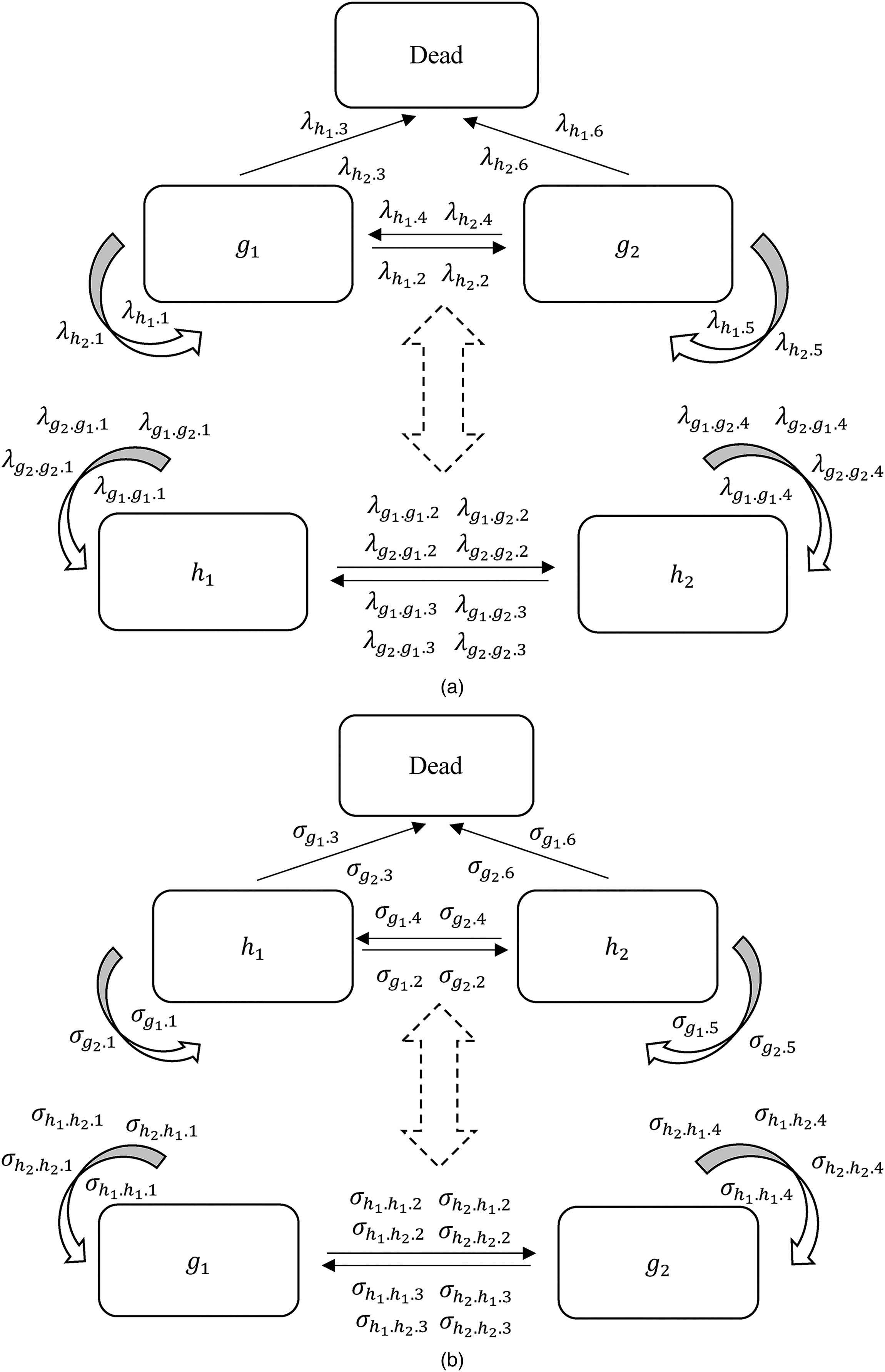
Tables 2a and 2b show the corresponding transition matrices for each option of the model. Both tables have two panels. Panel i represents the transitions in the upper model (i.e., equation (3a) or (4a)) and panel ii the lower one (i.e., equation (3b) or (4b)). Each row should also sum to one. The row names in Tables 2a and 2b represent the current state of the time-varying variable that is modeled, and the state at time t (and $t + 1$ ) of the other time-varying variable is in a subscript. For example, in Table 2a, panel i, $g_{1 h_{t} = h_{1}}$ represents the individuals that are in states $g_{1}$ and $h_{1}$ at time t, and $λ_{h_{1} .1}$ represents the probability that these individuals transition to state $g_{1}$ at time $t + 1$ . As for panel ii in Table 2a, $h_{1 g_{t} = g_{1}, g_{t + 1} = g_{1}}$ represents the individuals that are in states $g_{1}$ and $h_{1}$ at time t and transition to state $g_{1}$ at time $t + 1$ , and $λ_{g_{1} . g_{1} .1}$ is their probability to transition to state $h_{1}$ .

Table 2a.

Transition Probabilities of the MMM in Figure 2(a).

i. Transition Matrix for Variable G
Time t	Time $t + 1$
Time t	$g_{1}$	$g_{2}$	$Dead$
$g_{1 h_{1}}$	$λ_{h_{1} .1}$	$λ_{h_{1} .2}$	$λ_{h_{1} .3}$
$g_{2 h_{1}}$	$λ_{h_{1} .4}$	$λ_{h_{1} .5}$	$λ_{h_{1} .6}$
$g_{1 h_{2}}$	$λ_{h_{2} .1}$	$λ_{h_{2} .2}$	$λ_{h_{2} .3}$
$g_{2 h_{2}}$	$λ_{h_{2} .4}$	$λ_{h_{2} .5}$	$λ_{h_{2} .6}$

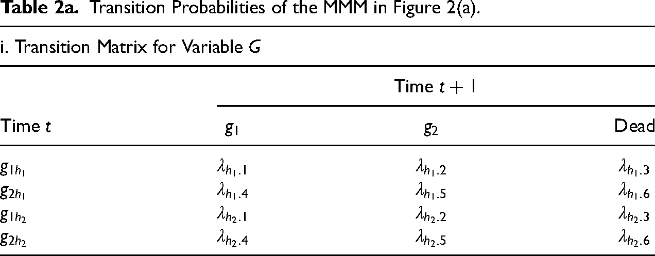
ii. Transition Matrix for Variable H

Time t	Time $t + 1$
Time t	$h_{1}$	$h_{2}$
$h_{1 g_{1}, g_{1}}$	$λ_{g_{1} . g_{1} .1}$	$λ_{g_{1} . g_{1} .2}$
$h_{2 g_{1}, g_{1}}$	$λ_{g_{1} . g_{1} .3}$	$λ_{g_{1} . g_{1} .4}$
$h_{1 g_{1}, g_{2}}$	$λ_{g_{1} . g_{2} .1}$	$λ_{g_{1} . g_{2} .2}$
$h_{2 g_{1}, g_{2}}$	$λ_{g_{1} . g_{2} .3}$	$λ_{g_{1} . g_{2} .4}$
$h_{1 g_{2}, g_{1}}$	$λ_{g_{2} . g_{1} .1}$	$λ_{g_{2} . g_{1} .2}$
$h_{2 g_{2}, g_{1}}$	$λ_{g_{2} . g_{1} .3}$	$λ_{g_{2} . g_{1} .4}$
$h_{1 g_{2}, g_{2}}$	$λ_{g_{2} . g_{2} .1}$	$λ_{g_{2} . g_{2} .2}$
$h_{2 g_{2}, g_{2}}$	$λ_{g_{2} . g_{2} .3}$	$λ_{g_{2} . g_{2} .4}$

Note: Probabilities in each row sum to one.

Table 2b.

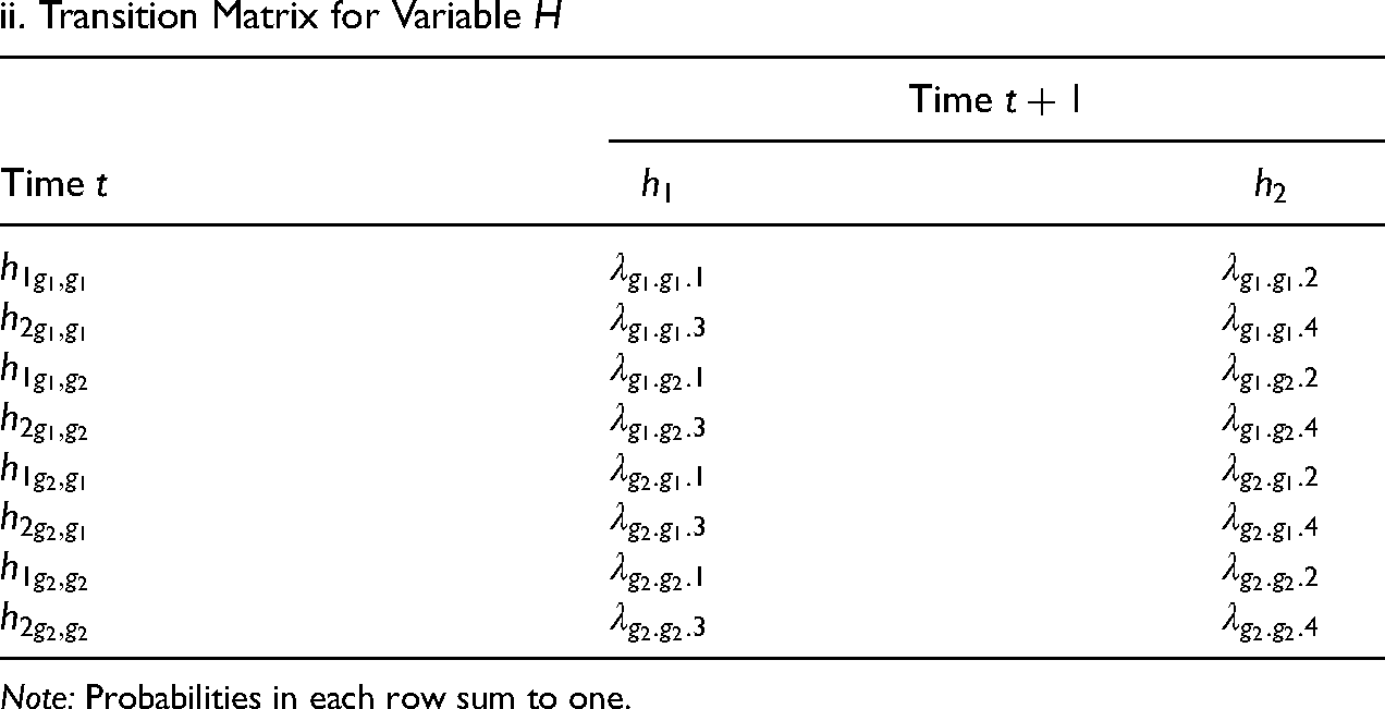
Transition Probabilities of the MMM in Figure 2(b).

i. Transition Matrix for Variable H
	Time $t + 1$
Time t	$h_{1}$	$h_{2}$	$Dead$
$h_{1 g_{1}}$	$σ_{g_{1} .1}$	$σ_{g_{1} .2}$	$σ_{g_{1} .3}$
$h_{2 g_{1}}$	$σ_{g_{1} .4}$	$σ_{g_{1} .5}$	$σ_{g_{1} .6}$
$h_{1 g_{2}}$	$σ_{g_{2} .1}$	$σ_{g_{2} .2}$	$σ_{g_{2} .3}$
$h_{2 g_{2}}$	$σ_{g_{2} .4}$	$σ_{g_{2} .5}$	$σ_{g_{2} .6}$

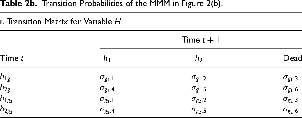
ii. Transition Matrix for Variable G

	Time $t + 1$
Time t	$g_{1}$	$g_{2}$
$g_{1 h_{1}, h_{1}}$	$σ_{h_{1} . h_{1} .1}$	$σ_{h_{1} . h_{1} .2}$
$g_{2 h_{1}, h_{1}}$	$σ_{h_{1} . h_{1} .3}$	$σ_{h_{1} . h_{1} .4}$
$g_{1 h_{1}, h_{2}}$	$σ_{h_{1} . h_{2} .1}$	$σ_{h_{1} . h_{2} .2}$
$g_{2 h_{1}, h_{2}}$	$σ_{h_{1} . h_{2} .3}$	$σ_{h_{1} . h_{2} .4}$
$g_{1 h_{2}, h_{1}}$	$σ_{h_{2} . h_{1} .1}$	$σ_{h_{2} . h_{1} .2}$
$g_{2 h_{2}, h_{1}}$	$σ_{h_{2} . h_{1} .3}$	$σ_{h_{2} . h_{1} .4}$
$g_{1 h_{2}, h_{2}}$	$σ_{h_{2} . h_{2} .1}$	$σ_{h_{2} . h_{2} .2}$
$g_{2 h_{2}, h_{2}}$	$σ_{h_{2} . h_{2} .3}$	$σ_{h_{2} . h_{2} .4}$

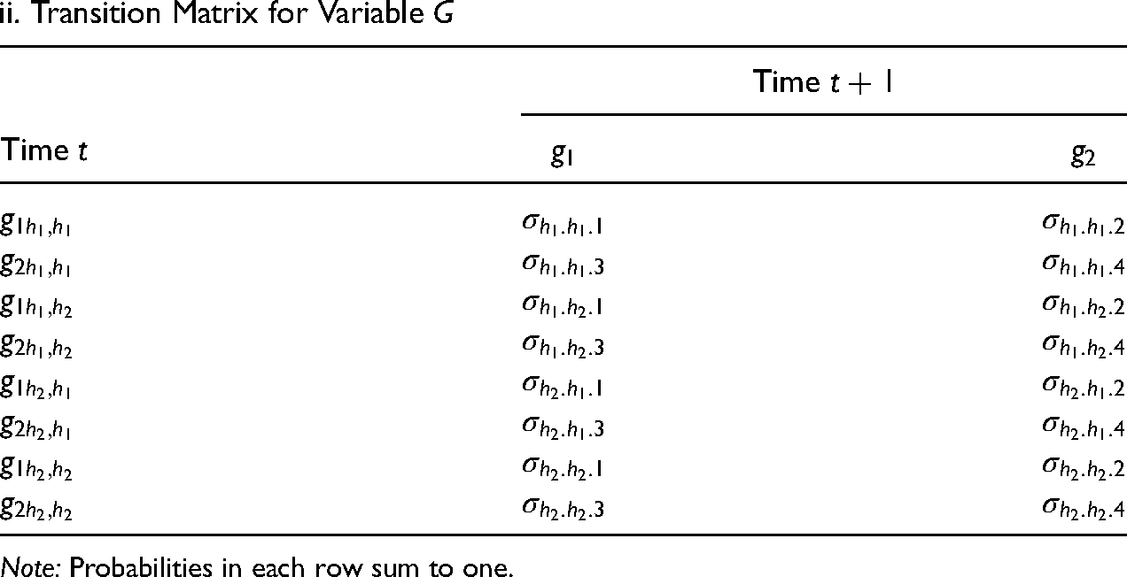
Note: Probabilities in each row sum to one.

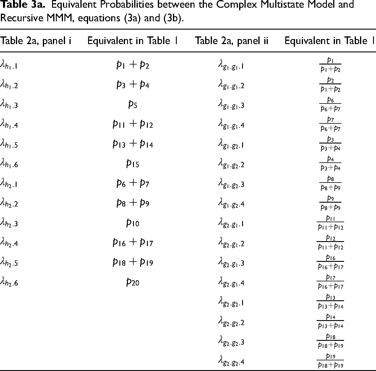
Therefore, transition probabilities in Table 2, panel i have an equivalent relation with those in Table 1. The probability of transitioning to state $g_{1}$ at time $t + 1$ for individuals in states $g_{1}$ and $h_{1}$ (i.e., $λ_{h_{1} .1}$ ), is the joint probability of $Pr (s t a t e_{t + 1} = g_{1} h_{1} | s t a t e_{t} = g_{1} h_{1}, X)$ , or $p_{1}$ , and $Pr (s t a t e_{t + 1} =$ $g_{1} h_{2} | s t a t e_{t} = g_{1} h_{1}, X)$ , or $p_{2}$ . Since $p_{1}$ and $p_{2}$ are mutually exclusive, the joint probability is $p_{1} + p_{2}$ . Similarly, the probability of transitioning to state $g_{2}$ at time $t + 1$ for individuals in states $g_{1}$ and $h_{1}$ (i.e., $λ_{h_{1} .2}$ ), is the joint probability of $p_{3}$ and $p_{4}$ (i.e., $p_{3} + p_{4}$ ). The probability of transitioning to death at time $t + 1$ for individuals in states $g_{1}$ and $h_{1}$ , or $λ_{h_{1} .3}$ is equivalent to $Pr (s t a t e_{t + 1} = Dead | s t a t e_{t} = g_{1} h_{1}, X)$ , or $p_{5}$ . As for panel ii in Table 2a, the probability of a transition in variable H is conditional on a transition in variable G from time t and $t + 1$ . Thus, the probability to transition to state $h_{1}$ given the individual is in states $g_{1}$ and $h_{1}$ at time t and will transition to $g_{1}$ , i.e., $λ_{g_{1} . g_{1} .1}$ , is equivalent to $\frac{p_{1}}{p_{1} + p_{2}}$ , and $λ_{g_{1} . g_{1} .2}$ is equivalent to $\frac{p_{2}}{p_{1} + p_{2}}$ .

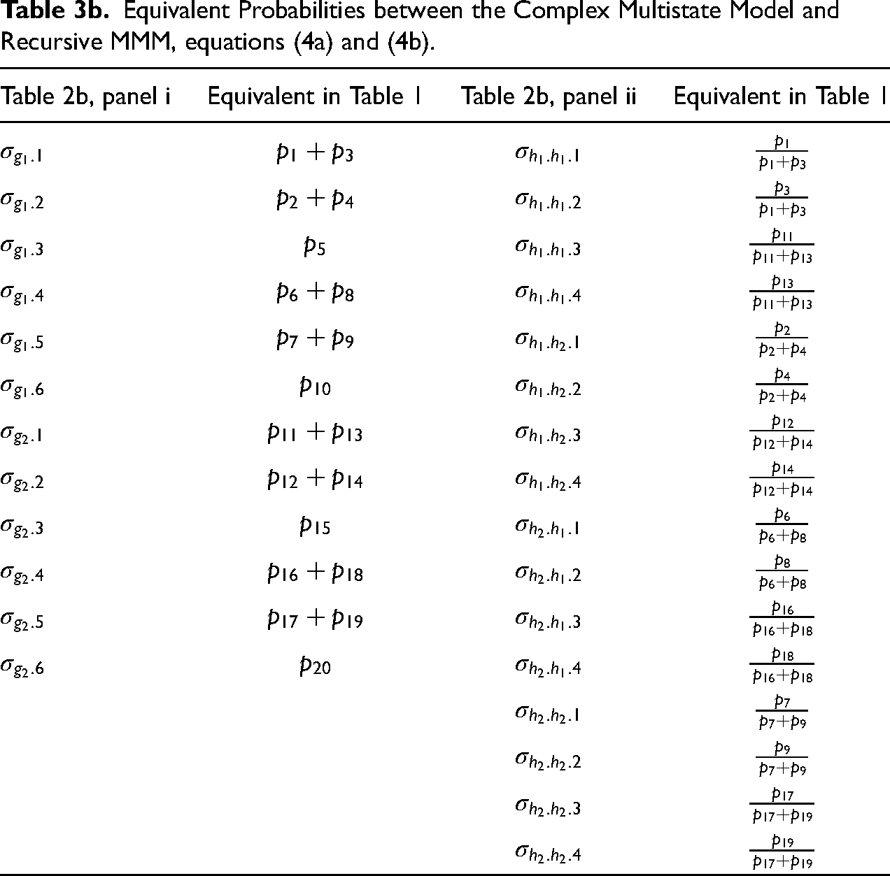
Highly similar equivalencies can be found for Tables 2b and 1. For instance, the transition probability for individuals in states $g_{1}$ and $h_{1}$ transitioning to state $h_{1}$ at time $t + 1$ , i.e., $σ_{g_{1} .1}$ is equivalent to the joint probability of $p_{1}$ and $p_{3}$ (i.e., $p_{1} + p_{3}$ ). We present the equivalence of all probabilities between Tables 1 and 2 in Table 3. Note that we use “equivalent” throughout these paragraphs because all these probabilities are predicted estimates from regressions instead of the observed probabilities and there will be slight variability between models.

Table 3a.

Equivalent Probabilities between the Complex Multistate Model and Recursive MMM, equations (3a) and (3b).

Table 2a, panel i	Equivalent in Table 1	Table 2a, panel ii	Equivalent in Table 1
$λ_{h_{1} .1}$	$p_{1} + p_{2}$	$λ_{g_{1} . g_{1} .1}$	$\frac{p_{1}}{p_{1} + p_{2}}$
$λ_{h_{1} .2}$	$p_{3} + p_{4}$	$λ_{g_{1} . g_{1} .2}$	$\frac{p_{2}}{p_{1} + p_{2}}$
$λ_{h_{1} .3}$	$p_{5}$	$λ_{g_{1} . g_{1} .3}$	$\frac{p_{6}}{p_{6} + p_{7}}$
$λ_{h_{1} .4}$	$p_{11} + p_{12}$	$λ_{g_{1} . g_{1} .4}$	$\frac{p_{7}}{p_{6} + p_{7}}$
$λ_{h_{1} .5}$	$p_{13} + p_{14}$	$λ_{g_{1} . g_{2} .1}$	$\frac{p_{3}}{p_{3} + p_{4}}$
$λ_{h_{1} .6}$	$p_{15}$	$λ_{g_{1} . g_{2} .2}$	$\frac{p_{4}}{p_{3} + p_{4}}$
$λ_{h_{2} .1}$	$p_{6} + p_{7}$	$λ_{g_{1} . g_{2} .3}$	$\frac{p_{8}}{p_{8} + p_{9}}$
$λ_{h_{2} .2}$	$p_{8} + p_{9}$	$λ_{g_{1} . g_{2} .4}$	$\frac{p_{9}}{p_{8} + p_{9}}$
$λ_{h_{2} .3}$	$p_{10}$	$λ_{g_{2} . g_{1} .1}$	$\frac{p_{11}}{p_{11} + p_{12}}$
$λ_{h_{2} .4}$	$p_{16} + p_{17}$	$λ_{g_{2} . g_{1} .2}$	$\frac{p_{12}}{p_{11} + p_{12}}$
$λ_{h_{2} .5}$	$p_{18} + p_{19}$	$λ_{g_{2} . g_{1} .3}$	$\frac{p_{16}}{p_{16} + p_{17}}$
$λ_{h_{2} .6}$	$p_{20}$	$λ_{g_{2} . g_{1} .4}$	$\frac{p_{17}}{p_{16} + p_{17}}$
		$λ_{g_{2} . g_{2} .1}$	$\frac{p_{13}}{p_{13} + p_{14}}$
		$λ_{g_{2} . g_{2} .2}$	$\frac{p_{14}}{p_{13} + p_{14}}$
		$λ_{g_{2} . g_{2} .3}$	$\frac{p_{18}}{p_{18} + p_{19}}$
		$λ_{g_{2} . g_{2} .4}$	$\frac{p_{19}}{p_{18} + p_{19}}$

Table 3b.

Equivalent Probabilities between the Complex Multistate Model and Recursive MMM, equations (4a) and (4b).

Table 2b, panel i	Equivalent in Table 1	Table 2b, panel ii	Equivalent in Table 1
$σ_{g_{1} .1}$	$p_{1} + p_{3}$	$σ_{h_{1} . h_{1} .1}$	$\frac{p_{1}}{p_{1} + p_{3}}$
$σ_{g_{1} .2}$	$p_{2} + p_{4}$	$σ_{h_{1} . h_{1} .2}$	$\frac{p_{3}}{p_{1} + p_{3}}$
$σ_{g_{1} .3}$	$p_{5}$	$σ_{h_{1} . h_{1} .3}$	$\frac{p_{11}}{p_{11} + p_{13}}$
$σ_{g_{1} .4}$	$p_{6} + p_{8}$	$σ_{h_{1} . h_{1} .4}$	$\frac{p_{13}}{p_{11} + p_{13}}$
$σ_{g_{1} .5}$	$p_{7} + p_{9}$	$σ_{h_{1} . h_{2} .1}$	$\frac{p_{2}}{p_{2} + p_{4}}$
$σ_{g_{1} .6}$	$p_{10}$	$σ_{h_{1} . h_{2} .2}$	$\frac{p_{4}}{p_{2} + p_{4}}$
$σ_{g_{2} .1}$	$p_{11} + p_{13}$	$σ_{h_{1} . h_{2} .3}$	$\frac{p_{12}}{p_{12} + p_{14}}$
$σ_{g_{2} .2}$	$p_{12} + p_{14}$	$σ_{h_{1} . h_{2} .4}$	$\frac{p_{14}}{p_{12} + p_{14}}$
$σ_{g_{2} .3}$	$p_{15}$	$σ_{h_{2} . h_{1} .1}$	$\frac{p_{6}}{p_{6} + p_{8}}$
$σ_{g_{2} .4}$	$p_{16} + p_{18}$	$σ_{h_{2} . h_{1} .2}$	$\frac{p_{8}}{p_{6} + p_{8}}$
$σ_{g_{2} .5}$	$p_{17} + p_{19}$	$σ_{h_{2} . h_{1} .3}$	$\frac{p_{16}}{p_{16} + p_{18}}$
$σ_{g_{2} .6}$	$p_{20}$	$σ_{h_{2} . h_{1} .4}$	$\frac{p_{18}}{p_{16} + p_{18}}$
		$σ_{h_{2} . h_{2} .1}$	$\frac{p_{7}}{p_{7} + p_{9}}$
		$σ_{h_{2} . h_{2} .2}$	$\frac{p_{9}}{p_{7} + p_{9}}$
		$σ_{h_{2} . h_{2} .3}$	$\frac{p_{17}}{p_{17} + p_{19}}$
		$σ_{h_{2} . h_{2} .4}$	$\frac{p_{19}}{p_{17} + p_{19}}$

The dashed arrow that connects the two models can also be estimated in two ways as in the CMM: the life table method or through microsimulation. In the life table, the transition probability from time t to $t + 1$ for these two variables can be calculated by multiplying the two relevant probabilities at each age. For example, to obtain the transition probability from states $g_{1}$ and $h_{1}$ at time t to $g_{1}$ and $h_{1}$ at time $t + 1$ at a given age, one could multiply $λ_{h_{1} .1}$ and $λ_{g_{1} . g_{1} .1}$ estimated from equations (3a) and (3b) or $σ_{g_{1} .1}$ and $σ_{h_{1} . h_{1} .1}$ from equations (4a) and (4b). In this case, based on Table 3, both of these quantities are equal to $Pr (s t a t e_{t + 1} = g_{1} h_{1} | s t a t e_{t} = g_{1} h_{1}, X)$ , or $p_{1}$ from equation (1). Therefore, by estimating equations (3a) and (3b) or (4a) and (4b), one can derive the probabilities estimated in equation (2). As such, we demonstrate that both equations (3a) and (3b) and (4a) and (4b) result in the same transition probability after combining the two regression results together, and that they can both replicate the transition probabilities from the CMM.

In this paper, we apply the microsimulation method, but the underlying calculation is the same for the life table method. To get the life/health expectancies, we need the baseline characteristics and transition probabilities. In most cases, the distribution of baseline characteristics can be constructed directly from the longitudinal survey. However, when a large number of baseline characteristics needs to be controlled, the sample size for each group could become very small. In this case, it may be helpful to borrow information from external data sources to construct the baseline. With the baseline, we can proceed to the microsimulation process. As there are more than one set of transition probabilities, we run multiple independent microsimulations for each regression. Taking probabilities from Table 2a as an example, for an individual starting from $g_{1}$ and $h_{1}$ , we first draw a random number from the uniform distribution, $U (0, 1)$ , to determine the next state of variable G according to which subset, in subsets $[0, λ_{h_{1} .1}]$ , $[λ_{h_{1} .1}, λ_{h_{1} .1} + λ_{h_{1} .2}]$ , and $[λ_{h_{1} .1} + λ_{h_{1} .2}, 1]$ , the random number falls into. If the number falls in the first subset, this individual will remain in state $g_{1}$ . Then another random number is drawn from the same uniform distribution to identify the next state of variable H, in subsets $[0, λ_{g_{1} . g_{1} .1}]$ and $[λ_{g_{1} . g_{1} .1}, 1]$ . This process continues over age, obtaining the subsequent states of variables G and H for this individual year by year. Alternatively, if the number falls in the third subset, then the second random number is not needed since this individual remains dead in all the future states.

So far, we have shown that the recursive MMM can exactly replicate the CMM. By disentangling one regression into multiple regressions, our approach facilitates more flexibility in model design. Modeling each coevolving variable with its own regression means that it is possible to modify or optimize the regressions for these variables separately. To be more specific, borrowing the idea from the reduced-form VAR concept, the MMM could incorporate time-varying variables with complex models by allowing researchers to reduce insignificant interactions and manipulate the relationship between coevolving variables according to their research questions and theoretical framework. We further demonstrate the flexibility of modeling with the MMM framework by walking through real-life examples of different MMM models in the Applications section.

Applications

In this section, we first compare results from two MMM models with recursive and reduced-form VAR against the results from a five-state multistate model focusing on two dimensions of health as in Shen and Payne (2023). By this comparison, we demonstrate how the reduced-form VAR model can be used to estimate multistate life table quantities in complex state spaces, reducing estimation difficulties through removing less important interactions. For a second example, we further present how the MMM can be applied to incorporate other time-varying variables. This example uses the MMM to explore healthy life expectancy while accounting for changes in marital status.

Data

Data for both application examples are from the U.S. HRS (Health and Retirement Study 2021), a bi-annual national longitudinal survey (Sonnega et al. 2014). In example 1, our analyses use data from 1998 to 2018 of the HRS to estimate cohort partial health expectancy with disability and morbidity across birth cohorts. Disability and morbidity are defined the same way as in Shen and Payne (2023). Disability is classified into two categories: “Disability-free” (DF) and “Activities of Daily Living (ADL) disabled” (D). Individuals are classified as “Morbid” (M) if they have ever been diagnosed with any of the five chronic diseases including cancer, diabetes, heart disease, lung disease, and stroke, and “Morbidity-free” (MF) otherwise.

In the second example, we use data from the 2008 to 2018 waves of the HRS to estimate remaining healthy life expectancy by sex and marital status for those aged 55 plus. Marital status is divided into three categories: “married/partnered,” “divorced/separated,” and “widowed/widower.” Individuals who never married are excluded from the analyses as they are a very small population and are unlikely to change marital status over time in older cohorts. Health is defined by self-rated health, where individuals who responded “Excellent” or “Very good” are reclassified as “very good,” “Good” as “fair,” and “Fair” or “Poor” as “poor.”

Example 1: Two Dimensions of Health

Figure 3 describes the CMM and state space in Shen and Payne (2023), replacing the variables G and H in the Method section to Morbidity and Disability. Note that the state space is slightly constrained as compared to Figure 1, as transitions from morbid to morbidity-free are not allowed under the definition of morbidity as ever diagnosed. In this CMM, the transition probabilities are estimated using a single multinomial logistic regression as shown below:

logit (s t a t e_{t + 1}) = β_{0} + β_{1} \cdot s t a t e_{t} + β_{2} \cdot a g e_{t} + β_{i} \cdot X_{i},

(5)

where

X_{i}

includes terms for age-squared, sex, birth cohorts, and interactions between age, sex, and birth cohorts.

Figure 3.

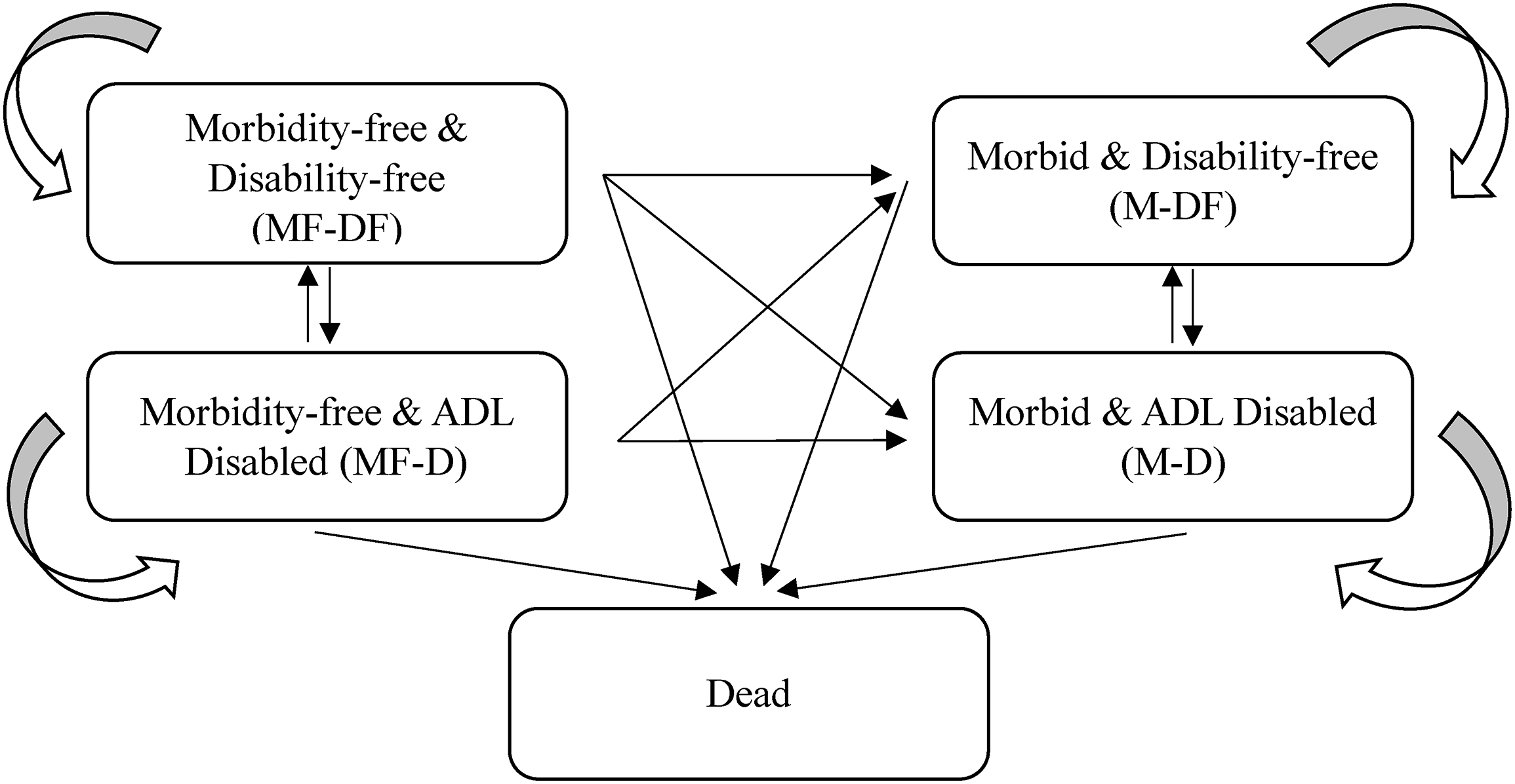
Complex multistate model with disability and morbidity.

Here, we estimate this same five-state model with the MMM framework. First, we demonstrate the MMM with recursive VAR(1), which has highly similar procedures as what is described in the Method section. Variable G is replaced by morbidity and variable H by disability as follows:

\begin{aligned} logit (m o r b i d i t y_{t + 1}) = & β_{m 0} + β_{m 1} m o r b i d i t y_{t} + β_{m 2} d i s a b i l i t y_{t} \\ + β_{m 3} a g e_{t} + β_{m i} X_{i}, \end{aligned}

(6\rm a)

logit (d i s a b i l i t y_{t + 1}) = β_{d 0} + β_{d 1} d i s a b i l i t y_{t} + β_{d 2} m o r b i d i t y_{t} + β_{d 3} m o r b i d i t y_{t + 1} + β_{d 4} a g e_{t} + β_{d} X_{i},

(6\rm b)

where

X_{i}

includes terms for age-squared, sex, birth cohorts, and interactions between age, sex, and birth cohorts, interactions between age, morbidity, and disability as well as interactions between sex, morbidity, and disability. The state space and the transition probability can be obtained from Figure 2(a) and Table 2a, respectively by substituting variable G to Morbidity and variable H to Disability, where

g_{1}

and

g_{2}

correspond to “MF” and “M” respectively, and

h_{1}

and

h_{2}

to “DF” and “D.”

In this section, we focus on describing and comparing one of the potential alternatives that utilizes features of the reduced-form MMM to reduce complexity in the state space. This MMM would be estimated by

\begin{aligned} logit (d i s a b i l i t y_{t + 1}) & = β_{d 0} + β_{d 1} m o r b i d i t y_{t} + β_{d 2} d i s a b i l i t y_{t} \\ + β_{d 3} a g e_{t} + β_{d i} X_{i}, \end{aligned}

(7\rm a)

logit (m o r b i d i t y_{t + 1}) = β_{m 0} + β_{m 1} m o r b i d i t y_{t} + β_{m 2} d i s a b i l i t y_{t} + β_{m 3} a g e_{t} + β_{m i} X_{i},

(7\rm b)

where

X_{i}

similarly includes terms for age-squared, sex, birth cohorts, and interactions between age, sex, and birth cohorts, interactions between age, morbidity, and disability, as well as interactions between sex, morbidity, and disability. To retain the non-linear relationship, interaction terms between age, morbidity, and disability at time t are also included. As discussed in the Method section, only one of the regressions needs to estimate the transition to mortality, and the choice of which regression includes mortality does not matter in the simulation results. Here, we model the transition probability to death alongside disability status. In other words,

d i s a b i l i t y_{t + 1}

has three states (i.e., DF, D, and dead) and

m o r b i d i t y_{t + 1}

has two states (i.e., MF and M). Figure 4 and Table 4 illustrate the state space and the corresponding probabilities of this specific model.

Figure 4.

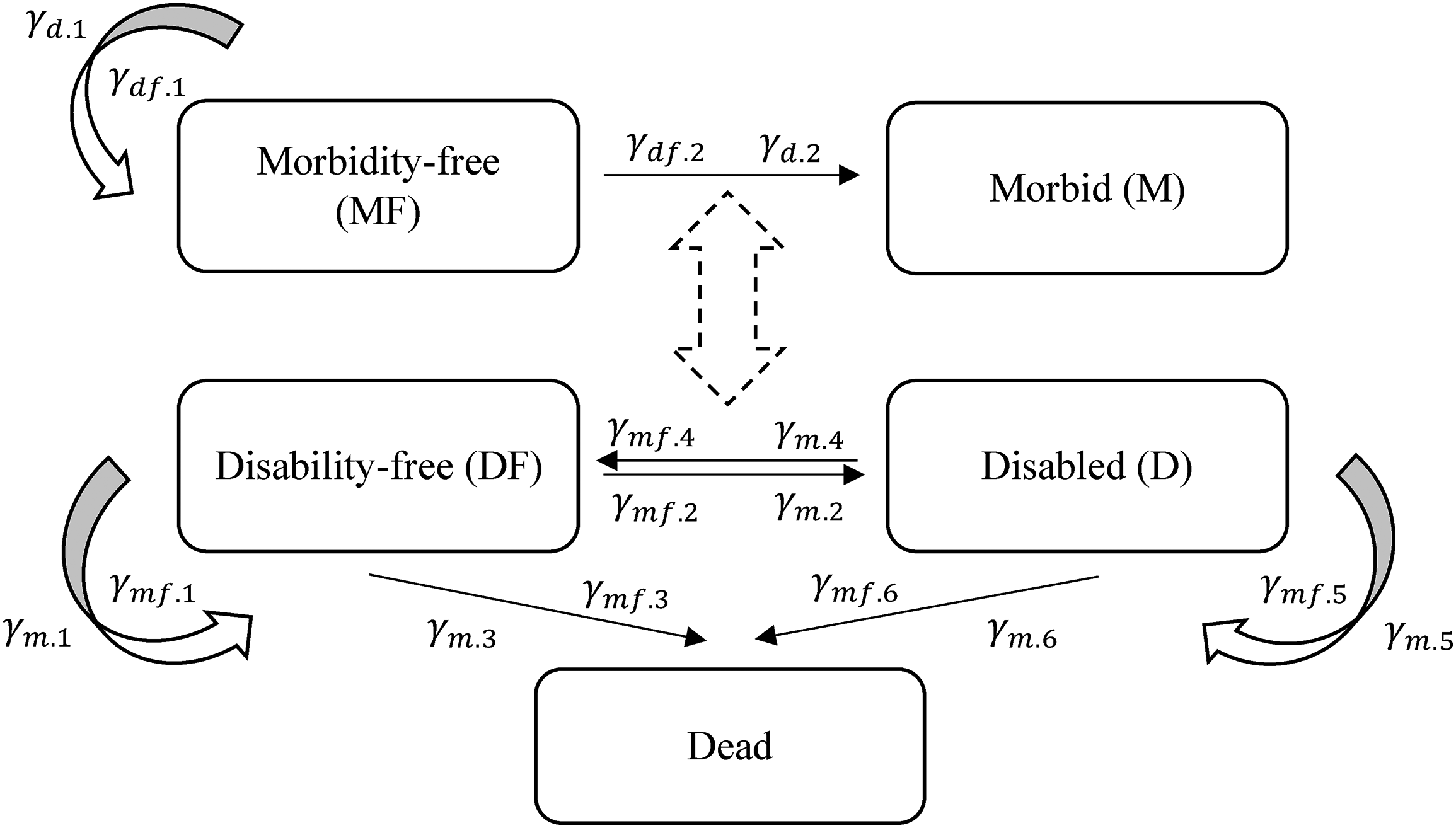
Multiple multistate method with reduced-form VAR(1).

Table 4.

Transition Probabilities of the MMM in Figure 4.

i. Transition Matrix for Morbidity
Time t	Time $t + 1$
Time t	MF	M
${MF}_{d f}$	$γ_{d f .1}$	$γ_{d f .2}$
$M_{d f}$	0	1
${MF}_{d}$	$γ_{d .1}$	$γ_{d .2}$
$M_{d}$	0	1

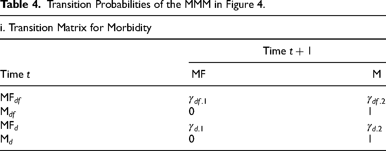
ii. Transition Matrix for Disability

Time t	Time $t + 1$
Time t	$DF$	$D$	$Dead$
${DF}_{m f}$	$γ_{m f .1}$	$γ_{m f .2}$	$γ_{m f .3}$
$D_{m f}$	$γ_{m f .4}$	$γ_{m f .5}$	$γ_{m f .6}$
${DF}_{m}$	$γ_{m .1}$	$γ_{m .2}$	$γ_{m .3}$
$D_{m}$	$γ_{m .4}$	$γ_{m .5}$	$γ_{m .6}$

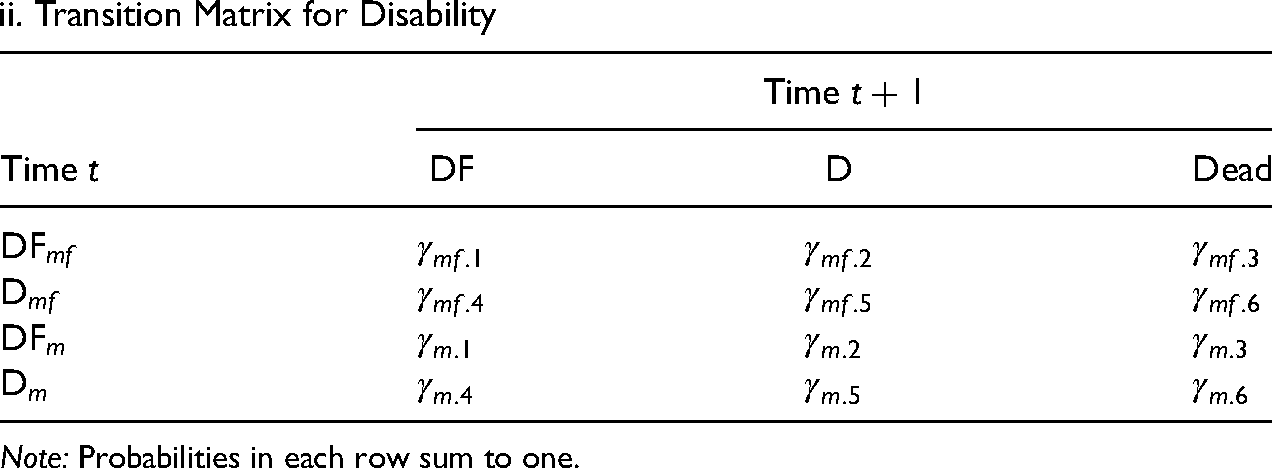
Note: Probabilities in each row sum to one.

Figure 4 is similar to the recursive MMM in Figure 2(a). In panel i of Table 4, the transition matrix for morbidity is almost the same as panel i in Table 2a. Transitions between morbidity states rely on morbidity and disability at time t. The major difference is in panel ii of Table 4 (the transition matrix for disability), where disability at time $t + 1$ is only dependent on morbidity and disability at time t (e.g., $\Pr (d i s a b i l i t y_{t + 1} = DF | m o r b i d i t y_{t} = MF, d i s a b i l i t y_{t} = DF, X)$ is $γ_{m f \cdot 1}$ ), instead of being dependent on disability at time t and morbidity at time t and $t + 1$ .

Since the reduced-form VAR estimated fewer parameters in exchange for a more parsimonious model, unlike the recursive MMM, the reduced-form MMM cannot derive the exact probabilities in the CMM. More specifically, the relationship between contemporaneous changes in the two dimensions of health (or time-varying variables) is not controlled. For example, an individual with $m o r b i d i t y_{t} = MF$ and $d i s a b i l i t y_{t} = DF$ will have the same probability of transitioning to $d i s a b i l i t y_{t + 1} = DF o r D$ regardless of their morbidity state at time $t + 1$ . Conceptually speaking, this is not a bad approximation. People are most likely to be diagnosed with morbidities at the early stage of the disease with mild symptoms (i.e., no disability). The impact of a given disease accumulates over the life course and may lead to higher chances of being disabled at older ages. Most of the effects of chronic diseases are accumulative rather than the result of an instant shock to the body (Chou et al. 2021), hence morbidity and disability onsets are unlikely to be contemporaneous. However, this assumption may not hold true with other variables. For example, if the other event is not morbidity but instead a measure of whether the individual had experienced a fall, there would likely be a very strong concurrent relationship between falls and disability. Additionally, the accumulative effect would be very small. In other words, a person who experienced a fall and was not disabled in the first year may indicate that they were not severely injured and are not more likely to be disabled in the future years due to the fall. Therefore, like all other modeling, it is important to justify the selection of model with the empirical and theoretical evidence.

A comparison of results from the complex multistate method and two types of MMM (recursive and reduced-form) is presented in Table 5 and in Figures A1–A3. Table 5 presents health expectancies calculated through three models: complex five-state model (CMM), MMM with recursive VAR(1), and MMM with reduced-form VAR(1); inside the parentheses are 95 percent confidence intervals from bootstrapping. For brevity, we only show the results at age 70 from cohort 1934–1943 (the full comparison for all age groups can be found in Figures A1 and A2 in the Appendix). The three models have very close point estimates for all expectancies, with differences under 0.1 for all expectancies. Based on the confidence intervals, none of them are significantly different from one another. Note that the source of uncertainty in the MMM is somewhat different from that in the CMM, as in MMM the uncertainties are combined from separate equations through microsimulation. Nonetheless, the bootstrapping technique (Kulesa et al. 2015) still captures the individual variation in the data and the confidence intervals are very similar. In Figures A1 and A2, the MMM model is compared to the CMM. The figures are superimposed on each other so that it is easier to examine the difference. Figure A3 further disaggregates results in Figure A2 by initial morbidity status, which is a type of status-base life expectancy. Similar to Table 5, none of the age and gender groups are significantly different.

Table 5.

Partial Health Expectancies of Various Health States (Age 70–79 for Cohort 1934–1943): Comparison of Three Models.

Gender	Health state	Traditional five-state	MMM (recursive)	MMM (reduced-form)
Men	MF-DF	2.56 (2.38, 2.75)	2.54 (2.38, 2.71)	2.52 (2.34, 2.67)
	MF-D	0.25 (0.20, 0.31)	0.25 (0.21, 0.28)	0.28 (0.24, 0.32)
	M-DF	4.84 (4.65, 5.02)	4.82 (4.67, 5.01)	4.89 (4.73, 5.07)
	M-D	0.99 (0.92, 1.09)	1.01 (0.93, 1.08)	0.97 (0.89, 1.05)
	Total	8.64 (8.57, 8.73)	8.62 (8.55, 8.72)	8.66 (8.57, 8.73)
Women	MF-DF	3.31 (3.13, 3.46)	3.27 (3.11, 3.43)	3.24 (3.07, 3.39)
	MF-D	0.34 (0.30, 0.40)	0.36 (0.31, 0.39)	0.38 (0.34, 0.43)
	M-DF	4.04 (3.87, 4.20)	4.05 (3.91, 4.22)	4.10 (3.97, 4.27)
	M-D	1.31 (1.21, 1.41)	1.33 (1.24, 1.42)	1.28 (1.19, 1.37)
	Total	8.99 (8.93, 9.08)	9.01 (8.93, 9.07)	9.00 (8.94, 9.08)

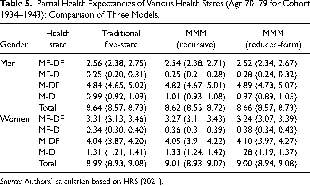
Source: Authors’ calculation based on HRS (2021).

To produce these similar results, the reduced-form MMM is simpler, with fewer interaction terms. The benefit of reduced-form MMM is apparent by looking at the number of transitions between health states in Table 6. We show the transitions modeled in CMM in panel a, and in reduced-form MMM in panel b. The dependent variables (i.e., health status at time $t + 1$ ) have fewer categories because they are now estimating the joint probability. Fewer categories mean larger sample sizes in each category and more reliable estimates, especially if a given transition is rare in some groups. For example, the smallest sample is between MF-D to M-DF with 45 observed events across age in panel a, while in panel b the smallest number of observed events is 132 other than transitions to death. Although 45 events are not a small sample, this is only a five states example that could be handled easily by the CMM (e.g., Bardenheier et al. 2016; Laditka et al. 2021). In example 2, we apply the MMM to a more complex model to better demonstrate the advantages of the MMM.

Table 6.

Transitions between Various Health States in Example 1 (Cohort 1934–1943 Age 70–79).

a. CMM, equation (5)
Time t	Time $t + 1$
Time t	MF-DF	MF-D	M-DF	M-D	Death
MF-DF	14,288	397	890	115	149
MF-D	276	1,152	45	87	45
M-DF	–	–	20,561	1,174	590
M-D	–	–	686	4,789	537

b. Reduced-form MMM, equations (7a) and (7b)

i. Disability (equation (7a))				ii. Morbidity (equation (7b))
Time t	Time $t + 1$			Time t	Time $t + 1$
Time t	DF	D	Death	Time t	MF	M	Death^a
MF-DF	15,178	512	149	MF-DF	14,685	1,005	149
MF-D	321	1,239	45	MF-D	1,428	132	45
M-DF	20,561	1,174	590	M-DF	–	21,735	590
M-D	686	4,789	537	M-D	–	5,475	537

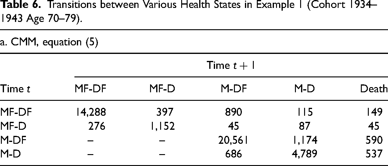
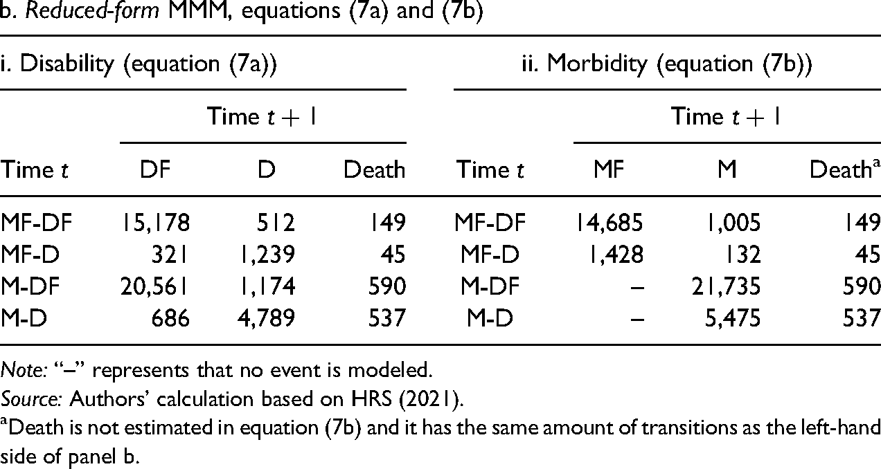
Note: “–” represents that no event is modeled.

Source: Authors’ calculation based on HRS (2021).

Death is not estimated in equation (7b) and it has the same amount of transitions as the left-hand side of panel b.

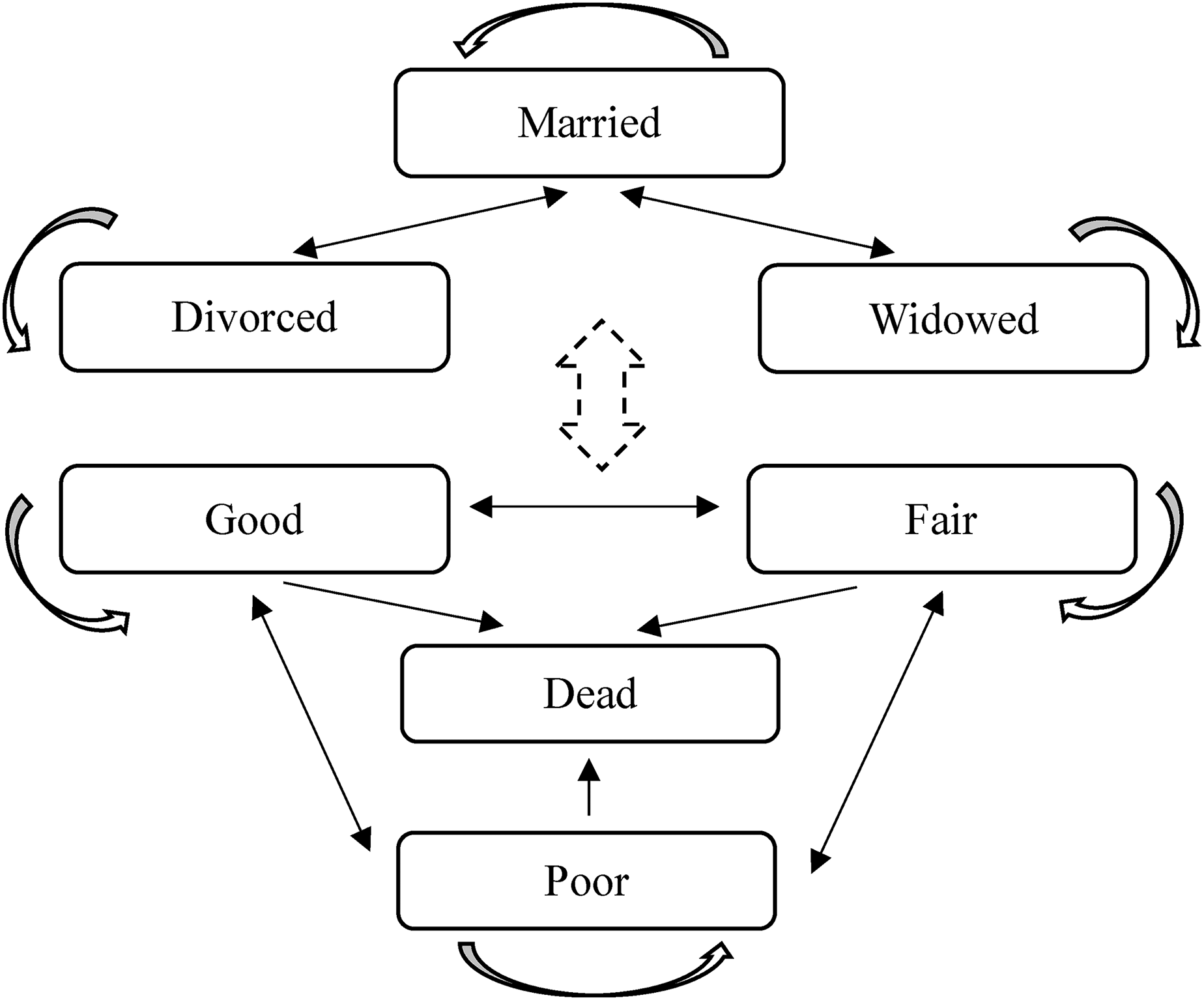
Example 2: Marital Status and Healthy Life Expectancy

As a second example to demonstrate the flexibility of the MMM, we apply the MMM to model self-rated health and marital status. Each outcome has three categories, leading to a state space of 10 states which is quite large to estimate using the CMM. Furthermore, marital status and health could coevolve over time but are very different domains of the life course. Even though there are papers (Goldman et al. 1995; Jia and Lubetkin 2020; Rendall et al. 2011) about the association between marital status and health/survival, the mechanism is likely to be indirect through behavior change (Wilson and Oswald 2005), social support (Becker et al. 2019; Berkman 1984), and other long-term accumulated processes (Verbrugge 1979). Thus, it is a good case to demonstrate the advantages of the MMM when the contemporaneous relationship between outcomes is theorized to be weak.

Marriage selection theory suggests that healthier individuals are more likely to get married (Goldman 1993; Murray 2000). In our analyses below, we exclude the never-married group. We also hypothesize that, conditional on being ever married, the current health of the respondent is likely not a strong predictor of marital status but not the other way around. We deploy this hypothesis partly because it is conceptually plausible and partly because we want to demonstrate the flexibility of the MMM. Therefore, this hypothesis can be removed depending on the research question. The regression models are constructed as follows:

logit (h e a l t h_{t + 1}) = β_{h 0} + β_{h 1} m a r i t a l_{t} + β_{h 2} h e a l t h_{t} + β_{h 3} a g e_{t} + β_{h 4} s e x

(8\rm a)

logit (m a r i t a l_{t + 1}) = β_{m 0} + β_{m 1} m a r i t a l_{t} + β_{m 2} a g e_{t} + β_{m 3} s e x

(8\rm b)

The transitions and state space of the model are illustrated in Figure 5. We also limit the state space to not allow direct transitions between divorced and widowed. The transition to death could be estimated in either regression, but it is modeled with self-rated health in our calculation. Table 7 shows the number of transitions between self-rated health and marital status in a traditional CMM setup and the MMM model. If the transition matrix is modeled in a single multinomial logit as in the CMM, the regression is likely run into convergence issues as there are eight cells with 20 or fewer events in panel a. In contrast, the smallest number of transition events is 70 in panel b. Therefore, the number of transitions being modeled is much larger using the MMM.

Figure 5.

Marital status and health with MMM.

Table 7.

Transitions between Self-Rated Health and Marital Status Example 2.

a. CMM
Time t	Time $t + 1$
Time t	MG	MF	MP	DG	DF	DP	WG	WF	WP	Death
MG	35,103	4,287	989	167	62	19	470	190	62	360
MF	3,661	25,136	3,066	71	106	67	152	350	160	586
MP	693	2,543	20,614	26	54	227	41	162	438	1,465
DG	137	50	20	5,861	771	225	-	-	-	70
DF	44	92	29	666	5,427	757	-	-	-	117
DP	14	36	137	167	736	6,799	-	-	-	423
WG	76	25	8	-	-	-	7,874	1109	420	365
WF	11	40	10	-	-	-	950	7723	1,223	549
WP	4	15	47	-	-	-	276	918	9,442	1,363

b. MMM, equations (8a) and (8b)
i. Self-rated health (equation (8a))					ii. Marital status (equation (8b))
	Time $t + 1$				Time t	Time $t + 1$
Time t	G	F	P	Death	Time t	M	D	W	Death^a
MG	35,740	4,539	1,070	360	M	96,092	799	2,025	2,411
MF	3,884	25,592	3,293	586
MP	760	2,759	21,279	1,465
DG	5,998	821	245	70	D	559	21,409	-	610
DF	710	5,519	786	117
DP	181	772	6,936	423
WG	7,950	1,134	428	365	W	236	–	29,935	2,277
WF	961	7,763	1,233	549
WP	280	933	9,489	1,363

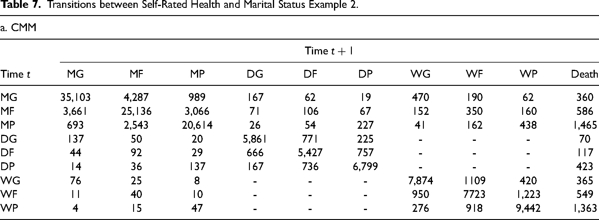
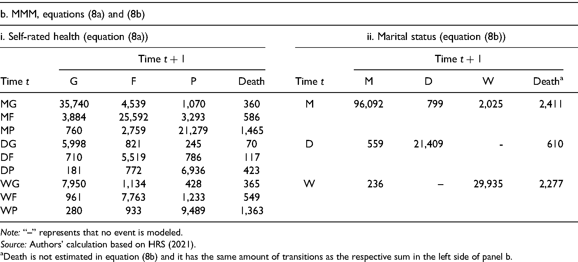
Note: “–” represents that no event is modeled.

Source: Authors’ calculation based on HRS (2021).

Death is not estimated in equation (8b) and it has the same amount of transitions as the respective sum in the left side of panel b.

Since marital status varies over time, the population-averaged expectancies at any age are rather difficult to interpret and understand. Instead, we group individuals based on the period in the life-course that a marital status change occurs to explore the potential health impacts of a marital dissolution (i.e., becoming divorced or widowed) on remaining healthy life expectancy, and how these may change over age. Table 8 presents the results of the remaining healthy life expectancy by gender and age according to the timing of a change in marital status. The first group of people remains married from age 55 to the starting age of remaining life expectancy and the other group experience at least once marital dissolution within a certain age range (also including people who change back to married within that age range). For example, a married man at age 55 who remained married at 64 could expect 7.40 years healthy life expectancy and a total of 19.09 years of total remaining life expectancy remaining at age 65. In contrast, a married man at age 55 who experienced a marital dissolution between 55 and 64 could expect to live only 6.08 years of healthy life and 17.63 years of total remaining life at age 65.

Table 8.

Remaining Healthy Life Expectancy by Marital Status and Age.

Gender	Starting age (age range)	Health state	Remain married	Changed to non-married
Men	65 (55–64)	Good	7.40 (7.04, 7.73)	6.08 (5.69, 6.54)
		Fair	6.63 (6.38, 6.88)	6.17 (5.86, 6.52)
		Poor	5.07 (4.81, 5.33)	5.35 (5.02, 5.71)
		Total	19.09 (18.75, 19.47)	17.63 (17.07, 18.23)
	75 (65–74)	Good	4.31 (4.05, 4.58)	3.53 (3.25, 3.82)
		Fair	4.20 (4.00, 4.42)	3.83 (3.59, 4.09)
		Poor	3.60 (3.40, 3.81)	3.75 (3.48, 4.03)
		Total	12.12 (11.81, 12.44)	11.11 (10.72, 11.54)
	85 (75–84)	Good	2.22 (2.00, 2.43)	1.88 (1.68, 2.11)
		Fair	2.30 (2.14, 2.49)	2.15 (1.95, 2.34)
		Poor	2.24 (2.05, 2.45)	2.40 (2.18, 2.62)
		Total	6.76 (6.46, 7.07)	6.41 (6.16, 6.75)
Women	65 (55–64)	Good	8.88 (8.58, 9.23)	7.49 (7.12, 7.87)
		Fair	7.25 (7.00, 7.52)	6.87 (6.54, 7.17)
		Poor	5.84 (5.58, 6.09)	6.27 (5.97, 6.58)
		Total	21.98 (21.61, 22.35)	20.64 (20.16, 21.10)
	75 (65–74)	Good	5.26 (5.00, 5.54)	4.47 (4.23, 4.75)
		Fair	4.87 (4.66, 5.09)	4.54 (4.33, 4.77)
		Poor	4.26 (4.06, 4.47)	4.54 (4.29, 4.75)
		Total	14.39 (14.09, 14.72)	13.55 (13.21, 13.86)
	85 (75–84)	Good	2.72 (2.47, 2.99)	2.39 (2.20, 2.59)
		Fair	2.84 (2.65, 3.04)	2.70 (2.52, 2.86)
		Poor	2.74 (2.55, 2.95)	2.96 (2.78, 3.17)
		Total	8.30 (8.02, 8.60)	8.05 (7.77, 8.31)

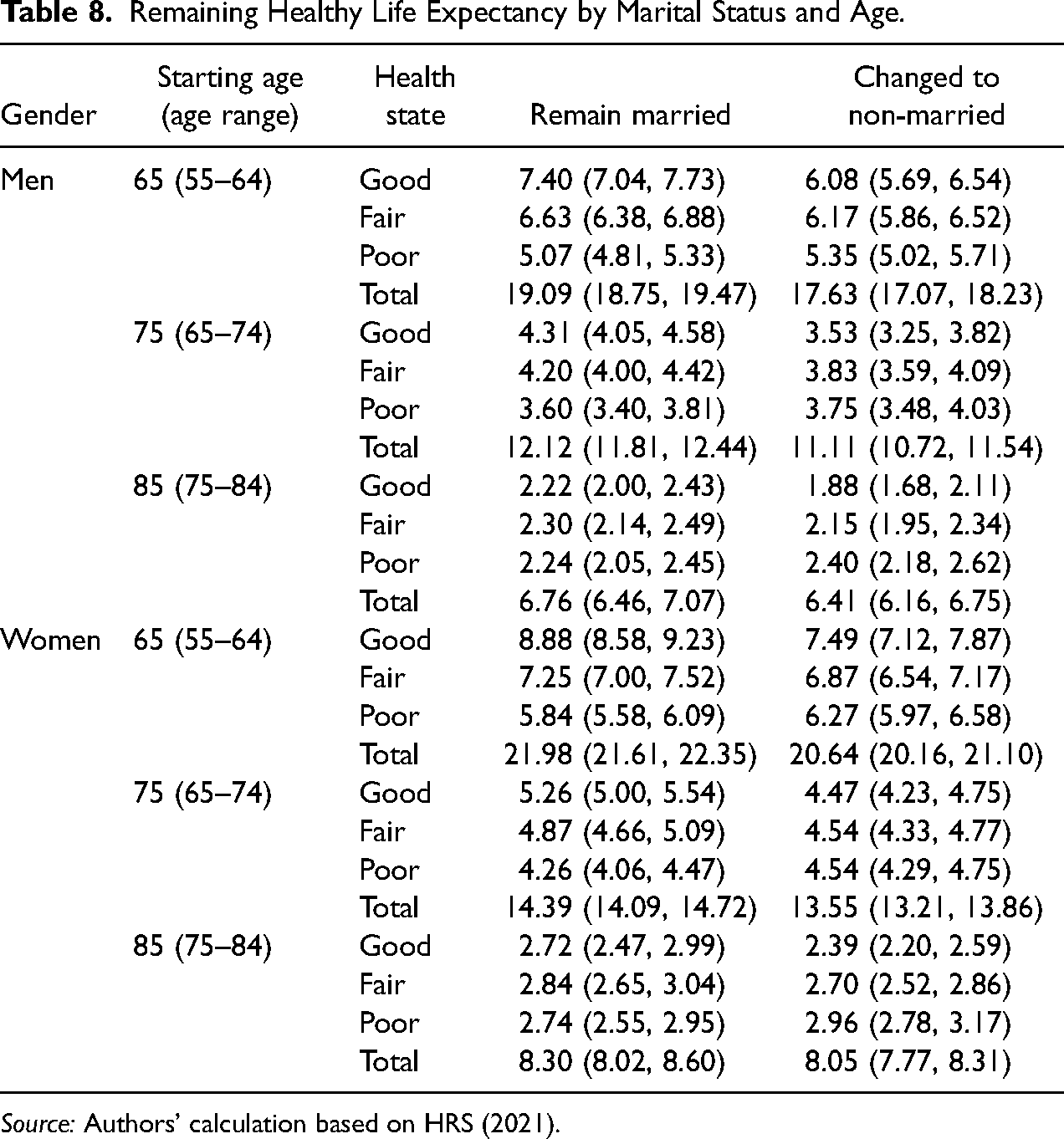
Source: Authors’ calculation based on HRS (2021).

In general, individuals who stay married over the period have higher remaining life expectancy. The two groups are also significantly different in their remaining healthy life expectancy at ages 65 and 75, and in the percentage of remaining life lived in good health. However, this beneficial effect on health and survival diminishes with increasing age. Though insignificant, individuals who remain married at age 85 have a slightly higher healthy life expectancy compared to those who experience a marital dissolution between 75 and 84. As expected, women's healthy life expectancy and total life expectancy are always higher than men's at the same age. This is only one of the research questions we can answer by these simulated individual trajectories. It is possible to explore a number of more specific questions, e.g., the number of transitions between self-rated health states in the 5 years after a married woman becomes a widow.

Discussion and Conclusion

This paper introduces and develops a flexible method, MMM, to estimate health expectancy in models with more than one coevolving variable. Previously, time-varying variables other than the main health indicator would either be assumed static in the health expectancy estimation or be incorporated into the state space. Neither of these methods has been widely used, as they both come with substantial drawbacks: the static assumption may not be realistic in many cases, and the sample size required to estimate the complex state space is larger than available in most longitudinal data sources. In addition, the multistate model is used in modeling transitions and durational expectancies in research on labor force status (Hayward and Lichter 1998; Studer, Struffolino and Fasang 2018), marital status (Schoen and Canudas-Romo 2006; Willekens et al. 1982; Zeng et al. 2012), and migration (Land and Rogers 1982; Raymer, Willekens and Rogers 2019). Thus, the method is not confined to health expectancy, and it could be used to explore other durational expectancies based on the multistate model. Our approach opens new research directions using detailed state spaces that are unfeasible to explore using the standard CMM.

The MMM can fully reproduce the CMM, but the advantage of the MMM lies in its flexibility to trade off reductions in interaction terms for greater complexity in the modeled state space. As shown in the first example, the MMM with reduced interactions produces very similar results as compared to the CMM. Furthermore, the second example also presents coherent findings with other related studies. Our results provide similar evidence on the protective effect of marriage on survival and health that is suggested in Rendall et al. (2011) and Jia and Lubetkin (2020). The protection effect also fades over age as found in other studies. Robards et al. (2012) suggest that when it comes to the elderly, other time-varying variables may also be important, such as living arrangements, which are highly correlated with marital status.

With the MMM, it is feasible to generalize our framework and apply it to estimate more than two time-varying variables at a time. Although our example only presents two coevolving variables, the advantage of the MMM is that it makes estimation of even larger state spaces possible, and can estimate models with multiple coevolving variables and large numbers of outcome categories. Furthermore, the MMM approach could also be combined with Bayesian multistate life table methods (Lynch and Zang 2022) to address very complicated research questions with many coevolving variables and a relatively large state space in each of these variables.

As is common in statistical modeling, the reduced complexity of the MMM approach does come with a stronger set of assumptions than the CMM. By providing a toolkit to flexibly reduce interaction terms, the MMM approach substantially expands the complexity of multistate models that can be estimated using longitudinal sample survey data. Reducing these interaction terms can most clearly have an impact in cases where the two time-varying variables of interest have a strong contemporaneous relationship—that is, where a change in one variable has a strong, immediate impact on the likelihood of a change in the other variable(s). However, what interactions to include, and what to drop, is a question that must be largely guided by theory and previous evidence.

There are other limitations (or assumptions) related to a multistate method. The multistate life table is essentially a discrete-time Markov process. One of the Markov properties is that it is a memoryless system, where the immediate next state only depends on the current state. This is a common limitation of studies using multistate life table with left-censored survey data. Cai, Schenker, and Lubitz (2006) combined the semi-Markov model with a backward simulation algorithm to impute the starting point and avoid the left-censored issue. This is a promising method to relax the Markov assumption by incorporating the duration dependence but has not been widely used due to the small sample size and the short follow-up period of most social surveys. Another limitation lies in the discrete-time approach and the assumption of no unobserved transitions between time points. The main reason for this approach is that HRS (and many other health surveys) are conducted about every 2 years. Our paper presents the MMM using an event-history approach in line with Crimmins, Hayward and Saito (1994) and Cai et al. (2010). A possible extension to the MMM is to adopt the embedded Markov model (EMC) approach by Laditka and Wolf (1998). Wolf and Gill (2009) suggest that compared to the event-history model, EMC may perform better in certain contexts, although it is not fully unbiased. EMC assumes multiple unobserved transitions between observed intervals. It is possible to apply a similar estimation procedure as the EMC model to estimate the multiple multinomial logistic regressions in the MMM framework. With the foundation laid in this paper, further research could explore this possibility and potential caveats. A recent study by Dudel and Schneider (2023) also presents a way to quantify the potential bias from this assumption. Thus, it is important to bear these biases in mind when using the MMM and interpreting the results.

In conclusion, MMM provides researchers with a powerful tool to estimate health expectancy with more than one time-varying variable and in complex state spaces. Although expectancy-based models are most common in estimating health expectancies, our approach could be used to explore a number of other durational expectancies such as time in employment, homelessness, and marriage. Overall, MMM represents a flexible approach to estimating durational expectancies in complex models based on longitudinal sample survey data, and one that makes a wider array of social research questions possible in the multistate framework.

Supplemental Material

sj-pdf-1-smr-10.1177_00491241241268775 - Supplemental material for Dynamics of Health Expectancy: An Introduction to the Multiple Multistate Method (MMM)

Supplemental material, sj-pdf-1-smr-10.1177_00491241241268775 for Dynamics of Health Expectancy: An Introduction to the Multiple Multistate Method (MMM) by Tianyu Shen, Collin F. Payne and Maria Jahromi in Sociological Methods & Research

Footnotes

Declaration of Conflicting Interests

The authors declared no potential conflicts of interest with respect to the research, authorship, and/or publication of this article.

Funding

The authors disclosed receipt of the following financial support for the research, authorship, and/or publication of this article: This work was supported by the Australian Research Council (grant number DE210100087) and also by an ANU Futures Scheme Award funded by the Australian National University.

ORCID iDs

Tianyu Shen

Collin F. Payne

Maria Jahromi

Data Availability Statement

The data used in this study are available in HRS website, https://hrsdata.isr.umich.edu/data-products/rand-hrs-longitudinal-file-2018. Our analysis is conducted in R software (R Core Team 2023). The R scripts to produce the results are available at .

Supplemental Material

Supplemental material for this article is available online.

Author Biographies

Tianyu Shen is a PhD candidate in the School of Demography at the Australian National University. His PhD thesis centers on the analysis of social inequalities in health and the advancement of multistate models to capture population dynamics. His articles have appeared in leading demographic journals, such as Demography, Population Studies and Population Space and Place.

Collin F. Payne is an associate professor in the School of Demography at the Australian National University and a visiting faculty member at the Harvard Center for Population and Development Studies. He is an ARC DECRA Fellow and an associate investigator at the ARC Centre of Excellence in Population Ageing Research. He holds a PhD in demography from the University of Pennsylvania. His work focuses on understanding the dynamics of chronic health conditions, disability, frailty, and multimorbidity over time and across generations using multistate models and demographic microsimulation. His research has appeared in leading demographic and health journals including Demography, Population and Development Review, PLoS Medicine, and The Lancet HIV.

Maria Jahromi is a senior lecturer (assistant professor) in applied economics at POLIS: The Centre for Social Policy Research at the Australian National University. She is a Centre Affiliate at the ANU Policy Experiments Lab (PELab) and the ANU Centre for Arab and Islamic Studies, Australian National University. She received her PhD in finance from the University of Sydney. Among her research interests are health economics, economics of education, applied econometrics, and Islamic finance. She has published in leading business journals, such as the Journal of International Business Studies and the Journal of International Money and Finance.

References

Agresti

2007. An Introduction to Categorical Data Analysis. Hoboken, NJ: Wiley-Interscience.

Allison

P. D.

1982. “Discrete-Time Methods for the Analysis of Event Histories.” Sociological Methodology 13: 61.

Allison

P. D.

2008. “Convergence Failures in Logistic Regression.” SAS Global Forum 2008: 360.

Bardenheier

B. H.

Lin

Zhuo

Ali

M. K.

Thompson

T. J.

Cheng

Y. J.

Gregg

E. W.

. 2016. “Compression of Disability between Two Birth Cohorts of US Adults with Diabetes, 1992–2012: A Prospective Longitudinal Analysis.” The Lancet Diabetes & Endocrinology 4: 686–94.

Becker

Kirchmaier

Trautmann

S. T.

. 2019. “Marriage, Parenthood and Social Network: Subjective Well-Being and Mental Health in Old Age.” PLoS ONE 14: e0218704.

Berkman

L. F.

1984. “Assessing the Physical Health Effects of Social Networks and Social Support.” Annual Review of Public Health 5: 413–32.

Cai

Hayward

Saito

Lubitz

Hagedorn

Crimmins

. 2010. “Estimation of Multi-State Life Table Functions and their Variability from Complex Survey Data Using the SPACE Program.” Demographic Research 22: 129–58.

Cai

Lubitz

. 2007. “Was There Compression of Disability for Older Americans from 1992 to 2003?” Demography 44: 479–95.

Cai

Schenker

Lubitz

. 2006. “Analysis of Functional Status Transitions by Using a Semi-Markov Process Model in the Presence of Left-Censored Spells.” Journal of the Royal Statistical Society: Series C (Applied Statistics) 55: 477–91.

10.

Chang

Shi

. 2021. “Mortality Forecasting with A Spatially Penalized Smoothed VAR Model.” ASTIN Bulletin 51: 161–89.

11.

Chiu

C.-T.

2019. “Living Arrangements and Disability-Free Life Expectancy in the United States.” PLoS ONE 14: e0211894.

12.

Chou

C.-Y.

Chiu

C.-J.

Chang

C.-M.

C.-H.

F.-H.

J.-S.

Yang

Y.-C.

. 2021. “Disease-related Disability Burden: A Comparison of Seven Chronic Conditions in Middle-Aged and Older Adults.” BMC Geriatrics 21: 201.

13.

Crimmins

E. M.

2004. “Trends in the Health of the Elderly.” Annual Review of Public Health 25: 79–98.

14.

Crimmins

E. M.

Hayward

M. D.

Saito

. 1994. “Changing Mortality and Morbidity Rates and the Health Status and Life Expectancy of the Older Population.” Demography 31: 159–75.

15.

Dudel

2021. “Expanding the Markov Chain Toolbox: Distributions of Occupation Times and Waiting Times.” Sociological Methods & Research 50: 401–28.

16.

Dudel

Schneider

D. C.

. 2023. “How Bad Could It Be? Worst-Case Bounds on Bias in Multistate Models Due to Unobserved Transitions.” Sociological Methods & Research 52: 1816–37.

17.

Enders

2004. Applied Econometric Time Series. Hoboken, NJ: J. Wiley.

18.

Enders

2014. Applied Econometric Time Series. 4th ed. New York, USA: Wiley.

19.

Epskam

2013. “Estimation of (Logistic) Vector-Autoregression Models Using Generalized Linear Modelling.” In IMPS 2013, Arnhem, the Netherlands.

20.

Fullerton

A. S.

. 2018. “Constrained and Unconstrained Partial Adjacent Category Logit Models for Ordinal Response Variables.” Sociological Methods & Research 47: 169–206.

21.

Goldman

1993. “Marriage Selection and Mortality Patterns: Inferences and Fallacies.” Demography 30: 189–208.

22.

Goldman

Korenman

Weinstein

. 1995. “Marital Status and Health among the Elderly.” Social Science & Medicine 40: 1717–30.

23.

Greene

W. H.

2000. Econometric Analysis. Upper Saddle River, NJ: Prentice Hall.

24.

Guibert

Lopez

Piette

. 2019. “Forecasting Mortality Rate Improvements with a High-Dimensional VAR.” Insurance, Mathematics & Economics 88: 255–72.

25.

Hayward

M. D.

Lichter

D. T.

. 1998. “A Life Cycle Model of Labor Force Inequality: Extending Clogg’s Life Table Approach.” Sociological Methods & Research 26: 487–510.

26.

Health and Retirement Study. 2021. RAND HRS Longitudinal File 2018 (V1). Ann Arbor, MI: University of Michigan.

27.

Huang

Guo

Chen

. 2021. “Multidimensional Healthy Life Expectancy of the Older Population in China.” Population Studies 75: 421–42.

28.

Huang

M. Y.

Rojas

R. R.

Convery

P. D.

. 2020. “Forecasting Stock Market Movements Using Google Trend Searches.” Empirical Economics 59: 2821–39.

29.

Jia

Lubetkin

E. I.

. 2020. “Life Expectancy and Active Life Expectancy by Marital Status among Older U.S. Adults: Results from the U.S. Medicare Health Outcome Survey (HOS).” SSM - Population Health 12: 100642.

30.

Kananen

Enroth

Raitanen

Jylhävä

Bürkle

Moreno-Villanueva

Bernhardt

Toussaint

Grubeck-Loebenstein

Malavolta

Basso

Piacenza

Collino

Gonos

E. S.

Sikora

Gradinaru

Jansen

E. H. J. M.

Dollé

M. E. T.

Salmon

Stuetz

Weber

Grune

Breusing

Simm

Capri

Franceschi

Slagboom

P. E.

Talbot

D. C. S.

Libert

Koskinen

Bruunsgaard

Hansen

Lund

Hurme

Jylhä

. 2021. “Self-rated Health in Individuals with and Without Disease is Associated with Multiple Biomarkers Representing Multiple Biological Domains.” Scientific Reports 11: 6139.

31.

Korinek

Zimmer

. 2011. “Transitions in Marital Status and Functional Health and Patterns of Intergenerational Coresidence among China's Elderly Population.” The Journals of Gerontology Series B: Psychological Sciences and Social Sciences 66B: 260–70.

32.

Kulesa

Krzywinski

Blainey

Altman

. 2015. “Sampling Distributions and the Bootstrap.” Nature Methods 12: 477–8.

33.

Laditka

S. B.

Laditka

J. N.

Hoyle

J. N.

. 2021. “Disability in Childhood, Special Education Histories, and Lifetime Health Outcomes in the United States.” Journal of Aging and Health 33: 919–30.

34.

Laditka

S. B.

Wolf

D. A.

. 1998. “New Methods for Analyzing Active Life Expectancy.” Journal of Aging and Health 10: 214–41.

35.

Land

K. C.

Rogers

. 1982. Multidimensional Mathematical Demography. New York: Academic Press.

36.

. 2017. “Coherent Forecasting of Mortality Rates: A Sparse Vector-Autoregression Approach.” ASTIN Bulletin 47: 563–600.

37.

Shi

. 2021. “Mortality Forecasting with an Age-Coherent Sparse VAR Model.” Risks (Basel) 9: 1–19.

38.

Lièvre

Brouard

Heathcote

. 2003. “The Estimation of Health Expectancies from Cross-Longitudinal Surveys.” Mathematical Population Studies 10: 211–48.

39.

Lim

Khemka

Pitt

Browne

. 2019. “A Method for Calculating the Implied No-Recovery Three-State Transition Matrix Using Observable Population Mortality Incidence and Disability Prevalence Rates among the Elderly.” Journal of Population Research 36: 245–82.

40.

Liu

Han

Feng

Dupre

M. E.

Allore

H. G.

Gill

T. M.

Payne

C. F.

. 2019. “Are China's Oldest-Old Living Longer with Less Disability? A Longitudinal Modeling Analysis of Birth Cohorts Born 10 Years Apart.” BMC Medicine 17: 23–23.

41.

Long

J. S.

Freese

. 2001. Regression Models for Categorical Dependent Variables Using Stata. College Station, TX: Stata Press.

42.

Lynch

S. M.

Brown

J. S.

. 2005. “A New Approach to Estimating Life Tables with Covariates and Constructing Interval Estimates of Life Table Quantities.” Sociological Methodology 35: 189–237.

43.

Lynch

S. M.

Zang

. 2022. “Bayesian Multistate Life Table Methods for Large and Complex State Spaces: Development and Illustration of a New Method.” Sociological Methodology 52: 254–86.

44.

Martikainen

Moustgaard

Einiö

Murphy

. 2014. “Life Expectancy in Long-Term Institutional Care by Marital Status: Multistate Life Table Estimates for Older Finnish Men and Women.” The Journals of Gerontology Series B: Psychological Sciences and Social Sciences 69: 303–10.

45.

Moretti

Riffe

Lorenti

. 2023. “Multistate Analysis and Decomposition of Disability-Free Life Expectancy Trends in Italy 2004–2019.” In MPIDR Working Papers, vol. WP-2023-030. Rostock, Germany: Max Planck Institute for Demographic Research.

46.

Murray

J. E.

2000. “Marital Protection and Marital Selection: Evidence from a Historical-Prospective Sample of American Men.” Demography 37: 511–21.

47.

Payne

C. F.

2022. “Expansion, Compression, Neither, Both? Divergent Patterns in Healthy, Disability-Free, and Morbidity-Free Life Expectancy Across US Birth Cohorts, 1998–2016.” Demography 59: 949–73.

48.

Pfaff

2008. “VAR, SVAR and SVEC Models: Implementation Within R Package Vars.” Journal of Statistical Software 27: 1–32.

49.

Raymer

Willekens

Rogers

. 2019. “Spatial Demography: A Unifying Core and Agenda for Further Research.” Population, Space and Place 25: e2179.

50.

R Core Team. 2023. R: A Language and Environment for Statistical Computing (Version 4.3.0). Vienna, Austria: R Foundation for Statistical Computing.

51.

Rendall

M. S.

Weden

M. M.

Favreault

M. M.

Waldron

. 2011. “The Protective Effect of Marriage for Survival: A Review and Update.” Demography 48: 481–506.

52.

Robards

Evandrou

Falkingham

Vlachantoni

. 2012. “Marital Status, Health and Mortality.” Maturitas 73: 295–9.

53.

Saito

Robine

J.-M.

Crimmins

E. M.

. 2014. “The Methods and Materials of Health Expectancy.” Statistical Journal of the IAOS 30: 209–23.

54.

Schoen

Canudas-Romo

. 2006. “Timing Effects on Divorce: 20th Century Experience in the United States.” Journal of Marriage and Family 68: 749–58.

55.

Shen

Payne

C. F.

. 2023. “Disability and Morbidity among US Birth Cohorts, 1998–2018: A Multidimensional Test of Dynamic Equilibrium Theory.” SSM - Population Health 24: 101528.

56.

Sonnega

Faul

J. D.

Ofstedal

M. B.

Langa

K. M.

Phillips

J. W.

Weir

D. R.

. 2014. “Cohort Profile: The Health and Retirement Study (HRS).” International Journal of Epidemiology 43: 576–85.

57.

Stock

J. H.

Watson

M. W.

. 2001. “Vector Autoregressions.” Journal of Economic Perspectives 15: 101–15.

58.

Stock

J. H.

Watson

M. W.

. 2020. Introduction to Econometrics. Harlow, UK: Pearson.

59.

Studer

Struffolino

Fasang

A. E.

. 2018. “Estimating the Relationship between Time-Varying Covariates and Trajectories: The Sequence Analysis Multistate Model Procedure.” Sociological Methodology 48: 103–35.

60.

Verbrugge

L. M.

1979. “Marital Status and Health.” Journal of Marriage and Family 41: 267–85.

61.

Willekens

F. J.

Shah

J. M.

Ramachandran

. 1982. “Multi-State Analysis of Marital Status Life Tables: Theory and Application.” Population Studies 36: 129–44.

62.

Wilson

C. M.

Oswald

A. J.

. 2005. How Does Marriage Affect Physical and Psychological Health? A Survey of the Longitudinal Evidence. Bonn, Germany: IZA.

63.

Wolf

D. A.

Gill

T. M.

. 2009. “Modeling Transition Rates Using Panel Current-Status Data: How Serious is the Bias?” Demography 46: 371–86.

64.

Yang

Hall

A. G.

. 2008. “The Financial Burden of Overweight and Obesity among Elderly Americans: The Dynamics of Weight, Longevity, and Health Care Cost.” Health Services Research 43: 849–68.

65.

Zeng

Morgan

S. P.

Wang

Yang

. 2012. “A Multistate Life Table Analysis of Union Regimes in the United States: Trends and Racial Differentials, 1970–2002.” Population Research and Policy Review 31: 207–34.

Supplementary Material

Please find the following supplemental material available below.

For Open Access articles published under a Creative Commons License, all supplemental material carries the same license as the article it is associated with.

For non-Open Access articles published, all supplemental material carries a non-exclusive license, and permission requests for re-use of supplemental material or any part of supplemental material shall be sent directly to the copyright owner as specified in the copyright notice associated with the article.

0.00 MB

1.23 MB