Addressing Non-ignorable Panel Attrition Using External Population Data: Analysis of Demographic Events From Survey Data

Abstract

Empirical analysis of variation in demographic events within the population is facilitated by using longitudinal survey data because of the richness of covariate measures in such data, but there is wave-on-wave dropout. When attrition is related to the event, it precludes consistent estimation of the impacts of covariates on the event and on event probabilities in the absence of additional assumptions. The paper introduces an adjustment procedure based on Bayes Theorem that directly addresses the problem of nonignorable dropout. It uses population information external to the survey sample to convert estimates of event probabilities and marginal effects of covariates on them that are conditional on retention in the longitudinal data to unconditional estimates of these quantities. In many plausible and verifiable circumstances, it produces estimates of the marginal effect of covariates closer to the true unconditional quantities than the conditional estimates obtained from estimation using the survey data alone.

Introduction

Survey data are rich in covariates that are useful for analysis of variation in demographic events within the population. Interest in “events” means that prospective longitudinal data are particularly useful and increasingly available in many countries. In all individual longitudinal or household panel surveys, there is wave-on-wave dropout (and re-joiners). For the purposes of this paper, the extent of attrition is not the main issue, but whether it is “ignorable” for the consistent estimation of the impacts of covariates on the event, on event probabilities, and on statistics based on these probabilities, such as the proportion childless. It may be ignorable for some parameters but not others (e.g., for the slope parameter but not the intercept parameter in a regression context). Nonignorable dropout is a particular problem when the event itself is associated with dropout, even after conditioning on other variables. A prime example is residential mobility. As Washbrook, Clarke, and Steele (2014) point out, “The problem is particularly relevant to residential mobility because it is plausible to believe that the act of moving house has a direct, or even causal, effect on dropping out.” Similar considerations apply to events such as leaving the parental home, partnership formation, and dissolution, which often entail residential mobility.

Bareinboim, Tian, and Pearl (2014) define the concept of “recoverability” of probability distributions. Their non-parametric, graphical approach has distinct advantages over traditional frameworks for the analysis of missing data or sample selection (Mohan and Pearl 2021). They show that when sample selection depends on an outcome Y, the probability distribution of Y conditional on covariates X is not recoverable from analysis of the selected sample without making additional assumptions. The recoverability at issue here is the recovery of probabilistic (non-causal) parameters, not causal relationships (i.e., the covariates X are all assumed to be exogenous). In other terminology, the combined selection and outcome model is not identified (cannot be estimated consistently) without further assumptions, such as in Washbrook, Clarke, and Steele (2014).

The contribution of this paper is the introduction of an adjustment procedure that directly addresses the problem of nonignorable dropout. It uses population information external to the survey sample (e.g., census data or registration statistics) to convert estimates of event probabilities and marginal effects of covariates on them that are conditional on retention in the longitudinal data (“panel retention” for short) to unconditional estimates of these quantities and provides a measure of how close the unconditional mean probability is to its conditional estimate. It does not require the estimation of specific sample selection models, such as Heckman's (1979) oft-used model, which require unverifiable identification assumptions.

The paper applies the proposed adjustment method to two events for which there are data on mean age-specific event probabilities from the population. One is residential mobility, for which the population data by age and gender come from the 2011 United Kingdom (UK) Census, and the other is marriage for which the population data come from marriage registration statistics. In each case, the survey data is the large UK household panel survey called Understanding Society from which many covariates associated with the event can be measured.

In its use of external population data, the proposed method resembles a series of papers by Mark Handcock and Michael Rendall with a number of different additional co-authors (Handcock, Huovilainen, and Rendall 2000; Handcock, Rendall, and Cheadle 2005; Rendall, Handcock, and Jonsson 2009; Chaudhuri, Handcock, and Rendall 2008 ). These papers, based on ideas originally introduced by Imbens and Lancaster (1994), propose constrained maximum likelihood estimation of parameters in which non-linear constraints on moments of the unconditional distribution are obtained from population data. This method delivers large gains in efficiency (i.e., reduces standard errors substantially) when panel attrition is ignorable (observations are “missing at random”). However, when attrition is nonignorable, it does not produce consistent parameter estimates because they are conditioned on panel retention, and the way in which event probabilities computed from the estimated model vary with covariates depends on how panel retention varies with the covariates for the same reason that the unconstrained estimates conditioned on panel retention do. The constraints carry no information about the marginal effects of covariates that are not involved in calculating the marginal distribution from the population data.

The adjustment method proposed here does not ensure consistent estimates either, but it directly addresses the issue of nonignorable attrition and in doing so encourages researchers to consider explicitly the credibility of the assumption that missing observations are “missing at random.” It is transparent and computationally easier to implement than constrained maximation and provides a measure of how close the mean unconditional probability of the event is to its conditional estimate. Furthermore, the estimation of the impacts of covariates on panel retention provides information on whether the adjusted estimates of the marginal effects of covariates are closer to their true unconditional values than the corresponding conditional estimates obtained from estimation using the survey data alone. The estimated panel retention relationship also provides a way to reweight the conditional estimates in calculating mean probabilities and marginal effects.

The next section provides the statistical foundations for the proposed methods, including a non-parametric, graphical analysis of the “recovery” of the probability distribution not conditioned on panel retention from the conditional one and a discussion of the theoretical basis of the proposed adjustment procedure based on Bayes theorem. The section “Illustrative Structural Model” provides a brief theoretical analysis of a canonical parametric model composed of the main structural equation, the parameters of which are of central interest, and a panel retention equation in which retention is associated with the event of interest. It shows why the parameter estimates from the selected sample are biased when attrition is nonignorable and the direction of the bias. The section “Artificial Data” is an analysis of simulations of estimation of the canonical model, which vary the parameters of the retention equation to determine how they affect the adjusted “unconditional” estimates relative to the estimates that condition on panel retention. It derives conditions in terms of these panel retention parameters under which the adjusted estimates of marginal effects of covariates are superior to the conditional ones in terms of distance to the true unconditional quantities. The section “Examples” provides two examples, one on residential mobility, which uses population census data, and one on marriage, which uses marriage registration statistics. This is followed by a conclusions section.

Foundations

Unconditional and Conditional Event Probabilities

Define for person i with a vector of covariates ${\mathit{X}}_i$ the probability $P[M_i=j|{\mathit{X}}_i]$ , where $M_i=1$ indicates an event, such as a residential move, between waves of the panel, and $M_i=0$ if it does not occur. Also define the probability $P[R_i=j|{\mathit{X}}_i],$ where $R_i=1$ if the person remains in the panel between consecutive waves (“retention” for short) and $R_i=0$ if they do not. Because we do not know the value of $M_i$ if they drop out of the panel, studies have identified the distribution $P[M_i=1|R_i=1,{\mathit{X}}_i]$ ; that is, how variables ${\mathit{X}}_i$ affect the probability that $M_i=1$ conditional on remaining in the sample. We would have liked to estimate how the variables affected the unconditional probability of the event, $P[M_i=1|{\mathit{X}}_i]$ , or in the terminology of Bareinboim, Tian, and Pearl (2014), $P[M_i=1|{\mathit{X}}_i]$ is the distribution we would like to “recover” from the analysis of the selected sample.

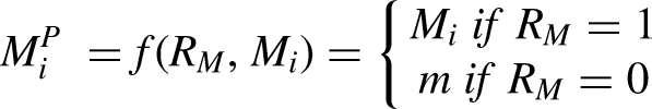
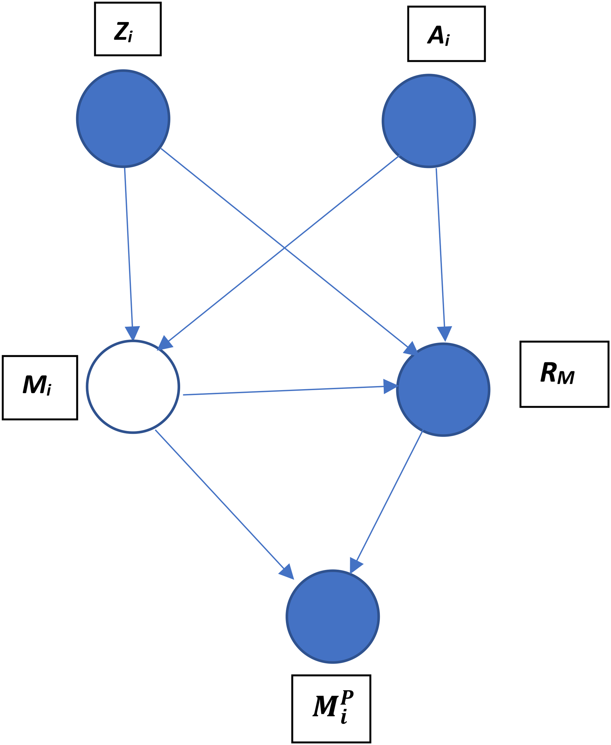
This is a particular case of the generic problem of “missingness” addressed by Mohan and Pearl (2021). Following their approach, Figure 1 illustrates the problem of panel retention in analyzing demographic events using a directed acyclic causal graph when ${\mathit{X}}_{\mathit{i}}$ contains two variables: ${\mathit{X}}_i=[Z_i{A}_i].$ When a person drops out of the panel, a value for $M_i$ is missing and we obtain a missing measurement designated by m. The panel retention process can be modeled using an observed proxy variable $M_i^P$ the values for which are determined by $M_i$ and the “missingness mechanism,” $R_M$ , which takes the following form:

$$M_i^P=f(R_M,M_i)=\{\begin{array}{c}{M}_{i}if{R}_M=1\\ mif{R}_M=0\end{array}$$

Figure 1.

Causal graph with selection on event variable M.

When the person is not retained in the panel, whether an event took place or not is concealed and $R_M=0$ . When we observe the occurrence or absence of the event, $R_M=1$ .

The graph depicted in Figure 1 shows, in the conventional statistical terminology (Little and Rubin 2014), a “not missing at random (NMRA)” process because of the edges linking $M_i$ , $R_M$ , and $M_i^P.$ In words, the process generating missing values on the demographic event variable depends on the event itself. Removing the edge between $M_i$ and $R_M$ would make the process “missing at random (MAR),” which is the assumption made in almost all the statistical literature on multivariate incomplete data. Inclusion of the edge means that $R_M$ is not independent of $M_i$ given ${\mathit{X}}_i=[Z_i{A}_i]$ , and by Theorem 1 of Bareinboim, Tian, and Pearl (2014:2412) this means that “there exists no procedure that would be capable of recovering the distribution from selection bias (without adding assumptions).” Theorem 3 in Mohan and Pearl (2021) expresses the ideas simply. It states that the distribution $P[M_i|Z_i,A_i]$ is not recoverable from the observed data because M and $R_M$ are neighbors.

Let $A_i$ be a variable measured in both the survey data and in external population data, while $Z_i$ is only measured in the longitudinal survey data. In the examples later, $A_i$ is a person’s age. As explained below, the proposed adjustment procedure aims to approximate the recovery of moments of $P[M_i|Z_i,A_i]$ by using external population data on the marginal distribution $P[M_i|A_i]$ . ¹

Application of Bayes Theorem

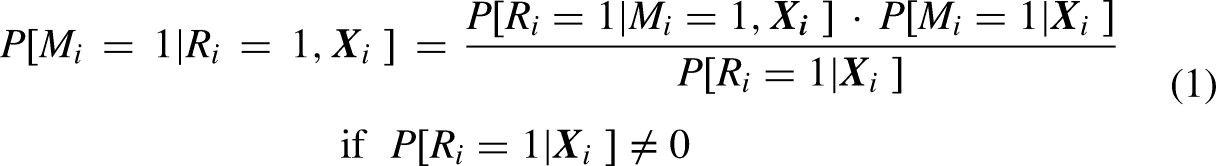
Returning to the general formulation, by Bayes Theorem, we can express the conditional probability as

$$\begin{array}{rl}& P[M_i=1|R_i=1,{\mathit{X}}_i]={\displaystyle \frac{P[R_i=1|M_i=1,{\mathit{X}}_{\mathit{i}}]\cdot P\left[M_i=1|{\mathit{X}}_i\right]}{P\left[R_i=1|{\mathit{X}}_i\right]}}\\ & \mathrm{if}P[R_i=1|{\mathit{X}}_i]\ne 0\end{array}$$

(1)

Re-arranging terms, we obtain

$$P[M_i=1|{\mathit{X}}_i]={\displaystyle \frac{P[M_i=1|R_i=1,{\mathit{X}}_i]\cdot P[R_i=1|{\mathit{X}}_i]}{P[R_i=1|M_i=1,{\mathit{X}}_i]}}$$

(2)

Define $q_i=\frac{P[R_i=1|M_i=0,{\mathit{X}}_i]}{P[R_i=1|M_i=1,{\mathit{X}}_i]}$ , and note that

$$P[R_i=1|{\mathit{X}}_i]=P[R_i=1|M_i=1,{\mathit{X}}_i]\cdot P[M_i=1|{\mathit{X}}_i]$$

$$+P[R_i=1|M_i=0,{\mathit{X}}_{\mathit{i}}]\cdot (1-P[M_i=1|{\mathit{X}}_i]).$$

From these definitions, equation (2) entails the key equation for the analysis, which follows:

$$P[M_i=1|{\mathit{X}}_i]={\displaystyle \frac{P[M_i=1|R_i=1,{\mathit{X}}_i]q_i}{1-P[M_i=1|R_i=1,{\mathit{X}}_i](1-q_i)}}$$

(3)

If, conditional on ${\mathit{X}}_i$ , remaining in the panel to the subsequent wave is independent of the event, then $q_i=1$ and the conditional and unconditional probabilities of the event coincide. It is, however, plausible that if the event is, for example, residential mobility, $q_i$  > 1 because it is more difficult to follow people in the panel when they move. ²

If $q_i>1(q_i<1),$ the denominator of equation (3) is smaller (larger) than $q_i$ . ³ This implies that the unconditional probability of the event given ${\mathit{X}}_i$ is a multiple (fraction) of the conditional probability given ${\mathit{X}}_i$ . If we were able to obtain an estimate of $q_i$ from external data, then the right-hand side of (3) involves only observable variables.

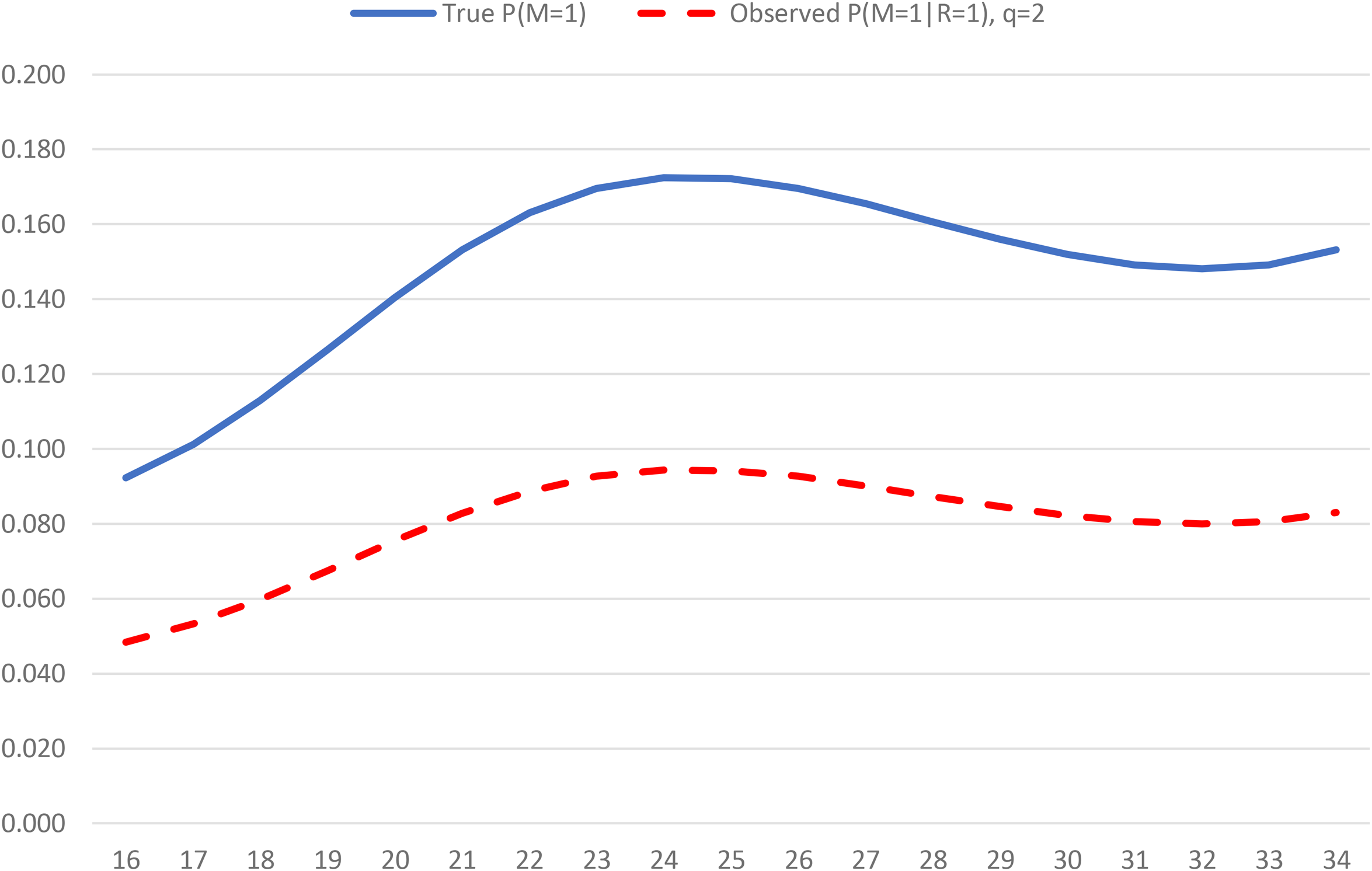
Figure 2 plots a hypothetical age profile of true event probabilities $(P[M_i=1|age])$ , along with the probabilities conditional on retention $(P[M_i=1|R_i=1,age])$ , which is calculated using equation (3) under the assumption that $q_i=2$ for everyone and denoted as “observed.” It clearly deviates substantially from $P[M_i=1|age]$ .

Figure 2.

Event (M = 1) probabilities by age: Hypothetical true and observed (conditional on panel retention), q = 2.

The Adjustment Procedure

The adjustment of conditional probabilities to obtain unconditional ones amounts to choosing values for $q_i$ estimated from external population information. The adjustment procedure proposed obtains an estimate of a “weighted average” of the $q_i,\mathrm{denoted}$ $\hat{q}$ , either globally or for discrete groups (e.g., gender or time period). Let ${\mathit{X}}_i=[{\mathit{Z}}_{\mathit{i}}{A}_i],\mathrm{where}$ $A_i$ is a scalar measured in both the survey and the external population data and the marginal distribution $P[M_i|A_i]$ is observed in the external data. The estimate of $\hat{q}$ is obtained by substituting $P[M_i|A_i]$ for $P[M_i|{\mathit{X}}_{\mathit{i}}]$ and $P[M_i|R_i=1,A_i]$ for $P[M_i|R_i=1,{\mathit{X}}_{\mathit{i}}]$ in equation (3) and estimating $\hat{q}$ using non-linear least squares over discrete categories of $A_i.$ ⁴ $\hat{q}$ is a measure of how close the unconditional probability is to its conditional estimate. The estimate of the unconditional probability of the event is then obtained by substituting $\hat{q}$ in the original equation (3) and it is denoted as ${\hat{P}}_M[{\mathit{Z}}_{\mathit{i}},A_i,\hat{q}](={\hat{P}}_{Mi}$ for short).

Marginal Effects of Covariates on Unconditional Probabilities

This section considers the adjustment of marginal effects in a parametric model with continuous covariates. ⁵ The unconditional marginal effect for element j of ${\mathit{X}}_{\mathit{i}}$ is given by $\frac{dP[M=1|{\mathit{X}}_{\mathit{i}}]}{d{X}_{ij}}=UM{E}_{ij}$ and the conditional one as $\frac{dP[M=1|R=1,{\mathit{X}}_{\mathit{i}}]}{d{X}_{ij}}=CM{E}_{ij}$ . If we assume $q_i=\hat{q}$ , then from equation (3), we obtain an estimate of $UM{E}_{ij}$ :

$$\widehat{UM{E}_{ij}}={\displaystyle \frac{\hat{q}{\widehat{CME}}_{ij}}{{[1-\hat{P}[M_i=1|R_i=1,{\mathit{X}}_{\mathit{i}}](1-\hat{q})]}^2}}$$

(4)

The ratio $\frac{\widehat{UM{E}_{ij}}}{\widehat{CM{E}_{ij}}}$ exceeds (is less than) unity for $\hat{q}>1(\hat{q}<1)$ . In a parametric model of an event with normally distributed errors, the marginal effects are the product of the relevant probit slope parameter estimate and the Normal density function evaluated using all the parameter estimates (including the intercept) and an individual's ${\mathit{X}}_{\mathit{i}}$ values. The mean $\widehat{UM{E}_{ij}}$ in the selected data, $E[{\widehat{UME}}_{ij}|R_i=1],$ differs from the true mean unconditional marginal effect, $E[UM{E}_{ij}]$ , for three reasons: (1) because of errors in estimating $CM{E}_{ij}$ ; (2) because of using $\hat{q}$ for everyone and (3) because of the difference in the distribution of ${\mathit{X}}_i$ in the selected data from that in the entire population. The last reason is addressed, at least approximately, by reweighting the data, as explained in the next section and illustrated with artificial data in the section “Artificial Data.”

Illustrative Structural Model

Consider the following model, in which panel retention $(R_i=1)$ is influenced by (a) the event occurring ( $M_i=1$ ) and/or by (b) correlation between omitted factors influencing the event and panel retention ( $u_i$ and ${\epsilon }_i$ respectively):

$$M_i^{*}={\beta }_0+\mathit{\beta }{\mathit{X}}_i+u_i$$

(5a)

$$R_i^{*}={\alpha }_0+\alpha M_i+\mathit{\gamma }{\mathit{X}}_i+{\epsilon }_i$$

(5b)

where $u_i$ and ${\epsilon }_i$ are distributed as joint standard Normal and $\mathrm{E}\left[{\mathit{X}}_i{u}_i\right]=0=\mathrm{E}\left[{\mathit{X}}_i{\epsilon }_i\right].$ In the data, we only observe cases for which $R_i=1,\mathrm{which}\mathrm{occurs}\mathrm{when}{R}_i^{*}>0$ . The event occurs ( $M_i=1$ ) when $M_i^{*}>0.$ The biases that arise because of conditioning on retention can be most easily illustrated when $\alpha =0$ .

Form the expectation for the latent index $M_i^{*}$ associated with the event conditional on panel retention:

$$E(M_i^{*}|{\mathit{X}}_i,R_i=1)={\beta }_0+\mathit{\beta }{\mathit{X}}_i+E(u_i|{\alpha }_0+\mathit{\gamma }{\mathit{X}}_i+{\epsilon }_i>0)={\beta }_0+\mathit{\beta }{\mathit{X}}_i+E(u_i|{\epsilon }_i>-{\alpha }_0-\mathit{\gamma }{\mathit{X}}_i)$$

(6)

If $\mathrm{\Phi }({\alpha }_0+\mathit{\gamma }{\mathit{X}}_i)$ is the standard Normal distribution function and $\varphi ({\alpha }_0+\mathit{\gamma }{\mathit{X}}_i)$ is the standard Normal density function it follows from the statistics of truncated Normal distributions that

$$E(M_i^{*}|{\mathit{X}}_i,R_i=1)={\beta }_0+\mathit{\beta }{X}_i+\rho \left[{\displaystyle \frac{\varphi ({\alpha }_0+\mathit{\gamma }{\mathit{X}}_i)}{\mathrm{\Phi }({\alpha }_0+\mathit{\gamma }{\mathit{X}}_i)}}\right]$$

(7)

where $\rho$ is the correlation coefficient between u and $\epsilon$ . ⁶ The ratio in brackets is often called the inverse Mills ratio or “Heckman's lambda” (Heckman 1979). It is a monotone decreasing function of the probability that an observation is selected into the sample, $\mathrm{\Phi }({\alpha }_0+\mathit{\gamma }{\mathit{X}}_i).$ It follows that if $\rho$ is non-zero, then $E(M_i^{*}|{\mathit{X}}_i,R_i=1)\ne {\beta }_0+\mathit{\beta }{\mathit{X}}_{\mathit{i}}.$ If, for example, $\rho <0$ , then $E(M_i^{*}|{\mathit{X}}_i,R_i=1)<{\beta }_0+\mathit{\beta }{\mathit{X}}_i$ ; that is, the event is less likely in the selected sample than in the general population. In terms of $q_i,q_i>1$ when $\rho <0$ , and $q_i<1$ when $\rho >0$ . Thus, the parameter estimates are a function of $\mathit{\gamma }$ when $\rho$ is non-zero.

The estimated impact of the jth element of ${\mathit{X}}_i$ , $X_{ij},$ on the latent index $M_i^{*}$ is also biased when $\rho \ne 0$ and ${\gamma }_j\ne 0.$ It confuses the impact of $X_{ij}$ on $M_i^{*}$ , which affects the probability of the event, with its impact on panel retention. To see this, consider the impact of $X_{ij}$ on the conditional expectation of $M_i^{*}.$ From equation (7), if ${\gamma }_j>0\mathrm{and}\rho <0$ , then in the limit the estimate of ${\beta }_j$ converges to the mean of $\frac{d(M_i^{*}|{\mathit{X}}_{\mathit{i}},R_i=1)}{d{X}_{ij}}>{\beta }_j.$ The inequality arises because higher $X_{ij}$ increases the probability of retention and lowers the inverse Mills ratio, and the opposite inequality obtains if ${\gamma }_j<0\mathrm{and}\rho <0$ . In other words, the estimate of ${\beta }_j$ from a probit model from the selected sample will tend to be biased in the direction of the sign of ${\gamma }_j\mathrm{when}\rho <0$ . Similarly, if ${\gamma }_j<0\mathrm{and}\rho >0$ , then the estimate of ${\beta }_j$ converges to the mean of $\frac{d(M_i^{*}|{\mathit{X}}_{\mathit{i}},R_i=1)}{d{X}_{ij}}>{\beta }_j$ and the opposite inequality obtains when ${\gamma }_j>0\mathrm{and}\rho >0$ . Thus, the estimate of ${\beta }_j$ from the selected sample will tend to be biased in the opposite direction to the sign of ${\gamma }_j\mathrm{when}\rho >0.$

The estimate of ${\beta }_j$ is also correlated with the estimate of ${\beta }_0$ , which is biased downward (upward) when $\rho <0(>0).$ Because of this correlation, the estimate of ${\beta }_j$ can be biased even when ${\gamma }_j=0.$

The marginal effect of $X_{ij}$ on the probability of the event is ${\beta }_j\varphi ({\beta }_0+\mathit{\beta }{\mathit{X}}_i)$ . The estimated average marginal effect from the selected sample will differ from its true value because of bias in estimating $\mathit{\beta }$ and ${\beta }_0\mathrm{and}$ because of the difference in the distribution of ${\mathit{X}}_{\mathit{i}}$ in the selected data from that in the entire population, which depends on $\mathit{\gamma }$ . The last issue can be addressed by re-weighting the data in the computation of the mean value of ${\beta }_j\varphi ({\beta }_0+\mathit{\beta }{\mathit{X}}_i)$ . In the illustrative model here with $\alpha =0$ , we can obtain consistent estimates of ${\alpha }_0$ and $\mathit{\gamma }$ by estimating a probit model for $P[R_i=1|{\mathit{X}}_i]$ , and from these parameter estimates, we obtain an estimate of the “propensity score” for panel retention, $\hat{P}[R_i=1|{\mathit{X}}_i]$ . The weights for the computation of the average marginal effects are then 1/ $\hat{P}[R_i=1|{\mathit{X}}_i]$ .

Artificial Data

Discussion of Figure 1 indicated that there is no procedure that can produce consistent estimates of the parameters of equation (5a) when $\alpha \ne 0\mathrm{or}\rho \ne 0$ , because in either of these cases $M_i$ and $R_M$ are neighbors. That is, we cannot recover $P[M_i=1|{\mathit{X}}_i]$ from $P[M_i=1|{\mathit{X}}_i,R_i=1]$ . Simulations of parameter estimation, reweighting, and application of the adjustment procedure using $\hat{q}$ can help us understand better how well the adjustment works when there are “departures from recoverability.”

The simulations use the following variant of the structural model in the section “Illustrative Structural Model” in which ${\mathit{X}}_i=[Z_i{A}_i]$ , with both $Z_i\mathrm{and}{A}_i$ being scalars:

$$M_i*={\beta }_0+{\beta }_a{A}_i+{\beta }_z{Z}_i+u_i$$

(5a\prime)

$$R^{*}={\alpha }_0+\alpha M_i+{\gamma }_a{A}_i+{\gamma }_z{Z}_i+{\epsilon }_i,\alpha \le 0$$

(5b\prime)

The variable $A_i$ is assumed to be available in the external population data from which we obtain estimates of the marginal distribution $P[M_i=1|A_i]$ for the entire population. The focus of the discussion is on the marginal effect of $Z_i$ on $P[M_i=1|A_i,Z_i]$ because the most important reason for using the survey data is the availability of measures of key variables which are not in the external data for which we would like to estimate their unconditional marginal effects on the event. The marginal effect of $A_i$ conditional on $Z_i$ may also differ from its association with $M_i$ in the marginal distribution. In the simulations which follow the true values of the parameters in equation $(5{\mathrm{a}}^{\mathrm{\prime }})$ are taken to be ${\beta }_a=1,{\beta }_z=0.5,{\beta }_0=-1.28$ and ${\alpha }_0=0.5$ in all analyses.

“Small Departures” from Recoverability

First consider the case in which $\rho =\alpha =0$ , which amounts to removing the edge between $M_i$ and $R_M$ in Figure 1. We know that $P[M_i|Z_i,A_i]$ is recoverable in this case. In particular, we can recover the mean $P[M_i=1|Z_i,A_i]$ and the average marginal effect of $Z_i$ on $P[M_i|Z_i,A_i]$ by reweighting the conditional sample (i.e., conditional on $R_i=1$ ) using the inverse of $\hat{P}[R_i|Z_i,A_i]$ as the weight in the mean calculations (i.e., inverse propensity score weighting).

To illustrate the impact of departures from $\rho =\alpha =0$ consider simulations of parameter estimation in variants of the model in $(5{\mathrm{a}}^{\mathrm{\prime }})\mathrm{and}(5{\mathrm{b}}^{\mathrm{\prime }})$ with continuous $A_i$ and $Z_i$ which are drawn from a joint standard Normal distribution with correlation coefficient $r_{az}$ . The exposition creates large illustrative data sets of 100,000 observations under different parameter assumptions to see how the estimated mean probability of an event and of the mean effect of a covariate on it from a sample conditioned on retention differs from their true values and how well adjustment remedies the difference. ⁷ The variants of the model are illustrated for different impacts of $A_i$ and $Z_i$ on the latent variable for panel retention $({\gamma }_a\mathrm{and}{\gamma }_z)$ . Let mean[.] indicate the sample mean.

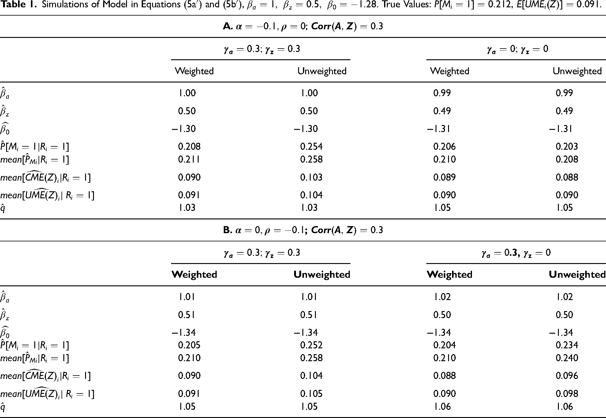
To illustrate how well reweighting and adjustment using an estimate of $\hat{q}$ works in this context, first assume that $\alpha =-0.1,\rho =0\mathrm{and}{r}_{az}=0.3$ . When $\alpha \ne 0$ we must work with a mis-specified function for the probability of panel retention which omits $M_i$ , and contains only $Z_i\mathrm{and}{A}_i$ , and so the re-weighting can only be approximate. Comparison of the two columns for each of the two-parameter configurations in panel A of Table 1 ( ${\gamma }_a={\gamma }_z=0.3$ and ${\gamma }_a={\gamma }_z=0$ ) indicates that reweighting alone makes the mean estimated conditional probability of the event and the average conditional marginal effect of $Z_i$ much closer to their unconditional true counterparts (0.212 and 0.091, respectively), because reweighting takes account of the different distribution of $Z_i\mathrm{and}{A}_i$ in the sample which conditions on panel retention. As we would expect, the reweighting is much more important when ${\gamma }_a={\gamma }_z=\mathrm{0.3.}$

Table 1.

Simulations of Model in Equations (5a′) and (5b′), ${\beta }_a=1,{\beta }_z=0.5,{\beta }_0=-1.28$ . True Values: $P[M_i=1]=0.212$ , $E[UM{E}_i(Z)]=0.09$ 1.

A. $\mathit{\alpha }=-0.1,\mathit{\rho }=0$ ; $\mathit{C}\mathit{o}\mathit{r}\mathit{r}(\mathit{A},\mathit{Z})=0.3$
	${\mathit{\gamma }}_{\mathit{a}}=0.3;{\mathit{\gamma }}_{\mathit{z}}=0.3$		${\mathit{\gamma }}_{\mathit{a}}=0;{\mathit{\gamma }}_{\mathit{z}}=0$
	Weighted	Unweighted	Weighted	Unweighted
${\hat{\beta }}_a$	1.00	1.00	0.99	0.99
${\hat{\beta }}_z$	0.50	0.50	0.49	0.49
$\widehat{{\beta }_0}$	−1.30	−1.30	−1.31	−1.31
$\hat{P}[M_i=1|R_i=1]$	0.208	0.254	0.206	0.203
$mean[{\hat{P}}_{Mi}|R_i=1]$	0.211	0.258	0.210	0.208
mean[ $\widehat{CME}(Z{)}_i|R_i=1$ ]	0.090	0.103	0.089	0.088
$mean[{\widehat{UME(Z)}}_i|R_i=1]$	0.091	0.104	0.090	0.090
$\hat{q}$	1.03	1.03	1.05	1.05
B. $\mathit{\alpha }=0,\mathit{\rho }=-0.1$ ; $\mathit{C}\mathit{o}\mathit{r}\mathit{r}(\mathit{A},\mathit{Z})=0.3$
	${\mathit{\gamma }}_{\mathit{a}}=0.3;{\mathit{\gamma }}_{\mathit{z}}=0.3$		${\mathit{\gamma }}_{\mathit{a}}=0$ .3, ${\mathit{\gamma }}_{\mathit{z}}=0$
	Weighted	Unweighted	Weighted	Unweighted
${\hat{\beta }}_a$	1.01	1.01	1.02	1.02
${\hat{\beta }}_z$	0.51	0.51	0.50	0.50
$\widehat{{\beta }_0}$	−1.34	−1.34	−1.34	−1.34
$\hat{P}[M_i=1|R_i=1]$	0.205	0.252	0.204	0.234
$mean[{\hat{P}}_{Mi}|R_i=1]$	0.210	0.258	0.210	0.240
mean[ $\widehat{CME}(Z{)}_i|R_i=1$ ]	0.090	0.104	0.088	0.096
$mean[{\widehat{UME(Z)}}_i|R_i=1]$	0.091	0.105	0.090	0.098
$\hat{q}$	1.05	1.05	1.06	1.06

Assume that population data on the unconditional marginal probability $P[M_i=1|A_i]$ is available for deciles of $A_i$ , labeled $A_i^D.$ For example, with the parameter configuration in the left-hand side of panel A, $q_i$ decreases with $A_i$ . In the lowest decile, $E[q_i|A_i^D=1]=1.10$ and in the highest $E[q_i|A_i^D=10]=\mathrm{1.03.}$ We estimate $\hat{q}$ by relating $P[M_i=1|A_i^D]$ to $\hat{P}[M_i=1|R_i=1,A_i^D]$ in equation (3) using non-linear least squares over deciles of $X_i$ . Because the difference between these two quantities is larger for the higher deciles, these attract more weight in the non-linear least squares’ estimator, yielding an estimate of $\hat{q}$ of 1.03 (robust SE = 0.001). Using $\hat{q}$ to adjust the reweighted estimates of the mean probability of the event and of the average marginal effect of $Z_i$ moves the estimates closer to their true values.

When ${\gamma }_a={\gamma }_z=0$ (right-hand side of panel A) the estimates of the impacts of $A_i$ and $Z_i$ in the mis-specified propensity score equation (not shown) are spuriously negative (rather than 0), reflecting that $\alpha <0$ in the true retention equation. ⁸ Yet the re-weighting and adjustment using $\hat{q}$ works relatively well in estimating the mean probability of the event and the average marginal effect of $Z_i$ , although not as close as in parameter configuration on the left-hand side of panel A.

Next consider the case in which $\rho =-0.1\mathrm{and}\alpha =0$ which also represents a small departure from recoverability. In this case, the estimates of parameters of the propensity score equation are consistent. Similar conclusions concerning reweighting and adjustment using $\hat{q}$ apply (see panel B of Table 1). Thus, small departures from recoverability can be addressed well by re-weighting and the proposed adjustment procedure. The next section considers how well reweighting and adjustment using $\hat{q}$ works for large departures from recoverability.

“Large Departures” From Recoverability

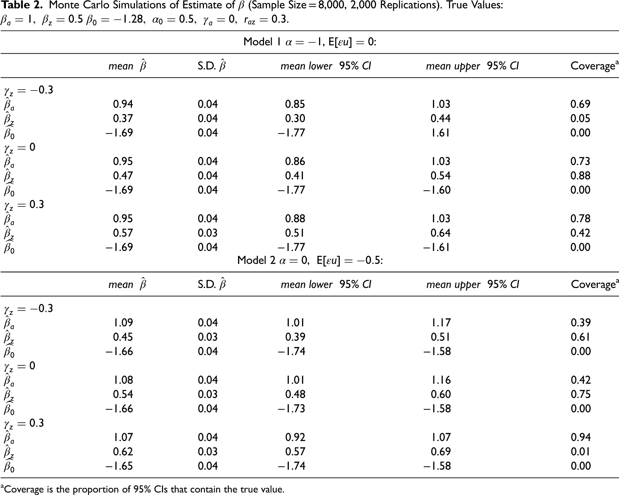
As in the previous section, $A_i$ and $Z_i$ are continuous and are drawn from a joint standard Normal distribution with correlation coefficient $r_{az}.$ We consider simulations of parameter estimation in two variants of the model in $(5{\mathrm{a}}^{\mathrm{\prime }})\mathrm{and}(5{\mathrm{b}}^{\mathrm{\prime }})$ , which represent relatively strong mechanisms of selection related to event outcomes. In one model the event directly affects retention (Model 1): $\alpha =-1$ , $\rho =0$ . In the other, the association between retention and the event is assumed to be due solely to omitted variables that are associated with both processes (Model 2): $\alpha =0$ , $\rho =-0.5$ .

First consider how parameter estimation on the conditional sample is affected by strong departures from recoverability in these two models. Monte Carlo simulations of the estimate of the probit parameters ( ${\beta }_0$ , ${\beta }_a$ , and ${\beta }_z$ ) using samples of 8,000 cases are shown in Table 2. In these, the impact of $A_i$ on retention ( ${\gamma }_a$ ) is set to zero, $r_{az}=0.3$ and ${\gamma }_z$ is varied between −0.3 and 0.3. What is most striking is that the 95% confidence interval of the estimate of the intercept ${\beta }_0$ never contains its true value (−1.28), creating substantial downward bias in an estimate of the mean probability of the event from the selected sample. Also, the 95% confidence interval for the slope parameters ${\beta }_a$ and ${\beta }_z$ generally includes its true value much less than 95% of the time, and in some parameter configurations almost never includes its true value. Not surprisingly the estimate of ${\beta }_z\mathrm{performs}\mathrm{best}\mathrm{when}{\gamma }_z=0.$ Estimates of these parameters may be considered of less intrinsic interest on their own than estimates of the average marginal effects of $Z_i$ and $A_i.$ Even after reweighting using the inverse propensity score, these are affected by bias in estimating both the intercept and slope parameters of the probit model. The focus now shifts to these quantities.

Table 2.

Monte Carlo Simulations of Estimate of $\beta$ (Sample Size = 8,000, 2,000 Replications). True Values: ${\beta }_a=1,{\beta }_z=0.5{\beta }_0=-1.28,{\alpha }_0=0.5,{\gamma }_a=0,r_{az}=0.3$ .

Model 1 $\alpha =-1$ , $\mathrm{E}[\epsilon u]=0$ :
	$mean$ $\hat{\beta }$	S.D. $\hat{\beta }$	$meanlower$ $95\text{\%}CI$	$meanupper$ $95\text{\%}CI$	Coverage a
${\gamma }_z=-0.3$
${\hat{\beta }}_a$	0.94	0.04	0.85	1.03	0.69
${\hat{\beta }}_z$	0.37	0.04	0.30	0.44	0.05
$\widehat{{\beta }_0}$	−1.69	0.04	−1.77	1.61	0.00
${\gamma }_z=0$
${\hat{\beta }}_a$	0.95	0.04	0.86	1.03	0.73
${\hat{\beta }}_z$	0.47	0.04	0.41	0.54	0.88
$\widehat{{\beta }_0}$	−1.69	0.04	−1.77	−1.60	0.00
${\gamma }_z=0.3$
${\hat{\beta }}_a$	0.95	0.04	0.88	1.03	0.78
${\hat{\beta }}_z$	0.57	0.03	0.51	0.64	0.42
$\widehat{{\beta }_0}$	−1.69	0.04	−1.77	−1.61	0.00

Model 2 $\alpha =0$ , $\mathrm{E}[\epsilon u]=-0.5$ :
	$mean$ $\hat{\beta }$	S.D. $\hat{\beta }$	$meanlower$ $95\text{\%}CI$	$meanupper$ $95\text{\%}CI$	Coverage a
${\gamma }_z=-0.3$
${\hat{\beta }}_a$	1.09	0.04	1.01	1.17	0.39
${\hat{\beta }}_z$	0.45	0.03	0.39	0.51	0.61
$\widehat{{\beta }_0}$	−1.66	0.04	−1.74	−1.58	0.00
${\gamma }_z=0$
${\hat{\beta }}_a$	1.08	0.04	1.01	1.16	0.42
${\hat{\beta }}_z$	0.54	0.03	0.48	0.60	0.75
$\widehat{{\beta }_0}$	−1.66	0.04	−1.73	−1.58	0.00
${\gamma }_z=0.3$
${\hat{\beta }}_a$	1.07	0.04	0.92	1.07	0.94
${\hat{\beta }}_z$	0.62	0.03	0.57	0.69	0.01
$\widehat{{\beta }_0}$	−1.65	0.04	−1.74	−1.58	0.00

^aCoverage is the proportion of 95% CIs that contain the true value.

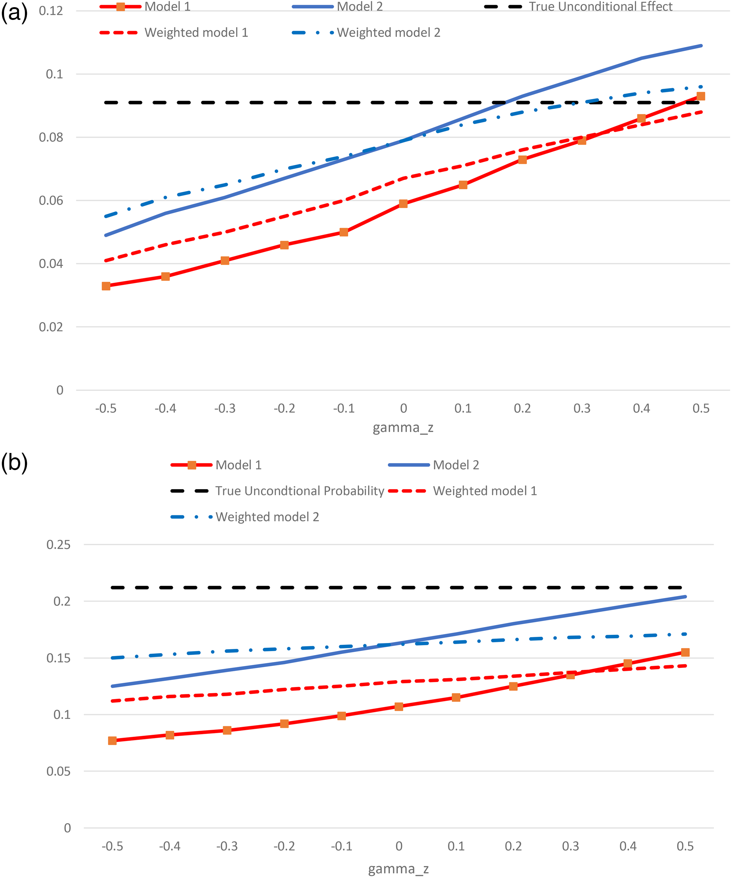
It is informative to see how the conditional probability of the event and conditional marginal effect of $Z_i$ and vary with ${\gamma }_z.$ As in Table 1, the analysis creates large illustrative data sets of 100,000 observations each under different parameter assumptions. Figures 3A and 3B illustrate how $mean[{\widehat{CME}}_i(Z)|R_i=1])$ and $mean\left[\hat{P}\right[M_i=1|R_i=1]$ , respectively, vary with ${\gamma }_z$ when ${\gamma }_a=0\mathrm{and}{r}_{az}=0.3$ . There is an approximately linear relationship between ${\gamma }_z$ and these conditional quantities which is the same in both models but with higher mean values for Model 2. After reweighting using the inverse propensity score, the linear relationship between ${\gamma }_z$ and the conditional quantities is less steep. In Figure 3A, the estimator of the reweighted $mean{\widehat{[CME}}_i(Z)|R_i=1]$ approaches the true value as ${\gamma }_z$ increases because of the increase in the estimate of ${\beta }_z$ , which becomes increasingly upward biased beyond ${\gamma }_z=0$ . Because in these two models $\hat{q}>1$ , the adjustment procedure entails that $mean[{\widehat{UME}}_i|R_i=1]>$ $mean{\widehat{[CME}}_i(Z)|R_i=1]$ and so there must be a value of ${\gamma }_z$ for which adjustment using $\hat{q}$ takes us farther from the true value than using the conditional estimate. For instance, in model 2, for ${\gamma }_z>0.3,\mathrm{the}\mathrm{reweighted}$ $mean[{\widehat{CME}}_i(Z)|R_i=1])$ overstates the true marginal effect and adjusting it further upward would only make the estimate worse. In Figure 3B, the reweighted $mean\left[\hat{P}\right[M_i=1|R_i=1]$ remains well below the true value of the unconditional mean.

Figure 3.

(a) Estimated conditional marginal effect of Z and true unconditional effect. (b) Estimated mean conditional and true unconditional probability of the event.

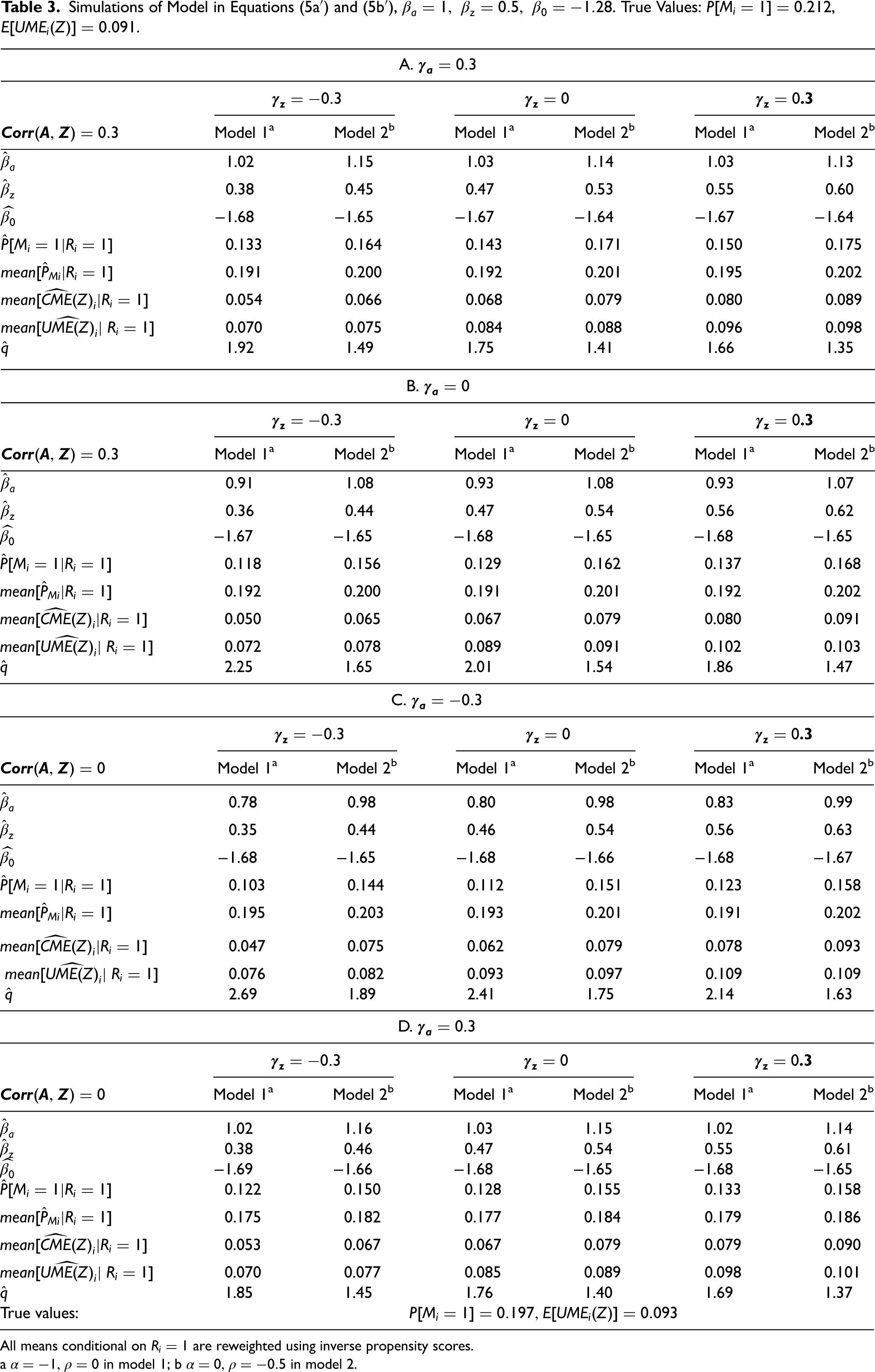
In panels A through C of Table 3, we illustrate nine parameter configurations for each model in which ${\gamma }_a\mathrm{and}{\gamma }_z$ each takes on three possible values: −0.3, 0 and 0.3 and the covariance of A and Z is set to 0.3. In panel D, this covariance is set to 0. Initially, we focus on comparing panels A through C. Amongst these, the adjustment factor $\hat{q}$ is larger in model 1 than model 2; $\hat{q}$ declines with higher values of both ${\gamma }_a\mathrm{and}{\gamma }_z$ , particularly in Model 1, and the decline in $\hat{q}$ is steeper with ${\gamma }_a\mathrm{than}\mathrm{with}{\gamma }_z$ .

Table 3.

Simulations of Model in Equations (5a′) and (5b′), ${\beta }_a=1,{\beta }_z=0.5,{\beta }_0=-1.28$ . True Values: $P[M_i=1]=0.212$ , $E[UM{E}_i(Z)]=0.09$ 1.

A. ${\mathit{\gamma }}_{\mathit{a}}=0.3$
	${\mathit{\gamma }}_{\mathit{z}}=-0.3$		${\mathit{\gamma }}_{\mathit{z}}=0$		${\mathit{\gamma }}_{\mathit{z}}=0$ . 3
$\mathit{C}\mathit{o}\mathit{r}\mathit{r}(\mathit{A},\mathit{Z})=0.3$	Model 1a	Model 2b	Model 1a	Model 2b	Model 1a	Model 2b
${\hat{\beta }}_a$	1.02	1.15	1.03	1.14	1.03	1.13
${\hat{\beta }}_z$	0.38	0.45	0.47	0.53	0.55	0.60
$\widehat{{\beta }_0}$	−1.68	−1.65	−1.67	−1.64	−1.67	−1.64
$\hat{P}[M_i=1|R_i=1]$	0.133	0.164	0.143	0.171	0.150	0.175
$mean[{\hat{P}}_{Mi}|R_i=1]$	0.191	0.200	0.192	0.201	0.195	0.202
mean[ $\widehat{CME}(Z{)}_i|R_i=1$ ]	0.054	0.066	0.068	0.079	0.080	0.089
$mean[{\widehat{UME(Z)}}_i|R_i=1]$	0.070	0.075	0.084	0.088	0.096	0.098
$\hat{q}$	1.92	1.49	1.75	1.41	1.66	1.35

B. ${\mathit{\gamma }}_{\mathit{a}}=0$
	${\mathit{\gamma }}_{\mathit{z}}=-0.3$		${\mathit{\gamma }}_{\mathit{z}}=0$		${\mathit{\gamma }}_{\mathit{z}}=0$ . 3
$\mathit{C}\mathit{o}\mathit{r}\mathit{r}(\mathit{A},\mathit{Z})=0.3$	Model 1a	Model 2b	Model 1a	Model 2b	Model 1a	Model 2b
${\hat{\beta }}_a$	0.91	1.08	0.93	1.08	0.93	1.07
${\hat{\beta }}_z$	0.36	0.44	0.47	0.54	0.56	0.62
$\widehat{{\beta }_0}$	−1.67	−1.65	−1.68	−1.65	−1.68	−1.65
$\hat{P}[M_i=1|R_i=1]$	0.118	0.156	0.129	0.162	0.137	0.168
$mean[{\hat{P}}_{Mi}|R_i=1]$	0.192	0.200	0.191	0.201	0.192	0.202
mean[ $\widehat{CME}(Z{)}_i|R_i=1$ ]	0.050	0.065	0.067	0.079	0.080	0.091
$mean[{\widehat{UME(Z)}}_i|R_i=1]$	0.072	0.078	0.089	0.091	0.102	0.103
$\hat{q}$	2.25	1.65	2.01	1.54	1.86	1.47

C. ${\mathit{\gamma }}_{\mathit{a}}=-0.3$
	${\mathit{\gamma }}_{\mathit{z}}=-0.3$		${\mathit{\gamma }}_{\mathit{z}}=0$		${\mathit{\gamma }}_{\mathit{z}}=0$ . 3
$\mathit{C}\mathit{o}\mathit{r}\mathit{r}(\mathit{A},\mathit{Z})=0$	Model 1a	Model 2b	Model 1a	Model 2b	Model 1a	Model 2b
${\hat{\beta }}_a$	0.78	0.98	0.80	0.98	0.83	0.99
${\hat{\beta }}_z$	0.35	0.44	0.46	0.54	0.56	0.63
$\widehat{{\beta }_0}$	−1.68	−1.65	−1.68	−1.66	−1.68	−1.67
$\hat{P}[M_i=1|R_i=1]$	0.103	0.144	0.112	0.151	0.123	0.158
$mean[{\hat{P}}_{Mi}|R_i=1]$	0.195	0.203	0.193	0.201	0.191	0.202
mean[ $\widehat{CME}(Z{)}_i|R_i=1$ ]	0.047	0.075	0.062	0.079	0.078	0.093
$mean[{\widehat{UME(Z)}}_i|R_i=1]$	0.076	0.082	0.093	0.097	0.109	0.109
$\hat{q}$	2.69	1.89	2.41	1.75	2.14	1.63

D. ${\mathit{\gamma }}_{\mathit{a}}=0.3$
	${\mathit{\gamma }}_{\mathit{z}}=-0.3$		${\mathit{\gamma }}_{\mathit{z}}=0$		${\mathit{\gamma }}_{\mathit{z}}=0$ . 3
$\mathit{C}\mathit{o}\mathit{r}\mathit{r}(\mathit{A},\mathit{Z})=0$	Model 1a	Model 2b	Model 1a	Model 2b	Model 1a	Model 2b
${\hat{\beta }}_a$	1.02	1.16	1.03	1.15	1.02	1.14
${\hat{\beta }}_z$	0.38	0.46	0.47	0.54	0.55	0.61
$\widehat{{\beta }_0}$	−1.69	−1.66	−1.68	−1.65	−1.68	−1.65
$\hat{P}[M_i=1|R_i=1]$	0.122	0.150	0.128	0.155	0.133	0.158
$mean[{\hat{P}}_{Mi}|R_i=1]$	0.175	0.182	0.177	0.184	0.179	0.186
mean[ $\widehat{CME}(Z{)}_i|R_i=1$ ]	0.053	0.067	0.067	0.079	0.079	0.090
$mean[{\widehat{UME(Z)}}_i|R_i=1]$	0.070	0.077	0.085	0.089	0.098	0.101
$\hat{q}$	1.85	1.45	1.76	1.40	1.69	1.37
True values:	$P[M_i=1]=0.197,E[UM{E}_i(Z)]=0.093$

All means conditional on $R_i=1$ are reweighted using inverse propensity scores.

a $\alpha =-1,\rho =0$ in model 1; b $\alpha =0,\rho =-0.5$ in model 2.

If the adjusted estimates of the unconditional quantities based on the reweighted distribution of $A_i$ and $Z_i(\mathrm{i}.\mathrm{e}.,$ $mean[{\hat{P}}_{Mi}|R_i=1]\mathrm{and}$ $mean[{\widehat{UME}}_i|R_i=1])$ are closer to their corresponding true unconditional value than the conditional estimates $(mean\left[\hat{P}\right[M_i=1|R_i=1]$ and mean[ ${\widehat{CME}}_i|R_i=1],$ respectively), the adjustment procedure can be considered to be superior to using the conditional estimates. Among the estimates illustrated in Table 3, there are three cases of Model 2 in which mean[ ${\widehat{CME}}_i|R_i=1]$ is closer to the true value than mean[ ${\widehat{UME}}_i|R_i=1]$ , all of which have ${\gamma }_z=0.3,$ and, perforce, that will also be the case for ${\gamma }_z>\mathrm{0.3.}$ Panel D eliminates the correlation between A and Z, but the conclusions about which estimator of the marginal effect is closer to the true effect are not affected (cf. panels A and D).

Effectiveness of the Adjustment Procedure for Further Variation in Model Specification

Variants of Model 1

This section reports analysis of the estimates of the conditional event probability and average conditional marginal effect along with the estimates of their unconditional counterparts, which use the adjustment procedure. Thirty-six different parameter configurations for the panel retention equation of Model 1 are considered: ${\gamma }_a\mathrm{and}{\gamma }_z$ each take on three possible values (−0.3, 0 and 0.3) and $\alpha$ takes on four possible values (−0.1, −0.5, −0.75 and −1). In all cases, the correlation between A and Z is assumed to be 0.3, and the estimates of the means are reweighted using the inverse propensity score. The results are used to explore further the effectiveness of the adjustment procedure.

In every case, $mean[{\hat{P}}_{Mi}|R_i=1]$ is closer to the true unconditional mean probability then the conditional mean $(mean[\hat{P}[M_i=1|R_i=1])$ . This is not surprising because we have estimated $\hat{q}$ to minimize the distance between the conditional and unconditional marginal probabilities with respect to age. The adjustment of $\hat{P}[M_i=1|R_i=1]$ using $\hat{q}$ partially corrects for the severe downward bias of the estimate of the ${\beta }_0$ from the conditional sample.

Although $mean[{\widehat{UME}}_i|R_i=1])$ is closer to the true unconditional marginal effect than mean[ ${\widehat{CME}}_i|R_i=1]$ in most of the 36 cases, it is not for 6 cases for which ${\gamma }_z=0.3$ and $\alpha <-0.1$ and ${\gamma }_a\le 0.$ In this range of $\alpha$ and ${\gamma }_a,$ this would also be true for ${\gamma }_z>\mathrm{0.3.}$

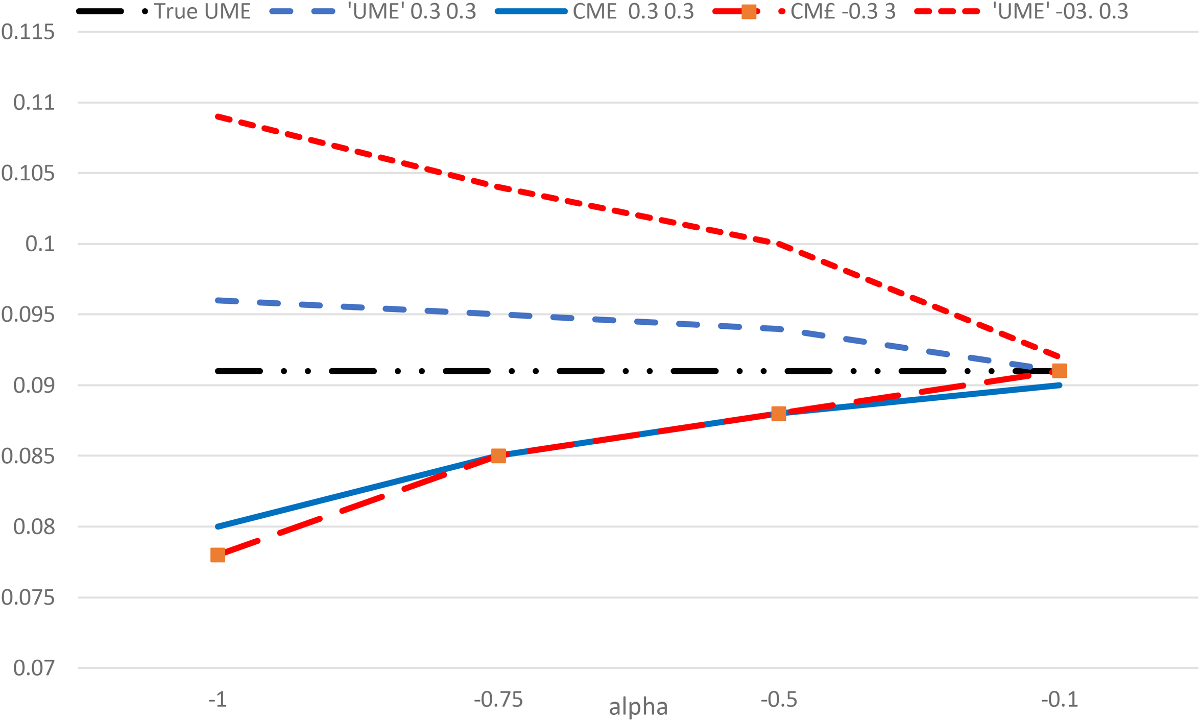
Figure 4 plots the two estimators against different values of $\alpha$ in Model 1 for two sets of gamma parameters: in each ${\gamma }_z=0.3$ while ${\gamma }_a=-0.3\mathrm{or}\mathrm{0.3.}$ Although mean[ ${\widehat{CME}}_i|R_i=1]$ is similar for each set of gamma parameters, the adjustment procedure produces a much larger adjustment factor $\hat{q}$ for the set with ${\gamma }_a=-0.3,$ so that $mean[{\widehat{UME}}_i|R_i=1]$ is farther from the true value than the unadjusted conditional marginal effect in this case and closer to it when ${\gamma }_a=0.3$ . As $\alpha$ declines the downward bias of mean[ ${\widehat{CME}}_i|R_i=1]$ increases (becomes “more negative”), while the adjustment factor $\hat{q}$ increases. The difference between $mean[{\widehat{UME}}_i|R_i=1]$ and mean[ ${\widehat{CME}}_i|R_i=1]$ is the outcome of the “race” between these two factors as $\alpha$ declines.

Figure 4.

Conditional marginal effect of Z and adjusted effect using $\hat{q}$ in Model 1.

Distance is defined as the absolute value of the difference between each estimator and the true value of the average marginal effect of Z. Analysis of the distances in the 36 simulations indicates that the distance for the reweighted mean[ ${\widehat{CME}}_i(Z)|R_i=1]$ declines with increases in the values of $\alpha$ and ${\gamma }_z$ . This is also true for the reweighted $mean[{\widehat{UME}}_i(Z)|R_i=1]$ for which the relationship partly operates through the adjustment factor function $\hat{q}({\gamma }_a,{\gamma }_z,\alpha$ ), which is decreasing in all three panel retention parameters. Although the distances for both estimators decline with increases in ${\gamma }_a$ , their effect on distance is about the same for both.

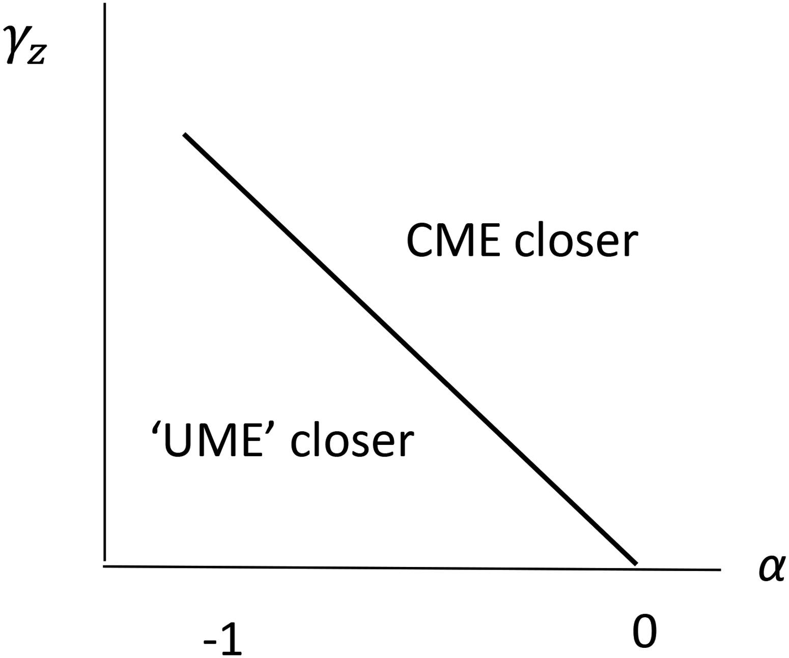
Define the difference between the distances of the two estimators as D, so that they are equidistant when D = 0 and D < 0 indicates that mean[ ${\widehat{CME}}_i(Z)|R_i=1]$ is closer to the true value than $mean[{\widehat{UME}}_i(Z)|R_i=1].$ There is a relationship between $\alpha$ and ${\gamma }_z$ for which D = 0 which is illustrated in Figure 5. Combinations of $\alpha$ and ${\gamma }_z$ above the curve have D < 0, for which mean[ ${\widehat{CME}}_i(Z)|R_i=1]$ is the superior estimator. For any given $\alpha$ , this is more likely to occur when ${\gamma }_z$ is larger. The value of ${\gamma }_a$ has little impact on the position of the $\alpha$ - ${\gamma }_z$ relationship.

Figure 5.

Equidistant estimators’ curve*.

Variants of Model 2

A similar exercise was carried out for variation in ${\gamma }_a,{\gamma }_z\mathrm{and}\rho .$ Again the two gamma parameters take on 3 values each (−0.3, 0 and 0.3) and $\rho$ takes on 3 values: −0.1, −0.25, and −0.5. Among these 27 different parameter configurations for the retention equation, $mean[{\widehat{CME}}_i(Z)|R_i=1]$ is the superior estimator in cases ${\gamma }_z=0.3\mathrm{and}{\gamma }_a=0\mathrm{or}{\gamma }_a=-0.3,$ and this will also be true when ${\gamma }_z>\mathrm{0.3.}$ What emerges is a curve relating $\rho$ and ${\gamma }_z$ along which D = 0, similar to that in Figure 5 for $\alpha$ and ${\gamma }_z$ . ⁹ In this model, a larger value of ${\gamma }_a$ shifts the $\rho$ - ${\gamma }_z$ relationship upward so that for each value of $\rho$ it requires a larger value of ${\gamma }_z$ to make D = 0; put differently, it takes a higher ${\gamma }_z$ to make $mean[{\widehat{CME}}_i|R_i=1]$ the superior estimator. As with Model 1 in relation to $\alpha$ , by biasing the conditional estimates of ${\beta }_z$ upwards by more, a higher ${\gamma }_z$ can offset the downward bias in ${\beta }_z$ caused by a smaller $\rho$ (or $\alpha$ ) thereby producing the same distance from the true marginal effect of Z.

Claims and Conjectures

Of course, there are limits to what we can learn from simulations of variants of a particular model of panel retention like that used above. But there are lessons which aid our understanding of the proposed adjustment procedure. No claim can be made that, even after reweighting, the estimates $mean[{\widehat{UME}}_i|R_i=1]$ and $mean[{\hat{P}}_{Mi}|R_i=1]$ using $\hat{q}$ are consistent estimates of $E[UM{E}_i]$ or mean $P[M_i=1]$ , respectively. But the simulations point to the following conjectures:

The estimator $mean[{\hat{P}}_{Mi}|R_i=1]$ is always closer to the true mean value of $P[M_i=1]$ than $mean[\hat{P}[M_i=1|R_i=1]].$

When the event is weakly associated with panel retention, the two estimators of the marginal effect are very similar and $mean[{\widehat{UME}}_i|R_i=1]$ is usually closer to the true value than $mean[{\widehat{CME}}_i|R_i=1]$ .

When the event is strongly associated with panel retention, $mean[{\widehat{UME}}_i|R_i=1]$ is superior unless the exogenous covariates ( ${\mathit{X}}_i$ ) strongly influence retention in the same direction as they affect M_i.

Information on the direction and strength of the exogenous covariates ( ${\mathit{X}}_i)$ on retention is obtained from estimates of the propensity score equation $\hat{P}[R_i=1|{\mathit{X}}_i],$ and the equation provides weights for calculating means. In the context of the Models 1 and 2, a weak or opposite impact of $Z_i$ on $R_i$ from that on $M_i$ would strongly favor the superiority of $mean[{\widehat{UME}}_i|R_i=1]$ over the simple conditional estimates. In any case, it would be worth reporting both estimators of the unconditional marginal effect: $mean[{\widehat{UME}}_i|R_i=1]$ as well as $mean[{\widehat{CME}}_i|R_i=1]$ .

Examples

In both examples, the survey data is Understanding Society (the UK Household Longitudinal Study). It is a longitudinal survey of the members of approximately 40,000 households in the United Kingdom. Households recruited at the first round of data collection (2009–2011) were visited each year to collect information on changes to their household and individual circumstances. Annual interviews were conducted face-to-face in respondents’ homes by trained interviewers. All members of the households selected at the first wave and their descendants, who become full members of the panel when they reach age 16, constitute the core sample who are followed wherever they move within the UK. All others who join their households in subsequent waves do not become part of the core sample, but they are interviewed as long as they live with at least one core sample member. Thus, the sample is refreshed with younger members annually. Understanding Society is designed to be representative of the UK population at each wave, representing all ages and all educational and social backgrounds (for more details see Understanding Society 2021a, 2021b).

In the residential mobility example, the aim is to estimate the impact of the housing tenure in the household in which a person lives on age-specific movement rates (i.e., the counterpart of Z in the model of the previous section), and in the marriage example, the objective is to estimate the impact of existing children on age-specific marriage rates. In both examples, the external population data has the same target probability as the survey data: the annual age-group specific probability of the event (residential movement or marriage). In Understanding Society, the estimates are based on residential movement (marriage) between annual waves.

Residential Mobility

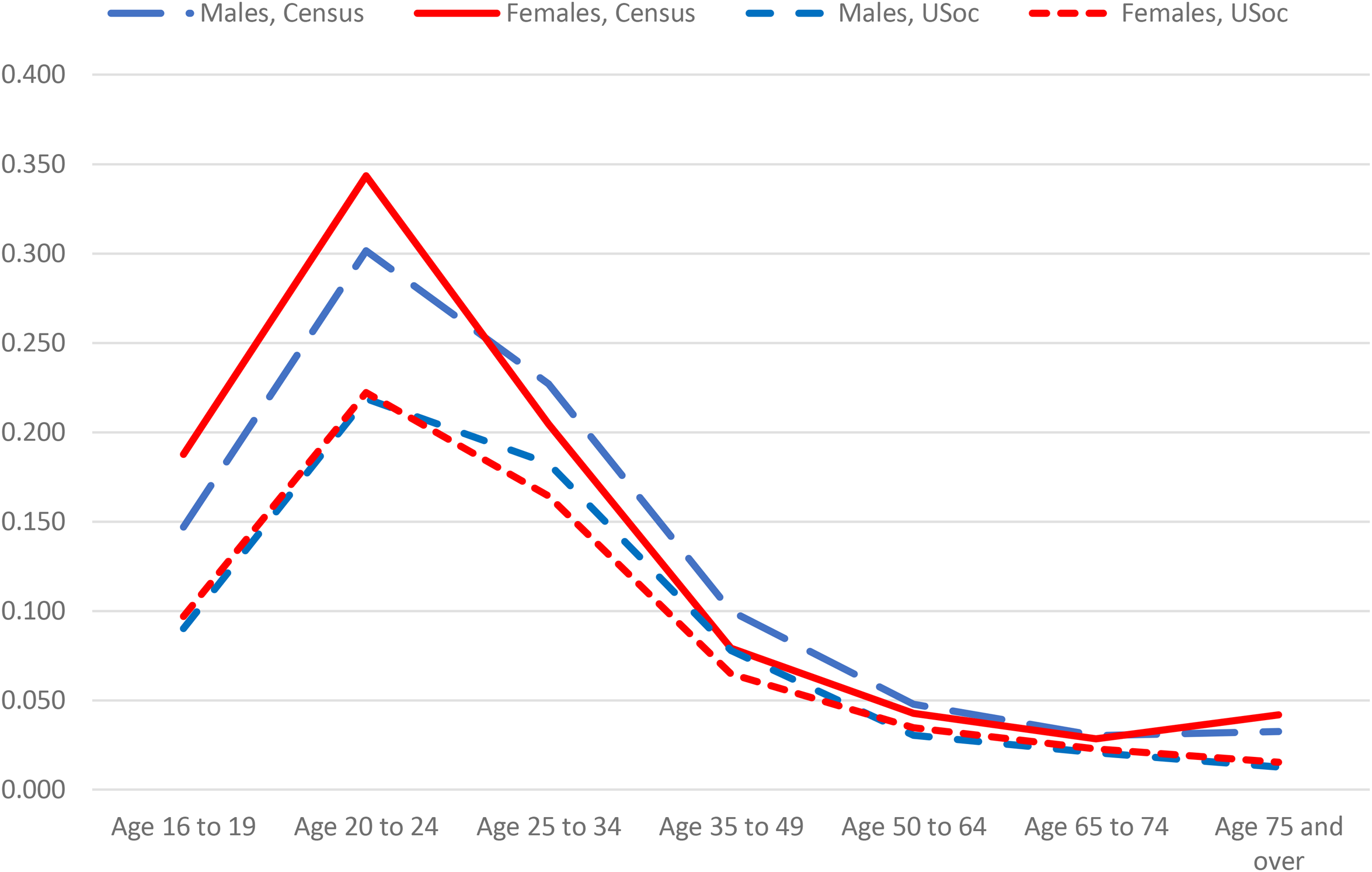
As mentioned often, the study of the probability of moving house is likely to be particularly prone to downward bias from panel attrition. The example uses population data on internal movements within the United Kingdom during the past year derived from the 2011 Census (the last one for which movement data is currently available). Movement is defined as those who were enumerated as having lived elsewhere one year ago within the United Kingdom. The true mobility rate is calculated by dividing this number by the sum of it and the number who lived at the same address in 2011 as one year ago. The rates are computed by sex and age groups and are shown in Figure 6. The corresponding survey data from Understanding Society measures residential mobility as changes in address between their previous annual wave of the survey and the current wave among those interviewed in 2011. These mobility rates are also shown in Figure 6, from which we see that the survey understates mobility among those aged under 50, probably because of larger panel attrition among movers.

Figure 6.

Comparison of Census and Understanding Society internal migration rates 2011.

To estimate $\hat{q}$ , the first step was to estimate the proportion of moving house in the previous year among those interviewed in 2011 in Understanding Society for the seven age groups in Figure 6 for each gender, which are conditional on panel retention. Next, perform non-linear least squares estimation of equation (3) over these seven observations. For men, we estimate $\hat{q}$ to be 1.47 (SE = 0.08) and for women 1.64 (SE = 0.17). ¹⁰

Because our estimate of $P[M_i=1|R_i=1,agegroup]$ from the survey data is subject to sampling error, estimating equation (3) may produce errors-in-variables bias in $\hat{q}$ . It is therefore preferable to apply non-linear least squares to equation $(3^{\mathrm{\prime }})$ which arises from re-writing equation (3):

$$P[M_i=1|R_i=1,{\mathit{X}}_{\mathit{i}}]]={\displaystyle \frac{P[M_i=1|{\mathit{X}}_{\mathit{i}}]}{q_i+P[M_i=1|{\mathit{X}}_{\mathit{i}}](1-q_i)}}$$

(3^\prime)

Using this approach for men, $\hat{q}$ was estimated to be 1.48 (SE = 0.07) and for women 1.70 (SE = 0.16). If the true annual sex- and age-specific mobility rates can be assumed to be the same over the decade 2011–2021 as in 2011, we can compare the 2011 Census mobility rates with mobility rates calculated by pooling all 11 waves of Understanding Society. The estimates of $\hat{q}$ are then 1.46 (SE = 0.15) for men and 1.54 (SE = 0.21) for women. To be conservative, these are the ones used in the adjustment procedure, but there are clearly relatively wide confidence intervals around these estimates.

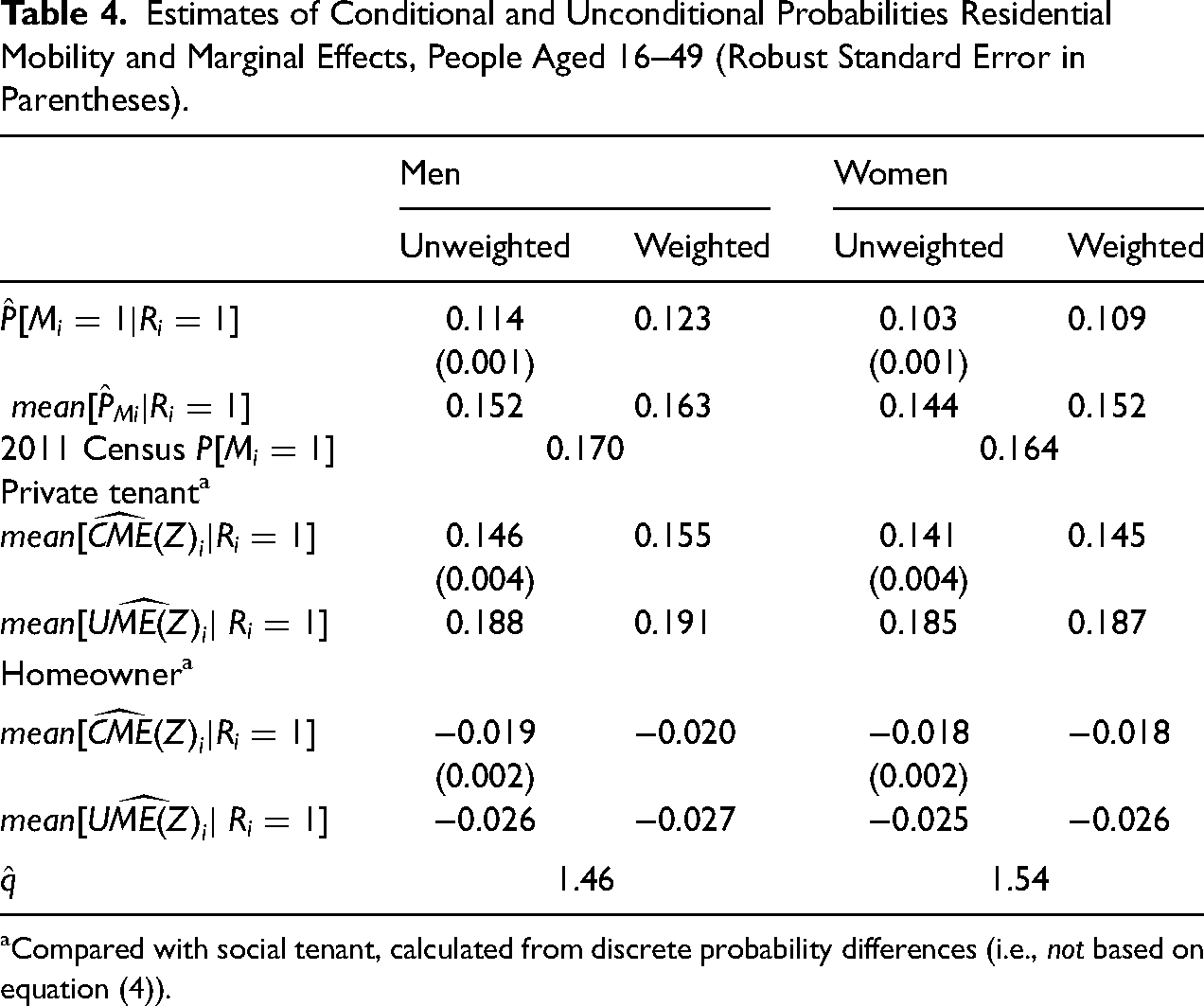
A probit model for residential mobility was estimated using all eleven waves of data (i.e., up to ten pairs of waves) among persons aged 17–49. In the model, mobility depends on a cubic in age, highest educational level, housing tenure (private rental and homeowner cf. social tenancy), an interaction between gender and the presence of a partner (all measured in the previous year) and interview year. In broad terms, the model is similar to those estimated for the UK in Ermisch and Mulder (2019) and Ermisch and Steele (2016). The discussion focuses on the mean probability of the event and the average marginal effect of a person's housing tenure (i.e., treated as Z in the section “Artificial Data”) on the probability of mobility. Table 4 shows the conditional probabilities and marginal effects estimated from the model along with the corresponding estimates of their unconditional counterparts using the adjustment procedure.

Table 4.

Estimates of Conditional and Unconditional Probabilities Residential Mobility and Marginal Effects, People Aged 16–49 (Robust Standard Error in Parentheses).

	Men		Women
	Unweighted	Weighted	Unweighted	Weighted
$\hat{P}[M_i=1|R_i=1]$	0.114 (0.001)	0.123	0.103 (0.001)	0.109
$mean[{\hat{P}}_{Mi}|R_i=1]$	0.152	0.163	0.144	0.152
2011 Census $P[M_i=1$ ]	0.170		0.164
Private tenanta
mean[ $\widehat{CME}(Z{)}_i|R_i=1$ ]	0.146 (0.004)	0.155	0.141 (0.004)	0.145
$mean[{\widehat{UME(Z)}}_i|R_i=1]$	0.188	0.191	0.185	0.187
Homeownera
mean[ $\widehat{CME}(Z{)}_i|R_i=1$ ]	−0.019 (0.002)	−0.020	−0.018 (0.002)	−0.018
$mean[{\widehat{UME(Z)}}_i|R_i=1]$	−0.026	−0.027	−0.025	−0.026
$\hat{q}$	1.46		1.54

^aCompared with social tenant, calculated from discrete probability differences (i.e., not based on equation (4)).

First, reweighting using the inverse of the estimated propensity score increases the size of the conditional probability of the event by a small amount. This means that, on average, observed influences on panel retention tend to reduce the estimate of the conditional probability and so reweighting addresses this to some extent. The association of the event itself with panel retention is captured by the upward adjustment using $\hat{q}$ : compare $mean[{\hat{P}}_{Mi}|R_i=1]$ with $mean[\hat{P}[M_i=1|R_i=1]].$ This adjustment brings us closer to the true value of mean $P[M_i=1]$ than $mean[\hat{P}[M_i=1|R_i=1]]$ , but it is still below it (by 0.07 for men and 0.12 for women).

Reweighting also increases the size of the average conditional marginal effect of housing tenure, $mean[{\widehat{CME}}_i(Z)|R_i=1],$ by a small amount. Using the adjustment procedure to obtain $mean[{\widehat{UME}}_i(Z)|R_i=1]$ raises the size by a relatively large amount. Because the propensity score for panel retention is correlated with the housing tenure variables in the opposite direction to the sign of $mean[{\widehat{CME}}_i(Z)|R_i=1]$ in each case we can be fairly confident that $mean[{\widehat{UME}}_i(Z)|R_i=1]$ does not overstate the true average marginal effect and is closer to the true effect than $mean[{\widehat{CME}}_i(Z)|R_i=1]$ .

The housing tenure a person lived in during the previous year is not available in the Census data and so there is no true value to which we could compare these estimates. A rough guide is the difference in the mobility rate by housing tenure in the year after any move for whole households moving in the 2011 Census: homeowners had a rate 0.049 lower than social tenants and private tenants had one 0.160 higher than social tenants. The model estimates, which control for other variables, are, therefore, of the right order of magnitude.

Marriage Using Marriage Registration Data

What may distinguish marriage from residential mobility in terms of panel retention is that while marriage often involves residential mobility, that is not always the case because the couple may be living together already. Marriage may affect panel retention in at least two ways: (1) residential mobility associated with marriage creates a tendency for those who marry to be more likely to drop out of the panel and (2) people who marry may be different in unobserved ways (e.g., possibly in terms of making commitments and responsibility), which makes their continued participation in the panel study more likely, implying fewer panel dropouts among the those who marry.

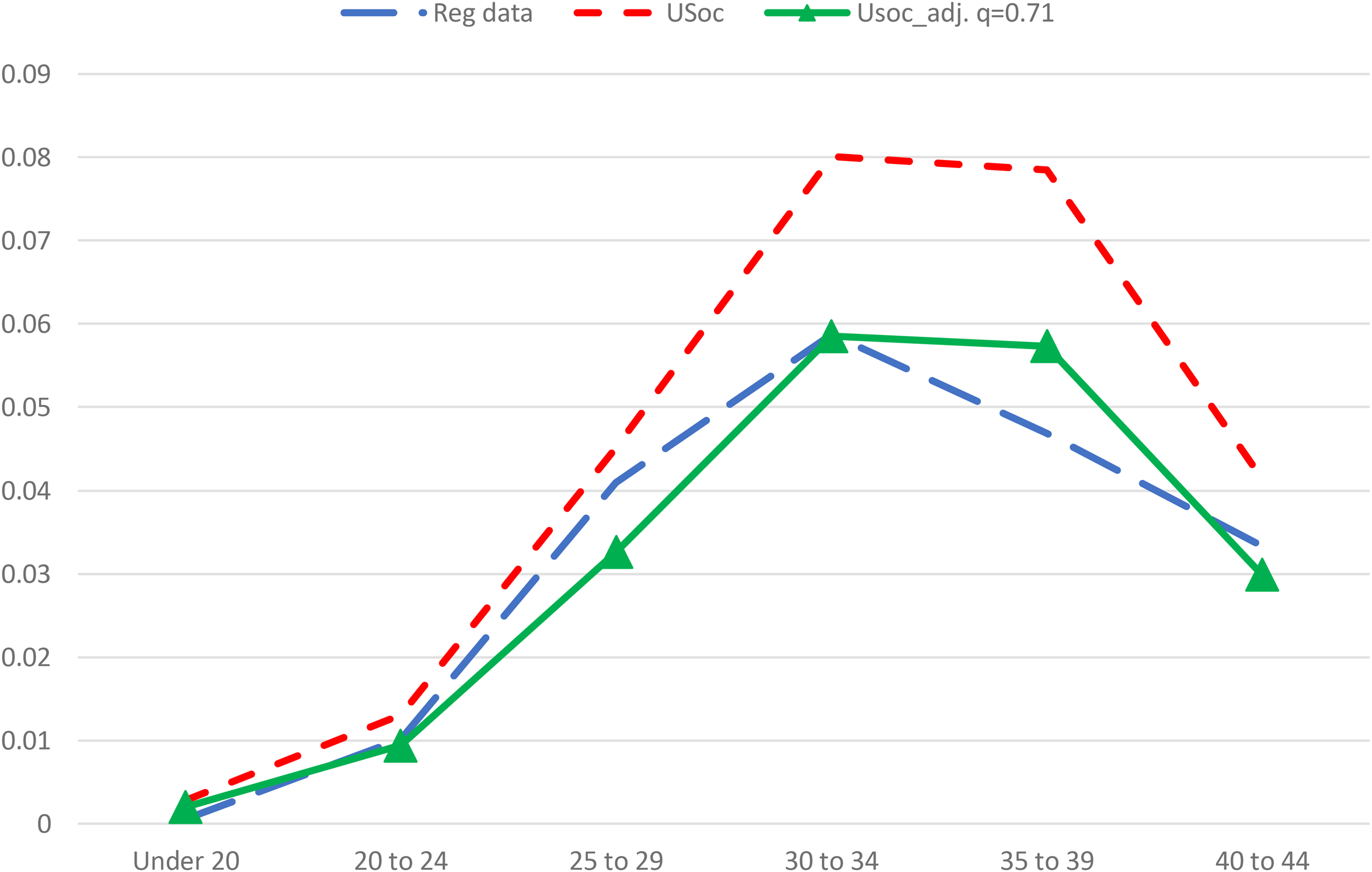
Figure 7 shows the comparison between men's age-specific average marriage rates for 2010–13 based on registration data and estimates from Understanding Society using waves 1–3. ¹¹ The first reason for non-ignorable attrition leads to understatement of marriage rates in the survey data, but the second leads to overstatement of marriage rates in the survey data. Figure 7 suggests the second reason dominates. A similar but smaller difference is evident for women (Appendix Figure A2, supplemental material)

Figure 7.

Marriage rates from registration data (average 2010–13) Understanding Society (waves 1–3) and adjusted Understanding Society rates (waves 1–3), men.

Estimation of $\hat{q}$ is analogous to the previous example using the six age group observations to estimate equation ( $3^{\mathrm{\prime }}$ ). The estimate of $\hat{q}$ is 0.71 (SE = 0.05) for men and 0.87 (SE = 0.03) for women. The survey marriage probability estimates adjusted using $\hat{q}$ are shown in Figure 7 (and Figure A2) as the lines with triangles.

The marriage example addresses a simple substantive question which cannot be addressed with registration data: are people in a cohabiting couple more likely to marry if they have children than if they do not? A logit model for marrying between waves t and t + 1 was estimated, in which there are two sets of regressors: a quadratic in age and three variables for a two-way interaction between having a partner and having their own child(ren) in the household at wave t. The estimation was performed separately by gender.

Among partnered women in the survey data, after reweighting $mean[{\widehat{CME}}_i(Z)|R_i=1]$ of having a child is −0.023 (SE = 0.009), and $mean[{\widehat{UME}}_i(Z)|R_i=1]$ is −0.022. ¹² Among men, these quantities are −0.024 (SE = 0.010), and −0.018, respectively. Because having a child in the household also reduced panel retention, using $\hat{q}$ to adjust the conditional estimate may “over-adjust”; that is, it is possible that $mean[{\widehat{CME}}_i(Z)|R_i=1]$ is the superior estimator (closer to the true value than $mean[{\widehat{UME}}_i(Z)|R_i=1])$ . ¹³ This is not a large concern here because the differences between the $mean[{\widehat{CME}}_i(Z)|R_i=1]$ and the $mean[{\widehat{UME}}_i|R_i=1]$ are well within one standard error of $mean[{\widehat{CME}}_i(Z)|R_i=1]$ .

Conclusions

Empirical analysis of variation in demographic events within the population is facilitated by using longitudinal survey data, but there is wave-on-wave dropout. When attrition is related to the event, such as residential mobility, it precludes consistent estimation of the impacts of covariates on the event, on event probabilities and on statistics based on these probabilities in the absence of additional, unverifiable assumptions. The paper introduced an adjustment procedure based on Bayes Theorem that uses population information external to the survey sample to convert estimates of event probabilities and marginal effects of covariates on them that are conditional on retention in the longitudinal data to unconditional estimates of these quantities. ¹⁴ It does not produce consistent estimates of the unconditional quantities, but (1) its estimate of the mean unconditional probability of the event is always closer to the true value than the conditional estimate, with the adjustment factor providing a measure of how close the mean unconditional probability of the event is to its conditional estimate; and (2) estimation of the impacts of covariates on panel retention provides information on whether the adjusted estimates of the marginal effects of covariates are closer to the true unconditional values than the corresponding conditional estimates. The process of obtaining the adjusted estimator and the estimation of the propensity score equation reveals valuable information about the survey data relative to corresponding population data and whether attrition is ignorable or not, and reporting both estimates is recommended.

The adjustment method was applied to estimate the variation in residential mobility and marriage rates within the population in relation to covariates. The two sources of external population data are census and marriage registration statistics, respectively. In each case, the survey data was the large UK household panel survey called Understanding Society. In the residential mobility analysis, the conditional estimates understate the unconditional mean event probability substantially and the relationship between panel retention and the covariates is such that the adjusted estimates of the marginal effects are larger than the conditional estimate and very likely to be superior to the conditional ones. In the marriage analysis, the opposite is the case: the conditional mean probability overstates the unconditional one and the conditional estimate of the marginal effects is superior to the adjusted estimate, although similar.