The Design and Optimality of Survey Counts: A Unified Framework Via the Fisher Information Maximizer

Abstract

Grouped and right-censored (GRC) counts have been used in a wide range of attitudinal and behavioural surveys yet they cannot be readily analyzed or assessed by conventional statistical models. This study develops a unified regression framework for the design and optimality of GRC counts in surveys. To process infinitely many grouping schemes for the optimum design, we propose a new two-stage algorithm, the Fisher Information Maximizer (FIM), which utilizes estimates from generalized linear models to find a global optimal grouping scheme among all possible $N$ -group schemes. After we define, decompose, and calculate different types of regressor-specific design errors, our analyses from both simulation and empirical examples suggest that: 1) the optimum design of GRC counts is able to reduce the grouping error to zero, 2) the performance of modified Poisson estimators using GRC counts can be comparable to that of Poisson regression, and 3) the optimum design is usually able to achieve the same estimation efficiency with a smaller sample size.

Introduction

Grouped and right-censored (GRC) counts in survey research refer to response categories of discrete-value survey questions consisting of both grouped (e.g., “3–5 times” rather than precise counts of “3 times”, “4 times”, or “5 times”) and right-censored counts (e.g., an open-ended category as “6 or more times”) (Coughlin 1990; Fu et al. 2020; Guo et al. 2020; Schaeffer and Dykema 2020, 2011; Willis 2004). The advantage of GRC counts is that they do not require exact enumerations of behavioural frequencies and thus reduce cognitive burdens in data collection. Especially when respondents seek to adopt a series of answering strategies to alleviate their cognitive burdens and provide good enough answers (Schaeffer and Dykema 2011; Gehlbach and Barge 2012; Conrad et al. 1998), the use of GRC counts is a convenient and inexpensive way of coping with cross-subject heterogeneity in understanding, interpreting, recalling, and estimating target events and behaviours. ¹ GRC counts have been recommended by survey methodologists over other alternative formats of response categories for studying event frequencies, especially when sensitive topics (e.g., drug use, juvenile delinquency, suicide attempts) or vulnerable populations (e.g., children, youth, the elderly) are being studied (Schaeffer and Dykema 2020; Schwarz et al. 1985; Toepoel et al. 2009). For example, two nationally-representative surveys on adolescent risky behaviours in America, the Monitoring the Future project and the Youth Risk Behavior Survey, use GRC counts to track temporal patterns of substance use and juvenile delinquency (Johnston et al. 2017; Kann et al. 2018). The National Longitudinal Study of Adolescent to Adult Health (Add Health), which is the largest longitudinal survey of adolescents in America, also relies on GRC counts to collect information on various health-related outcomes (Bahr and Hoffmann 2008; Conway et al. 2013).

Although GRC counts have been widely used in survey research (Ackard et al. 2002; Akers et al. 1989; Bachman et al. 1990; Baiden et al. 2019; Fu et al. 2013; Hagan et al. 2005; Kumar et al. 2008; Marsden 2003), their design and analysis create methodological challenges. Due to the lack of conventional tools to capture the data generating process of GRC counts, they are often treated as categories instead of counts, and accordingly analyzed by (ordinal/multinomial) logistic regression models instead of Poisson-based models (Connor et al. 2013; John et al. 2006). While some recent studies have attempted to implement regression models and derive asymptotic properties of estimators to analyze GRC counts (Fu et al. 2021; Guo et al. 2020; Wang 2022), the optimum survey design of GRC counts in a regression setting remains a critical yet challenging issue faced by survey methodologists and social scientists in general.

More specifically, the optimum survey design of GRC counts in a regression setting needs to take three key issues into account (Fu et al. 2020; Biemer 2010). First, to achieve the optimum design, a search algorithm should be designed to incorporate available information on regression covariates, process infinitely many grouping schemes for GRC counts, and identify an optimal grouping scheme that maximizes (a score function of) the Fisher information matrix of the population parameters to achieve maximum estimation efficiency. Second, for a specific (and usually suboptimal) scheme chosen by researchers, its difference from the identified optimal grouping scheme and the impact of such difference on statistical inference need to be assessed. Third, to establish optimality criteria for assessing grouping schemes, design errors associated with grouping schemes also need to be defined, decomposed, and calculated. By critically synthesizing and greatly extending a series of recent advances in the design and analysis of GRC counts (Davillas and Pudney 2020; Fu et al. 2020; Guo et al. 2020; Schaeffer and Dykema 2020), the current study addresses these three issues. While the optimum design of GRC counts is the primary focus of this study, it should be noted that the unified framework to be described here also solves a more general question of optimality and design of counts when they are either grouped, right-censored, or both, in surveys.

Methods

Generalized Linear Models for Grouped and Right-Censored Counts

To characterize the data-generating distribution of GRC counts, we let $N\ge 2$ denote the total number of GRC response categories used in a survey question, and divide all non-negative integers into these $N$ groups. The $i$ ’th group ( $1\le i\le N$ ) consists of one or a successive sequence of integer(s),

$$\begin{array}{r}{\mathrm{Group}}_i=\{k\in \mathbb{N}:l_i\le k<l_{i+1}\},\end{array}$$

where $\mathbb{N}=\{0,1,2,\dots \}$ is the totality of all the non-negative integers, and $0=l_1<l_2<\cdots <l_{N+1}=\mathrm{\infty }$ are used to define boundaries separating these $N$ groups of an $N$ -group scheme.

We first illustrate how generalized linear models (GLMs) are used to analyze GRC counts. The choice of GLMs permits a more flexible parameterization of GRC counts, such as a zero-inflated model, a negative binomial model, a hurdle model, or a mixture of these models (Hilbe 2011; Land et al. 1996). We begin with the following GLM model, Poisson regression, which is well studied and widely used to model count data (Agresti 2003; Lawless 1987; Rhodes et al. 1996). Let $Y$ be a random variable that has a Poisson distribution $\mathrm{Pois}(\lambda )$ with mean $\lambda >0$ , namely, $\mathrm{Prob}(Y=k)=e^{-\lambda }{\lambda }^k/k!$ , for $k$ in $\mathbb{N}$ . In Poisson regression, the expected frequency $\lambda$ is specified by a linear combination of regressors $\mathit{X}=(X_0,\dots ,X_d{)}^T\in {\mathbb{R}}^{d+1}$ through a link function $\lambda =g_{\lambda }^{-1}({\mathit{\beta }}^{*T}\mathit{X})$ , where ${\mathit{\beta }}^{*}=({\beta }_0^{*},\dots ,{\beta }_d^{*}{)}^T\in \mathbb{R}$ is the vector of unknown coefficients.

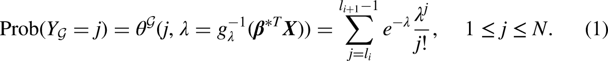
Instead of using exact enumeration in the original Poisson model, counts are now measured in a grouped and right-censored form given by $\mathcal{G}$ . Here, $\mathcal{G}=\{l_i{\}}_{i=1}^{N+1}$ refers to a GRC grouping scheme and $Y_{\mathcal{G}}$ is a random variable obtained by categorizing $Y$ with respect to $\mathcal{G}$ . Specifically, $Y_{\mathcal{G}}=i$ if and only if $Y$ is in the $i$ ’th group. So $Y_{\mathcal{G}}$ has a categorical distribution on $\{1,\dots ,N\}$ , with

$$\mathrm{Prob}(Y_{\mathcal{G}}=j)={\theta }^{\mathcal{G}}(j,\lambda =g_{\lambda }^{-1}({\mathit{\beta }}^{*T}\mathit{X}))=\sum _{j=l_i}^{l_{i+1}-1}{e}^{-\lambda }\frac{{\lambda }^j}{j!},1\le j\le N.$$

(1)

Based on (1), the modified log-likelihood function for a sample $\{({\mathit{X}}^i,Y_{\mathcal{G}}^i){\}}_{i=1}^n$ is

$${\ell }_n^{\mathcal{G}}(\mathit{\beta })=\sum _{i=1}^n\log {\theta }^{\mathcal{G}}(Y_{\mathcal{G}}^i,g_{\lambda }^{-1}({\mathit{\beta }}^T{\mathit{X}}^i)).$$

(2)

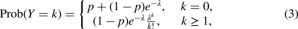
The Poisson distribution requires that the variance be the same as the mean. However, this equi-dispersion assumption is often violated due to the existence of excessive zeros (Fu et al. 2013; Tucker et al. 2021). The zero-inflated Poisson (ZIP) distribution incorporates a binomial process to take into account excessive zeros (Hall 2000; Lambert 1992; Land et al. 1996). Take binge drinking, for example: the ZIP distribution considers two potential sources of zeros. Those who are exposed to the risk of binge drinking but do not report any episode of binge drinking, and those who are not exposed to the risk of binge drinking due to various religious, health, or socio-relational factors (Jun et al. 2016; Luczak et al. 2002; Tucker et al. 2021). The probability mass function for the ZIP distribution is:

$$\mathrm{Prob}(Y=k)=\{\begin{array}{cc}p+(1-p)e^{-\lambda },& k=0,\\ (1-p)e^{-\lambda }\frac{{\lambda }^k}{k!},& k\ge 1,\end{array}$$

(3)

where $\lambda >0$ and $0<p<1$ . The ratio $(1-p)$ is the population’s proportion subject to $\mathrm{Pois}(\lambda )$ . Here $Y_{\mathcal{G}}$ also has a categorical distribution obtained by categorizing (3) according to $\mathcal{G}$ . The modified log-likelihood function is obtained by replacing the summand in (2) with $\log {\theta }^{\mathcal{G}}(Y_{\mathcal{G}}^i,g_{\lambda }^{-1}({\mathit{\beta }}^T{\mathit{X}}^i),g_p^{-1}({\mathit{\gamma }}^T{\mathit{U}}^i))$ , where ${\mathit{U}}^i$ represents the vector of regressors, the vector $\mathit{\gamma }$ denotes corresponding coefficients, and $g_p^{-1}({\mathit{\gamma }}^T{\mathit{U}}^i)$ is the generalized linear model for $p$ with the corresponding link function $g_p$ . The proof (available upon request) of existence, consistency, and asymptotic normality of these modified Poisson estimators readily follows (Fahrmeir and Kaufmann 1985; Fu et al. 2018; Serfling 1980).

Define and Decompose Design Errors of GRC Counts

To define and decompose errors in the optimum design of GRC counts, or more broadly, survey counts, we next investigate possible sources of errors. First, the total number of count response categories $N$ is restricted to be finite. As compared to the scenario of exact enumeration, the finite number of count response categories entails a loss of information in measurement and further leads to less efficient estimation. In other words, although $N$ corresponds to a measure of counts (of human behaviours) that are infinite in nature, the finiteness of $N$ originates from the total number of response categories fixed by survey investigators. The first design error is essentially a product of survey designs, rather than the finiteness of $N$ . We hereafter refer to this design error caused by the restriction in $N$ as the groups error. Second, with a finite $N$ , a suboptimal grouping scheme chosen by survey investigators from all possible $N$ -group schemes leads to less efficient estimation and produces the grouping error. Without the optimum design of survey counts, a grouping scheme specified by researchers is likely to be suboptimal. For example, the grouping error occurs when the most observed counts (e.g., 3 times and 4 times) are arbitrarily categorized in a wide group (e.g., 3 to 10 times). The sum of the groups and grouping errors gives the total error in the design of survey counts. The optimum design of survey counts, as we will show next, is able to reduce the grouping error to zero.

The asymptotic normality of modified Poisson estimators suggests that a suboptimal grouping scheme has less Fisher information. Based on the literature on optimum experimental designs (Atkinson et al. 2007; Goos et al. 2016), one may employ a score function (e.g., A-, D-, E-, or I-optimality) to compare Fisher information matrices of different grouping schemes and then decompose the total error into the groups and grouping errors. In particular, if $\mathbb{I}$ is a real strictly positive definite matrix, A-optimality maximizes $1/\mathrm{Trace}({\mathbb{I}}^{-1})$ , D-optimality maximizes the determinant of $\mathbb{I}$ , and E-optimality maximizes the minimum eigenvalue of $\mathbb{I}$ .

When $N=\mathrm{\infty }$ and each group only contains one integer, exact enumeration clearly provides the universal optimal grouping scheme that maximizes a score function. When $N$ is finite for survey counts, the search for a global optimal grouping scheme that eliminates the grouping error plays a key role in the optimum design. For a specific score function of Fisher information (matrix), the difference between a global optimal grouping scheme and the universal optimal scheme corresponds to the groups error, while the difference between the global optimal scheme and an actual scheme chosen by survey investigators corresponds to the grouping error.

The Optimum Design of GRC Counts: Fisher Information Maximizer

We develop and describe a two-stage search algorithm, the Fisher Information Maximizer (FIM), to achieve the optimum design of survey counts with generalized linear models (GLMs). The FIM specifically addresses two related methodological issues. First, how to process and assess infinitely many grouping schemes based on an optimality criterion. Second, how to utilize information provided by data so that the search algorithm is informed by generalized linear models (described in Section 2.1) of survey counts.

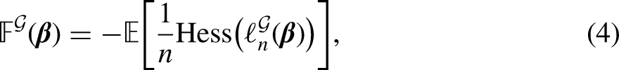
We focus on the modified Poisson model in (2) and the discussion can be readily extended to the ZIP case. The Fisher information matrix ${\mathbb{F}}^{\mathcal{G}}(\mathit{\beta })$ of Model (2) could be defined via the Hessian matrix $\mathrm{Hess}({\ell }_n^{\mathcal{G}}(\mathit{\beta }))$ of (2):

$${\mathbb{F}}^{\mathcal{G}}(\mathit{\beta })=-\mathbb{E}\left[\frac{1}{n}\mathrm{Hess}({\ell }_n^{\mathcal{G}}(\mathit{\beta }))\right],$$

(4)

where the mean is taken with respect to the sample $\{({\mathit{X}}^i,Y_{\mathcal{G}}^i){\}}_{i=1}^n$ . In particular, we have ${\mathbb{F}}^{\mathcal{G}}(\mathit{\beta })=-\mathbb{E}[\mathrm{Hess}({\ell }_1^{\mathcal{G}}(\mathit{\beta }))]$ . We omit the measure-theoretic discussion and assume that (4) is well defined and finite for all $\mathit{\beta }\in {\mathbb{R}}^{d+1}$ . Since we usually have no knowledge of the marginal distribution on the input space ${\mathbb{R}}^{d+1}$ , ${\mathbb{F}}^{\mathcal{G}}$ is replaced by a statistic

$$\begin{array}{r}{\mathbb{F}}_X^{\mathcal{G}}(\mathit{\beta }):=-\mathbb{E}[\frac{1}{n}\mathrm{Hess}({\ell }_n^{\mathcal{G}}(\mathit{\beta }))|{\left\{{\mathit{X}}^i\right\}}_{i=1}^n]=-\frac{1}{n}\sum _{i=1}^n\mathbb{E}[\mathrm{Hess}({\ell }_1^{\mathcal{G}}(\mathit{\beta }))\mid \mathit{X}={\mathit{X}}^i],\end{array}$$

where the conditional expectations are finite sums and easy to calculate.

Let $\mathcal{G}$ and ${\mathcal{G}}^{\prime }$ be two grouping schemes. We say that ${\mathcal{G}}^{\prime }$ is finer than $\mathcal{G}$ if $\mathcal{G}\subset {\mathcal{G}}^{\prime }$ . For example, the grouping scheme [never, 1–2 times, 3–5 times, 6–9 times, 10+ times] is finer than [never, 1–2 times, 3–9 times, 10+ times]. When $\mathcal{G}\subset {\mathcal{G}}^{\prime }$ , one has ${\mathbb{F}}_X^{\mathcal{G}}(\mathit{\beta })⪯{\mathbb{F}}_X^{{\mathcal{G}}^{\prime }}(\mathit{\beta })$ and ${\mathbb{F}}^{\mathcal{G}}(\mathit{\beta })⪯{\mathbb{F}}^{{\mathcal{G}}^{\prime }}(\mathit{\beta })$ for Poisson-based models (proof available upon request). Here, for two symmetric matrices $A$ and $B$ , one writes $A⪰B$ or $B⪯A$ , if $A-B$ is positive semi-definite. This agrees with the intuition that, for both Poisson and ZIP models, a finer grouping scheme always leads to a more efficient estimation. This monotonicity condition has two implications. First, the estimation based on schemes without grouping or right censoring achieves maximum efficiency. Second, with the restriction of no more than $N$ groups in any grouping scheme, a global optimal grouping scheme can always be found among the schemes with exactly $N$ groups.

Drawing on ideas from optimum experimental design (Atkinson et al. 2007; Goos et al. 2016), we develop the FIM to find a global optimal design among all the $N$ -group schemes with generalized linear models. Let $\omega$ be a function defined on the space of strictly positive definite matrices such that

$$\omega (A)\ge \omega (B),\text{whenever }A⪰B.$$

(5)

The requirement in (5) makes the scores $\omega ({\mathbb{F}}^{\mathcal{G}})$ and $\omega ({\mathbb{F}}_X^{\mathcal{G}})$ monotonic functions of the grouping schemes, where $\omega$ may take the form of the A-, D-, E-, or I-optimality scores (Atkinson et al. 2007).

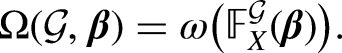
For any grouping scheme $\mathcal{G}$ and a coefficient vector $\mathit{\beta }$ , we define $\mathrm{\Omega }$ as follows to apply the search algorithm:

$$\begin{array}{r}\mathrm{\Omega }(\mathcal{G},\mathit{\beta })=\omega ({\mathbb{F}}_X^{\mathcal{G}}(\mathit{\beta })).\end{array}$$

We use $M$ , ${\mathcal{F}}_N$ , and ${\mathcal{F}}_{N,M}$ to denote a sufficiently large integer, the family of all $N$ -group schemes, and the subset of ${\mathcal{F}}_N$ with $M$ contained in the last group, respectively. For positive semi-definite matrices $A$ , $B$ , and $C$ , $\omega (A)\ge \omega (B)$ does not necessarily lead to $\omega (A+C)\ge \omega (B+C)$ so that the dynamic programming approach (Bai and Perron 2003) cannot be applied. The maximization of $\mathrm{\Omega }(\cdot ,\hat{\mathit{\beta }})$ over ${\mathcal{F}}_{N,M}$ (where $\hat{\mathit{\beta }}$ is an estimate of ${\mathit{\beta }}^{*}$ obtained, for example, from a pilot study) is then thwarted by two problems: the computation of ${\mathbb{F}}_X^{\mathcal{G}}(\hat{\mathit{\beta }})$ is time consuming, and one has a large set of grouping schemes to assess.

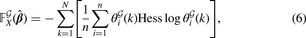
To solve these problems, the synthesis stage of the FIM computes the “building blocks” of ${\mathbb{F}}_X^{\mathcal{G}}(\hat{\mathit{\beta }})$ , and then synthesizes the Fisher information matrices by adding up the corresponding blocks. More specifically, for $\mathcal{G}=\{l_i{\}}_{i=1}^{N+1}$ , we have

$${\mathbb{F}}_X^{\mathcal{G}}(\hat{\mathit{\beta }})=-\sum _{k=1}^N[\frac{1}{n}\sum _{i=1}^n{\theta }_i^{\mathcal{G}}(k)\mathrm{Hess}\log {\theta }_i^{\mathcal{G}}(k)],$$

(6)

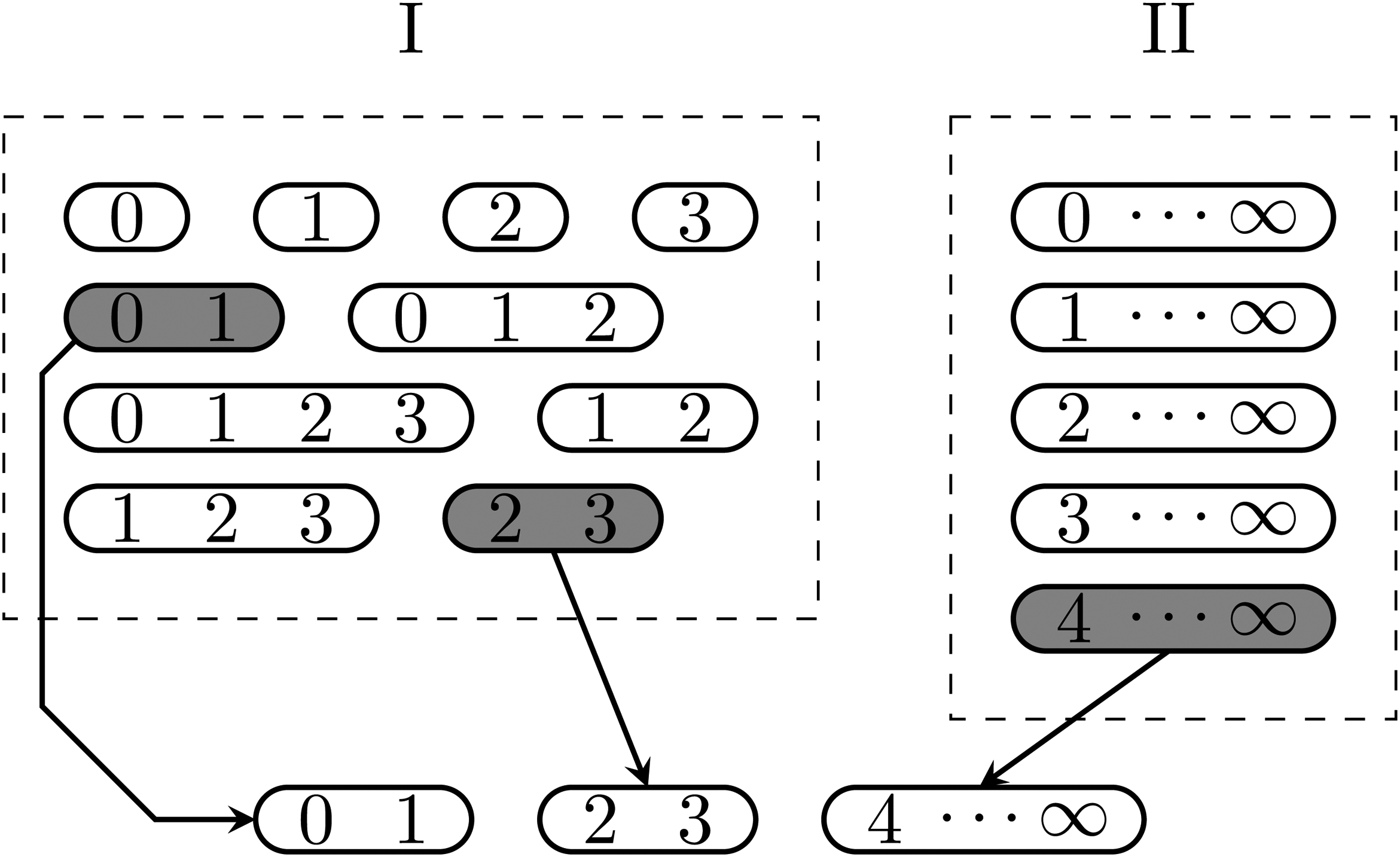
where ${\theta }_i^{\mathcal{G}}(k)=\sum _{j=l_k}^{l_{k+1}-1}{e}^{-{\lambda }_i}{\lambda }_i^j/j!$ , ${\lambda }_i=g_{\lambda }^{-1}({\hat{\mathit{\beta }}}^T{\mathit{X}}^i)$ , and the Hessian is taken with respect to the vector $\mathit{\beta }$ at $\mathit{\beta }=\hat{\mathit{\beta }}$ . In (6), the expression in the square bracket can be calculated before the choice of a grouping scheme $\mathcal{G}$ because the calculation only needs to specify the pair $(l_k,l_{k+1})$ defining the boundaries of a group to be included in $\mathcal{G}$ . The FIM’s synthesis stage is illustrated with the example $\mathcal{G}=\{0,2,4,\mathrm{\infty }\}$ in Figure 1. Instead of assessing infinitely many grouping schemes, the FIM considers two finite sets of groups for building a grouping scheme through the introduction of $M$ : the first set (dashed box I) consists of all possible groups not containing any integer $\ge M$ , while the second set (dashed box II) consists of all possible groups containing all the integers $\ge M$ . A building block (i.e., the Fisher information matrix of a group in the dashed boxes) is computed, stored, and later retrieved to synthesize ${\mathbb{F}}_X^{\mathcal{G}}$ of a specific grouping scheme.

Figure 1.

An illustration of the synthesis stage of the FIM: synthesizing ${\mathbb{F}}_X^{\mathcal{G}}$ with $\mathcal{G}=\{0,2,4,\mathrm{\infty }\}$ .

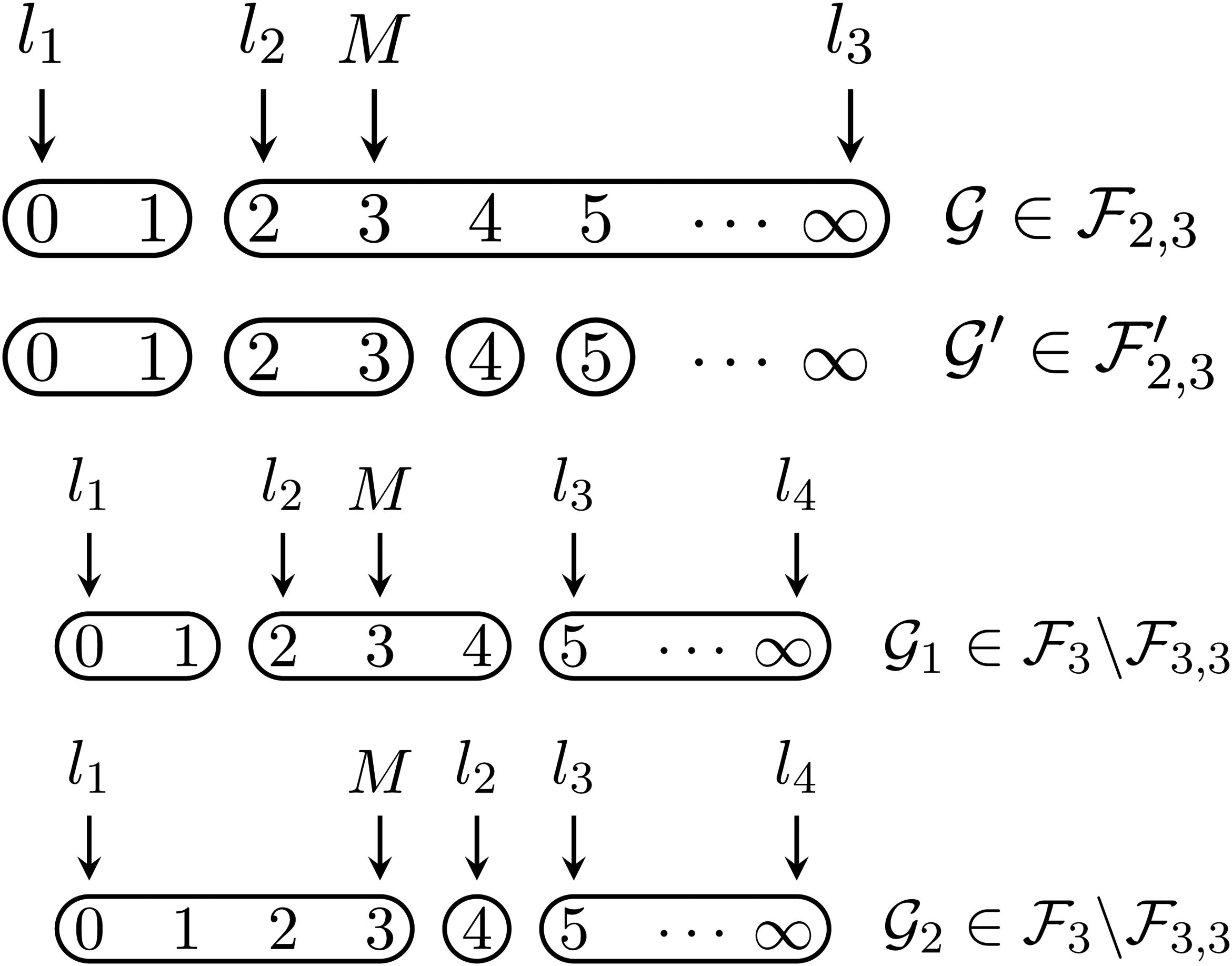
We use ${\mathcal{G}}_M$ to denote the maximizer of $\mathrm{\Omega }(\cdot ,\hat{\mathit{\beta }})$ on ${\mathcal{F}}_{N,M}$ . In the next validation stage of the FIM, the FIM proceeds differently depending on whether ${\mathcal{G}}_M$ is validated as the maximizer of $\mathrm{\Omega }(\cdot ,\hat{\mathit{\beta }})$ on ${\mathcal{F}}_N$ . We define ${\mathcal{F}}_{N-1,M}^{\prime }$ as the totality of all the schemes ${\mathcal{G}}^{\prime }$ , which are obtained from some $\mathcal{G}\in {\mathcal{F}}_{N-1,M}$ by dividing every integer larger than $M$ into a separate group. For every scheme $\mathcal{G}$ in ${\mathcal{F}}_N\mathrm{\setminus }{\mathcal{F}}_{N,M}$ , there is some ${\mathcal{G}}^{\prime }$ in ${\mathcal{F}}_{N-1,M}^{\prime }$ that is finer than $\mathcal{G}$ ; the size of ${\mathcal{F}}_{N-1,M}^{\prime }$ cannot be larger than that of ${\mathcal{F}}_{N-1,M}$ . We then compare $max\{\mathrm{\Omega }(\mathcal{G},\hat{\mathit{\beta }}):\mathcal{G}\in {\mathcal{F}}_{N-1,M}^{\prime }\}$ with $\mathrm{\Omega }({\mathcal{G}}_M,\hat{\mathit{\beta }})$ . If the latter is not smaller, ${\mathcal{G}}_M$ is guaranteed to be the maximizer of $\mathrm{\Omega }(\cdot ,\hat{\mathit{\beta }})$ on ${\mathcal{F}}_N$ . Otherwise one may choose a larger $M$ and start over. The specified integer $M$ controls the sizes of ${\mathcal{F}}_{N,M}$ and ${\mathcal{F}}_{N-1,M}^{\prime }$ so that a larger $M$ is associated with a longer search time. Yet, $M$ should be large enough to pass the aforementioned validation criterion, namely, $\mathrm{\Omega }({\mathcal{G}}_M,\hat{\mathit{\beta }})$ is not smaller than $max\{\mathrm{\Omega }(\mathcal{G},\hat{\mathit{\beta }}):\mathcal{G}\in {\mathcal{F}}_{N-1,M}^{\prime }\}$ . The FIM’s validation stage is illustrated with the example $M=N=3$ in Figure 2, where ${\mathcal{G}}^{\prime }$ is clearly finer than both ${\mathcal{G}}_1$ and ${\mathcal{G}}_2$ in ${\mathcal{F}}_3\mathrm{\setminus }{\mathcal{F}}_{3,3}$ .

Figure 2.

An illustration of the validation stage of the FIM: validating maximizers with $M=N=3$ .

Calculate Design Errors and Assess Grouping Schemes

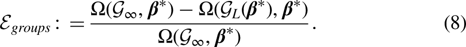
We now use ${\mathcal{G}}_{\mathsf{C}}$ to denote the current $N$ -group scheme chosen by survey investigators. Given a coefficient vector $\mathit{\beta }$ and a data matrix $\mathit{X}$ , we use ${\mathcal{G}}_{\mathsf{L}}(\mathit{\beta })$ to denote the global maximizer of $\mathrm{\Omega }(\cdot ,\mathit{\beta })$ among all possible $N$ -group schemes. In other words, ${\mathcal{G}}_{\mathsf{L}}(\mathit{\beta })$ is the maximizer of $\mathrm{\Omega }(\cdot ,\mathit{\beta })$ on ${\mathcal{F}}_N$ , which can be obtained by the FIM. We next define ${\mathcal{G}}_{\mathrm{\infty }}$ as the grouping scheme that each group only contains one non-negative integer, which corresponds to the scenario of exact enumeration of counts in conventional Poisson regression. As we discussed above, ${\mathcal{G}}_{\mathrm{\infty }}$ is the universal maximizer of $\mathrm{\Omega }$ . The groups and grouping errors, both of which are non-negative by definition, are given below:

$${\mathcal{E}}_{\mathsf{g}\mathsf{r}\mathsf{o}\mathsf{u}\mathsf{p}\mathsf{i}\mathsf{n}\mathsf{g}}={\mathcal{E}}_{\mathsf{g}\mathsf{r}\mathsf{o}\mathsf{u}\mathsf{p}\mathsf{i}\mathsf{n}\mathsf{g}}({\mathcal{G}}_{\mathsf{C}},{\mathit{\beta }}^{*}):=\frac{\mathrm{\Omega }({\mathcal{G}}_{\mathsf{L}}({\mathit{\beta }}^{*}),{\mathit{\beta }}^{*})-\mathrm{\Omega }({\mathcal{G}}_{\mathsf{C}},{\mathit{\beta }}^{*})}{\mathrm{\Omega }({\mathcal{G}}_{\mathrm{\infty }},{\mathit{\beta }}^{*})},$$

(7)

$${\mathcal{E}}_{\mathsf{g}\mathsf{r}\mathsf{o}\mathsf{u}\mathsf{p}\mathsf{s}}:=\frac{\mathrm{\Omega }({\mathcal{G}}_{\mathrm{\infty }},{\mathit{\beta }}^{*})-\mathrm{\Omega }({\mathcal{G}}_{\mathsf{L}}({\mathit{\beta }}^{*}),{\mathit{\beta }}^{*})}{\mathrm{\Omega }({\mathcal{G}}_{\mathrm{\infty }},{\mathit{\beta }}^{*})}.$$

(8)

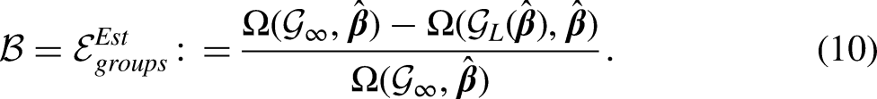
For empirical applications, the true coefficient vector ${\mathit{\beta }}^{*}$ is unknown, so neither of the errors is computable. We define ${\mathcal{E}}_{\mathsf{g}\mathsf{r}\mathsf{o}\mathsf{u}\mathsf{p}\mathsf{i}\mathsf{n}\mathsf{g}}^{\mathsf{E}\mathsf{s}\mathsf{t}}$ and ${\mathcal{E}}_{\mathsf{g}\mathsf{r}\mathsf{o}\mathsf{u}\mathsf{p}\mathsf{s}}^{\mathsf{E}\mathsf{s}\mathsf{t}}$ in the same way as in (7) and (8), respectively, substitute ${\mathit{\beta }}^{*}$ with its estimate $\hat{\mathit{\beta }}$ from generalized linear models, and have:

$$\mathcal{A}={\mathcal{E}}_{\mathsf{g}\mathsf{r}\mathsf{o}\mathsf{u}\mathsf{p}\mathsf{i}\mathsf{n}\mathsf{g}}^{\mathsf{E}\mathsf{s}\mathsf{t}}={\mathcal{E}}_{\mathsf{g}\mathsf{r}\mathsf{o}\mathsf{u}\mathsf{p}\mathsf{i}\mathsf{n}\mathsf{g}}^{\mathsf{E}\mathsf{s}\mathsf{t}}({\mathcal{G}}_{\mathsf{C}},\hat{\mathit{\beta }}):=\frac{\mathrm{\Omega }({\mathcal{G}}_{\mathsf{L}}(\hat{\mathit{\beta }}),\hat{\mathit{\beta }})-\mathrm{\Omega }({\mathcal{G}}_{\mathsf{C}},\hat{\mathit{\beta }})}{\mathrm{\Omega }({\mathcal{G}}_{\mathrm{\infty }},\hat{\mathit{\beta }})},$$

(9)

$$\mathcal{B}={\mathcal{E}}_{\mathsf{g}\mathsf{r}\mathsf{o}\mathsf{u}\mathsf{p}\mathsf{s}}^{\mathsf{E}\mathsf{s}\mathsf{t}}:=\frac{\mathrm{\Omega }({\mathcal{G}}_{\mathrm{\infty }},\hat{\mathit{\beta }})-\mathrm{\Omega }({\mathcal{G}}_{\mathsf{L}}(\hat{\mathit{\beta }}),\hat{\mathit{\beta }})}{\mathrm{\Omega }({\mathcal{G}}_{\mathrm{\infty }},\hat{\mathit{\beta }})}.$$

(10)

In general, to compute and assess design errors, we treat these estimates inferred using modified Poisson models as prior information, identify a global optimal scheme that maximizes the score function via the FIM, and then use the diagonal elements of the inverse Fisher information matrix ² to calculate regressor-specific design errors.

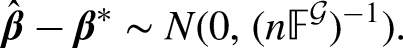
To take into account the design effect and calculate the effective sample size, we note that the estimator $\hat{\mathit{\beta }}$ with grouping scheme $\mathcal{G}$ and sample size $n$ has approximately a normal distribution centred on the true coefficient vector ${\mathit{\beta }}^{*}$ ,

$$\hat{\mathit{\beta }}-{\mathit{\beta }}^{*}\sim N(0,(n{\mathbb{F}}^{\mathcal{G}}{)}^{-1}).$$

Here, the covariance matrix $(n{\mathbb{F}}^{\mathcal{G}}{)}^{-1}$ considers the influence of the sampling error: a “smaller” covariance matrix indicates a smaller error, whereas the “larger” Fisher information matrix provides more efficient parameter estimation.

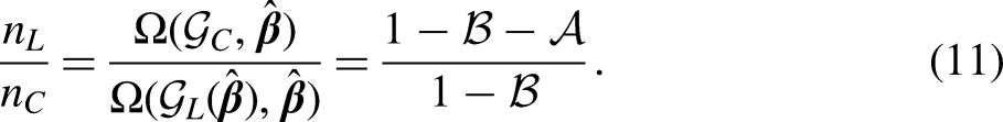
An optimal grouping scheme can usually achieve the same estimation efficiency with a smaller sample size. The FIM also allows us to assess relative estimation efficiencies based on different grouping schemes. We let $n_1$ and $n_2$ be the corresponding sample sizes of two different grouping schemes ${\mathcal{G}}_1$ and ${\mathcal{G}}_2$ , respectively, and use the following equation:

$$\omega (n_1{\mathbb{F}}_X^{{\mathcal{G}}_1}(\hat{\mathit{\beta }}))=\omega (n_2{\mathbb{F}}_X^{{\mathcal{G}}_2}(\hat{\mathit{\beta }})),$$

to calculate the ratio $n_1/n_2$ , which suggests the relative efficiency. The estimation efficiency based on ${\mathcal{G}}_2$ is more efficient relative to that based on ${\mathcal{G}}_1$ if $n_1/n_2$ is larger than 1. Here, we adopt the $A$ -optimality score function to make a comparison between Fisher information matrices:

$$\omega (\mathbb{F})=1/\mathsf{T}\mathsf{r}\mathsf{a}\mathsf{c}\mathsf{e}({\mathbb{F}}^{-1}).$$

For any number $c>0$ , we have $\omega (c\mathbb{F})=c\omega (\mathbb{F})$ .

We use $n_{\mathsf{L}}$ and $n_{\mathsf{C}}$ to denote sample sizes associated with the grouping scheme ${\mathcal{G}}_{\mathsf{L}}$ and ${\mathcal{G}}_{\mathsf{C}}$ , respectively. Based on calculated design errors in (9) and (10), we have

$$\frac{n_{\mathsf{L}}}{n_{\mathsf{C}}}=\frac{\mathrm{\Omega }({\mathcal{G}}_{\mathsf{C}},\hat{\mathit{\beta }})}{\mathrm{\Omega }({\mathcal{G}}_{\mathsf{L}}(\hat{\mathit{\beta }}),\hat{\mathit{\beta }})}=\frac{1-\mathcal{B}-\mathcal{A}}{1-\mathcal{B}}.$$

(11)

Using generalized linear models, the calculation of both design errors and the assessment of grouping schemes is regressor-specific.

Simulation and Empirical Results

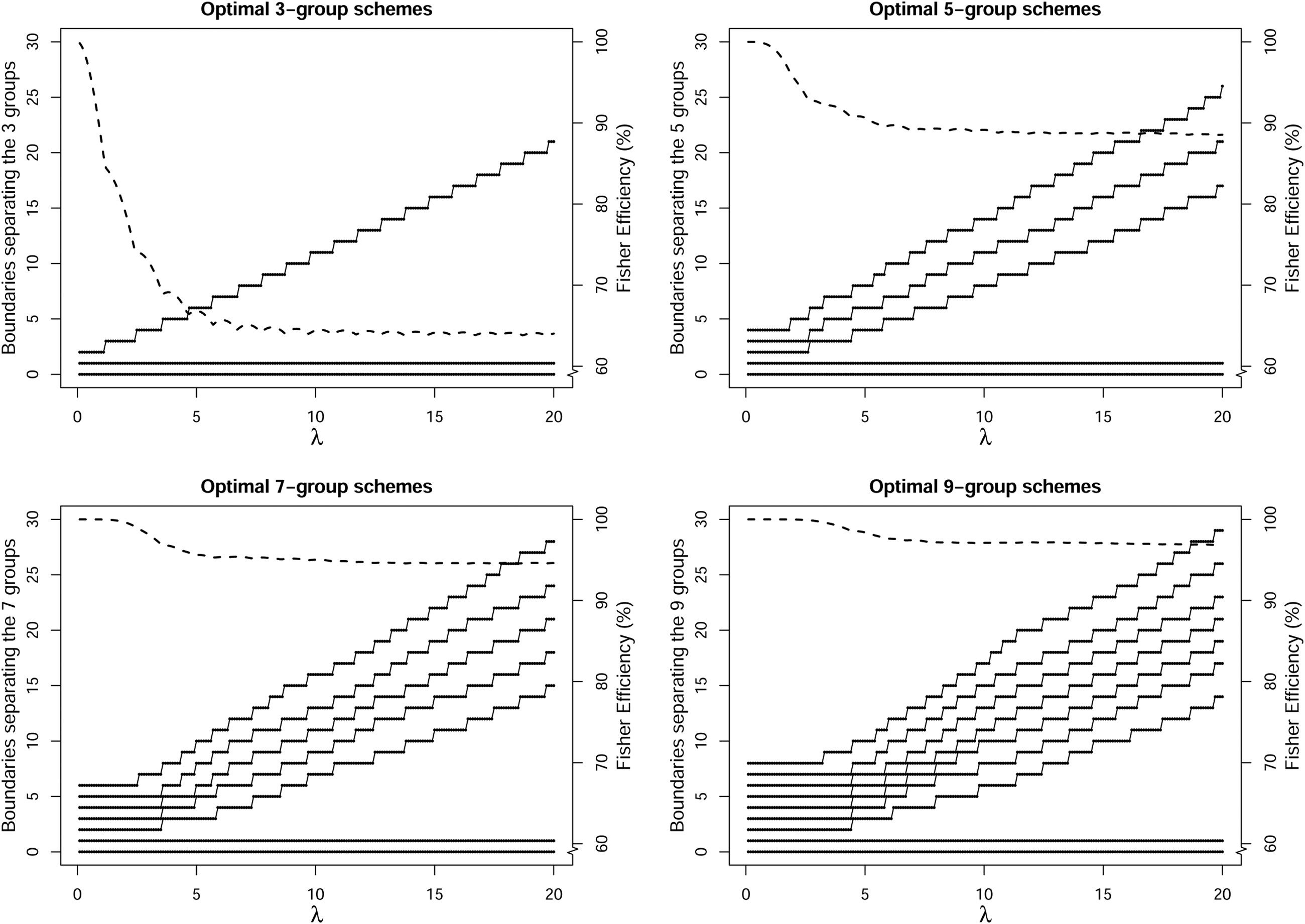
Based on different combinations of $\lambda$ (200 values evenly spaced from $0.1$ to $20$ ) and $N$ (3, 5, 7, and 9), we apply the FIM to empty models (models without covariates), identify an optimal grouping scheme with respect to each combination, and plot the boundaries of these optimal grouping schemes in Figure 3. For a specific $\lambda$ , the boundaries separating the $N$ groups of an optimal $N$ -group scheme are plotted in dots, and then linked by solid lines across different values of $\lambda$ . With a specific combination of $\lambda$ and $N$ , a point in the dashed line denotes the efficiency of a modified Poisson estimator with an optimal $N$ -group scheme relative to the conventional Poisson-regression estimator. The denominator of the relative efficiency is Fisher information of the conventional Poisson-regression estimator $1/\lambda$ . Following a general practice in survey research (Coughlin 1990; Johnston et al. 2017; Kann et al. 2018), zero is designed to be contained in a separate group.

Figure 3.

Boundaries of optimal grouping schemes (solid lines) and relative efficiencies of modified Poisson estimators (the axis of dashed lines starts from 60%) with combinations of $\lambda$ (evenly spaced from $0.1$ to $20$ ) and $N$ (3, 5, 7, and 9).

Except for the first group (containing zeros), integers separating groups demonstrate an increase with a larger $\lambda$ in all scenarios. When the total number of groups is small ( $N=3$ ), the relative efficiency decreases substantially (to around 60%) with a larger $\lambda$ but the decrease levels off around $\lambda =5$ . While a similar pattern holds for the other three scenarios (i.e., $N$ is 5, 7, and 9), it appears that such loss in the relative efficiency is greatly attenuated with a larger $N$ . As $\lambda$ approaches 20, the relative efficiency is still around 95% and 97% with $N=7$ and $N=9$ , respectively. These results suggest that, with a reasonably large $N$ and the optimal design of survey counts, the performance of modified Poisson estimators with grouped and/or right-censored counts is comparable to that of the conventional Poisson-regression estimator.

The second simulation study uses generalized linear models with covariates to investigate the finite-sample performance of different types of regressor-specific design errors. Based on the logarithm link function $g_{\lambda }(t)=\log t$ , we have the Poisson parameter $\lambda =g_{\lambda }^{-1}({\beta }_0+{\beta }_1{x}_1+{\beta }_2{x}_2)$ and set ${\beta }_0=-1$ , ${\beta }_1=1$ , and ${\beta }_2=2$ . Besides the logarithm link function, the ZIP case also uses the logit link $g_p(t)=\log \frac{t}{1-t}$ to consider the binomial parameter $p=g_p^{-1}({\gamma }_0+{\gamma }_1{u}_1)$ , where we set ${\gamma }_0=1$ and ${\gamma }_1=-1$ . The initial values of all the parameters are set to zero for maximum likelihood estimation and design errors are calculated based on 1000 replications with different sample sizes ( $n=400$ , $1200$ , $3600$ , and $10800$ ).

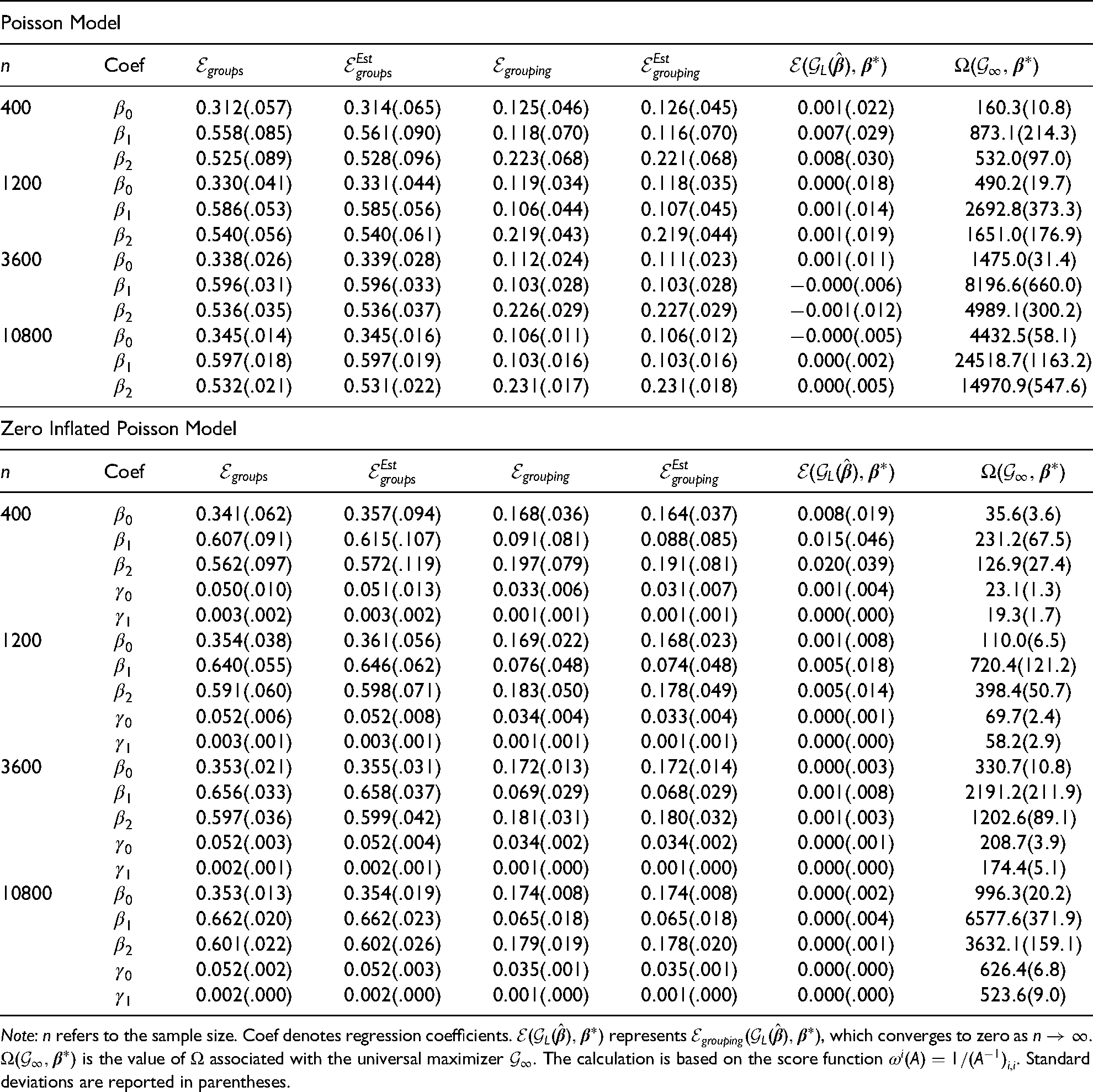
For each parameter estimated with a specific sample size $n$ , their corresponding design errors ${\mathcal{E}}_{\mathsf{g}\mathsf{r}\mathsf{o}\mathsf{u}\mathsf{p}\mathsf{s}}$ , ${\mathcal{E}}_{\mathsf{g}\mathsf{r}\mathsf{o}\mathsf{u}\mathsf{p}\mathsf{s}}^{\mathsf{E}\mathsf{s}\mathsf{t}}$ , ${\mathcal{E}}_{\mathsf{g}\mathsf{r}\mathsf{o}\mathsf{u}\mathsf{p}\mathsf{i}\mathsf{n}\mathsf{g}}$ and ${\mathcal{E}}_{\mathsf{g}\mathsf{r}\mathsf{o}\mathsf{u}\mathsf{p}\mathsf{i}\mathsf{n}\mathsf{g}}^{\mathsf{E}\mathsf{s}\mathsf{t}}$ (see Section 2.2) are reported. Because ${\mathcal{E}}_{\mathsf{g}\mathsf{r}\mathsf{o}\mathsf{u}\mathsf{p}\mathsf{s}}^{\mathsf{E}\mathsf{s}\mathsf{t}}$ and ${\mathcal{E}}_{\mathsf{g}\mathsf{r}\mathsf{o}\mathsf{u}\mathsf{p}\mathsf{i}\mathsf{n}\mathsf{g}}^{\mathsf{E}\mathsf{s}\mathsf{t}}$ are obtained by substituting ${\mathit{\beta }}^{*}$ with its estimate $\hat{\mathit{\beta }}$ , these two design errors are expected to be close to ${\mathcal{E}}_{\mathsf{g}\mathsf{r}\mathsf{o}\mathsf{u}\mathsf{p}\mathsf{s}}$ and ${\mathcal{E}}_{\mathsf{g}\mathsf{r}\mathsf{o}\mathsf{u}\mathsf{p}\mathsf{i}\mathsf{n}\mathsf{g}}$ , respectively, if the estimation is accurate. Likewise, by replacing ${\mathcal{G}}_{\mathsf{L}}({\mathit{\beta }}^{*})$ with ${\mathcal{G}}_{\mathsf{L}}(\hat{\mathit{\beta }})$ in (7), the grouping error ${\mathcal{E}}_{\mathsf{g}\mathsf{r}\mathsf{o}\mathsf{u}\mathsf{p}\mathsf{i}\mathsf{n}\mathsf{g}}({\mathcal{G}}_{\mathsf{L}}(\hat{\mathit{\beta }}),{\mathit{\beta }}^{*})$ is expected to converge to zero as $n\to \mathrm{\infty }$ . The value of $\mathrm{\Omega }$ associated with the universal maximizer ${\mathcal{G}}_{\mathrm{\infty }}$ , or $\mathrm{\Omega }({\mathcal{G}}_{\mathrm{\infty }},{\mathit{\beta }}^{*})$ , is also reported for readers’ reference. After 1000 replications, standard deviations of these estimated design errors are reported in parentheses. The grouping scheme of [never, 1–2 times, 3–5 times, 6–9 times, 10+ times] is used for all simulation scenarios.

Results from Table 1 clearly suggest the validity of the FIM. When actual parameters are replaced by sample estimates for both Poisson and ZIP cases, both ${\mathcal{E}}_{\mathsf{g}\mathsf{r}\mathsf{o}\mathsf{u}\mathsf{p}\mathsf{s}}^{\mathsf{E}\mathsf{s}\mathsf{t}}$ and ${\mathcal{E}}_{\mathsf{g}\mathsf{r}\mathsf{o}\mathsf{u}\mathsf{p}\mathsf{i}\mathsf{n}\mathsf{g}}^{\mathsf{E}\mathsf{s}\mathsf{t}}$ are very close to their counterparts ${\mathcal{E}}_{\mathsf{g}\mathsf{r}\mathsf{o}\mathsf{u}\mathsf{p}\mathsf{s}}$ and ${\mathcal{E}}_{\mathsf{g}\mathsf{r}\mathsf{o}\mathsf{u}\mathsf{p}\mathsf{i}\mathsf{n}\mathsf{g}}$ , respectively, even when the sample size is relatively small ( $n=400$ ). When the sample size becomes moderate or large, sample estimates are almost identical to actual parameters and their differences become negligible. Grouping errors ${\mathcal{E}}_{\mathsf{g}\mathsf{r}\mathsf{o}\mathsf{u}\mathsf{p}\mathsf{i}\mathsf{n}\mathsf{g}}({\mathcal{G}}_{\mathsf{L}}(\hat{\mathit{\beta }}),{\mathit{\beta }}^{*})$ are small and converge to zero as $n\to \mathrm{\infty }$ . As expected, $\mathrm{\Omega }({\mathcal{G}}_{\mathrm{\infty }},{\mathit{\beta }}^{*})$ increases with sample size. Design errors associated with the binomial part of ZIP models appear to be trivial as compared with those of Poisson models: the choice of grouping schemes has little impact on the estimation of the binomial parameters as long as the zero count (i.e., never) is contained in a separate group. In Table 1, groups errors appear to be higher than grouping errors for both Poisson and ZIP cases, but this conclusion is specific to the choice of simulation parameters and may not hold in other simulation or empirical scenarios.

Table 1.

Modified Poisson and ZIP models with GRC counts: regressor-specific design errors based on 1000 replications.

Poisson Model
$n$	Coef	${\mathcal{E}}_{\mathsf{g}\mathsf{r}\mathsf{o}\mathsf{u}\mathsf{p}\mathsf{s}}$	${\mathcal{E}}_{\mathsf{g}\mathsf{r}\mathsf{o}\mathsf{u}\mathsf{p}\mathsf{s}}^{\mathsf{E}\mathsf{s}\mathsf{t}}$	${\mathcal{E}}_{\mathsf{g}\mathsf{r}\mathsf{o}\mathsf{u}\mathsf{p}\mathsf{i}\mathsf{n}\mathsf{g}}$	${\mathcal{E}}_{\mathsf{g}\mathsf{r}\mathsf{o}\mathsf{u}\mathsf{p}\mathsf{i}\mathsf{n}\mathsf{g}}^{\mathsf{E}\mathsf{s}\mathsf{t}}$	$\mathcal{E}({\mathcal{G}}_{\mathsf{L}}(\hat{\mathit{\beta }}),{\mathit{\beta }}^{*})$	$\mathrm{\Omega }({\mathcal{G}}_{\mathrm{\infty }},{\mathit{\beta }}^{*})$
400	${\beta }_0$	$0.312(.057)$	$0.314(.065)$	$0.125(.046)$	$0.126(.045)$	$0.001(.022)$	$160.3(10.8)$
	${\beta }_1$	$0.558(.085)$	$0.561(.090)$	$0.118(.070)$	$0.116(.070)$	$0.007(.029)$	$873.1(214.3)$
	${\beta }_2$	$0.525(.089)$	$0.528(.096)$	$0.223(.068)$	$0.221(.068)$	$0.008(.030)$	$532.0(97.0)$
$1200$	${\beta }_0$	$0.330(.041)$	$0.331(.044)$	$0.119(.034)$	$0.118(.035)$	$0.000(.018)$	$490.2(19.7)$
	${\beta }_1$	$0.586(.053)$	$0.585(.056)$	$0.106(.044)$	$0.107(.045)$	$0.001(.014)$	$2692.8(373.3)$
	${\beta }_2$	$0.540(.056)$	$0.540(.061)$	$0.219(.043)$	$0.219(.044)$	$0.001(.019)$	$1651.0(176.9)$
3600	${\beta }_0$	$0.338(.026)$	$0.339(.028)$	$0.112(.024)$	$0.111(.023)$	$0.001(.011)$	$1475.0(31.4)$
	${\beta }_1$	$0.596(.031)$	$0.596(.033)$	$0.103(.028)$	$0.103(.028)$	$-0.000(.006)$	$8196.6(660.0)$
	${\beta }_2$	$0.536(.035)$	$0.536(.037)$	$0.226(.029)$	$0.227(.029)$	$-0.001(.012)$	$4989.1(300.2)$
10800	${\beta }_0$	$0.345(.014)$	$0.345(.016)$	$0.106(.011)$	$0.106(.012)$	$-0.000(.005)$	$4432.5(58.1)$
	${\beta }_1$	$0.597(.018)$	$0.597(.019)$	$0.103(.016)$	$0.103(.016)$	$0.000(.002)$	$24518.7(1163.2)$
	${\beta }_2$	$0.532(.021)$	$0.531(.022)$	$0.231(.017)$	$0.231(.018)$	$0.000(.005)$	$14970.9(547.6)$
Zero Inflated Poisson Model
$n$	Coef	${\mathcal{E}}_{\mathsf{g}\mathsf{r}\mathsf{o}\mathsf{u}\mathsf{p}\mathsf{s}}$	${\mathcal{E}}_{\mathsf{g}\mathsf{r}\mathsf{o}\mathsf{u}\mathsf{p}\mathsf{s}}^{\mathsf{E}\mathsf{s}\mathsf{t}}$	${\mathcal{E}}_{\mathsf{g}\mathsf{r}\mathsf{o}\mathsf{u}\mathsf{p}\mathsf{i}\mathsf{n}\mathsf{g}}$	${\mathcal{E}}_{\mathsf{g}\mathsf{r}\mathsf{o}\mathsf{u}\mathsf{p}\mathsf{i}\mathsf{n}\mathsf{g}}^{\mathsf{E}\mathsf{s}\mathsf{t}}$	$\mathcal{E}({\mathcal{G}}_{\mathsf{L}}(\hat{\mathit{\beta }}),{\mathit{\beta }}^{*})$	$\mathrm{\Omega }({\mathcal{G}}_{\mathrm{\infty }},{\mathit{\beta }}^{*})$
400	${\beta }_0$	$0.341(.062)$	$0.357(.094)$	$0.168(.036)$	$0.164(.037)$	$0.008(.019)$	$35.6(3.6)$
	${\beta }_1$	$0.607(.091)$	$0.615(.107)$	$0.091(.081)$	$0.088(.085)$	$0.015(.046)$	$231.2(67.5)$
	${\beta }_2$	$0.562(.097)$	$0.572(.119)$	$0.197(.079)$	$0.191(.081)$	$0.020(.039)$	$126.9(27.4)$
	${\gamma }_0$	$0.050(.010)$	$0.051(.013)$	$0.033(.006)$	$0.031(.007)$	$0.001(.004)$	$23.1(1.3)$
	${\gamma }_1$	$0.003(.002)$	$0.003(.002)$	$0.001(.001)$	$0.001(.001)$	$0.000(.000)$	$19.3(1.7)$
1200	${\beta }_0$	$0.354(.038)$	$0.361(.056)$	$0.169(.022)$	$0.168(.023)$	$0.001(.008)$	$110.0(6.5)$
	${\beta }_1$	$0.640(.055)$	$0.646(.062)$	$0.076(.048)$	$0.074(.048)$	$0.005(.018)$	$720.4(121.2)$
	${\beta }_2$	$0.591(.060)$	$0.598(.071)$	$0.183(.050)$	$0.178(.049)$	$0.005(.014)$	$398.4(50.7)$
	${\gamma }_0$	$0.052(.006)$	$0.052(.008)$	$0.034(.004)$	$0.033(.004)$	$0.000(.001)$	$69.7(2.4)$
	${\gamma }_1$	$0.003(.001)$	$0.003(.001)$	$0.001(.001)$	$0.001(.001)$	$0.000(.000)$	$58.2(2.9)$
3600	${\beta }_0$	$0.353(.021)$	$0.355(.031)$	$0.172(.013)$	$0.172(.014)$	$0.000(.003)$	$330.7(10.8)$
	${\beta }_1$	$0.656(.033)$	$0.658(.037)$	$0.069(.029)$	$0.068(.029)$	$0.001(.008)$	$2191.2(211.9)$
	${\beta }_2$	$0.597(.036)$	$0.599(.042)$	$0.181(.031)$	$0.180(.032)$	$0.001(.003)$	$1202.6(89.1)$
	${\gamma }_0$	$0.052(.003)$	$0.052(.004)$	$0.034(.002)$	$0.034(.002)$	$0.000(.001)$	$208.7(3.9)$
	${\gamma }_1$	$0.002(.001)$	$0.002(.001)$	$0.001(.000)$	$0.001(.000)$	$0.000(.000)$	$174.4(5.1)$
10800	${\beta }_0$	$0.353(.013)$	$0.354(.019)$	$0.174(.008)$	$0.174(.008)$	$0.000(.002)$	$996.3(20.2)$
	${\beta }_1$	$0.662(.020)$	$0.662(.023)$	$0.065(.018)$	$0.065(.018)$	$0.000(.004)$	$6577.6(371.9)$
	${\beta }_2$	$0.601(.022)$	$0.602(.026)$	$0.179(.019)$	$0.178(.020)$	$0.000(.001)$	$3632.1(159.1)$
	${\gamma }_0$	$0.052(.002)$	$0.052(.003)$	$0.035(.001)$	$0.035(.001)$	$0.000(.000)$	$626.4(6.8)$
	${\gamma }_1$	$0.002(.000)$	$0.002(.000)$	$0.001(.000)$	$0.001(.000)$	$0.000(.000)$	$523.6(9.0)$

Note: $n$ refers to the sample size. Coef denotes regression coefficients. $\mathcal{E}({\mathcal{G}}_{\mathsf{L}}(\hat{\mathit{\beta }}),{\mathit{\beta }}^{*})$ represents ${\mathcal{E}}_{\mathsf{g}\mathsf{r}\mathsf{o}\mathsf{u}\mathsf{p}\mathsf{i}\mathsf{n}\mathsf{g}}({\mathcal{G}}_{\mathsf{L}}(\hat{\mathit{\beta }}),{\mathit{\beta }}^{*})$ , which converges to zero as $n\to \mathrm{\infty }$ . $\mathrm{\Omega }({\mathcal{G}}_{\mathrm{\infty }},{\mathit{\beta }}^{*})$ is the value of $\mathrm{\Omega }$ associated with the universal maximizer ${\mathcal{G}}_{\mathrm{\infty }}$ . The calculation is based on the score function ${\omega }^i(A)=1/(A^{-1}{)}_{i,i}$ . Standard deviations are reported in parentheses.

We next present results from an empirical example of adolescent alcohol abuse, which is an important determinant of adverse health and psychosocial outcomes, including unintentional injuries, suicide, mental disorders, domestic violence, traffic accidents, and impaired productivity (Courtney and Polich 2009; Stewart 1996). Alcohol abuse during adolescence can be especially hazardous given its long-term impacts on lifetime alcoholism, educational attainment, cognitive impairments, social isolation, and mental illness (Courtney and Polich 2009; Crum et al. 1998; Stewart 1996).

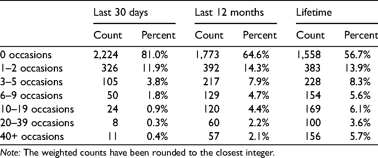
The dataset is from the Monitoring the Future project. As the largest repeated cross-sectional survey on adolescent risky behaviours (e.g., drug use and juvenile delinquency) in the United States, the Monitoring the Future project annually interviews students from hundreds of American middle and high schools (Johnston et al. 2017). Our empirical analysis was based on 12 ${}^{\mathrm{th}}$ graders ( $N$ =2,748) included in the 2018 wave of the Monitoring the Future project. One’s frequency of alcohol abuse is measured by the same question [i.e., “on how many occasions (if any) have you been drunk or very high from drinking alcoholic beverages”] and the same 7-group GRC scheme as the response category: [0 occasions, 1–2 occasions, 3–5 occasions, 6–9 occasions, 10–19 occasions, 20–39 occasions, 40+ occasions]. Yet, three reference periods (during the last 30 days, during the last 12 months, and in one’s lifetime) are used to explore frequencies of adolescent alcohol abuse, and we separately analyzed outcome variables with different reference periods to assess the performance of the FIM.

The descriptive statistics of outcome variables are shown in Table 2. As expected, respondents reported more occasions of alcohol abuse with longer reference periods. For those who were asked to report their lifetime frequencies of alcohol abuse, the specific 7-group scheme does not appear to be a preferred way to capture the full spectrum of counts because its 7 groups tend to concentrate on the lower end of the observed distribution (e.g., 0 occasions, 1–2 occasions, 3–5 occasions). Therefore, we may expect larger design errors when the frequencies of adolescent alcohol abuse have longer reference periods.

Table 2.

The weighted frequencies of being drunk or very high by different reference periods (N=2748).

	Last 30 days		Last 12 months		Lifetime
	Count	Percent	Count	Percent	Count	Percent
0 occasions	2,224	81.0%	1,773	64.6%	1,558	56.7%
1–2 occasions	326	11.9%	392	14.3%	383	13.9%
3–5 occasions	105	3.8%	217	7.9%	228	8.3%
6–9 occasions	50	1.8%	129	4.7%	154	5.6%
10–19 occasions	24	0.9%	120	4.4%	169	6.1%
20–39 occasions	8	0.3%	60	2.2%	100	3.6%
40+ occasions	11	0.4%	57	2.1%	156	5.7%

Note: The weighted counts have been rounded to the closest integer.

To compare regressor-specific design errors, we use the same set of eleven regressors (including the intercept) in both modified Poisson and ZIP models. The demographic background of respondents is indicated by female (versus male), Hispanic (versus non-Hispanic), and Black (versus non-Black). Mother’s education is an ordinal variable with the following values and categories: (1) completed grade school or less, (2) some high school, (3) completed high school, (4) some college, (5) completed college, (6) graduate or professional school after college. Here, we treat mother’s education as an ordinal variable for the sake of model parsimony (Adida et al. 2010; Martin and Shehan 1989). Mother’s full-time job is a dummy variable indicating whether a mother had full-time employment (coded as one), or part-time or no employment (coded as zero). Single-parent family means no or only one parent was present at home (coded as one) and the variable is coded as zero for intact families. GPA refers to a respondent’s grade point average in school. North-eastern, north-central, and western indicate if a school was located in the north-eastern, north-central, or western states, respectively (southern states as reference).

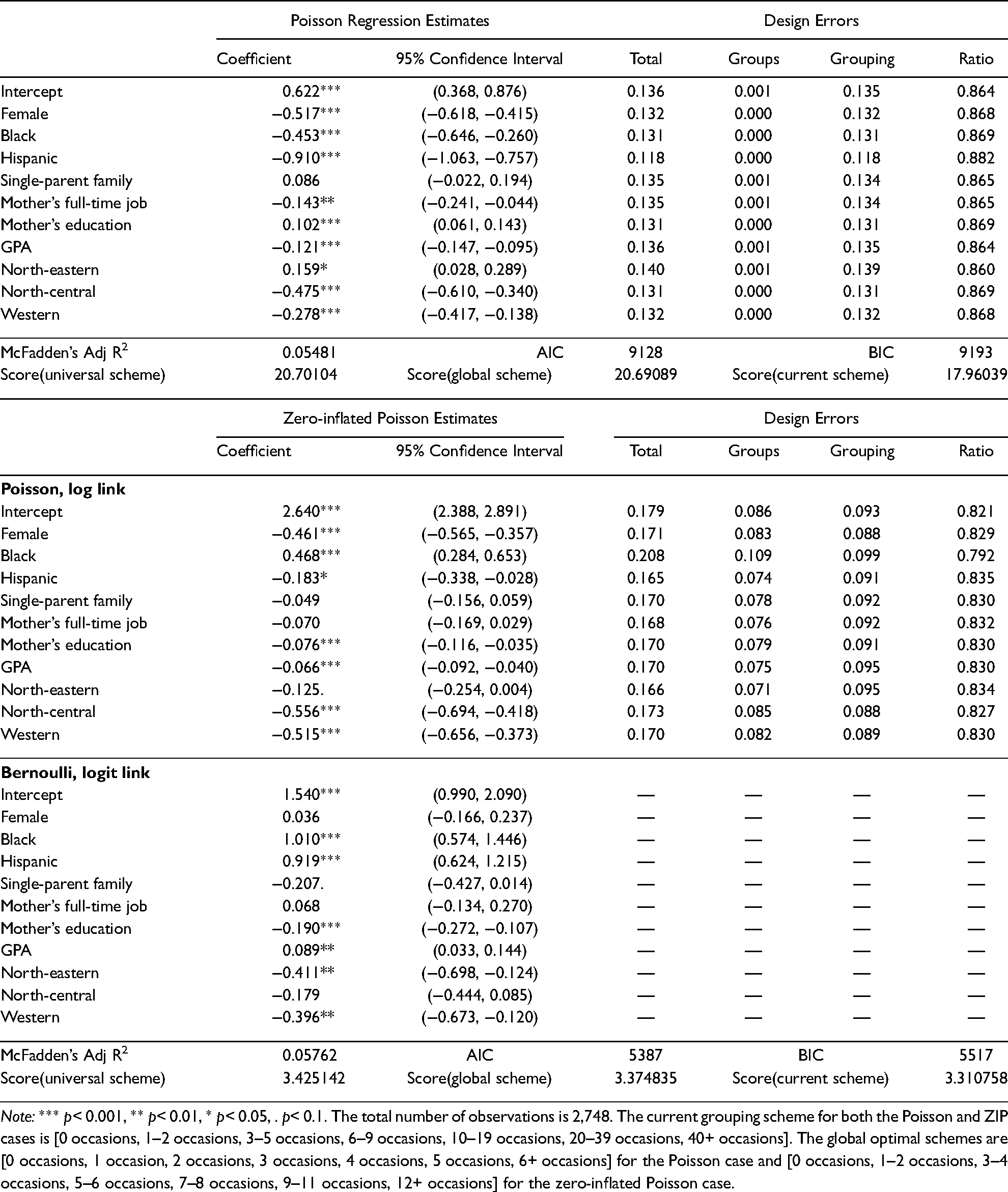
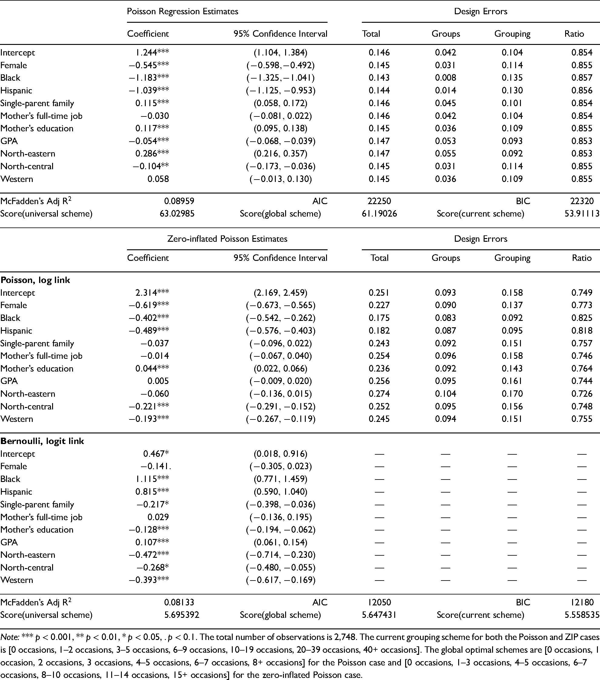
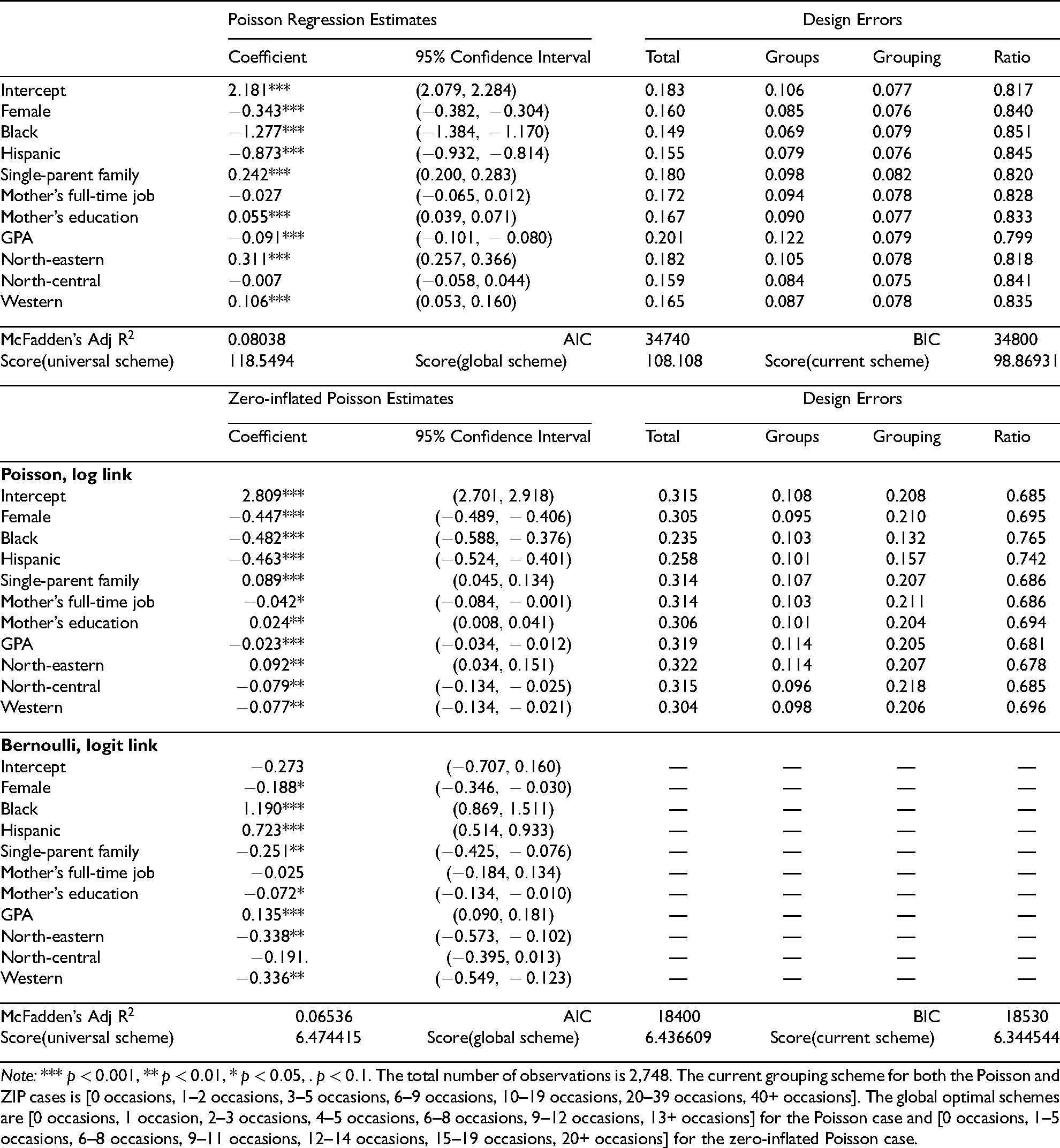
Regression estimates and regressor-specific design errors are presented in Table 3 (adolescent alcohol abuse over the last 30 days), Table 4 (adolescent alcohol abuse over the last 12 months), and Table 5 (adolescent alcohol abuse in one’s lifetime). There are several notable findings pertaining to regressor-specific design errors. First, as expected, the total design error associated with the same regressor increases when the outcome variable has a longer reference period. For example, the total design errors associated with the regressor female are 0.132, 0.145, and 0.160, when the reference periods are over the last 30 days, over the last 12 months, and in one’s lifetime, respectively. Second, based on regression estimates from generalized linear models, the FIM identifies a global 7-group optimal scheme that maximizes (a score function of) the Fisher information matrix. This global optimal grouping scheme (reported in the note below each corresponding table) allows us to decompose the total design error into the groups and grouping errors, and further assess their changes with different empirical distributions. When 7 groups are adequate to measure alcohol abuse with a shorter reference period (i.e., over the last 30 days), the groups error is negligible and the total design error is mainly attributable to the grouping error. The optimality of GRC counts can be largely achieved by replacing the current grouping scheme with a global optimal scheme, which substantially reduces, if not eliminates, the grouping error. With a longer reference period, any 7-group scheme may not provide a precise measure of observed counts despite an optimization of grouping schemes. As a result, the groups error of the same regressor increases and becomes a major source of the total error. For example, the groups error associated with GPA increases from 0.001 in Table 3 (reference period: over the last 30 days) to 0.053 in Table 4 (reference period: over the last 12 months) to 0.122 in Table 5 (reference period: in one’s life time), which contribute to 0.7%, 36.1%, and 60.7% of their corresponding total errors. Third, we calculate the (regressor-specific) ratio of $\mathrm{\Omega }({\mathcal{G}}_{\mathsf{C}},\hat{\mathit{\beta }})$ to $\mathrm{\Omega }({\mathcal{G}}_{\mathrm{\infty }},\hat{\mathit{\beta }})$ to assess the relative efficiency between the use of GRC counts and exact enumeration of counts. As suggested by these ratios in the last column of each table, the values of score functions estimated with the current 7-group GRC grouping scheme are comparable to those obtained from conventional Poisson-regression settings (all are at or above 0.8), which lend further support to the validity of the FIM and the use of GRC counts in survey research. In accordance with our discussion above, the relative efficiency associated with the same regressor tends to decrease with a longer reference period.

Table 3.

Regression estimates and design errors: alcohol abuse during last 30 days.

	Poisson Regression Estimates		Design Errors
	Coefficient	95% Confidence Interval	Total	Groups	Grouping	Ratio
Intercept	0.622***	(0.368, 0.876)	0.136	0.001	0.135	0.864
Female	−0.517***	(−0.618, −0.415)	0.132	0.000	0.132	0.868
Black	−0.453***	(−0.646, −0.260)	0.131	0.000	0.131	0.869
Hispanic	−0.910***	(−1.063, −0.757)	0.118	0.000	0.118	0.882
Single-parent family	0.086	(−0.022, 0.194)	0.135	0.001	0.134	0.865
Mother’s full-time job	−0.143**	(−0.241, −0.044)	0.135	0.001	0.134	0.865
Mother’s education	0.102***	(0.061, 0.143)	0.131	0.000	0.131	0.869
GPA	−0.121***	(−0.147, −0.095)	0.136	0.001	0.135	0.864
North-eastern	0.159*	(0.028, 0.289)	0.140	0.001	0.139	0.860
North-central	−0.475***	(−0.610, −0.340)	0.131	0.000	0.131	0.869
Western	−0.278***	(−0.417, −0.138)	0.132	0.000	0.132	0.868
McFadden’s Adj R2	0.05481	AIC	9128	BIC		9193
Score(universal scheme)	20.70104	Score(global scheme)	20.69089	Score(current scheme)		17.96039
	Zero-inflated Poisson Estimates		Design Errors
	Coefficient	95% Confidence Interval	Total	Groups	Grouping	Ratio
Poisson, log link
Intercept	2.640***	(2.388, 2.891)	0.179	0.086	0.093	0.821
Female	−0.461***	(−0.565, −0.357)	0.171	0.083	0.088	0.829
Black	0.468***	(0.284, 0.653)	0.208	0.109	0.099	0.792
Hispanic	−0.183*	(−0.338, −0.028)	0.165	0.074	0.091	0.835
Single-parent family	−0.049	(−0.156, 0.059)	0.170	0.078	0.092	0.830
Mother’s full-time job	−0.070	(−0.169, 0.029)	0.168	0.076	0.092	0.832
Mother’s education	−0.076***	(−0.116, −0.035)	0.170	0.079	0.091	0.830
GPA	−0.066***	(−0.092, −0.040)	0.170	0.075	0.095	0.830
North-eastern	−0.125.	(−0.254, 0.004)	0.166	0.071	0.095	0.834
North-central	−0.556***	(−0.694, −0.418)	0.173	0.085	0.088	0.827
Western	−0.515***	(−0.656, −0.373)	0.170	0.082	0.089	0.830
Bernoulli, logit link
Intercept	1.540***	(0.990, 2.090)	—	—	—	—
Female	0.036	(−0.166, 0.237)	—	—	—	—
Black	1.010***	(0.574, 1.446)	—	—	—	—
Hispanic	0.919***	(0.624, 1.215)	—	—	—	—
Single-parent family	−0.207.	(−0.427, 0.014)	—	—	—	—
Mother’s full-time job	0.068	(−0.134, 0.270)	—	—	—	—
Mother’s education	−0.190***	(−0.272, −0.107)	—	—	—	—
GPA	0.089**	(0.033, 0.144)	—	—	—	—
North-eastern	−0.411**	(−0.698, −0.124)	—	—	—	—
North-central	−0.179	(−0.444, 0.085)	—	—	—	—
Western	−0.396**	(−0.673, −0.120)	—	—	—	—
McFadden’s Adj R2	0.05762	AIC	5387	BIC		5517
Score(universal scheme)	3.425142	Score(global scheme)	3.374835	Score(current scheme)		3.310758

Note: *** p< 0.001, ** p< 0.01, * p< 0.05, . p< 0.1. The total number of observations is 2,748. The current grouping scheme for both the Poisson and ZIP cases is [0 occasions, 1–2 occasions, 3–5 occasions, 6–9 occasions, 10–19 occasions, 20–39 occasions, 40+ occasions]. The global optimal schemes are [0 occasions, 1 occasion, 2 occasions, 3 occasions, 4 occasions, 5 occasions, 6+ occasions] for the Poisson case and [0 occasions, 1–2 occasions, 3–4 occasions, 5–6 occasions, 7–8 occasions, 9–11 occasions, 12+ occasions] for the zero-inflated Poisson case.

Table 4.

Regression estimates and design errors: alcohol abuse during last 12 months.

	Poisson Regression Estimates		Design Errors
	Coefficient	95% Confidence Interval	Total	Groups	Grouping	Ratio
Intercept	$1.244$ ***	$(1.104,1.384)$	0.146	0.042	0.104	0.854
Female	$-0.545$ ***	$(-0.598,-0.492)$	0.145	0.031	0.114	0.855
Black	$-1.183$ ***	$(-1.325,-1.041)$	0.143	0.008	0.135	0.857
Hispanic	$-1.039$ ***	$(-1.125,-0.953)$	0.144	0.014	0.130	0.856
Single-parent family	$0.115$ ***	$(0.058,0.172)$	0.146	0.045	0.101	0.854
Mother’s full-time job	$-0.030$	$(-0.081,0.022)$	0.146	0.042	0.104	0.854
Mother’s education	$0.117$ ***	$(0.095,0.138)$	0.145	0.036	0.109	0.855
GPA	$-0.054$ ***	$(-0.068,-0.039)$	0.147	0.053	0.093	0.853
North-eastern	$0.286$ ***	$(0.216,0.357)$	0.147	0.055	0.092	0.853
North-central	$-0.104$ **	$(-0.173,-0.036)$	0.145	0.031	0.114	0.855
Western	$0.058$	$(-0.013,0.130)$	0.145	0.036	0.109	0.855
McFadden’s Adj R ${}^2$	0.08959	AIC	22250	BIC		22320
Score(universal scheme)	63.02985	Score(global scheme)	61.19026	Score(current scheme)		53.91113
	Zero-inflated Poisson Estimates		Design Errors
	Coefficient	95% Confidence Interval	Total	Groups	Grouping	Ratio
Poisson, log link
Intercept	$2.314$ ***	$(2.169,2.459)$	0.251	0.093	0.158	0.749
Female	$-0.619$ ***	$(-0.673,-0.565)$	0.227	0.090	0.137	0.773
Black	$-0.402$ ***	$(-0.542,-0.262)$	0.175	0.083	0.092	0.825
Hispanic	$-0.489$ ***	$(-0.576,-0.403)$	0.182	0.087	0.095	0.818
Single-parent family	$-0.037$	$(-0.096,0.022)$	0.243	0.092	0.151	0.757
Mother’s full-time job	$-0.014$	$(-0.067,0.040)$	0.254	0.096	0.158	0.746
Mother’s education	$0.044$ ***	$(0.022,0.066)$	0.236	0.092	0.143	0.764
GPA	$0.005$	$(-0.009,0.020)$	0.256	0.095	0.161	0.744
North-eastern	$-0.060$	$(-0.136,0.015)$	0.274	0.104	0.170	0.726
North-central	$-0.221$ ***	$(-0.291,-0.152)$	0.252	0.095	0.156	0.748
Western	$-0.193$ ***	$(-0.267,-0.119)$	0.245	0.094	0.151	0.755
Bernoulli, logit link
Intercept	$0.467$ *	$(0.018,0.916)$	—	—	—	—
Female	$-0.141$ .	$(-0.305,0.023)$	—	—	—	—
Black	$1.115$ ***	$(0.771,1.459)$	—	—	—	—
Hispanic	$0.815$ ***	$(0.590,1.040)$	—	—	—	—
Single-parent family	$-0.217$ *	$(-0.398,-0.036)$	—	—	—	—
Mother’s full-time job	$0.029$	$(-0.136,0.195)$	—	—	—	—
Mother’s education	$-0.128$ ***	$(-0.194,-0.062)$	—	—	—	—
GPA	$0.107$ ***	$(0.061,0.154)$	—	—	—	—
North-eastern	$-0.472$ ***	$(-0.714,-0.230)$	—	—	—	—
North-central	$-0.268$ *	$(-0.480,-0.055)$	—	—	—	—
Western	$-0.393$ ***	$(-0.617,-0.169)$	—	—	—	—
McFadden’s Adj R ${}^2$	0.08133	AIC	12050	BIC		12180
Score(universal scheme)	5.695392	Score(global scheme)	5.647431	Score(current scheme)		5.558535

Note: *** $p<0.001$ , ** $p<0.01$ , * $p<0.05$ , . $p<0.1$ . The total number of observations is 2,748. The current grouping scheme for both the Poisson and ZIP cases is [0 occasions, 1–2 occasions, 3–5 occasions, 6–9 occasions, 10–19 occasions, 20–39 occasions, 40+ occasions]. The global optimal schemes are [0 occasions, 1 occasion, 2 occasions, 3 occasions, 4–5 occasions, 6–7 occasions, 8+ occasions] for the Poisson case and [0 occasions, 1–3 occasions, 4–5 occasions, 6–7 occasions, 8–10 occasions, 11–14 occasions, 15+ occasions] for the zero-inflated Poisson case.

Table 5.

Regression estimates and design errors: alcohol abuse in one’s lifetime.

	Poisson Regression Estimates		Design Errors
	Coefficient	95% Confidence Interval	Total	Groups	Grouping	Ratio
Intercept	$2.181$ ***	$(2.079,2.284)$	0.183	0.106	0.077	0.817
Female	$-0.343$ ***	$(-0.382,-0.304)$	0.160	0.085	0.076	0.840
Black	$-1.277$ ***	$(-1.384,-1.170)$	0.149	0.069	0.079	0.851
Hispanic	$-0.873$ ***	$(-0.932,-0.814)$	0.155	0.079	0.076	0.845
Single-parent family	$0.242$ ***	$(0.200,0.283)$	0.180	0.098	0.082	0.820
Mother’s full-time job	$-0.027$	$(-0.065,0.012)$	0.172	0.094	0.078	0.828
Mother’s education	$0.055$ ***	$(0.039,0.071)$	0.167	0.090	0.077	0.833
GPA	$-0.091$ ***	$(-0.101,-0.080)$	0.201	0.122	0.079	0.799
North-eastern	$0.311$ ***	$(0.257,0.366)$	0.182	0.105	0.078	0.818
North-central	$-0.007$	$(-0.058,0.044)$	0.159	0.084	0.075	0.841
Western	$0.106$ ***	$(0.053,0.160)$	0.165	0.087	0.078	0.835
McFadden’s Adj R ${}^2$	0.08038	AIC	34740	BIC		34800
Score(universal scheme)	118.5494	Score(global scheme)	108.108	Score(current scheme)		98.86931
	Zero-inflated Poisson Estimates		Design Errors
	Coefficient	95% Confidence Interval	Total	Groups	Grouping	Ratio
Poisson, log link
Intercept	$2.809$ ***	$(2.701,2.918)$	0.315	0.108	0.208	0.685
Female	$-0.447$ ***	$(-0.489,-0.406)$	0.305	0.095	0.210	0.695
Black	$-0.482$ ***	$(-0.588,-0.376)$	0.235	0.103	0.132	0.765
Hispanic	$-0.463$ ***	$(-0.524,-0.401)$	0.258	0.101	0.157	0.742
Single-parent family	$0.089$ ***	$(0.045,0.134)$	0.314	0.107	0.207	0.686
Mother’s full-time job	$-0.042$ *	$(-0.084,-0.001)$	0.314	0.103	0.211	0.686
Mother’s education	$0.024$ **	$(0.008,0.041)$	0.306	0.101	0.204	0.694
GPA	$-0.023$ ***	$(-0.034,-0.012)$	0.319	0.114	0.205	0.681
North-eastern	$0.092$ **	$(0.034,0.151)$	0.322	0.114	0.207	0.678
North-central	$-0.079$ **	$(-0.134,-0.025)$	0.315	0.096	0.218	0.685
Western	$-0.077$ **	$(-0.134,-0.021)$	0.304	0.098	0.206	0.696
Bernoulli, logit link
Intercept	$-0.273$	$(-0.707,0.160)$	—	—	—	—
Female	$-0.188$ *	$(-0.346,-0.030)$	—	—	—	—
Black	$1.190$ ***	$(0.869,1.511)$	—	—	—	—
Hispanic	$0.723$ ***	$(0.514,0.933)$	—	—	—	—
Single-parent family	$-0.251$ **	$(-0.425,-0.076)$	—	—	—	—
Mother’s full-time job	$-0.025$	$(-0.184,0.134)$	—	—	—	—
Mother’s education	$-0.072$ *	$(-0.134,-0.010)$	—	—	—	—
GPA	$0.135$ ***	$(0.090,0.181)$	—	—	—	—
North-eastern	$-0.338$ **	$(-0.573,-0.102)$	—	—	—	—
North-central	$-0.191$ .	$(-0.395,0.013)$	—	—	—	—
Western	$-0.336$ **	$(-0.549,-0.123)$	—	—	—	—
McFadden’s Adj R ${}^2$	0.06536	AIC	18400	BIC		18530
Score(universal scheme)	6.474415	Score(global scheme)	6.436609	Score(current scheme)		6.344544

Note: *** $p<0.001$ , ** $p<0.01$ , * $p<0.05$ , . $p<0.1$ . The total number of observations is 2,748. The current grouping scheme for both the Poisson and ZIP cases is [0 occasions, 1–2 occasions, 3–5 occasions, 6–9 occasions, 10–19 occasions, 20–39 occasions, 40+ occasions]. The global optimal schemes are [0 occasions, 1 occasion, 2–3 occasions, 4–5 occasions, 6–8 occasions, 9–12 occasions, 13+ occasions] for the Poisson case and [0 occasions, 1–5 occasions, 6–8 occasions, 9–11 occasions, 12–14 occasions, 15–19 occasions, 20+ occasions] for the zero-inflated Poisson case.

As noted in our discussion of Table 1, design errors associated with the binomial part of a modified ZIP model are trivial so we focus on design errors associated with the Poisson part. Given that only a proportion of respondents are exposed to the risk of alcohol abuse under a ZIP model, its estimated average frequency $\lambda$ is expected to be higher than that estimated from a Poisson regression model. Consequently, with a larger $\lambda$ estimated from the modified ZIP model, the 7-group GRC scheme does not provide an adequate measure of observed counts. For the same regressor, we observe larger design errors and lower relative efficiencies (as indicated by ratios of $\mathrm{\Omega }({\mathcal{G}}_{\mathsf{C}},\hat{\mathit{\beta }})$ to $\mathrm{\Omega }({\mathcal{G}}_{\mathrm{\infty }},\hat{\mathit{\beta }})$ ) in the Poisson part of a modified ZIP model than their counterparts in a modified Poisson regression model. These regressor-specific design errors also allow us to compute effective sample sizes associated with different variables in this empirical setting. For example, the calculated groups and grouping errors associated with the intercept of the Poisson part in Table 4 are 0.042 and 0.104, respectively. According to (11), we have $\frac{n_{\mathsf{L}}}{n_{\mathsf{C}}}$ as 0.891. In other words, if the optimum design of survey counts were considered by survey investigators, it can save about 11% of the sample size to reach the same efficiency for the estimation of the intercept.

According to regression estimates, females, Hispanics, and students with higher GPAs reported lower frequencies of alcohol abuse than their counterparts did. Adolescents from single-parent families or north-eastern states (versus those in southern states) had higher frequencies of alcohol abuse. Yet, the impacts of race and mother’s socioeconomic status on adolescent alcohol abuse are mixed. Results from the binomial part of the modified ZIP models suggest that African Americans, Hispanics, students with better school performance, and students from intact families have significantly less exposure to alcohol abuse. As expected, measures of goodness of fit, such as Akaike information criterion (AIC) and Bayesian information criterion (BIC), favor a modified ZIP model over a corresponding modified Poisson model.

Discussion

Counts are often grouped and/or right-censored in survey instruments to study a wide range of behavioural, attitudinal, and event frequencies, especially when concerning sensitive research topics, vulnerable populations, or respondents with less cognitive capacities. Yet, grouping and right-censoring also pose major difficulties in survey methodology and statistical analysis. The optimum design of survey counts and its impacts on statistical analysis have not been systematically investigated by researchers. Despite the recent advances in designing and modeling GRC counts, existing studies fail to address the intrinsic link between the design and analysis of survey counts in a regression setting. As a result, after survey investigators decide to choose GRC response categories, their grouping and right-censoring decisions are often subjective due to the absence of a yardstick against which the performance of a GRC grouping scheme in statistical analysis can be assessed.

To develop a unified framework for assessing and analyzing GRC counts in a regression setting, we begin with modified Poisson models to conceptualize GRC counts and then describe in detail the definition, decomposition, and optimization of their regressor-specific design errors. We further demonstrate how the optimum design of survey counts can be informed by generalized linear models. In particular, we develop a novel search algorithm, the FIM, to process infinitely many grouping schemes and identify a global optimal grouping scheme maximizing the Fisher information matrices of the modified Poisson estimates. By doing so, the global optimal grouping scheme reduces the grouping error to zero. The unified framework makes the calculation of regressor-specific design errors possible, which clearly provides a powerful tool for assessing the performance of a specific GRC grouping scheme in empirical research. The validity of this unified framework is corroborated by results from both simulation and empirical studies. This study suggests that, with the optimum design of survey counts, the performance of modified Poisson estimators based on GRC counts is comparable to that of conventional Poisson estimators based on the exact enumeration of counts. The optimum design is able to achieve the same estimation efficiency with a smaller sample size.

Survey design is an iterative and interactive multi-purpose optimization process (Biemer 2010; Groves et al. 2009; Schaeffer and Dykema 2011). The minimization of design errors is not the sole principle for designing response categories; rather, survey investigators need to consider various factors such as the consistency of response categories over years, the comparability of survey estimates across studies and survey questions, and answering strategies adopted by respondents (Gehlbach and Barge 2012; Schaeffer and Dykema 2020, 2011). Since design errors are an essential component of this multi-purpose optimization process, it is not the presence of design errors but the absence of a tool for assessing design errors that scholars should be concerned about and continue to work on. Without such a tool, it is difficult if not impossible for survey investigators to tell how good (or bad) their design is, adjust their survey design, or allocate resources or budgets to where they are most needed (Biemer 2010). This study not only provides a powerful tool for assessing the design errors of survey counts, but also offers an integrated perspective from which to unify survey design and statistical analysis before, during, and after data collection.