Sage Journals: Discover world-class research

Abstract

This article provides a meta-analysis of studies using the crosswise model (CM) in estimating the prevalence of sensitive characteristics in different samples and populations. On a data set of 141 items published in 33 either articles or books, we compare the difference (Δ) between estimates based on the CM and a direct question (DQ). The overall effect size of Δ is 4.88; 95% CI [4.56, 5.21]. The results of a meta-regression indicate that Δ is smaller when general populations and nonprobability samples are considered. The population effect suggests an education effect: Differences between the CM and DQ estimates are more likely to occur when highly educated populations, such as students, are studied. Our findings raise concerns to what extent the CM is able to improve estimates of sensitive behavior in general population samples.

Keywords

sensitive characteristics social desirability sampling RRT WEIRD

Introduction

Reporting sensitive attitudes or behavior in surveys is prone to social desirability bias, that is, respondents’ tendency to overreport socially desirable and to underreport socially undesirable behavior, attitudes, or characteristics (Bradburn, Sudman, and Wansink 2004; Phillips and Clancy 1972; Thomas et al. 2017; Tourangeau, Rips, and Rasinski 2000). Different indirect question formats have been developed to protect survey respondents’ responses when they are asked about sensitive items. Randomized response techniques (RRTs) are one popular approach (Krumpal et al. 2015; Warner 1965). RRTs traditionally rely on randomization devices, such as coins or dice, to obscure respondents’ answers in a way that it is impossible to identify their true status of the sensitive characteristics. However, researchers are able to estimate the prevalence of the sensitive item relying on elementary probability theory because the randomization device has known probabilities (Boruch 1971; Greenberg et al. 1969; Horvitz, Simmons, and Shah 1968; Kuk 1990; Warner 1965). Yet, one major drawback of most RRTs is that respondents may refuse to answer a particular question, break off the survey interview, or give dishonest or self-protective answers because they are suspicious of the unusual question format and complex instructions (Krumpal et al. 2015; Ulrich et al. 2012).

The crosswise model (CM) has been developed to overcome the issues of using a randomization device (Yu, Tian, and Tang 2008). More specifically, survey respondents are asked to answer two questions—an unobtrusive one with known probabilities and a sensitive one—but to provide only one joint answer to the combination of both of these questions (Höglinger, Jann, and Diekmann 2016; Korndörfer, Krumpal, and Schmukle 2014; Ulrich et al. 2012). As the CM includes a question with known probabilities, it is possible to estimate the prevalence of the sensitive characteristic but without imposing an additional task on the survey respondents. The technique has been implemented in a variety of different social science research studies since its development. While some criticism has been raised about the method (Höglinger et al. 2016; Höglinger and Jann 2018; Jerke et al. 2019), a systematic review of the CM is still outstanding.

We begin by presenting the logic and derivation of the CM, followed by a discussion of the potential effects that this question format may introduce with regard to the quality of the final survey estimate. Next, we conduct a systematic review of the difference ( $Δ$ ) of the CM and the DQ estimates in all available publications (n_p = 33, including $n_{i} = 141$ items). Meta-analysis of all eligible items (n_p = 25, including $n_{i} = 104$ items) allows us to further assess the effects of the survey design on the results of previous research using the CM. We close with a discussion of our findings and their implications for practical applications of the CM.

Estimating Sensitive Characteristics Using the CM

The CM asks two simple yes/no-questions: An unobtrusive question with known probabilities (Y) and a sensitive one with unknown probabilities (X) (Tan, Tian, and Tang 2009; Yu et al. 2008). Respondents are instructed to give a joint answer to the two questions instead of answering each question individually. The available response options only indicate that the answer to both questions is the same (A) or that the answer to both questions is different (B) (see Table 1).

Table 1.

Response Options in the Crosswise Model.

	$Y = 0$	$Y = 1$
$X = 0$	A	B
$X = 1$	B	A

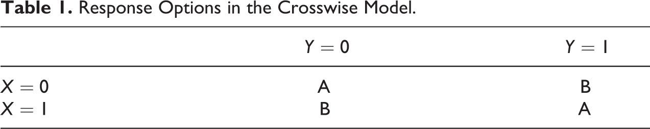
If (1) both answers are captured by dichotomous response codes, (2) the unobtrusive behavior has a known probability p, and is (3) unrelated to the sensitive one, it is possible to estimate the prevalence of the sensitive item (Yu et al. 2008). For example, the unobtrusive question could ask whether a particular person was born in October, November, or December. 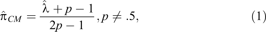The probability of being born in these months is approximately $p = .25$ , given an assumed uniform birthday distribution. The prevalence of the sensitive behavior $π$ can then be estimated by

{\hat{π}}_{C M} = \frac{\hat{λ} + p - 1}{2 p - 1}, p \neq .5,

where p is the known population prevalence of the unobtrusive item (in the birthday example approximately $p = .25$ ) and $\hat{λ}$ is the proportion of respondents giving the same answer to both questions in the CM. The sampling variance (Yu et al. 2008) $Var ({\hat{π}}_{CM})$ is given by:

Var ({\hat{π}}_{CM}) = \frac{\hat{λ} (1 - \hat{λ})}{n {(2 p - 1)}^{2}} = \frac{{\hat{π}}_{CM} (1 - {\hat{π}}_{CM})}{n} + \frac{p (1 - p)}{n {(2 p - 1)}^{2}}, p \neq .5.

Respondents should experience more confidentiality in their responses by the question design because survey interviewers and data users are unable to identify the responses to the individual questions. The CM could thus be an attractive method for interviewer-administered but also for self-administered modes of data collection, as the technique does not require any additional randomization devices (Krumpal 2013; Yu et al. 2008). While the CM seems to have benefits in eliciting sensitive characteristics, its estimates are associated with larger standard errors and wider confidence intervals. To achieve similar precision as a direct question (DQ) format, the CM thus requires larger sample sizes (Ulrich et al. 2012).

Previous studies suggest that the CM effectively reduces misreporting of sensitive behaviors (inter alia Coutts et al. 2011; Enzmann et al. 2018; Hoffmann and Musch 2016; Höglinger and Jann 2018; Jann, Jerke, and Krumpal 2012; Korndörfer et al. 2014; Krumpal 2012; Kundt 2014). However, it is noteworthy that many of these CM results seem to rely on homogeneous, nonprobability samples that include respondents with high cognitive abilities, such as students. Krosnick (1991) suggested that bias in survey responses may vary across respondents with different cognitive abilities. This will be especially relevant for questions that impose a higher cognitive burden on respondents by design, such as RRTs and the CM (Jerke et al. 2019; Schnell, Hill, and Esser 1988, Schnell, Thomas, and Noack 2019). Thus, we hypothesize that the effectiveness of the CM may depend on respondents’ abilities and should thus depend on the target population and the sample quality of a survey.

Potential Effects of the CM on the Final Survey Estimates

The total survey error (TSE; Andersen, Kasper, and Frankel 1979; Groves and Lyberg 2010; Weissberg 2009) posits that a survey estimate is influenced by potential representation and measurement error. While the former includes sampling and nonsampling errors, the latter refers to all influences that may affect the accuracy of the measured concept.

Representation error depends on the sample type, with probability samples resulting in more accurate estimates as coverage, sampling, and nonresponse errors are minimized (Cornesse et al. 2020). By contrast, nonprobability samples lack the probability mechanism, and it has been recommended to report the results based on nonprobability samples as “indications” rather than estimates (Baker et al. 2013; Matthews 2008). For example, especially web surveys recruited on the basis of self-recruitment into access panels, such as Amazon Mechanical Turk, have been found to be biased by well-educated and (politically) more interested, professional survey respondents.¹ Moreover, we expect that the specific sample composition of nonprobability samples may affect the performance of special question techniques (Schnell et al. 1988). Little research has explored how well survey respondents understand the CM, some evidence indicates that it is harder to cognitively process the CM’s question wording (Jerke et al. 2019).

Similarly, it can be difficult to disentangle the effects of education and motivation in nonprobability samples or samples recruiting special populations, such as students. With regard to the latter, educational effects are obvious and inevitable. For the former, we should observe a similar effect, given self-recruited individuals have been found to be more interested and have higher cognitive abilities in comparison to samples that include the general population. These samples have been described by Henrich and coauthors as Western, Educated, Industrialized, Rich, and Democratic (WEIRD; Henrich, Heine, and Norenzayan 2010a, 2010b) populations. Due to an increasing educational heterogeneity, we expect the difference ( $Δ$ ) between the CM and DQ estimates to be smaller when general populations are concerned and larger for WEIRD subjects and nonprobability samples.

The objective of the CM is to reduce the risk of social desirability bias. For socially undesirable items, higher proportions in the CM condition are considered to be better estimates because they arguably reflect the unknown “true” status more accurately than the DQ according to the “more-is-better” assumption (Cannell, Oksenberg, and Converse 1977; Cannell, Miller, and Oksenberg 1981; Lensvelt-Mulders et al. 2005; Umesh and Peterson 1991). By contrast, respondents are believed to overreport socially desirable characteristics, which should result in a lower prevalence estimate in the CM condition compared to the DQ.

Previous research suggested the “more-is-better” assumption might be undermined by a respondent’s interpretation of what is desirable or undesirable, resulting in subgroups differences (Smith 1992). For example, in a study of imprisonment by Maxfield, Weiler, and Widom (2000), 21 percent falsely reported that they have been imprisoned but have never been arrested. Thus, overreporting might be the result of respondents not comprehending or following the instructions of the question correctly, thus giving an inaccurate answer or deliberately providing an inaccurate answer. These mechanisms may result in false-positives answers (Höglinger and Diekmann 2017; Höglinger and Jann 2018; Jerke et al. 2019). Although we acknowledge the possibility of different subgroup interpretations of social desirability resulting in false-positives and a violation of the “more-is-better” assumption, the discussion of these problems is beyond the scope of this article. As a large body of the literature still relies on this assumption when using RRT, in general, or the CM, in particular, it is yet important to investigate the difference in estimates based on the CM and the DQ.

Empirical Studies Using the CM

Following the guidelines on Preferred Reporting of Items for Systematic Reviews and Meta-Analyses (Moher et al. 2009), we reviewed all empirical studies on the CM published by February 2020. Our search was conducted using four large and commonly used databases for academic publications in survey methodology (Web of Science, Google Scholar, PubMed, and ScienceOpen). The number of publications included in the systematic review is 33 (n_p = 33), including 141 items (n_i = 141)² estimating proportions of sensitive characteristics using the CM and comparing them to DQ. 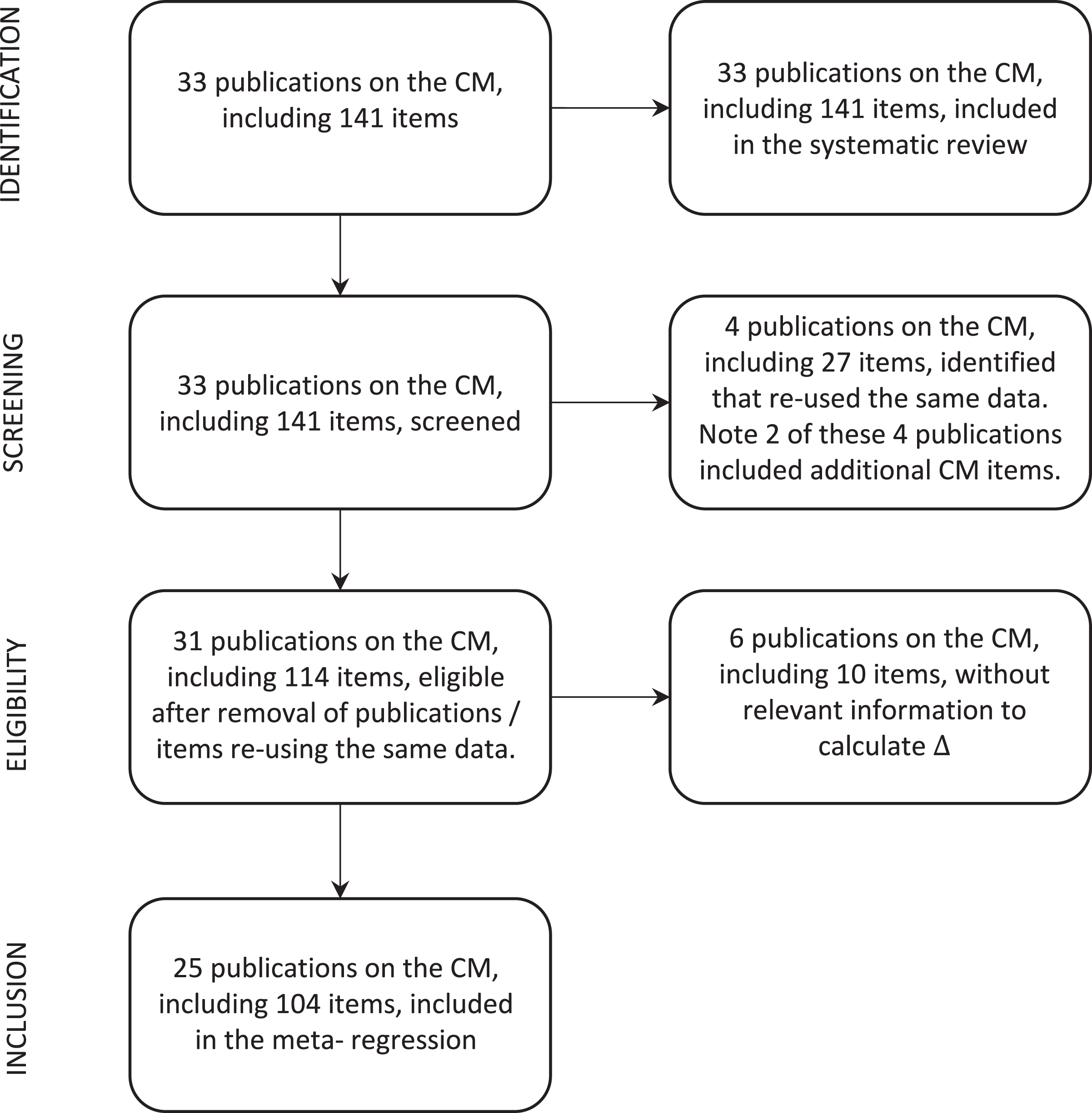If the authors reported the difference in the prevalence estimates of the CM and DQ, we include the reported estimates in our analysis.³ Four publications with 27 items include results that have already been published elsewhere, at least partially.⁴ Six publications, including 10 items, did not report the necessary information to calculate $Δ$ of the CM and DQ estimate and its standard error (Klimas et al. 2019; Nakhaee, Pakravan, and Nakhaee 2013; Schnapp 2019; Vakilian et al. 2014, 2016, 2019).⁵ We drop these 27 items from the meta-analysis and only keep the items included in the initial publications. For all other items, the relevant estimates were either accurately reported or sufficient information was accessible in supplementary materials or provided by email, so that we were able to compute the necessary statistics. As noted earlier, all items (n_p = 33, n_i = 141) are considered in the systematic review. The total number of items for the empirical analysis is smaller (n_p = 25, n_i = 104; see Figure 1).

Figure 1.

Selection process of crosswise model studies for inclusion in the systematic review and meta-analysis.

Of the included CM items, a majority have been implemented to capture socially undesirable behavior or attitudes (n_i = 135 items). For example, the CM has been applied to estimate plagiarism (Coutts et al. 2011; Hoffmann et al. 2015; Höglinger et al. 2016; Hopp and Speil 2018; Jann et al. 2012), substance abuse (Banayejeddi et al. 2019; Höglinger and Diekmann 2017; Höglinger et al. 2016; Nakhaee et al. 2013; Shamsipour et al. 2014), risky sexual behavior (Klimas et al. 2019; Nasirian et al. 2018; Safiri et al. 2018; Vakilian et al. 2019; Vakilian et al. 2014, 2016), carrying rare diseases (Höglinger and Diekmann 2017; Schnapp 2019), tax/fee evasion and corruption (Corbacho et al. 2016; Gingerich et al. 2016; Höglinger and Jann 2018; Hopp and Speil 2018; Korndörfer et al. 2014; Kundt 2014; Kundt, Misch, and Nerré 2016; Oliveros and Gingerich 2019), nonvoting (Höglinger and Jann 2018), radical right voting (Gschwend, Juhl, and Lehrer 2018; Lehrer, Juhl, and Gschwend 2019), antisocial behavior (Enzmann 2017; Enzmann et al. 2018; Höglinger and Jann 2018), as well as prejudice, Xenophobia, and Islamophobia (Hoffmann and Musch 2016, 2019; Johann and Thomas 2017). However, little research has applied the CM to estimate socially desirable behavior, such as self-reported blood and organ donations (Höglinger and Diekmann 2017; Walzenbach and Hinz 2019).⁶

We also coded the sample type, referring to probability versus nonprobability samples. A majority of the CM items (n_i = 89; 63 percent) has been implemented on nonprobability samples (Coutts et al. 2011; Gschwend et al. 2018; Hoffmann et al. 2015; Hoffmann et al. 2017; Hoffmann and Musch 2016; Höglinger et al. 2016; Höglinger and Jann 2018; Hopp and Speil 2018; Jann et al. 2012; Johann and Thomas 2017; Korndörfer et al. 2014; Kundt 2014; Kundt et al. 2016; Nakhaee et al. 2013; Shamsipour et al. 2014; Vakilian et al. 2014, 2016; Waubert de Puiseau, Hoffmann, and Musch 2017), only 52 items in 8 publications are based on samples drawn on the basis of probability methods (Corbacho et al. 2016; Enzmann et al. 2018; Enzmann 2017; Gingerich et al. 2016; Gschwend et al. 2018; Lehrer et al. 2019; Oliveros and Gingerich 2019; Schnell et al. 2019).⁷

A majority of items were drawn from studies involving WEIRD samples (n_i = 119, 84 percent). This includes n_i = 105 (74 percent) students samples and n_i = 14 (10 percent) other WEIRD subjects. Only 22 items in 10 different publications (16 percent) rely on general populations.⁸

Systematic Review of CM Studies

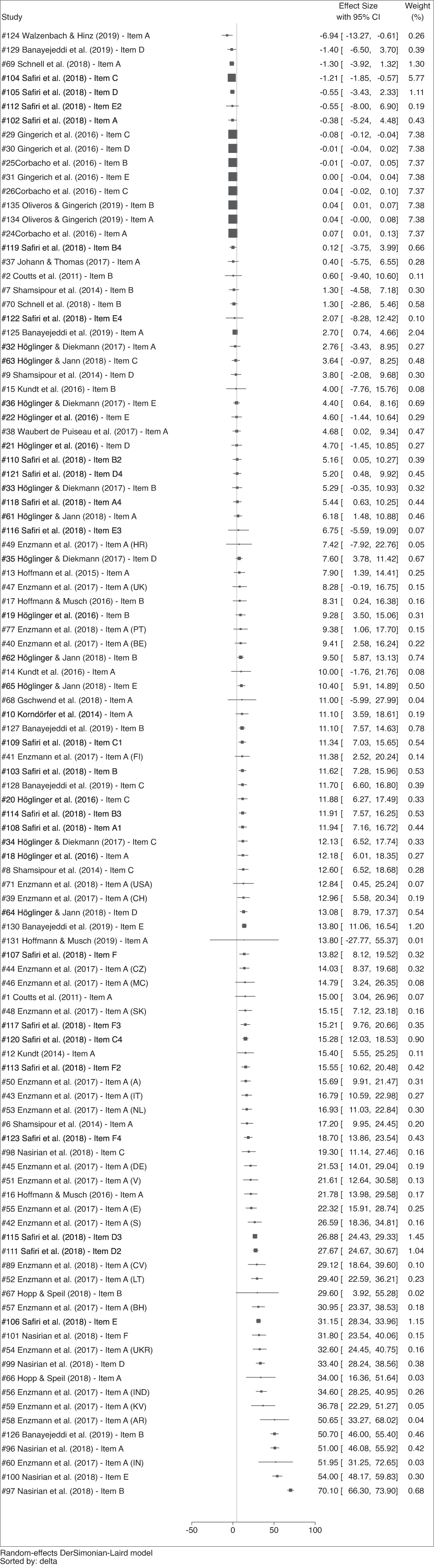
A forest plot (Palmer and Sterne 2009) of all items, for which $Δ$ and its standard error were available or could be calculated, is displayed in Figure 2 (n_i = 104). The plot is arranged by effect size of $Δ$ . The figure demonstrates that 29 of the 104 items have 95% confidence intervals (CI) around $Δ$ that include zero, indicating nonsignificant differences of the CM and DQ estimates at conventional levels.⁹ The remaining 75 items have a confidence interval of the difference between the CM and DQ that does not include zero.¹⁰

Figure 2.

Forest plot organized by effect size, restricted sample (n_i = 104).

We present a plot of the overall effects size and the prediction interval in Figure 3. The overall effect size is 4.88; 95% CI [4.56, 5.21]. It was calculated employing the DerSimonion–Laird random effects estimator (DerSimonian and Laird 1986) and is represented in Figure 3 by the narrow grey diamond and whiskers. Although the effect is statistically significant at conventional levels, the overall effect size is small.¹¹ The 95% prediction interval (Borenstein et al. 2009) [95% PI: 3.616, 6.153] is represented by the hollow diamond in the Figure 3 and indicates the plausible range for the effect size in a future study.

Figure 3.

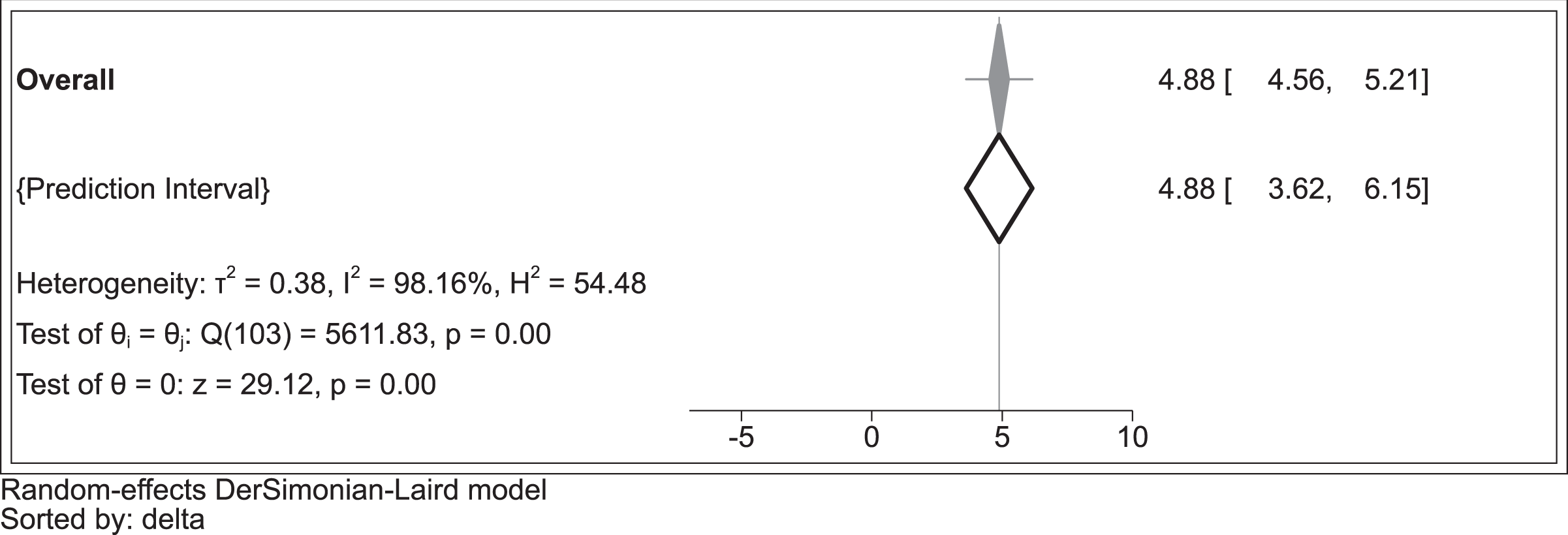
Overall effect size (4.88 [4.56, 5.21]) and prediction interval [3.616; 6.153], restricted sample (n_i = 104).

Previous research suggest that between-study variation could cause bias (Borenstein 2019). To control for this factor, we estimated three indicators of study heterogeneity: Cochran’s Q, I ², and $τ^{2}$ . While Cochran’s Q is sensitive to the number of studies and the study size, Higgins and Thompson (2002) suggested to also report I ², which is not sensitive to the number of studies but to the study size. By contrast, $τ^{2}$ is neither sensitive to the number of studies included nor to the study size (Schwarzer, Carpenter, and Rücker 2015). Table 2 summarizes the results for the full sample and subgroups for population and sample type.

Table 2.

Heterogeneity Tests. Restricted Sample.

	Q	df	I ²	$τ^{2}$	$χ^{2}$
Overall	5,611.83**	103	98.16%	0.38
WEIRD population	4,071.05**	88	97.84%	222.61
General population	54.02**	14	74.08%	0.000
Difference					93.88**
Nonprobability	4,871.30**	74	98.48%	0.33
Probability	378.10**	28	92.59%	157.94
Difference					33.30**

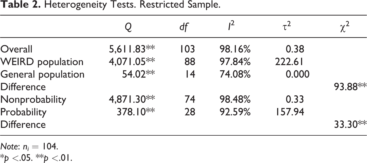
Note: n_i = 104.

*p $<$ .05. **p $<$ .01.

The results in Table 2 indicate study heterogeneity for the overall sample. This is shown by the statistically significant coefficient of Cochran’s Q and the high ratio of I ² in the top row. Moreover, $τ^{2}$ suggest at least some variation due to study heterogeneity. It is important to note, however, that we also observe study heterogeneity within the subgroups as indicated by statistically significant coefficients of Cochran’s Q and high ratios of I ². We observe that $τ^{2}$ varies widely across the subgroups. It is also much larger for WEIRD populations and probability samples but indicates no variation for general population samples and little variation for nonprobability samples. Statistically significant $χ^{2}$ tests for group differences in study heterogeneity suggest that heterogeneity differs across these subgroups.

To investigate this issue further, we check for potential publication bias looking at the funnel plots in Figure 4. The top graph is for the restricted sample (n_i = 104). The asymmetrical distribution of studies around the estimated effect size suggests that publication bias may be present. However, funnel plot asymmetry should not be interpreted as proof of publication bias (Egger et al. 1997; Sterne and Egger 2001; Sterne, Egger, and Smith 2001; Sterne et al. 2011). Other possible causes for asymmetric funnel plots are selection bias, heterogeneity, data irregularities, artefacts, or chance (Sterne et al. 2001). Moreover, if a larger treatment effect can be identified in smaller studies—that is, there is heterogeneity of treatment effects—the funnel plot is likely to be asymmetric (Sterne and Egger 2001).

Figure 4.

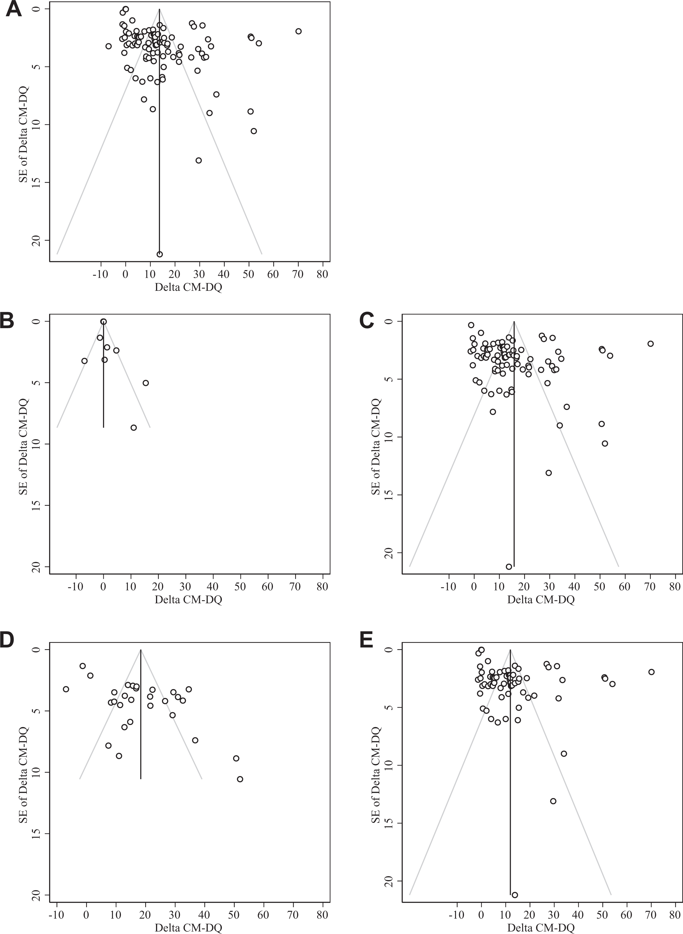
Funnel plots of crosswise model studies with 95% pseudo confidence intervals, effect size estimated by a random effects model. For ease of comparison, the scale of all plots has been fixed. Restricted sample (n_i = 104). (A) Full sample. (B) General populations. (C) WEIRD populations. (D) Probability samples. (E) Nonprobability samples.

As an additional investigation of the issue, we apply Egger’s test for small-study bias using random effects. A statistically significant Egger test indicates that the null hypothesis of no publication bias has to be rejected. The test statistic for the overall sample indicates a small study bias (Egger’s test = 4.76; z = 40.18; p $<$ .0001).¹²

It is important to note, to account for between-study variation of publication bias, Egger’s test can be extended to incorporate moderators (Sterne and Egger 2005). To investigate this issue, we also reestimated the funnel plots along with the Egger tests including these subgroups as moderators. The second row of Figure 3 displays funnel plots controlling for the population type. The left plot in the second row is for general populations, the right plot for WEIRD populations. The graph for general populations is asymmetric and indicates small effects in general population samples.¹³ Egger’s test produces a statistically significant result for publication bias (Egger’s test = 3.01; z = 17.21; p $<$ .0001). The right graph for WEIRD populations indicates stronger effects of larger studies. The Egger test result (Egger’s test = 5.08; z = 37.97; p $<$ .0001) suggests publication bias.

Funnel plots by sample type are presented at the bottom of Figure 3: The left plot is for probability samples; the right plot for nonprobability samples. The graph for probability samples is largely symmetric but has a few large and small study outliers. The Egger test for probability samples indicates publication bias (Egger’s test = 3.29; z = 3.93; p $<$ .0001). The plot for nonprobability samples is asymmetric with several outliers; we observe a large study effect. Again, Egger’s test statistic indicates publication bias (Egger’s test = 5.08; z = 36.38; p $<$ .0001).

We performed Duval and Tweedie’s trim and fill (Duval and Tweedie 2000) to estimate how many studies are required to achieve funnel plot symmetry and therefore no publication bias. The results suggest that 50 additional items would have to be included. We present the estimated funnel plot in Figure 5. The observed items are displayed as circles; the imputed items as triangles. This high number of potentially missing studies can be interpreted as clear evidence of publication bias.

Figure 5.

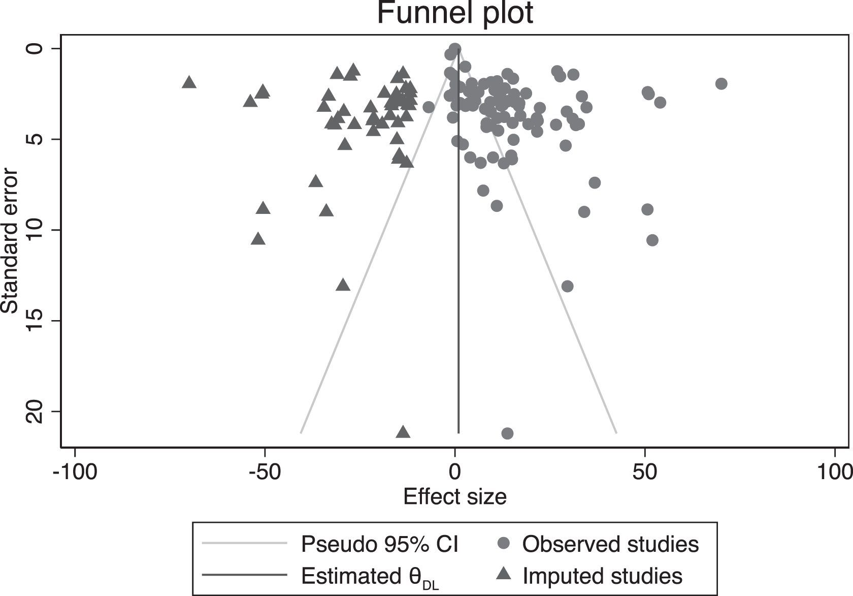
Trimmed funnel plot with 95% pseudo confidence intervals, full sample.

Meta-Regression of CM Studies With Moderators

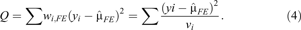
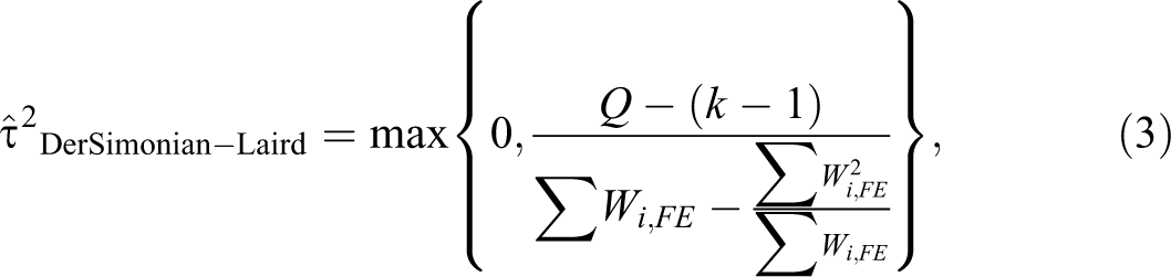
To test the impact of the population and sample type on the difference ( $Δ$ ) in the CM and DQ, random effects, meta-regression models were estimated (Raudenbush 1994:301-5).¹⁴ We use the DerSimonian–Laird estimator (DerSimonian and Laird 1986), which is one of the most frequently used estimators for random effects meta-regression (Veroniki et al. 2016). It is obtained as

{\hat{τ}}^{2}_{DerSimonian-Laird} = max \{0, \frac{Q - (k - 1)}{\sum W_{i, F E} - \frac{\sum W_{i, F E}^{2}}{\sum W_{i, F E}}}\},

where Q is calculated based on an estimate from a fixed effect (FE) analysis:

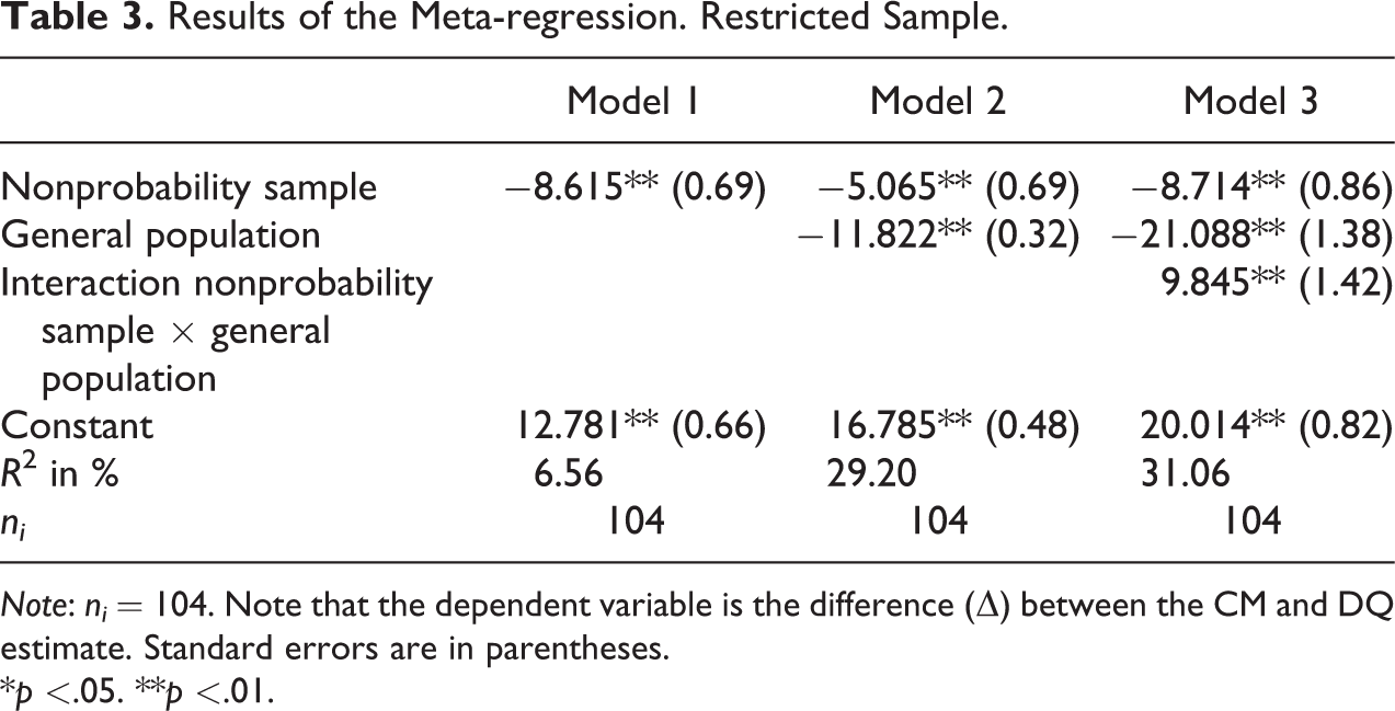
Q = \sum w_{i, F E} {(y_{i} - {\hat{μ}}_{F E})}^{2} = \sum \frac{{(y i - {\hat{μ}}_{F E})}^{2}}{v_{i}} .

The results of the meta-regression are presented in Table 3. Model 1 includes the sample type. The population type is added in model 2. Next, an interaction term between the population and sample type is included in model 3.

Table 3.

Results of the Meta-regression. Restricted Sample.

	Model 1	Model 2	Model 3
Nonprobability sample	−8.615** (0.69)	−5.065** (0.69)	−8.714** (0.86)
General population		−11.822** (0.32)	−21.088** (1.38)
Interaction nonprobability sample × general population			9.845** (1.42)
Constant	12.781** (0.66)	16.785** (0.48)	20.014** (0.82)
R ² in %	6.56	29.20	31.06
n_i	104	104	104

Note: n_i = 104. Note that the dependent variable is the difference ( $Δ$ ) between the CM and DQ estimate. Standard errors are in parentheses.

*p $<$ .05. **p $<$ .01.

The results of the meta-regression suggest that the sample and population type matter: Nonprobability samples are more likely to produce a smaller difference ( $Δ$ ) of the CM and DQ; as is also the case for general populations.

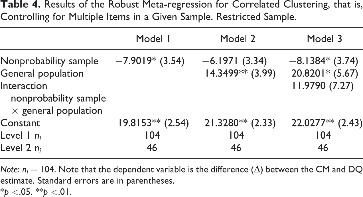
The positive interaction effect of the sample and population type suggests a larger $Δ$ of the CM and DQ when nonprobability samples and general population are concerned. However, we consider this effect as an artefact because the estimates collected in the publications on the CM are not independent. Their effects might be (1) correlated, that is, publications include multiple estimates per sample, or (2) hierarchical, that is, the same research group publishes estimates on independent samples (Stevens & Taylor 2009).

To investigate these issues, we also reestimated the models using robumeta in Stata for robust variance estimates (Hedges, Tipton, and Johnson 2010; Tanner-Smith and Tipton 2017). However, the Stata macro only allows to either estimate robust estimates for correlated or for hierarchical clustering effects. Thus, separate models controlling for each kind of clustering were estimated.

The results of the robust variance models for correlated clustering, that is, controlling for multiple items in a given sample, with $ρ$ set at 0.8 are presented in the findings in Table 4. The effects of the nonprobability samples and general populations hold with regard to the effect size and its direction, they remain statistically significant at the 5% level. The most important result is that the interaction between the sample and population type is statistically insignificant. These results based on robust estimates hold for different levels of $ρ$ , the assumed average intercorrelation across the observed effect sizes.

Table 4.

Results of the Robust Meta-regression for Correlated Clustering, that is, Controlling for Multiple Items in a Given Sample. Restricted Sample.

	Model 1	Model 2	Model 3
Nonprobability sample	−7.9019* (3.54)	−6.1971 (3.34)	−8.1384* (3.74)
General population		−14.3499** (3.99)	−20.8201* (5.67)
Interaction nonprobability sample × general population			11.9790 (7.27)
Constant	19.8153** (2.54)	21.3280** (2.33)	22.0277** (2.43)
Level 1 n_i	104	104	104
Level 2 n_i	46	46	46

Note: n_i = 104. Note that the dependent variable is the difference ( $Δ$ ) between the CM and DQ estimate. Standard errors are in parentheses.

*p $<$ .05. **p $<$ .01.

The results presented in Table 5 are for hierarchical clustering, that is, controlling for multiple studies by the same research group. The effect sizes of nonprobability samples and of general populations have a similar magnitude as in Table 3. However, only general populations reach conventional levels of statistical significance. The interaction term is statistically insignificant as in Table 4.¹⁵

Table 5.

Results of the Robust Meta-regression for Hierarchical Clustering, that is, Controlling for Multiple Studies by the Same Research Group. Restricted Sample.

	Model 1	Model 2	Model 3
Nonprobability sample	−7.0012 (7.77)	−6.8333 (4.39)	−8.1212 (4.00)
General population		−14.4618* (3.64)	−21.1348* (3.63)
Interaction no probability sample × general population			9.0569 (6.15)
Constant	19.0800 (7.03)	21.0712 (2.75)	22.0021** (0.12)
Level 1 n_i	104	104	104
Level 2 n_i	14	14	14

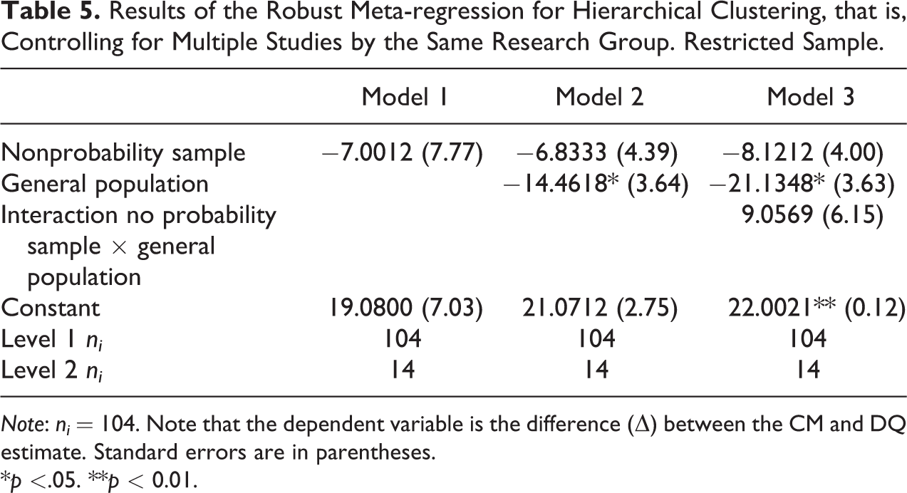
Note: n_i = 104. Note that the dependent variable is the difference ( $Δ$ ) between the CM and DQ estimate. Standard errors are in parentheses.

*p $<$ .05. **p $<$ 0.01.

Regardless of the kind of dependencies considered—correlated or hierarchical clustering—the result that general population samples are more likely to produce a smaller difference between the CM and DQ remains robust and statistically significant.

Discussion

It has been suggested that the CM is a straightforward way to estimate sensitive characteristics in survey environments, as it presumably provides more confidentiality in responses for survey respondents, who should be encouraged to more honest self-reports. To date, differences in the CM and DQ estimates capturing sensitive behavior, and thus whether or not the CM actually has a substantive gain over the DQ, has not been reviewed. This article provides a systematic review and meta-analysis studying the impact of sample and population types on whether or not the CM produces a different result than the DQ.

In sum, the results presented here raise concerns about the use of the CM in estimating sensitive characteristics. While the findings suggest heterogeneity across studies, even within the same population and sample type, the meta-regression models indicate that general populations do reduce the difference between the CM and DQ estimates. We find limited evidence that this is also the case for nonprobability samples. We consider the main result—that is, a smaller difference between the CM and DQ estimate on general population samples—to be in accordance with our hypothesis that the ability to answer questions using the CM depends on the target population. Moreover, the results suggests clear evidence of publication bias, as negative or null findings seem to be less likely to be published.

Our findings suggest that the effectiveness of the CM might be restricted to better educated subgroups, for example, students or professional survey respondents. It is desirable to test the CM and other indirect methods for estimating sensitive characteristics on probability samples of general populations. As these methods require high cognitive effort and trust, it is plausible that similar effects for related RRTs could be observed, too. Should this be case, the number of methods currently available to estimate the prevalence of sensitive characteristics in social science research diminishes sub-stantively.

Footnotes

Declaration of Conflicting Interests

The author(s) declared no potential conflicts of interest with respect to the research, authorship, and/or publication of this article.

Funding

The author(s) received no financial support for the research, authorship, and/or publication of this article.

ORCID iD

Kathrin Thomas

Notes

References

Andersen

Kasper

J. D.

Frankel

M. R.

. 1979. Total Survey Error. San Francisco, CA: Jossey-Bass.

Baker

Brick

J. M.

Bates

N. A.

Battaglia

Couper

M. P.

Denver

J. A.

Gile

K. J.

Tourangeau

. 2013. “Summary Report of the AAPOR Task Force on Nonprobability Sampling.” Journal of Survey Statistics and Methodology 1(2):90–143.

Banayejeddi

Masudi

Saeidlou

S. N.

Rezaigoyjeloo

Babaie

Abdollahi

Safaralizadeh

. 2019. “Implementation Evaluation of an Iron Supplementation Programme in High-school Students: The Crosswise Model.” Public Health Nutrition 22(14):2635–42.

Begg

C. B.

Mazumdar

1994. Operating Characteristics of a Rank Correlation Test for Publication Bias. Biometrics 50(4): 1088–1101.

Bohannon

2011. “Mechanical Turk Upends Social Sciences.” Science 352(6291):1263–64.

Bohannon

2016. “Social Science for Pennies.” Science 334(6054):307.

Borenstein

2019. “Heterogeneity in Meta-Analysis.” Pp. 453–70 in The Handbook of Research Synthesis and Meta-analysis, edited by Cooper

Hedges

L. V.

Valentine

J. C.

. New York: Russell Sage Foundation.

Borenstein

Hedges

L. V.

Higgins

J. P. T.

Rothstein

H. R.

. 2009. Introduction to Meta-analysis. Hoboken, NJ: John Wiley & Sons.

Boruch

R. F.

1971. “Assuring Confidentiality of Responses in Social Research: A Note on Strategies.” The American Sociologist 6(4):308–11.

10.

Bradburn

N. M.

Sudman

Wansink

. 2004. Asking Questions: The Definitive Guide to Questionnaire Design—For Market Research, Political Polls, and Social and Health Questionnaires. Hoboken, NJ: John Wiley & Sons.

11.

Buhrmester

M. D.

Talaifar

Gosling

S. D.

. 2011. “An Evaluation of Amazon’s Mechanical Turk. Its Rapid Rise, and Its Effective Use.” Perspectives on Psychological Science 13(2):149–54.

12.

Cannell

C. F.

Oksenberg

Converse

J. M.

. 1977. “Striving for Response Accuracy: Experiments in New Interviewing Techniques.” Journal of Marketing Research 14(3):306–15.

13.

Cannell

C. F.

Miller

P. V.

Oksenberg

. 1981. “Research on Interviewing Techniques.” Sociological Methodology 12:389–437.

14.

Chandler

Shapiro

. 2016. “Conducting Clinical Research using Crowdsourced Convenience Samples.” Annual Review of Clinical Psychology 12:53–81.

15.

Cohen

1992. “Conducting Clinical Research Using Crowdsourced Convenience Samples.” Psychological Bulletin 112(1):155–59.

16.

Corbacho

Gingerich

D. W.

Oliveros

Ruiz-Vega

. 2016. “Corruption as a Self-fulfilling Prophecy: Evidence from a Survey Experiment in Costa Rica.” American Journal of Political Science 60(4):1077–92.

17.

Cornesse

Blom

A. G.

Dutwin

Krosnick

J. A.

De Leeuw

E. D.

Legleye

Pasek

Pennay

Phillips

Sakshaug

J. W.

Struminskaya

Wenz

. 2020. “A Review of Conceptual Approaches and Empirical Evidence on Probability and Nonprobability Sample Survey Research.” Journal of Survey Statistics and Methodology 8(1):4–36.

18.

Coutts

Jann

Krumpal

Näher

A.-F.

. 2011. “Plagiarism in Student Papers: Prevalence Estimates Using Special Techniques for Sensitive Questions.” Jahrbücher für Nationalökonomie und Statistik 231(5-6):749–60.

19.

DerSimonian

Laird

. 1986. “Meta-analysis in Clinical Trials.” Controlled Clinical Trials 7(3):177–88.

20.

Duval

Tweedie

. 2000. “Trim and Fill: A Simple Funnel-plot-based Method of Testing and Adjusting for Publication Bias in Meta-analysis.” Biometrics 56(2):455–63.

21.

Egger

Smith

G. D.

Schneider

Minder

. 1997. “Bias in Meta-analysis Detected by a Simple, Graphical Test.” British Medical Journal 315(7109):629–34.

22.

Enzmann

2017. “Die Anwendbarkeit des Crosswise-Modells zur Prüfung kultureller Unterschiede sozial erwünschten Antwortverhaltens. Implikationen für seinen Einsatz in internationalen Studien zu selbstberichteter Delinquenz. [The application of the crosswise model to examine cultural differences in social desirable response behaviour. Implications for its use in international studies on self-reported delinquency.] Pp. 239–77 in Methodische Probleme von Mixed-Mode-Ansätzen in der Umfrageforschung [Methodological problems of mixed mode designs in survey research] , edited by Eifler

Faulbaum

. Wiesbaden: Springer.

23.

Enzmann

. 2020. “Email Messages to the Authors.” February 6.

24.

Enzmann

Kivivuori

Marshall

I. H.

Steketee

Hough

Killias

. 2018. “Self-reported Offending in Global Surveys: A Stocktaking.” Pp. 19–28 in A Global Perspective on Young People as Offenders and Victims. First Results from the ISRD3 Study, edited by Enzmann

Kivivuori

Marshall

I. H.

Steketee

Hough

Killias

. Cham, Switzerland: Springer.

25.

Gingerich

D. W.

Oliveros

Corbacho

Ruiz-Vega

. 2016. “When to Protect? Using the Crosswise Model to Integrate Protected and Direct Responses in Surveys of Sensitive Behavior.” Political Analysis 24(2):132–56.

26.

Greenberg

B. G.

Abul-Ela

A.-L. A.

Simmons

W. R.

Horvitz

D. G.

. 1969. “The Unrelated Question Randomized Response Model: Theoretical Framework.” Journal of the American Statistical Association 64(326):520–39.

27.

Groves

R. M.

Lyberg

. 2010. “Total Survey Error: Past, Present, and Future.” Public Opinion Quarterly 74(5):849–79.

28.

Gschwend

Juhl

Lehrer

. 2018. “Die ‘Sonntagsfrage’, soziale Erwünschtheit und die AfD: Wie alternative Messmethoden der Politikwissenschaft weiterhelfen können. [Vote intention, social desirability bias and AfD: How alternative measurement techniques can improve political research.].” Politische Vierteljahresschrift 59(3):493–519.

29.

Hedges

L. V

Tipton

Johnson

M. C.

. 2010. “Robust Variance Estimation in Meta-regression with Dependent Effect Size Estimates.” Research Synthesis Methods 1:39–65.

30.

Henrich

Heine

S. J.

Norenzayan

. 2010a. “Most People Are Not Weird.” Nature 466(7302):29.

31.

Henrich

Heine

S. J.

Norenzayan

. 2010b. “The Weirdest People in the World?” Behavioral and Brain Sciences 33(2-3):61–83.

32.

Higgins

J. P. T.

Thompson

S. G.

. 2002. “Quantifying Heterogeneity in a Meta-analysis.” Statistics in Medicine 21(11):1539–58.

33.

Hoffmann

de Puiseau

B. W.

Schmidt

A. F.

Musch

. 2017. “On the Comprehensibility and Perceived Privacy Protection of Indirect Questioning Techniques.” Behavior Research Methods 49(4):1470–83.

34.

Hoffmann

Diedenhofen

Verschuere

Musch

. 2015. “A Strong Validation of the Crosswise Model Using Experimentally-induced Cheating Behavior.” Experimental Psychology 62(6):403–14.

35.

Hoffmann

Musch

. 2019. “Prejudice against Women Leaders: Insights from an Indirect Questioning Approach.” Sex Roles 80:681–92.

36.

Hoffmann

Musch

. 2016. “Assessing the Validity of Two Indirect Questioning Techniques: A Stochastic Lie Detector versus the Crosswise Model.” Behavior Research Methods 48:1032–46.

37.

Höglinger

Diekmann

. 2017. “Uncovering a Blind Spot in Sensitive Question Research: False Positives Undermine the Crosswise-model RRT.” Political Analysis 25(1):131–37.

38.

Höglinger

Jann

. 2018. “More Is Not always Better: An Experimental Individual-level Validation of the Randomized Response Technique and the Crosswise Model.” PLoS One 13(8):1–22.

39.

Höglinger

Jann

Diekmann

. 2016. “Sensitive Questions in Online Surveys: An Experimental Evaluation of Different Implementations of the Randomized Response Technique and the Crosswise Model.” Survey Research Methods 10(3):171–87.

40.

Hopp

Speil

. 2018. “Estimating the Extent of Deceitful Behaviour Using Crosswise Elicitation Models.” Applied Economics Letters 26(5):1–5.

41.

Horvitz

D. G.

Simmons

W. R.

Shah

. 1968. “Unrelated Question Randomized Response Model.” Journal of the American Statistical Association 63(322):754–54.

42.

Jann

2005. “RRLOGIT: Stata Module to Estimate Logistic Regression for Randomized Response Data [revised 12 May 2011].” Statistical Software Components S456203, Boston College Department of Economics. Retrieved March 1, 2020 (https://ideas.repec.org/c/boc/bocode/s456203.html).

43.

Jann

Jerke

Krumpal

. 2012. “Asking Sensitive Questions using the Crosswise Model: An Experimental Survey Measuring Plagiarism.” Public Opinion Quarterly 76(1):32–49.

44.

Jerke

Johann

Rauhut

Thomas

. 2019. “Too Sophisticated Even for Highly Educated Survey Respondents? A Qualitative Assessment of Indirect Question Formats for Sensitive Questions.” Survey Research Methods 13(3):319–51.

45.

Johann

Thomas

. 2017. “Testing the Validity of the Crosswise Model: A Study on Attitudes towards Muslims.” Survey Methods: Insights from the Field. doi:10.13094/SMIF–2017–00001.

46.

Klimas

Ehlert

Lacker

T. J.

Waldvogel

Walther

. 2019. “Higher Testosterone Levels Are associated with Unfaithful Behavior in Men.” Biological Psychology 146:1–6.

47.

Korndörfer

Krumpal

Schmukle

S. C.

. 2014. “Measuring and Explaining Tax Evasion: Improving Self-reports Using the Crosswise Model.” Journal of Economic Psychology 45:18–32.

48.

Krosnick

J. A.

1991. “Response Strategies for Coping with the Cognitive Demands of Attitude Measures in Surveys.” Applied Cognitive Psychology 5(3):213–36.

49.

Krumpal

2012. “Estimating the Prevalence of Xenophobia and Anti-Semitism in Germany: A Comparison of Randomized Response and Direct Questioning.” Social Science Research 41(6):1387–1403.

50.

Krumpal

2013. “Determinants of Social Desirability Bias in Sensitive Surveys: A Literature Review.” Quality & Quantity 47(4):2025–47.

51.

Krumpal

Jann

Auspurg

von Hermanni

. 2015. “Asking Sensitive Questions: A Critical Account of the Randomized Response Technique and Related Methods.” Pp. 122–36 in Improving Survey Methods: Lessons from Recent Research, edited by Engel

Jann

Lynn

Scherpenzeel

Sturgis

. New York: Routledge.

52.

Kuk

A. Y.

1990. “Asking Sensitive Questions Indirectly.” Biometrika 77(2):436–38.

53.

Kundt

T. C.

2014. Applying Benford’s Law to the Crosswise Model: Findings from an Online Survey on Tax Evasion. Technical Report 148, Helmut-Schmidt-University, Hamburg .

54.

Kundt

T. C.

Misch

Nerré

. 2016. “Re-assessing the Merits of Measuring Tax Evasion through Business Surveys: An Application of the Crosswise Model.” International Tax and Public Finance 24(1):112–33.

55.

Lehrer

Juhl

Gschwend

. 2019. “The Wisdom of Crowds Design for Sensitive Survey Questions.” Electoral Studies 57:99–109.

56.

Lensvelt-Mulders

G. J.

Hox

J. J.

Van der Heijden

P. G.

Maas

C. J.

. 2005. “Meta-analysis of Randomized Response research: Thirty-five Years of Validation.” Sociological Methods & Research 33(3):319–48.

57.

Matthews

2008. “Probability or Nonprobability: A Survey is a Survey—or is It?” Retrieved February 24, 2020 (https://www.nass.usda.gov/Education_and_Outreach/Understanding_Statistics/Statistical_Aspects_of_Surveys/survey_is_survey.pdf).

58.

Maxfield

M. G.

Weiler

B. L.

Widom

C. S.

. 2000. “Comparing Self-reports and Official Records of Arrests.” Journal of Quantitative Criminology 16(1):87–110.

59.

Moher

Liberati

Tetzlaff

Altman

D. G.

. 2009. “Preferred Reporting Items for Systematic Reviews and Meta-Analyses: The PRISMA Statement.” PLoS Medicine 6(7). doi: 10.1371/journal.pmed.1000097.

60.

Mullinix

K. J.

Leeper

T. J.

Druckman

J. N.

Freese

. 2015. “The Generalizability of Survey Experiments.” Journal of Experimental Political Science 2(2):109–38.

61.

Nakhaee

M. R.

Pakravan

Nakhaee

. 2013. “Prevalence of Use of Anabolic Steroids by Bodybuilders Using Three Methods in a City of Iran.” Addiction & Health 5(3-4):77–81.

62.

Nasirian

Hooshyar

S. H.

Saeidifar

Taravatmanesh

Jafarnezhad

Kianersi

Haghdoost

A. A.

. 2018. “Does Crosswise Method Cause Overestimation? An Example to Estimate the Frequency of Symptoms associated with Sexually Transmitted Infections in General Population: A Cross Sectional Study.” Health Scope 7(3):1–6.

63.

Oliveros

Gingerich

D. W.

. 2019. “Lying about Corruption in Surveys: Evidence from a Joint Response Model.” International Journal of Public Opinion Research 32(2):384–95. doi: 10.1093/ijpor/edz019.

64.

Palmer

T. M.

Sterne

. 2009. Meta-analysis in Stata: An Updated Collection from the Stata Journal. Boca Raton, FL: CRC.

65.

Phillips

D. L.

Clancy

K. J.

. 1972. “Some Effects of ‘Social Desirability’ in Survey Studies.” American Journal of Sociology 77(5):921–40.

66.

Raudenbush

S. W.

1994. “Random Effect Models.” Pp. 301–21 in The Handbook of Research Synthesis and Meta-analysis, edited by Cooper

Hedges

L. V.

Valentine

J. C.

. New York: Russell Sage Foundation.

67.

Safiri

Rahimi-Movaghar

Mansournia

M. A.

Yunesian

Shamsipour

Sadeghi-Bazargani

Fotouhi

. 2018. “Sensitivity of Crosswise Model to Simplistic Selection of Nonsensitive Questions: An Application to Estimate Substance Use, Alcohol Consumption and Extramarital Sex among Iranian College Students.” Substance Use & Misuse 54(4):601–11.

68.

Schnapp

2019. “Sensitive Question Techniques and Careless Responding: Adjusting the Crosswise Model for Random Answers.” Methods, Data, Analysis 12(2):307–20.

69.

Schnell

Hill

P. B.

Esser

. 1988. Methoden empirischer Sozialforschung [Methods of empirical social research]. München, Germany: Oldenbourg.

70.

Schnell

Thomas

Noack

. 2019. “Do Respondent Education and Income Affect Survey Estimates Based on the Crosswise Model?” Working Paper, Research Methodology Group, University of Duisburg-Essen .

71.

Schwarzer

Carpenter

J. R.

Rücker

. 2015. Meta-analysis with R. Cham, Switzerland: Springer.

72.

Shamsipour

Yunesian

Fotouhi

Jann

Rahimi-Movaghar

Asghari

Akhlaghi

A. A.

. 2014. “Estimating the Prevalence of Illicit Drug Use among Students Using the Crosswise Model.” Substance Use & Misuse 49(10):1303–10.

73.

Smith

T. W.

1992. “Discrepancies between Men and Women in Reporting the Number of Sexual Partners: A Summary from Four Countries.” Social Biology 39(3-4):203–11.

74.

Sterne

J. A. C.

Egger

. 2001. “Funnel Plots for Detecting Bias in Meta-analysis: Guidelines on Choice of Axis.” Journal of Clinical Epidemiology 54(10):1046–55.

75.

Sterne

J. A. C.

Egger

. 2005. “Regression Methods to Detect Publication and Other Bias in Meta-analysis.” Pp. 99–110 in Publication Bias in Meta-analysis: Prevention, Assessment and Adjustments, edited by Rothstein

H. R.

Sutton

A. J.

Borenstein

. Hoboken, NJ: John Wiley and Sons.

76.

Sterne

J. A. C.

Egger

Smith

G. D.

. 2001. “Investigating and Dealing with Publication and other Biases.” Pp. 189–220 in Systematic Reviews in Health Care: Meta-analysis in Context, edited by Egger

Smith

G. D.

Altman

D. G.

. London: BMJ Publishing Group.

77.

Sterne

J. A. C.

Sutton

A. J.

Ioannidis

J. P. A.

Terrin

Jones

D. R.

Lau

Carpenter

Rücker

Harbord

R. M.

Schmidt

C. H.

Tezlaff

Deeks

J. J.

Peters

Macaskill

Schwarzer

Duval

Altman

D. G.

Moher

Higgins

J. P. T.

. 2011. “Recommendations for Examining and Interpreting Funnel Plot Asymmetry in Meta-analyses of Randomised Controlled Trials.” British Medical Journal 343:1–8.

78.

Stevens

J. R.

Taylor

A. M.

. 2009. “Hierarchical Dependence in Meta-analysis.” Journal of Educational and Behavioral Statistics 34(1):46–73.

79.

Tan

M. T.

Tian

G.-L.

Tang

M.-L.

. 2009. “Sample Surveys with Sensitive Questions: A Nonrandomized Response Approach.” The American Statistician 63:9–16.

80.

Tanner-Smith

E. E.

Tipton

. 2017. “Robust Variance Estimation with Dependent Effect Sizes: Practical Considerations Including a Software Tutorial in Stata and SPSS.” Research Synthesis Methods 5(1):13–30.

81.

Thomas

Johann

Kritzinger

Plescia

Zeglovits

. 2017. “Estimating Sensitive Behavior: The ICT and High-incidence Electoral Behavior.” International Journal of Public Opinion Research 29(1):157–71.

82.

Thompson

S. G.

Higgins

J. P. T.

. 2002. “How Should Meta-regression Analyses Be Undertaken and Interpreted?” Statistics in Medicine 21(11):1559–73.

83.

Tourangeau

Rips

L. J.

Rasinski

. 2000. The Psychology of Survey Response. Cambridge, MA: Cambridge University Press.

84.

Ulrich

Schröter

Striegel

Simon

. 2012. “Asking Sensitive Questions: A Statistical Power Analysis of Randomized Response Models.” Psychological Methods 17(4):623–41.

85.

Umesh

U. N.

Peterson

R. A.

. 1991. “A Critical Evaluation of the Randomized Response Method. Applications, Validation, and Research Agenda.” Sociological Methods & Research 20(1):104–138.

86.

Vakilian

Abbas Mousavi

Keramat

Chaman

. 2016. “Knowledge, Attitude, Self-efficacy and Estimation of Frequency of Condom Use among Iranian Students Based on a Crosswise Model.” International Journal of Adolescent Medicine and Health 30(1):1–5.

87.

Vakilian

Keramat

Mousavi

S. A.

Chaman

. 2019. “Experience Assessment of Tobacco Smoking, Alcohol Drinking, and Substance Use among Shahroud University Students by Crosswise Model Estimation—The Alarm to Families.” The Open Public Health Journal 12:33–37.

88.

Vakilian

Mousavi

S. A.

Keramat

. 2014. “Estimation of Sexual Behavior in the 18-to-24-Years-Old Iranian Youth Based On a Crosswise Model Study.” BMC Research Notes 7(1):1–4.

89.

Veroniki

A. A.

Jackson

Viechtbauer

Bender

Bowden

Knapp

Kuss

Higgins

J. P. T.

Langan

Salanti

. 2016. “Methods to Estimate the Between-study Variance and Its Uncertainty in Meta-analysis.” Research Synthesis Methods 7(1):55–79.

90.

Walzenbach

Hinz

. 2019. “Pouring Water into Wine: Revisiting the Advantages of the Crosswise Model for asking Sensitive Questions.” Survey Methods: Insights from the Field 1–17. doi: 10.13094/SMIF-2019-00002

91.

Warner

S. L.

1965. “Randomized Response: A Survey Technique for Eliminating Evasive Answer Bias.” Journal of the American Statistical Association 60(309):63–69.

92.

Waubert de Puiseau

Hoffmann

Musch

. 2017. “How Indirect Questioning Techniques May Promote Democracy: A Preelection Polling Experiment.” Basic and Applied Social Psychology 39(4):209–17.

93.

Weissberg

H. F.

2009. The Total Survey Error Approach: A Guide to the New Science of Survey Research. Chicago, IL: University of Chicago Press.

94.

J.-W.

Tian

G.-L.

Tang

M.-L.

. 2008. “Two New Models for Survey Sampling with Sensitive Characteristic: Design and Analysis.” Metrika 67(3):251–63.

A Meta-analysis of Studies on the Performance of the Crosswise Model

Abstract

Keywords

Introduction

Estimating Sensitive Characteristics Using the CM

Potential Effects of the CM on the Final Survey Estimates

Empirical Studies Using the CM

Systematic Review of CM Studies

Meta-Regression of CM Studies With Moderators

Discussion

Footnotes

Declaration of Conflicting Interests

Funding

ORCID iD

Notes

References